Radial Growth Patterns Associated with Tree Mortality in Nothofagus pumilio Forest


1
Instituto Argentino de Nivología, Glaciología y Ciencias Ambientales, IANIGLA-CONICET, Mendoza 5500, Argentina
2
Tree-Ring Laboratory, Lamont-Doherty Earth Observatory of Columbia University, New York, NY 10964, USA
*
Author to whom correspondence should be addressed.
Forests 2019, 10(6), 489; https://0-doi-org.brum.beds.ac.uk/10.3390/f10060489
Submission received: 25 April 2019
/
Revised: 31 May 2019
/
Accepted: 4 June 2019
/
Published: 6 June 2019
(This article belongs to the Special Issue Dieback on Drought-Prone Forest Ecosystems)
Abstract
:Tree mortality is a key process in forest dynamics. Despite decades of effort to understand this process, many uncertainties remain. South American broadleaf species are particularly under-represented in global studies on mortality and forest dynamics. We sampled monospecific broadleaf Nothofagus pumilio forests in northern Patagonia to predict tree mortality based on stem growth. Live or dead conditions in N. pumilio trees can be predicted with high accuracy using growth rate as an explanatory variable in logistic models. In Paso Córdova (CO), Argentina, where the models were calibrated, the probability of death was a strong negative function of radial growth, particularly during the six years prior to death. In addition, negative growth trends during 30 to 45 years prior to death increased the accuracy of the models. The CO site was affected by an extreme drought during the summer 1978–1979, triggering negative trends in radial growth of many trees. Individuals showing below-average and persistent negative trends in radial growth are more likely to die than those showing high growth rates and positive growth trends in recent decades, indicating the key role of droughts in inducing mortality. The models calibrated at the CO site showed high verification skill by accurately predicting tree mortality at two independent sites 76 and 141 km away. Models based on relative growth rates showed the highest and most balanced accuracy for both live and dead individuals. Thus, the death of individuals across different N. pumilio sites was largely determined by the growth rate relative to the total size of the individuals. Our findings highlight episodic severe drought as a triggering mechanism for growth decline and eventual death for N. pumilio, similar to results found previously for several other species around the globe. In the coming decades, many forests globally will be exposed to more frequent and/or severe episodes of reduced warm-season soil moisture. Tree-ring studies such as this one can aid prediction of future changes in forest productivity, mortality, and composition.
1. Introduction
In recent decades, many observations of forest decline globally have incentivized the study of the causes of forest decline and mortality related to rapidly changing climate [1,2,3,4] (and references therein). In several cases, tree mortality is preceded, from a few years to decades, by reductions in growth [5,6]. Since many factors are involved in mortality process, it remains difficult to understand why some individuals die and others stay alive within the same stand [1,3,7,8,9].
Many of the studies devoted to understanding tree mortality use annual records of stem growth preserved by tree rings [10,11,12]. Tree rings offer many advantages for the study of mortality including the accurate dating of the year of tree death, as well as the possibility of developing annual-resolved records of tree productivity without the need for periodic measurements or forest inventories [13]. In addition, dendrochronological records from around the world provide information on geographic and historical variations on forest response to climate variability at continental or hemispheric scales [14,15,16].
It is generally accepted that tree vulnerability to death is associated with previous productivity [17,18]. Negative growth trends prior to death have been observed in a large number of tree species around the world. Mortality models based on tree growth have generated consistent results for gymnosperms globally [6]. Studies on angiosperms species are less common but also appear to indicate slow growth rates previous to mortality [19,20,21]. The duration of growth decline prior to mortality varies in relation to species, site, and cause of tree death [6,21,22,23]. These decreases in long-term growth have been associated with major restrictions on hydraulic functions and/or carbon starvation [6,19,24,25,26].
Despite the above-mentioned efforts to predict tree mortality, a global understanding of how climate drives tree mortality is still lacking. This incentivizes efforts to develop and employ common methodological strategies across many sites globally to assess relationships between tree-ring-based records of growth and mortality. The representativeness of angiosperms in tree mortality studies using global databases, in particular the South American tree broadleaf species, is very poor [6,27,28,29].
Warming-induced growth reductions and forest decline are expected for the 21st century, especially in warmer and drier areas [14,30]. In Patagonian forests, growth reductions of dominant tree species since the 1980s have been related to the positive phase of the Southern Annular Mode [16,31,32]. Extreme droughts and decreasing precipitation in northern Patagonia have induced extensive forest dieback concurrent with negative trends in radial growth of Austrocedrus chilensis, Nothofagus dombeyii and Nothofagus pumilio [33,34,35,36,37]. In previous work [38], we recorded differences in tree growth trends among N. pumilio individuals with varying degrees of crown dieback in low-elevation forests. The trees with most crown dieback showed the steepest long-term negative trends in radial growth triggered by extreme drought events in the eastern-dry edge of the N. pumilio distribution [38]. The percentage of trees showing sustained declining BAI lasting two to six decades was around 44%, ranging from 22% to 88% [38]. In these forest stands, visited during the period 1998–2012, we recorded that, on average, 17% of standing trees were dead (ranging from 5% to 33%, DBH > 10 cm) [39]. Although the decrease in radial growth concurrent with the poor health of these trees suggests an increase in the probability of mortality, the growth trends of live vs. dead N. pumilio trees have not yet been compared to validate this assumption.
The objective of this study is to investigate the relationships between various tree-ring variables and the probability of mortality for N. pumilio individuals in northern Patagonia. Specifically, the objectives are to (1) determine the probability of mortality based on growth rates and trends and (2) analyze for which time intervals (short, medium, or long term) these variables best predict the N. pumilio mortality in northern Patagonian forests. We hypothesized that (1) dead trees have significantly lower growth rates and more pronounced negative growth trends than living trees under similar site conditions; and (2) models can successfully predict N. pumilio mortality at distant sites, independent from the forests in which the models were calibrated.
2. Materials and Methods
2.1. Sampling Procedures
The study sites are located in northern Patagonia, Argentina (Table 1), a mountainous region with cold wet winters and mild, relatively dry summers [40]. Three sites in pure N. pumilio stand at the eastern boundary of its distribution were selected to determine the growth patterns associated with tree mortality (Table 1). Elevations of selected plots range from 1365 to 1583 m above sea level. Due to the strong rain-shadow effect of the Andes, trees located near the eastern boundary of the N. pumilio distribution are more frequently affected by water stress than those located further west.
The probability of death was estimated based on the patterns of tree growth using logistic regression models. These models are generally used in cases where the response variable is binary (0 or 1) and the explanatory variable is continuous [41,42]. In this work, the response variable corresponds to the dead (1) or living (0) condition, while the explanatory variables correspond to growth variables as detailed below. After calibrating the models, both internal and external validations were performed.
For calibration and internal validation of the models, we used the radial growth data from trees from our most thoroughly sampled site in Paso Córdova (CO). For external validation, we used the sites Challhuaco (CH) and Perito Moreno (MO), located approximately 76 km and 141 km from CO, respectively. At CO, 60 pairs of live and dead trees from 3 adjacent plots were selected for a total of 120 trees. At CH and MO, 20 pairs of individuals were sampled, making a total of 40 pairs and 80 trees for external validation of the model (Table 1). Based on forest plots established in previous work at CO, the percentage of dead trees ranges from 21% to 33% [39].
Following the methodology proposed by Bigler and Bugman [22], we selected, within a maximum distance of 50 m between trees, pairs of dead/living trees with similar diameters and competition indexes. This paired sampling approach minimizes biases in the probability of death related to size and competition. Competition indices (CI) were calculated for each living and dead tree using the diameter at breast height for each individual tree (DBHi) and its six nearest neighboring trees (DBHj), as well as the distance between each focal tree and its six nearest neighboring trees (Distj). We calculated the Hegyi competition index [43] as follows
When one or more of the six nearest neighbors were dead, the indices were first calculated taking into account the total number of individuals and then only the living neighbors. Additional CI indices were estimated limiting the distances between the focal tree and its neighbors to a radius of 4, 5, and 6 m.
The null hypothesis of normal distribution for DBH and CI, from both living and dead trees, was tested using the Shapiro-Wilk test [44]. Since CIs for living and dead trees are not normally distributed, significant differences between them were assessed using the Kruskal-Wallis tests [45]. Given that the sample strategy was designed to avoid biases in the probability of death related to size and competition, no significant differences were expected. Considering that we could not measure the exact age of the trees due to rot in the interior of many trunks, we calculated minimum age for each individual at coring height. We also measured tree height. Differences in minimum age and height were also tested using Kruskal-Wallis tests.
2.2. Dendrochronological Analysis and Growth Variables
Two to four samples were collected from each tree at breast height using increment borers. When possible, the samples were obtained from opposite sides of the stem to avoid biases induced by eccentricity. Due to wood decay and the associated uncertainty in the dating precision, only dead trees with evidence of recent death, namely presence of bark and small branches, were selected. The dendrochronological methods described in [46] were used to date and measure the samples. The cores were mounted on wooden mounts and polished with progressively smaller grit sandpaper (from 60 to 600). Samples were visually dated and ring widths measured using a Velmex measurement system with a resolution of 0.001 mm. The dating was verified using the program COFECHA [47], which detects potential errors by comparing inter-series correlation.
To quantify changes in radial growth for both live and dead trees, we estimated the basal area increments (BAI) for each tree. The BAI is derived from the annual ring widths and the radius of each tree, being IABt = π (r2t − r2t−1), where r corresponds to the radius of the tree and t is the year of formation of the growth ring. We used the bai.out function of the dplR package [48,49] to estimate the BAIs. The bai.out function calculates BAI from the bark to the pith using the DBH of each individual and the corresponding ring-width series as inputs. In this study, the ring-width series resulted from averaging the 2–4 radii from each individual. The diameter was the DBH measured in the field.
2.3. Calibration and Validation of the Mortality Models
Logistic regression models were applied to the growth data from the CO site following the methodology proposed by Bigler and Bugmann [22]. Growth indicators (explanatory variables) were classified into two categories: “growth level” and “growth trend”. Variables considered within the “growth level” category were the means in BAI for the last 3, 5, 6, 7, 10, 15, 20, and 25 years and their respective logarithms, as well as the relative growth during the last 1, 3, 5, 6, 7, 10, 15, 20, 25, 30, 35, 40, 45, and 50 years of growth and their respective logarithms. The relative growth is the ratio between the average BAI of the selected period of growth and the total basal area (BAI/BA). The log transformation function is used to normalize the BAI distribution and reduce the disproportionate effect of very high BAI values. Variables considered within the “growth trend” category were the coefficients from linear regressions adjusted to the last 5 to 50 years of growth, every 5 years. Since some trees were 50–75 years old, we limited growth trends to the last 50 years [51].
The best logistic regression models were selected using the Akaike information criterion (AIC) [52]. Since AIC values in logistic models with small to moderate sample sizes may be biased [53,54], the Bayes information criterion (BIC) was also calculated [55]. In a first step, models with only one explanatory variable were generated and the models with the lowest AIC were selected. After that, a second explanatory variable from a different category from the first (growth level vs. growth trend) was considered [22]. The one- and two-predictor models that yielded the lowest AIC and BIC values were selected for validation.
Both internal- and cross-validation procedures were used to validate the selected models. For internal validation, we split all pairs from the CO site in half for model development, withholding the other half for model validation. This process was repeated 200 times with bootstrap resampling [22]. Predicted values >0.475 and <0.475 were assigned to "dead" and "live" conditions, respectively. Following Bigler and Bugmann [12], the threshold of 0.475 was established by dividing the number of dead individuals by the total number of alive and dead individuals, in our case 54/114. After the 200 resamplings, we calculated the average percentage of correctly classified dead and living trees for each model (i.e., successful classification rates). Notably, considering a single pre-determined threshold value (>0.475) for classification of modeled predictions of mortality can introduce bias, especially when one of the categories is over-represented. To complement the classification based on a single threshold value, we also used the value of area under the curve (AUC) [56]. The AUC is the area below the receiver operating characteristic (ROC) curve. The ROC curve relates to the sensitivity (true positive rate: Proportion of values 1, classified as 1 by the model) and the 1-specificity (false positive rate: Proportion of values 0, classified as 1 by the model) for each of the possible thresholds. The larger the area below this curve (greater AUC), the more successes a particular model has for both categories. AUC calculations were performed using R’s pROC package [56,57].
External or cross validation was carried out by applying the selected models for CO to the two independent sites: Challhuaco (CH) and Perito Moreno (MO). The threshold for classifying the predicted live-dead categories was the same as for the calibration (0.475). AUC values were also calculated for the external validation.
3. Results
3.1. DBH and Competition Index
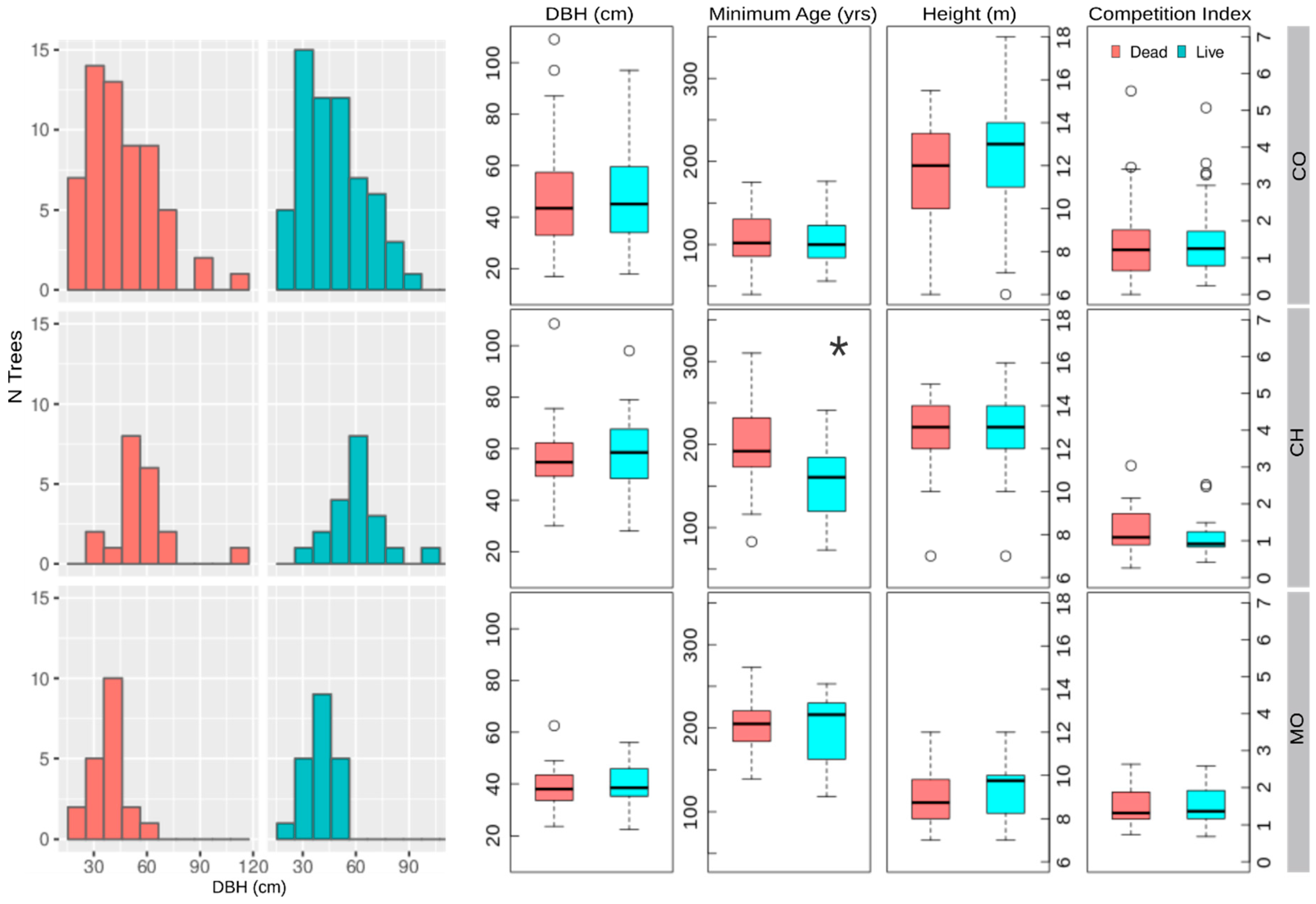
The DBH of living and dead individuals ranged from 15 to 110 cm in CO and CH, while trees in MO were between 15 and 70 cm (Figure 1). Following the sampling strategy, no significant differences in DBH and CI were found between live and dead trees at any of the three sites (Figure 1). Figure 1 also shows the results for the CIH taking into account the six nearest neighbors (including both living and standing dead trees). Similarly, no significant differences for CIH were recorded for distances of 4, 5, and 6 m between the focal tree and its neighbors, either taking into account all neighbors or only living neighbors (Results not shown). Although not significant, dead trees at CH may be more affected by competition. We did not find significant differences in terms of minimum age and height, except at the CH site where dead trees are significantly older than living trees (Figure 1).
3.2. BAI Chronologies
From a total of 120 trees sampled in CO, reliable dating was obtained from 114 trees (Table 2). The remaining trees (five dead and one alive) showed sapwood rot or low ring-width correlation with the rest of the individuals preventing the precise cross-dating. At the CH and MO sites, all individuals were successfully dated. At all sites, the mean series intercorrelation (Rbar) was high at CO and MO. Rbar at CH was lower but the expressed population signal (EPS) indicated well-replicated chronologies for all sites (Table 2) [58,59]. Cross-dated trees exhibited bark remnants, suggesting that the last ring formed in the xylem was present, providing a reliable date of tree death. According to the sampling strategy (recently dead trees), the dates of death were concentrated from year 2000 to present (Figure 2).
Differences in growth levels and trends between BAI chronologies from living and dead trees were recorded at the three sampling sites (Figure 3). Since the end of the 19th century, dead trees in CO showed a sustained increase in BAI, which stabilized at mean values around 2500 mm2/year towards the middle of the 20th century. However, these trees showed a negative trend from the 1940s onward, which became markedly pronounced during the last decades of the 20th century, reaching values of less than 1000 mm2/year or even close to 500 mm² in some years (Figure 3). On the other hand, the living trees maintained the positive trend on basal growth until the 1970s, approximately. After that, negative growth trends were also observed in living trees. However, the growth rates in living trees were higher than 1000 mm2/year for most of the 20th century and beginning of 21st century. While growth rates for both groups of trees during the early and mid-20th century were not significantly different (confidence intervals overlap), towards the end of the century, the growth rates for dead trees became significantly lower than for living trees.
Dead trees at CH had stable growth rates during the late 19th and early 20th centuries, fluctuating between 1000 and 2000 mm2/year (Figure 3). From the 1940s to present, a slightly negative trend in growth among dead trees started, becoming more pronounced in the early 1980s. Live trees showed a sustained positive trend from the end of the 19th century until present. The growth levels were significantly different between the two categories after the 1980s (no overlapping confidence intervals). The growth from live trees exceeded 2000 mm2/year after the 1950s and reached almost 3000 mm2/year in the last few decades. In contrast, the growth rates from dead trees remained mostly below 1000 mm2/year over the same period.
The chronologies from live and dead trees at MO were almost identical until the 1970s–1980s. However, after this decade, both chronologies differed markedly. While dead individuals began to show a sustained negative trend in growth, living trees followed a positive trend. At the MO site, dead and live trees maintained growth rates less than 1000 mm2/year throughout the 19th and 20th centuries except for a few years of larger growth rates during the 1920s–1930s (Figure 3). Following the 1980s, live trees had substantially higher growth rates (>1000 mm2/year) than dead trees (<100 mm2/year).
During the 19th, and through the mid-20th century, dead trees at CO and CH had greater growth rates than living trees (Figure 3). In the most recent decades, the average growth trends from dead trees were negative for the three sites, though starting in different years during the 20th century. Dead trees at CO showed the earliest and steepest negative growth trends, followed by CH and MO. Differences in growth trends were also observed among the sites for living trees. In the most recent decades, living tree growth trends were slightly negative at CO, markedly positive at CH, and relatively stable at MO (Figure 3 and Figure 4).
3.3. Logistic Models
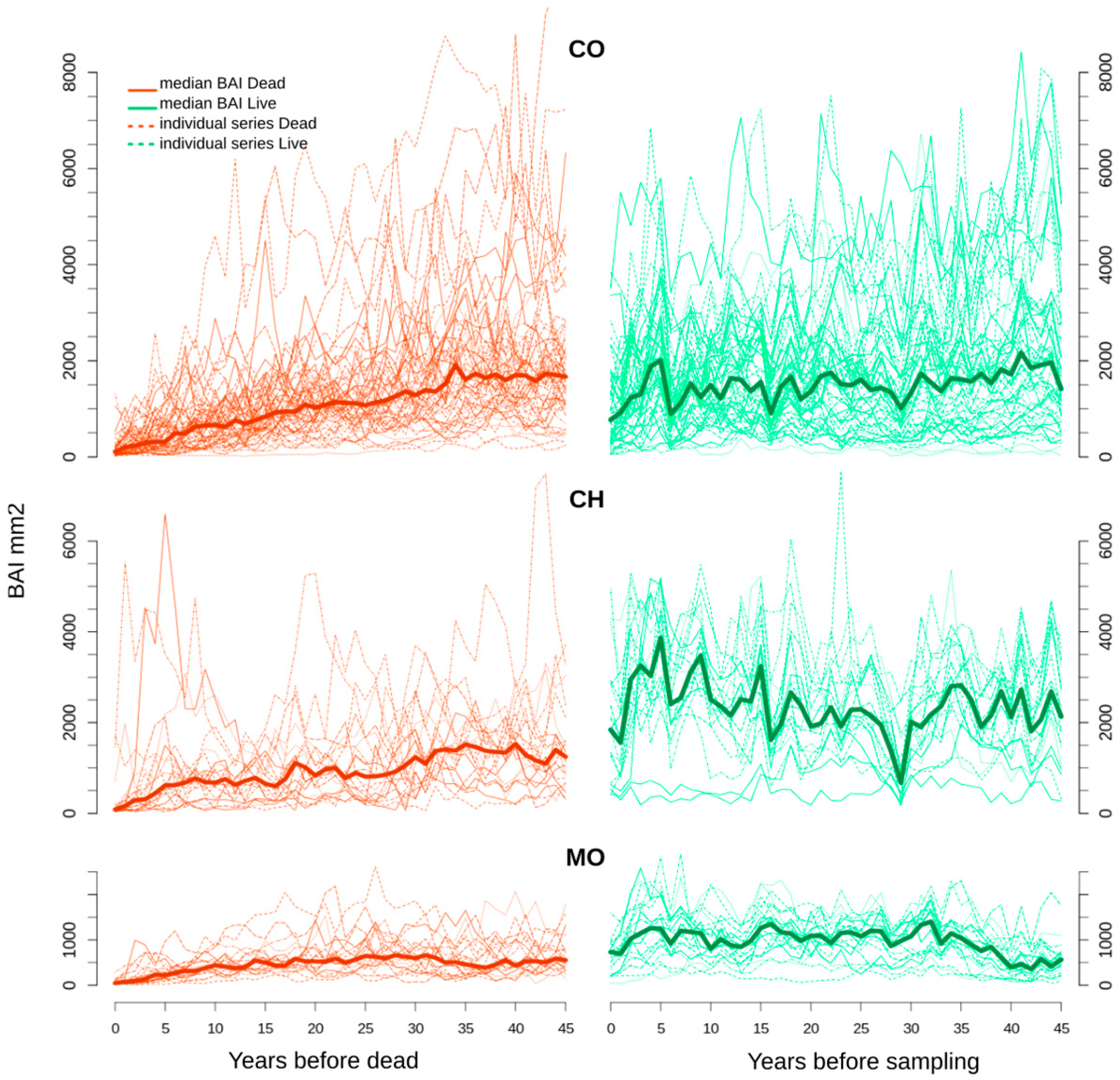
Figure 4 shows the individual and median BAI of dead (live) trees from the death year (sampling year) to the preceding 50 years. For most dead trees, a negative BAI trend starting 40 and 35 years prior to death was followed by very low BAI values over the 10 years prior to death (<1000 mm2/year), and a negative trend approaching 0 mm2/year towards the year of death. As mentioned above, trends for living trees differed between sites but all tended to decrease from five years to zero years prior to the sampling date (Figure 4). Overall, live trees showed higher growth rates than dead trees over the last 25 to 35 years. During the 50 years prior to death, some of the dead trees at CH showed growth rates similar to live trees at CO (Figure 4). Trees at MO had lower DBH than at CO and CH (Figure 1) and had lower growth rates (Figure 3). Close to the upper tree-line (1583 m asl), trees at the colder MO site were smaller than at the mesic, lower-elevation CO and CH sites. Thus, the growth rates of live MO trees did not become as high as the growth rates of live CO trees (Figure 4).
Single-predictor logistic models were calibrated for the CO site using 114 trees (59 live trees and 55 dead trees). Table 3 and Table 4 show the results for the single-predictor models with the lowest AIC and BIC values. Based on the lowest AIC and BIC values, the variables most strongly associated with likelihood of mortality were the growth level during the last 6 years (bai6, Table 3) and the growth trends of the last 40 and 35 years (locreg40 and locreg35, Table 4). In all cases, low growth rate or negative growth trend was associated with increased likelihood of mortality.
The models with two explanatory variables that had the lowest AIC and BIC values all included bai6 as the growth level predictor (Table 5), and growth trend for the last 40, 35, 30, or 45 years (locreg40, locreg35, locreg35, and locreg45). A commonly used rule in step-wise modeling is that a more complex model is superior if the AIC is reduced by >2 [60]. According to this rule, models that include bai6 and a growth trend variable for the last 40 or 35 years would be better than models based on only a single variable bai6 model. However, adding a trend variable to the bai6 model did not reduce the BIC (Table 3 and Table 5).
3.4. Validation of Logistics Models
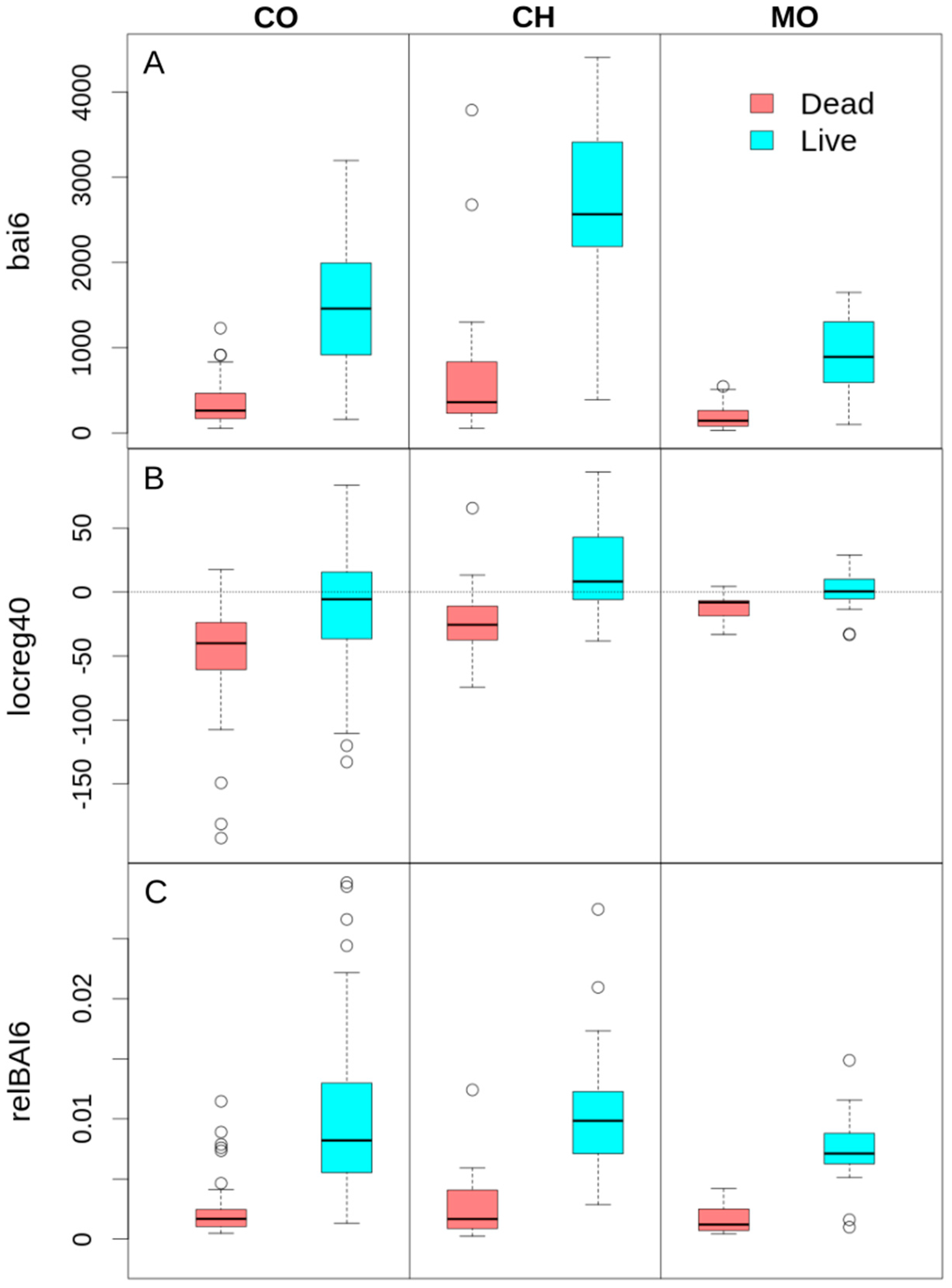
Models were generally more successful at correctly classifying the “dead” than the “live” condition of trees at CO (Table S1). This difference was less pronounced when adding growth trend as a secondary predictor to the bai6 model. Adding logreg40 to the bia6 model increased the percentage of correctly classified live trees from 81% to 85%. However, the percentage of correctly classified dead trees remained stable (93%). Several models using bai6 along with growth trends from the last 30 to 40 years as predictors showed larger percentages of internal calibration successes for live trees in CO (about 85%). Overall, both live and dead trees in CO decreased their growth during the last 40 years, but growth reductions were significantly greater for dead trees (Figure 5B).
During the external validation using 40 trees at each of the CH and MO sites, the CO-calibrated models had similarly high skill at CH and MO (Table S1). At CH, the percentage of correctly classified trees ranged between 65% and 90% for dead trees, 85% and 100% for live trees, and 77.5% and 90% for dead for all (dead and live) trees. Similarly, successful classification rates at MO varied between 80% and 100% for dead trees, 65% and 90% for live trees, and 82.5% and 95% for all trees. Contrasting results emerge for CH and MO sites regarding the predictive power of the models with the lowest AIC in the calibration stage. While the models with the lowest AIC (AIC < 77.5) correctly classified all dead individuals at MO (100%), the percentage of dead trees successfully classified at CH was closer to 70% with the same models. Conversely, 90% and 75% of live trees were correctly classified in CH and MO, respectively (Table S1).
The comprehensive analysis of the percentage of trees correctly classified by the selected models for validation reveals that the only model that equaled or exceeded the 90% of trees correctly classified in both living and dead categories at both external validation sites was the model that used relBAI6 as the sole predictor (Table S1). Only using the mean BAI during the last six years before death relative to the total BA of the tree, 90% of the dead trees were correctly classified in CO and CH, and 100% in MO. In addition, 90% of the live trees were correctly classified in MO and CH, and 78.4% in CO using the same variable. Figure 5C shows the BAI differences between live and dead trees based on the relative growth for the last six years. This model does not show the highest AIC, BIC, or AUC in the calibration stage, nor the highest number of successes in the internal validation at the CO site (Table S1).
4. Discussion
Mortality is a complex process that involves multiple causes acting simultaneously on trees from short time scales to decades [1,61]. Short-time scale disturbances can include fires, windstorms, droughts, and insect outbreaks. Here, we target mortality processes at decadal scales, likely related to the health status and growth decline of individuals and not due to short, catastrophic events that simultaneously kill many trees in a stand regardless of tree vulnerability. We analyzed the N. pumilio growth patterns from dead and live trees in northern Patagonia, Argentina, to broaden our understanding of growth characteristics predisposing trees to death or survival. From a few years to decades prior to death, trees destined to die prior to their living counterparts showed lower growth rates and steeper negative trends in radial growth than living trees. Live or dead conditions in N. pumilio individuals can be predicted with high accuracy using growth rate as an explanatory variable in logistic models. The probability of death is consistently explained by low levels of radial growth, especially during the six years prior to death. The probability of mortality is also strongly linked to negative trends in growth during the last 30 to 45 years prior to death. These results support our hypothesis and confirm that individuals showing below-average and persistent negative trends in radial growth are more likely to die than those showing high rates and positive trends in tree growth in recent decades. Our results are generally consistent with Bigler and Bugmann [22], who showed that growth rates in the last 3 years and negative trends during the last 25 years were the predictors most related to the mortality of Picea abies (L.) Karst. in the European Alps. Studies focusing on other species have also reported slower growth rates in declining or dead individuals vs. healthy individuals, serving as a potential early warning signal for tree death [19,21,62,63,64,65,66]. Particularly for the evergreen Nothofagus dombeyi in Patagonia, Suarez et al. [33] found that dead trees during the extreme drought event in 1998–1999 showed lower growth rates 30 years prior to the drought when compared with trees that survived.
Low growth rate in the several years prior to death appears to be the most important distinguishing characteristic of trees that are soon to die. At Paso Córdova (CO), the site where the models were calibrated, the mean growth during the last six years (bai6) stands out as the most powerful variable to predict the live or dead condition. Following 200 resamplings, the model with only bai6 as an explanatory variable accurately predicted 93% and 81% of dead and living trees, respectively. Although the inclusion of negative trends in growth appears less important in the models, adding the growth trends over the last 30 to 45 years increased the percentage of correctly classified living individuals. Importantly, low growth rate near the end of a tree life and a negative growth trend in the decades leading up to this time are not independent, as low growth rate is often the result of a negative growth trend [39], underscoring the importance of radial growth trends as indicators of tree vulnerability to mortality.
Rodríguez-Catón et al. [36] showed that around 1978, i.e., 37 years prior to the sampling year, a severe drought event triggered negative growth trends in N. pumilio forests with crown dieback in northern Patagonia, which has continued to the present. Both recently dead and most living trees show negative growth trends at CO since 1978, but the dead trees decreased faster than the living in the last ~40 years, reaching very low growth rates before dying (Figure 3, Figure 4 and Figure 5). 1978–1979 was also the drought year that triggered a growth decline among many Austrocedrus chilensis trees at another site in Patagonia [35]. Other studies have also shown the role of droughts in triggering negative growth trends and increasing the risk of mortality [67,68,69,70,71]. Once the negative trend begins, most individuals remained alive for several decades prior to death. Although micro-site conditions, age, and competition may influence tree vulnerability, extreme droughts and warming have also been related to growth decline and mortality in Fagaceae species such as oak [5,72,73,74]. The comparatively lower percentage of correctly classified living trees may reflect the declining condition of the forest in CO [36]. The misclassification of 15–19% of living trees in CO may be related to the negative growth trends starting in 1978 in these individuals. These results are also in accordance with those from Suarez et al. [33] who identified a match between a regional drought event in 1956–1957 and the approximate date when growth trajectories of live and dead adult trees diverged. We plan to monitor these trees over the next decade to see if model results provide a premature classification of future mortality of living but declining individuals.
While tree mortality results from the interaction of several factors such as site, species, biotic, and abiotic agents [1,61,75,76], the ultimate cause of death in the N. pumilio trees may be related to insufficient carbon production required for maintenance or repair of damaged tissues due to xylem cavitation [62]. However, additional observations related to carbohydrate production and accumulation in N. pumilio are necessary to test this hypothesis [26,77,78,79,80]. At the same time, studies on hydraulic mechanisms, wood density, and genetic differences between dead and living individuals would provide additional insights to the ultimate cause of mortality. Piper and Fajardo [81] found negative BAI trends related to age in N. pumilio but no evidence of carbon limitation related with age or height, since non-structural carbohydrates did not decline with age or height. These authors proposed that declining wood density in older and taller trees could prevent carbon limitation by increasing water storage capacity. The role of lower wood density in increasing water storage capacity and associated resistance to cavitation was also proposed for drier Nothofagus sites including N. pumilio in Patagonia [82]. Wood density, together with other hydraulic functional traits such us higher hydraulic capacitance of the leaves and stems, higher ability to recover hydraulic conductivity, and tighter stomatal control of evaporative losses, are important to survive to droughts, as shown in surviving Austrocedrus chilensis vs. dying Nothofagus dombeyi trees growing at the same site after the 1998–1999 drought in northern Patagonia [33,83]. In recent decades, particularly from 1980 onwards, increased water use efficiency and rising delta 118O in lower and upper elevation N. pumilio forests have likely resulted from drying environmental conditions [32]. However, greater plasticity in ecophysiological traits (e.g., stomatal conductance) of low elevation forest may become an advantage for these forests under a warmer climate [84,85].
Insects or pathogens may also be important in determining tree death as these biotic agents may act opportunistically on weakened trees [86,87,88]. In northern Patagonia, N. pumilio forests are exposed to insect outbreak events related to dry and warm springs [89]. In previous studies we also observed that declining trees tended to show signs of damage from bark beetles and woodpeckers, but other biotic agents present in the stem or crown such as hemiparasitic plants, fungi, and lichen did not differ between declining and healthy individuals [90]. The presence of woodpecker cavities in declining vs. healthy N. pumilio trees has also been reported in other study also relating tree dieback and growth decline to regional droughts [91], but the presence of birds may be also related to the availability of wood-boring larvae [92].
Our second hypothesis that a tree-ring-based mortality model from one site can be used to predict mortality at other sites was partially supported by our results. Despite some differences in terms of growth rates, size, and age between the three sites, the models calibrated for the CO site showed, in general, >80% of correctly classified trees (both live and dead) at the CH and MO sites (Table S1). However, differences between the percentages of accurately classified live and dead trees at both sites revealed interesting discrepancies between sites and models. The bai6 + locreg40 model had less classification skill for dead individuals at CH (70%) than at CO (93%), which may reflect the higher growth rate along with less negative growth trends among some dead trees at CH compared to CO (Figure 4 and Figure 5). In other words, some dead trees at CH have growth levels and trends similar to the live CO trees, and therefore, are classified as likely to be living. A similar situation occurs at the MO site, although there, a few live trees are erroneously classified as dead. Indeed, since the growth rates of some live trees at MO are not as high as those at CO, the models classify these few trees as dead (Figure 4 and Figure 5).
To overcome the differences related to tree size, age, or stand histories between the three sites, other predictors were analyzed. We observed a greater ability to predict the living and dead conditions for the model based on relBAI6 as a predictor, suggesting that the death of individuals across different sites is largely determined by low levels of growth relative to the total size of the individuals. In order to have low BAI relative to the total BA in the last six years, it is likely that larger values of BAI during some period before the present was followed by negative growth trends. Although the applicability of our models may be limited to mortality related to growth decline and climate variability, we correctly classified 90% or more of the trees using BAI relative to tree size at sites reserved for validation. Similar results were documented for other species and sites demonstrating the importance of growth performance relative to tree size in determining tree mortality across different biomes [93,94]. Given the regional extent of growth decline related to climate changes in the last decades of the widespread Nothofagus pumilio and other Patagonian species, our results may be relevant for future predictions of forest mortality during the 21st century.
Accurate prediction of forest responses to climate change are key for adaptive forest management. Previous studies showed evidence of long-term negative growth trends prior to death in both gymnosperms and shade-tolerant angiosperms [6]. However, evidence of long-term negative pre-death trends for drought-tolerant angiosperms is very scarce [19,20]. This lack of evidence could be related to the relatively low representation of broadleaf species in the literature [4,6,64,94,95]. Likewise, studies with South American deciduous species are comparatively scarce [33,37,38,39]. To the best of our knowledge, this paper provides the first evidence for longstanding negative trends prior to death, as well as low levels of growth six years prior to death, for a deciduous subalpine angiosperm species in the Southern Hemisphere. We followed previously used and generally accepted methodologies for predicting the living-dead condition of trees [6,12,22,51], providing new information from deciduous South American species, which now can be compared with other species from various biomes worldwide. In the coming decades, many forests will likely be exposed to more frequent episodes of reduced warm-season soil water availability and higher atmospheric moisture demand. Long records of tree-ring growth appear capable of improving our understanding of future consequences of climate change for forest productivity and survival across a range of scales, which may be useful for adaptive forest management.
Supplementary Materials
Table S1. Validation results for logistic tree mortality models, is available online at https://0-www-mdpi-com.brum.beds.ac.uk/1999-4907/10/6/489/s1.
Author Contributions
R.V., M.R.-C., and A.S. planned and designed plot setup and collected samples for the research with the help of people mention in Acknowledgments; methodology, R.V., M.R.-C.; dendrochronological processing and formal analysis, M.R.-C.; resources and funding acquisition, R.V., M.R.-C., A.S., and A.P.W.; data curation, M.R.-C.; writing—original draft preparation, M.R.-C.; writing—review and editing, M.R.-C., R.V., A.S., and A.P.W.; supervision, R.V. and A.S.
Funding
We are grateful for support from Consejo Nacional de Investigaciones Científicas y Técnicas for providing the postdoctoral fellowship (CONICET), Argentina and BNP-PARIBAS Foundation through THEMES Project. APW was supported by NSF awards 1602581 and 1743738.
Acknowledgments
We thank Alejandra Franco Corona, Damian Aperlo and Paula Mathiansen for fieldwork assistance. Administación de Parques Nacionales provided permits for fieldwork and Centro de Ski Cerro Perito Moreno provided access to Perito Moreno site. We thank the Instituto Argentino de Nivología, Glaciología y Ciencias Ambientales (IANIGLA-CONICET) and LDEO-Columbia University for providing technical facilities. Figure 3: Code to build the plots was adapted from Bunn (2008) and Edward Cook suggested adding bootstrap confidence intervals. We thank Caroline Leland for helping with R code to perform bootstrap resampling. We appreciate the useful comments of two anonymous reviewers in a former version of the manuscript.
Conflicts of Interest
The authors declare no conflict of interest.
References
- Manion, P.D. Tree Disease Concepts; Prentice Hall: Bergen County, NJ, USA, 1981. [Google Scholar]
- Ciesla, W.M.; Donaubauer, E. Decline and Dieback of Trees and Forests: A Global Overview; Food Agriculture Organization: Rome, Italy, 1994. [Google Scholar]
- Allen, C.R.D.; Breshears, D.D.; McDowell, N.G. On underestimation of global vulnerability to tree mortality and forest die-off from hotter drought in the Anthropocene. Ecosphere 2015, 6, 1–55. [Google Scholar] [CrossRef]
- Greenwood, S.; Ruiz-Benito, P.; Martinez-Vilalta, J.; Lloret, F.; Kitzberger, T.; Allen, C.D.; Jump, A.S. Tree mortality across biomes is promoted by drought intensity, lower wood density and higher specific leaf area. Ecol. Lett. 2017, 20, 539–553. [Google Scholar] [CrossRef]
- Allen, C.D.; Macalady, A.K.; Chenchouni, H.; Bachelet, D.; McDowell, N.G.; Vennetier, M.; Cobb, N. A global overview of drought and heat-induced tree mortality reveals emerging climate change risks for forests. For. Ecol. Manag. 2010, 259, 660–684. [Google Scholar] [CrossRef] [Green Version]
- Cailleret, M. A synthesis of radial growth patterns preceding tree mortality. Glob. Chang. Biol. 2017, 23, 1–50. [Google Scholar] [CrossRef] [PubMed]
- Wang, W.; Peng, C.; Kneeshaw, D.D.; Larocque, G.R.; Luo, Z. Drought-induced tree mortality: Ecological consequences, causes, and modeling. Environ. Rev. 2012, 20, 109–121. [Google Scholar] [CrossRef]
- Wong, C.M.; Daniels, L.D. Novel forest decline triggered by multiple interactions among climate, an introduced pathogen and bark beetles. Glob. Chang. Biol. 2017, 23, 1926–1941. [Google Scholar] [CrossRef] [PubMed]
- Gessler, A.; Cailleret, M.; Joseph, J.; Schonbeck, L.; Schaub, M.; Lehmann, M.; Treydte, K.; Rigling, A.; Timofeeva, G.; Saurer, M. Drought induced tree mortality—A tree-ring isotope based conceptual model to assess mechanisms and predispositions. New Phytol. 2018, 219, 485–490. [Google Scholar] [CrossRef]
- Ogle, K.; Whitham, T.G.; Cobb, N.S. Tree-ring variation in pinyon predicts likelihood of death following severe drought. Ecology 2000, 81, 3237–3243. [Google Scholar] [CrossRef]
- Wyckoff, P.H.; Clark, J.S. The relationship between growth and mortality for seven co-occurring tree species in the southern Appalachian Mountains. Ecology 2002, 90, 604–615. [Google Scholar] [CrossRef] [Green Version]
- Bigler, C.; Bugmann, H. Predicting the Time of Tree Death Using Dendrochronological Data. Ecol. Appl. 2004, 14, 902–914. [Google Scholar] [CrossRef]
- Fritts, H.C.; Swetnam, T.W. Dendroecology: A tool for evaluating variations in past and present forest environments. In Advances in Ecological Research; Academic Press: Cambridge, MA, USA, 1989; Volume 19, pp. 111–188. [Google Scholar]
- Williams, A.P.; Michaelsen, J.; Leavitt, S.W.; Still, C.J. Using tree rings to predict the response of tree growth to climate change in the continental United States during the twenty-first century. Earth Interact. 2010, 14, 1–20. [Google Scholar] [CrossRef]
- St George, S.; Ault, T.R. The imprint of climate within Northern Hemisphere trees. Quat. Sci. Rev. 2014, 89, 1–4. [Google Scholar] [CrossRef]
- Villalba, R.; Lara, A.; Masiokas, M.H.; Urrutia, R.; Luckman, B.H.; Marshall, G.J.; Lequesne, C. Unusual Southern Hemisphere tree growth patterns induced by changes in the Southern Annular Mode. Nat. Geosci. 2012, 5, 793–798. [Google Scholar] [CrossRef]
- Soto, D.P.; Donoso, P.J.; Puettmann, K.J. Mortality in relation to growth rate and soil resistance varies by species for underplanted Nothofagus seedlings in scarified shelterwoods. New For. 2014, 655–669. [Google Scholar] [CrossRef]
- Camarero, J.J.; Gazol, A.; Sangüesa-Barreda, G.; Oliva, J.; Vicente-Serrano, S.M. To die or not to die: Early warnings of tree dieback in response to a severe drought. J. Ecol. 2015, 103, 44–57. [Google Scholar] [CrossRef]
- Drobyshev, I.; Linderson, H.; Sonesson, K. Temporal mortality pattern of pedunculate oaks in southern Sweden. Dendrochronologia 2007, 24, 97–108. [Google Scholar] [CrossRef]
- Lombardi, F.; Cherubini, P.; Lasserre, B.; Tognetti, R.; Marchetti, M. Tree rings used to assess time since death of deadwood of different decay classes in beech and silver fir forests in the central Apennines (Molise, Italy). Can. J. For. Res. 2008, 38, 821–833. [Google Scholar] [CrossRef]
- Pedersen, B. The Role of Stress in the Mortality of Midwestern Oaks as Indicated by Growth prior to Death. Ecology 1998, 79, 79–93. [Google Scholar] [CrossRef]
- Bigler, C.; Bugmann, H. Growth-dependent tree mortality models based on tree rings. Can. J. For. Res. 2003, 33, 210–221. [Google Scholar] [CrossRef]
- Macalady, A.K.; Bugmann, H. Growth-Mortality Relationships in Piñon Pine (Pinus edulis) during Severe Droughts of the Past Century: Shifting Processes in Space and Time. PLoS ONE 2014, 9. [Google Scholar] [CrossRef]
- Hartmann, H.; Adams, H.; Anderegg, W.; Jansen, S.; Zeppel, M. Research frontiers in drought-induced tree mortality: Crossing scales and disciplines. New Phytol. 2015, 205, 965–969. [Google Scholar] [CrossRef] [PubMed]
- McDowell, N.G.; Beerling, D.J.; Breshears, D.D.; Fisher, R.A.; Raffa, K.F.; Stitt, M. The interdependence of mechanisms underlying climate-driven vegetation mortality. Trends Ecol. Evol. 2011, 26, 523–532. [Google Scholar] [CrossRef] [PubMed]
- Sala, A.; Piper, F.; Hoch, G. Physiological mechanisms of drought-induced tree mortality are far from being resolved. New Phytol. 2010, 186, 274–281. [Google Scholar] [CrossRef] [PubMed]
- Choat, B.; Jansen, S.; Brodribb, T.J.; Cochard, H.; Delzon, S.; Bhaskar, R.; Zanne, A.E. Global convergence in the vulnerability of forests to drought. Nature 2012, 491, 752–755. [Google Scholar] [CrossRef] [PubMed] [Green Version]
- Anderegg, W.R.L.; Klein, T.; Bartlett, M.; Sack, L.; Pellegrini, A.F.A.; Choat, B. Meta-analysis reveals that hydraulic traits explain cross-species patterns of drought-induced tree mortality across the globe. Proc. Natl. Acad. Sci. USA 2016, 113, 5024–5029. [Google Scholar] [CrossRef] [Green Version]
- Cailleret, M.; Dakos, V.; Jansen, S.; Robert, E.M.R.; Aakala, T.; Amoroso, M.M.; Antos, J.A.; Bigler, C.; Bugmann, H.; Caccianiga, M.; et al. Early-Warning Signals of Individual Tree Mortality Based on Annual Radial Growth. Front. Plant Sci. 2019, 9, 1–14. [Google Scholar] [CrossRef]
- Sánchez-Salguero, R.; Camarero, J.J.; Gutiérrez, E.; González Rouco, F.; Gazol, A.; Sangüesa-Barreda, G.; Andreu-Hayles, L.; Linares, J.C.; Seftigen, K. Assessing forest vulnerability to climate warming using a process-based model of tree growth: Bad prospects for rear-edges. Glob. Chang. Biol. 2016, 1–15. [Google Scholar] [CrossRef]
- Álvarez, C.; Veblen, T.T.; Christie, D.; González-Reyes, Á. Relationships between climate variability and radial growth of Nothofagus pumilio near altitudinal treeline in the Andes of northern Patagonia, Chile. For. Ecol. Manag. 2015, 342, 112–121. [Google Scholar] [CrossRef]
- Fajardo, A.; Gazol, A.; Mayr, C.; Camarero, J.J. Recent decadal drought reverts warming—Triggered growth enhancement in contrasting climates in the southern Andes tree line. J. Biogeogr. 2019, 1–13. [Google Scholar] [CrossRef]
- Suarez, M.L.; Ghermandi, L.; Kitzberger, T. Factors predisposing episodic drought-induced tree mortality in Nothofagus—Site, climatic sensitivity and growth trends. J. Ecol. 2004, 92, 954–966. [Google Scholar] [CrossRef]
- Mundo, I.A.; El Mujtar, V.A.; Perdomo, M.H.; Gallo, L.A.; Villalba, R.; Barrera, M.D. Austrocedrus chilensis growth decline in relation to drought events in northern Patagonia, Argentina. Trees 2010, 24, 561–570. [Google Scholar] [CrossRef]
- Amoroso, M.M.; Daniels, L.D.; Villalba, R.; Cherubini, P. Does drought incite tree decline and death in Austrocedrus chilensis forests? J. Veg. Sci. 2015, 26, 1171–1183. [Google Scholar] [CrossRef]
- Rodríguez-Catón, M.; Villalba, R.; Morales, M.; Srur, A. Influence of droughts on Nothofagus pumilio forest decline across northern Patagonia, Argentina. Ecosphere 2016, 7, 1–17. [Google Scholar] [CrossRef]
- Venegas-González, A.; Roig Juñent, F.A.; Tomazello, M.F. Recent radial growth decline in response to increased drought conditions in the northernmost Nothofagus populations from South America. For. Ecol. Manag. 2018, 409, 94–104. [Google Scholar] [CrossRef]
- Rodríguez-Catón, M. Influencia de las Variaciones Climáticas en el Decaimiento de Bosques de Nothofagus pumilio (Poepp. et Endl.) Krasser en el norte de la Patagonia Argentina. Ph.D. Thesis, Universidad Nacional de Cuyo, Mendoza, Argentina, 2014. [Google Scholar]
- Rodríguez-Catón, M.; Villalba, R.; Srur, A.M.; Luckman, B. Long-term trends in radial growth associated with Nothofagus pumilio forest decline in Patagonia: Integrating local—Into regional-scale patterns. For. Ecol. Manag. 2015, 339, 44–56. [Google Scholar] [CrossRef]
- Villalba, R.; Lara, A.; Masiokas, M.; Delgado, S.; Aravena, J.C.; Roig, F.A.; Schmelter, A.; Wolodarsky, A.; Ripalta, A. Large-scale temperature changes across the southern andes: 20th-century variations in the context of the past 400 years. Clim. Chang. 2003, 59, 177–232. [Google Scholar] [CrossRef]
- Hosmer, D.W.; Lemeshow, S. Applied Logistic Regression, 2nd ed.; John Wiley Sons, Inc.: Hoboken, NJ, USA, 2000. [Google Scholar]
- Alenius, V.; Hökkä, H.; Salminen, H.; Jutras, S. Evaluating Estimation Methods for Logistic Regression in Modeling Individual-Tree Mortality. In Modelling Forest Systems; Amaro, A., Reed, D., Soares, P., Eds.; CABI Publishing: Wallingford, UK, 2003. [Google Scholar]
- Hegyi, F. A simulation model for managing jack-pine stands. In Growth Models for Tree and Stand Simulation; Fries, J., Ed.; Royal College of Forestry: Stockholm, Sweden, 1974; pp. 74–90. [Google Scholar]
- Shapiro, S.S.; Wilk, M.B. An analysis of variance test for normality (complete samples). Biometrika 1965, 52, 591–611. [Google Scholar] [CrossRef]
- Kruskal, W.H.; Wallis, W.A. Use of Ranks in One-Criterion Variance Analysis. J. Am. Stat. Assoc. 1952, 47, 583–621. [Google Scholar] [CrossRef]
- Stokes, M.A.; Smiley, T.L. An Introduction to Tree-Ring Dating; University of Chicago Press: Chicago, IL, USA, 1968; p. 73. [Google Scholar]
- Holmes, R.L. Computer-assisted quality control in tree-ring dating and measurement. Tree Ring Bull. 1983, 43, 69–78. [Google Scholar]
- Bunn, A.G.; Korpela, M.; Biondi, F.; Merian, P.; Qeadan, F.; Zang, C.; In dplR: Dendrochronology Program Library in R. R Package version 1.5.5. Available online: http://cran.r-project.org/package=dplR (accessed on 6 June 2019).
- R Core Team. R: A Language and Environment for Statistical Computing; R Foundation for Statistical Computing: Vienna, Austria, 2018; Available online: http://www.R-project.org (accessed on 6 June 2019).
- Bunn, A.G. A dendrochronology program library in R (dplR). Dendrochronologia 2008, 26, 115–124. [Google Scholar] [CrossRef]
- Cailleret, M.; Bigler, C.; Bugmann, H.; Camarero, J.J.; Cufar, K.; Davi, H.; Mészáros, I.; Minunno, F.; Peltoniemi, M.; Robert, E.M.; et al. Towards a common methodology for developing logistic tree mortality models based on ring-width data. Ecol. Appl. 2016, 26, 1827–1841. [Google Scholar] [CrossRef] [PubMed]
- Akaike, H. A new look at the statistical model identification. In Selected Papers of Hirotugu Akaike; Springer: New York, NY, USA, 1974; pp. 215–222. [Google Scholar]
- Hurvichl, C.M.; Tsai, C. Model Selection for Extended Quasi-Likelihood Models in Small Samples. Biometrics 1995, 51, 1077–1084. [Google Scholar] [CrossRef]
- Yanagihara, H.; Sekiguchi, R.; Fujikoshi, Y. Bias correction of AIC in logistic regression models. J. Stat. Plan. Inference 2003, 115, 349–360. [Google Scholar] [CrossRef]
- Schwarz, G. Estimating the dimension of a model. Ann. Stat. 1978, 6, 461–464. [Google Scholar] [CrossRef]
- Fawcett, T. An introduction to ROC analysis. Pattern Recognit. Lett. 2006, 35, 299–309. [Google Scholar] [CrossRef]
- Robin, X.; Turck, N.; Hainard, A.; Tiberti, N.; Lisacek, F.; Sanchez, J.C.; Müller, M. pROC: An open-source package for R and S+ to analyze and compare ROC curves. BMC Bioinform. 2011, 12, 77. [Google Scholar] [CrossRef] [PubMed]
- Wigley, T.M.L.; Briffa, K.R.; Jones, P.D. On the average value of correlated time series, with applications in dendroclimatology and hydrometeorology. J. Clim. Appl. Met. 1984, 23, 201–213. [Google Scholar] [CrossRef]
- Briffa, K.R. Interpreting high-resolution proxy climate data—The example of dendroclimatology. In Analysis of Climate Variability, Applications of Statistical Techniques; von Storch, H., Navarra, A., Eds.; Springer: Berlin, Germany, 1995; pp. 77–94. [Google Scholar]
- Burnham, K.P.; Anderson, D.R. Multimodel inference: Understanding AIC and BIC in model selection. Sociol. Meth. Res. 2004, 33, 261–304. [Google Scholar] [CrossRef]
- Franklin, J.F.; Shugart, H.H.; Harmon, M.E. Tree Death as an Ecological Process. The causes, consequences, and variability of tree mortality. BioScience 1987, 37, 550–556. [Google Scholar] [CrossRef]
- Bréda, N.; Huc, R.; Granier, A.; Dreyer, E. Temperate forest trees and stands under severe drought: A review of ecophysiological responses, adaptation processes and long-term consequences. Ann. For. Sci. 2006, 63, 625–644. [Google Scholar] [CrossRef]
- Silva, D.E. Ecologie du hêtre (Fagus sylvatica L.) en marge sud-ouest de son aire de Distribution. Ph.D. Thesis, Université Henri Poincaré, Nancy, France, 2010. [Google Scholar]
- Andersson, M.; Milberg, P.; Bergman, K.O. Low pre-death growth rates of oak (Quercus robur L.)—Is oak death a long-term process induced by dry years? Ann. For. Sci. 2011, 68, 159–168. [Google Scholar] [CrossRef]
- Berdanier, A.B.; Clark, J.S. Multiyear drought-induced morbidity preceding tree death in southeastern U.S. forests. Ecol. Appl. 2016, 26, 17–23. [Google Scholar] [CrossRef]
- Sun, S.; Qiu, L.; He, C.; Li, C.; Zhang, J.; Meng, P. Drought-affected Populus simonii Carr. Show lower growth and long-term increases in intrinsic water-use efficiency prior to tree mortality. Forests 2018, 9, 564. [Google Scholar] [CrossRef]
- Bigler, C.; Bräker, O.U.; Bugmann, H.; Dobbertin, M.; Rigling, A. Drought as an Inciting Mortality Factor in Scots Pine Stands of the Valais, Switzerland. Ecosystems 2006, 9, 330–343. [Google Scholar] [CrossRef] [Green Version]
- Hereş, A.-M.; Martínez-Vilalta, J.; Claramunt López, B. Growth patterns in relation to drought-induced mortality at two Scots pine (Pinus sylvestris L.) sites in NE Iberian Peninsula. Trees 2011, 26, 621–630. [Google Scholar] [CrossRef]
- Gea-Izquierdo, G.; Viguera, B.; Cabrera, M.; Cañellas, I. Drought induced decline could portend widespread pine mortality at the xeric ecotone in managed mediterranean pine-oak woodlands. For. Ecol. Manag. 2014, 320, 70–82. [Google Scholar] [CrossRef]
- Williams, A.P.; Allen, C.D.; Macalady, A.K.; Griffin, D.; Woodhouse, C.A.; Meko, D.M.; Swetnam, T.W.; Rauscher, S.A.; Seager, R.; Grissino-Mayer, H.D.; et al. Temperature as a potent driver of regional forest drought stress and tree mortality. Nat. Clim. Chang. 2013, 3, 292–297. [Google Scholar] [CrossRef]
- Gentilesca, T.; Camarero, J.J.; Colangelo, M.; Nolè, A.; Ripullone, F. Drought-induced oak decline in the western Mediterranean region: An overview on current evidences, mechanisms and management options to improve forest resilience Tiziana. iForest Biogeosci. For. 2017, 10, 965–969. [Google Scholar] [CrossRef]
- Drobyshev, I.; Linderson, H.; Sonesson, K. Relationship between crown condition and tree diameter growth in southern Swedish oaks. Environ. Monit. Assess. 2007, 128, 61–73. [Google Scholar] [CrossRef]
- Helama, S.; Sohar, K.; Läänelaid, A.; Mäkelä, H.M.; Raisio, J. Oak decline as illustrated through plant–climate interactions near the northern edge of species range. Bot. Rev. 2016, 82, 1–23. [Google Scholar] [CrossRef]
- Romagnoli, M.; Moroni, S.; Recanatesi, F.; Salvati, R.; Scarascia Mugnozza, G. Climate factors and oak decline based on tree-ring analysis. A case study of peri-urban forest in the Mediterranean area. Urban For. Urban Green. 2018, 34, 17–28. [Google Scholar] [CrossRef]
- Pedersen, B. Modeling tree mortality in response to short-and long-term environmental stresses. Ecol. Model. 1998, 105, 347–351. [Google Scholar] [CrossRef]
- Manion, P.D. Evolution of concepts in forest pathology. Phytopathology 2003, 93, 1052–1055. [Google Scholar] [CrossRef] [PubMed]
- McDowell, N.G.; Pockman, W.T.; Allen, C.D.; Breshears, D.D.; Cobb, N.; Kolb, T.; Plaut, J.; Sperry, J.; West, A.; Williams, D.G.; et al. Mechanisms of plant survival and mortality during drought: Why do some plants survive while others succumb to drought? New Phytol. 2008, 178, 719–739. [Google Scholar] [CrossRef] [PubMed]
- McDowell, N.G.; Allen, C.D.; Marshall, L. Growth, carbon-isotope discrimination, and drought-associated mortality across a Pinus ponderosa elevational transect. Glob. Chang. Biol. 2010, 16, 399–415. [Google Scholar] [CrossRef]
- Dickman, L.T.; Mcdowell, N.G.; Sevanto, S.; Pangle, R.E.; Pockman, W.T. Carbohydrate dynamics and mortality in a piñon-juniper woodland under three future precipitation scenarios. Plant Cell Environ. 2015, 38, 729–739. [Google Scholar] [CrossRef]
- Trugman, A.T.; Detto, M.; Bartlett, M.; Anderegg, W.R.L.; Schwalm, C.; Schaffer, B.; Pacala, S.W. Tree carbon allocation explains forest drought-kill and recovery patterns. Ecol. Lett. 2018. [Google Scholar] [CrossRef]
- Piper, F.I.; Fajardo, A. No evidence of carbon limitation with tree age and height in Nothofagus pumilio under Mediterranean and temperate climate conditions. Ann. Bot. 2011, 108, 907–917. [Google Scholar] [CrossRef]
- Bucci, S.J.; Scholz, F.G.; Campanello, P.I.; Montti, L.; Jimenez-Castillo, M.; Rockwell, F.A.; Manna, L.L.; Guerra, P.; Bernal, P.L.; Troncoso, O.; et al. Hydraulic differences along the water transport system of South American Nothofagus species: Do leaves protect the stem functionality? Tree Physiol. 2012, 32, 880–893. [Google Scholar] [CrossRef]
- Scholz, F.G.; Bucci, S.J.; Goldstein, G. Strong hydraulic segmentation and leaf senescence due to dehydration may trigger die-back in Nothofagus dombeyi under severe droughts: A comparison with the co-occurring Austrocedrus chilensis. Trees 2014, 28, 1475–1487. [Google Scholar] [CrossRef]
- Premoli, A.C.; Brewer, C.A. Environmental v. genetically driven variation in ecophysiological traits of Nothofagus pumilio from contrasting elevations. Aust. J. Bot. 2007, 55, 585–591. [Google Scholar] [CrossRef]
- Mathiasen, P.; Premoli, A.C. Living on the edge: Adaptive and plastic responses of the tree Nothofagus pumilio to a long-term transplant experiment predict rear-edge upward expansion. Oecologia 2016, 181, 607–619. [Google Scholar] [CrossRef] [PubMed]
- Das, A.J.; Stephenson, N.L.; Davis, K.P. Why do trees die? Characterizing the drivers of background tree mortality. Ecology 2016, 97, 2616–2627. [Google Scholar] [CrossRef] [PubMed]
- Desprez-Loustau, M.-L.; Marçais, B.; Nageleisen, L.-M.; Piou, D.; Vannini, A. Interactive effects of drought and pathogens in forest trees. Ann. For. Sci. 2006, 63, 597–612. [Google Scholar] [CrossRef] [Green Version]
- Anderegg, W.R.L.; Hicke, J.A.; Fisher, R.A.; Allen, C.D.; Aukema, J.; Bentz, B.; Hood, S.; Lichstein, J.W.; Macalady, A.K.; McDowell, N.; et al. Tree mortality from drought, insects, and their interactions in a changing climate. New Phytol. 2015, 208, 674–683. [Google Scholar] [CrossRef] [PubMed]
- Paritsis, J.; Veblen, T.T. Dendroecological analysis of defoliator outbreaks on Nothofagus pumilio and their relation to climate variability in the Patagonian Andes. Glob. Chang. Biol. 2011, 17, 239–253. [Google Scholar] [CrossRef]
- Rodríguez-Catón, M.; Villalba, R. Indicadores del decaimiento en bosques de Nothofagus pumilio en el norte de la Patagonia, Argentina. Madera y Bosques 2018, 24, 1–32. [Google Scholar] [CrossRef]
- Ojeda, V.S.; Suarez, M.L.; Kitzberger, T. Crown dieback events as key processes creating cavity habitat for magellanic woodpeckers. Austral. Ecol. 2007, 436–445. [Google Scholar] [CrossRef]
- Chazarreta, M.L.; Ojeda, V.S.; Trejo, A. Division of labour in parental care in the Magellanic Woodpecker Campephilus magellanicus. J. Ornithol. 2010, 152, 231–242. [Google Scholar] [CrossRef]
- Hülsmann, L. Tree Mortality in Central Europe: Empirically-Based Modeling using Long-Term Datasets. Ph.D. Thesis, ETH Zurich, Zurich, Switzerland, 2016. [Google Scholar]
- Drobyshev, I.; Niklasson, M.; Linderson, H.; Sonesson, K.; Karlsson, M.; Nilsson, S.G.; Lanner, J. Lifespan and mortality of old oaks—Combining empirical and modelling approaches to support their management in Southern Sweden. Ann. For. Sci. 2008, 65, 401. [Google Scholar] [CrossRef]
- Tulik, M.; Bijak, S. Are climatic factors responsible for the process of oak decline in Poland? Dendrochronologia 2016, 38, 18–25. [Google Scholar] [CrossRef]
Figure 1.
Frequency distribution of diameter at breast height (DBH), and box and whisker plots for DBH, minimum age at sampling height, height, and CIH for dead and live trees in Paso Córdova (CO), Challhuaco (CH), and Perito Moreno (MO) sites. Significant differences according to the Kruskal-Wallis test are indicated with an asterisk.

Figure 2.
Number of tree deaths per year at the three sample sites.

Figure 3.
Basal area increments (BAI) chronologies from dead and living trees for the selected three sites (solid lines) and 99% confidence intervals (gray polygons and dotted lines). Horizontal dashed lines represent the mean BAI value for each chronology.
Figure 3.
Basal area increments (BAI) chronologies from dead and living trees for the selected three sites (solid lines) and 99% confidence intervals (gray polygons and dotted lines). Horizontal dashed lines represent the mean BAI value for each chronology.

Figure 4.
BAI chronologies from dead (orange) and living (green) trees at the three sites (solid lines). Dashed, thin lines represent the BAIs from each tree.
Figure 4.
BAI chronologies from dead (orange) and living (green) trees at the three sites (solid lines). Dashed, thin lines represent the BAIs from each tree.

Figure 5.
Comparison between growth rate and growth trend variables for dead and live trees. (A) Mean BAI for the last six years (bai6); (B) BAI trend for the last 40 years (locreg40), and (C) average BAI for the last six years relative to the total basal area (relBAI6).
Figure 5.
Comparison between growth rate and growth trend variables for dead and live trees. (A) Mean BAI for the last six years (bai6); (B) BAI trend for the last 40 years (locreg40), and (C) average BAI for the last six years relative to the total basal area (relBAI6).


Table 1.
N. pumilio study sites. Site name and code, geographical location, altitude, and number of trees sampled at each site.
Table 1.
N. pumilio study sites. Site name and code, geographical location, altitude, and number of trees sampled at each site.
| Site | Sample | Coordinates | Altitude | N Trees | |
|---|---|---|---|---|---|
| plot | Latitute S | Longitude W | Masl | Sampled | |
| Paso Córdova | CO | 40°35′32.6″ | 71°08′33.0″ | 1365 | 120 |
| Cerro Challhuaco | CH | 41°15′41.9″ | 71°16′57.4″ | 1459 | 40 |
| Perito Moreno | MO | 41°46′41.0″ | 71°35′21.0″ | 1583 | 40 |
Table 2.
Number of dated trees, number of dated series (radii), period with more than five series, average series intercorrelation (Rbar) between series, and expressed population signal (EPS).
Table 2.
Number of dated trees, number of dated series (radii), period with more than five series, average series intercorrelation (Rbar) between series, and expressed population signal (EPS).
| Site | N Trees | N Series | Period > 5 Series | Series Intercorrelation | EPS |
|---|---|---|---|---|---|
| CO | 114 | 245 | 1844–2015 | 0.331 | 0.985 |
| CH | 40 | 79 | 1758–2015 | 0.179 | 0.907 |
| MO | 40 | 93 | 1763–2015 | 0.308 | 0.966 |
Table 3.
Best models with one explanatory variable: Growth level, ranked according to Akaike information criterion (AIC) value.
Table 3.
Best models with one explanatory variable: Growth level, ranked according to Akaike information criterion (AIC) value.
| logLik | AIC | BIC | p-Value | |
|---|---|---|---|---|
| bai6 | −37.340 | 78.7 | 84.2 | 1.65 × 10⁻⁷ *** |
| bai5 | −39.309 | 82.6 | 88.1 | 1.20 × 10⁻⁷ *** |
| logbai6 | −40.886 | 85.8 | 91.2 | 9.42 × 10⁻⁹ *** |
| bai7 | −41.032 | 86.1 | 91.5 | 9.25 × 10⁻⁸ *** |
| bai3 | −41.435 | 86.9 | 92.3 | 2.90 × 10⁻⁷ *** |
| logbai5 | −43.013 | 90 | 95.5 | 6.08 × 10⁻⁹ *** |
| logrelBAI6 | −44.034 | 92.1 | 100.1 | 4.40 × 10⁻⁹ *** |
| logrelBAI5 | −45.690 | 95.4 | 100.9 | 9.08 × 10⁻⁹ *** |
| relBAI6 | −46.531 | 97.1 | 102.5 | 2.41 × 10⁻⁷ *** |
*** indicate a significance of 99.9%
Table 4.
Best models with one explanatory variable: Growth trend, ranked according to AIC value.
| logLik | AIC | BIC | p-Value | |
|---|---|---|---|---|
| locreg40 | −69.589 | 143.2 | 148.7 | 2.10 × 10⁻⁴ *** |
| locreg35 | −70.464 | 144.9 | 150.4 | 3.82 × 10⁻⁴ *** |
| locreg30 | −71.646 | 147.3 | 152.8 | 7.99 × 10⁻⁴ *** |
| locreg45 | −72.463 | 148.9 | 154.4 | 1.26 × 10⁻³ *** |
*** indicate a significance of 99.9%
Table 5.
Best models with two explanatory variables: Growth level and growth trend, ranked according to AIC value.
Table 5.
Best models with two explanatory variables: Growth level and growth trend, ranked according to AIC value.
| logLik | AIC | BIC | p-Value 1st Variable | p-Value 2nd Variable | |
|---|---|---|---|---|---|
| bai6 + locreg40 | −34.973 | 76.0 | 84.2 | 6.20 × 10⁷ *** | 0.0484 * |
| bai6 + locreg35 | −35.05 | 76.1 | 84.3 | 5.64 × 10⁷ *** | 0.0514 |
| bai6 + locreg30 | −35.414 | 76.8 | 85.0 | 5.33 × 10⁷ *** | 0.069 |
| bai6 + locreg45 | −35.739 | 77.5 | 85.7 | 4.34 × 10⁷ *** | 0.094 |
*** indicate a significance of 99.9% ; * indicates a significance of 95%
© 2019 by the authors. Licensee MDPI, Basel, Switzerland. This article is an open access article distributed under the terms and conditions of the Creative Commons Attribution (CC BY) license (http://creativecommons.org/licenses/by/4.0/).
Share and Cite
MDPI and ACS Style
Rodríguez-Catón, M.; Villalba, R.; Srur, A.; Williams, A.P. Radial Growth Patterns Associated with Tree Mortality in Nothofagus pumilio Forest. Forests 2019, 10, 489. https://0-doi-org.brum.beds.ac.uk/10.3390/f10060489
AMA Style
Rodríguez-Catón M, Villalba R, Srur A, Williams AP. Radial Growth Patterns Associated with Tree Mortality in Nothofagus pumilio Forest. Forests. 2019; 10(6):489. https://0-doi-org.brum.beds.ac.uk/10.3390/f10060489
Chicago/Turabian StyleRodríguez-Catón, Milagros, Ricardo Villalba, Ana Srur, and A. Park Williams. 2019. "Radial Growth Patterns Associated with Tree Mortality in Nothofagus pumilio Forest" Forests 10, no. 6: 489. https://0-doi-org.brum.beds.ac.uk/10.3390/f10060489
Note that from the first issue of 2016, this journal uses article numbers instead of page numbers. See further details here.