Fine-Scale Microclimate Pattern in Forest-Steppe Habitat


1
Department of Plant Physiology and Plant Ecology, Institute of Biological Sciences, Szent István University, H-2100 Gödöllő, Hungary
2
MTA-SZIE Agroecology Research Group, Szent István University, H-2100 Gödöllő, Hungary
3
Department of Ecology, Faculty of Science and Informatics, University of Szeged, 6720 Szeged, Hungary
*
Author to whom correspondence should be addressed.
Forests 2020, 11(10), 1078; https://0-doi-org.brum.beds.ac.uk/10.3390/f11101078
Submission received: 12 September 2020
/
Revised: 3 October 2020
/
Accepted: 5 October 2020
/
Published: 9 October 2020
(This article belongs to the Special Issue Spatial Heterogeneity of Forest-Steppes)
Abstract
:Microclimate and vegetation architecture are interdependent. Little information is available, however, about the fine-scale spatio-temporal relationship between the microclimate and herb layer of forest-steppe mosaics. In 2018 a three-season-long vegetation sampling and measurements of air temperature and air humidity were performed along 4 transects (44 m long each) in the herb layer with 89 dataloggers in the sandy region of Central Hungary, in a poplar grove and the surrounding open grassland. In order to improve data analysis, we introduced the use of a duration curve widely used in hydrology and proved to be useful in the processing of intensive climatic data. We analysed the effect of the direction and altitude of the solar irradiation and the edge effect on the microclimatic pattern. We also surveyed, seasonally, the spatial pattern of the exceedance rate for the vapour pressure deficit (VPD) in relation to the transect direction and to the edge of the grove. The exceedance rate for the VPD indicated considerable seasonal differences. The VPD exceedance rate indicates the stress effect for the vegetation. The moderating effect of the grove was small at 1.2 kPa VPD, but at 3.0 kPa—stronger stress—it was considerable. On the warmer side of the transects, mostly exposed at the south-eastern edge, the exceedance rate rose abruptly with distance from the edge compared to the gradual increase on the colder side. The cardinal and intercardinal directions as well as the altitude of the Sun all had influences on the moderating and shading effects of the grove. The southern edge was not always consistently the warmest. The distribution of the VPD values above the 3.0 kPa threshold varied within a seemingly homogeneous grassland, which highlights the importance of fine-scale sampling and analysis. This knowledge is valuable for assessing the dynamics and spatio-temporal patterns of abiotic factors and physiognomy in this type of ecosystem.
1. Introduction
Climate change is expected to have a major impact on long-term community dynamics worldwide. Among other things, the global temperature increase and extreme weather events have a significant impact on the structure of forest ecosystems and also on the dynamics of environmental factors in forest patches and nearby open areas [1,2,3]. Habitats with different attributes (e.g., vegetation physiognomy and plant species composition) may respond differently to the changes, depending on their sensitivity and resilience. Transition zones could be sensitive habitats, where the structures of two different vegetation types have significant effects on each other, while their strong biotic and abiotic relationships determine the dynamics of the vegetation [4]. Typical transition zones are forest fragments, which, in many cases, are human-induced [5].
Studies about fragmented habitats have mainly focused on the effects of the surrounding open areas around the forest fragments [6,7,8]. However, there are naturally fragmented vegetation types, such as forest-steppe habitats in Central Hungary. In the case of this sandy forest-steppe vegetation, the fragmented structure has a natural origin. In this habitat, natural drying processes have been observed for decades [9,10], inhibiting the growth of woody vegetation. In addition to these processes, the seeds of tree species in this habitat can only germinate in depressions with ideal topographic conditions where a sufficient amount of water can accumulate. However, these seedlings can rarely develop into even loosely closed tree groups. Thus, the succession dynamics in a sandy-forest-steppe habitat are rather slow due to the vegetation edges, where the strong abiotic differences between the grassland and the fragment prevent forest expansion and development [10]. The sandy forest-steppe is a vegetation type that is in danger of total extinction in the near future due to the aridification in the Pannonian region [11]. Thus, improving our knowledge of this type of ecosystem is important for understanding the dynamics of abiotic and biotic factors in transition zones. Therefore, it is important to examine the effect of smaller groups of trees and larger forest patches on the surrounding grassland matrix where an edge effect is observed [12,13,14].
Among the environmental factors that characterize a habitat, the microclimate strongly influences the growth and distribution of plant species [15,16,17,18]. The most important microclimatic components that are usually examined included the air temperature, air humidity, wind force, and solar radiation [4,16]. In a study by Lin and Lin [19], environmental measurements showed that solar radiation and wind velocity had significant opposite effects on air temperature in urban vegetation. The intensity of solar radiation had a positive effect, while wind velocity had a negative effect. Thus, the cooling effect of woody vegetation is highly dependent on these factors. Hence, temperature and humidity are the main variables, from which we can also obtain the vapour pressure deficit [4,20,21]. The vapour pressure of the air in the forest and in the open areas would be similar if the vapour pressure deficit and relative humidity were determined by the air temperature. The difference in the air temperature causes the differences between the relative humidity of open and canopy-covered areas [17,22,23]. The vapour pressure deficit (VPD) can be an important limiting factor in plant growth because conditions with above-threshold values can be considered stressful. Under conditions with above-threshold values, photosynthetic CO2 uptake is strongly limited due to stomatal closure to prevent water loss [5,22,24,25].
These variables are also closely related to each other and are influenced by aspects of the vegetation structure such as the height, canopy cover, species composition, etc. [1,26]. The canopy cover directly influences the below-canopy and nearby microclimate, decreasing the solar radiation energy reaching the surface during the day while retaining outgoing longwave radiation during the night [1,26,27]. In an Atlantic forest fragment, the transient nature of the edge was observed by microclimate measurements, where the air temperature at the edge was higher than in the forest interior, while the relative humidity was lower [27]. This transient nature was also reported in a Douglas-fir forest in the U.S. [13]. Therefore, the forested areas heat up less during daytime and cool down less during night-time. In the UK, in a study of a semi-natural temperate forest, the air temperature in the forest was lower than that of the grassland and decreased from the canopy to the understory on a sunny summer day. The largest difference in air temperature between these two different areas was approximately 3 °C [12]. These microclimatic differences between open and canopy-covered areas may be much larger and more relevant, depending on the geographical location and physiognomy of the vegetation studied. Thus, little information is available about the spatio-temporal relationship between the microclimate components, the vegetation structure and ecosystem functioning in fragmented vegetations, although this knowledge is important for understanding the ecological functioning of forest ecosystems.
The edge effect is the microclimatic or vegetation structural difference between the forest edge and the interior of the forest [5]. The size of the forest patch considerably influences the extent of the edge effect and the difference between the forest interior and peripheral areas such as nearby open grassland [4,14]. According to Murcia’s review [14], there are three types of edge effects on the forest fragments. The first one is the abiotic effect, in which a change in the environmental conditions will create a habitat matrix with physical conditions different from the forest (e.g., differences in structural complexity and biomass). The two factors influencing the abiotic effects include the physiognomy and orientation. The second is the direct biological effect, in which there is a change in the abundance and distribution of species in the edge area because of differences in species tolerances. This is due to the sudden changes in the physical conditions in the edges, which may increase the tree mortality caused by wind force (wind throw) or by fire. This will lead to a change in species composition. The third is the indirect biological effect: alterations in species interactions, such as competition, predation, pollination, etc.
The stages of natural succession modify the edges during the development time; therefore, fluctuations in the distribution of plant species can be observed [28,29,30]. The current vegetation pattern corresponds to the present environmental conditions. The duration of the study is a very important parameter for such research topics, and also, the scale of sampling is relevant, but fine-scale studies are very rare [31]. Most studies about forest fragments and transition zones have used large-scale resolutions with a minimum of 20–50 m intervals between the measurement points, and the vegetation sampling has usually consisted of random, non-contiguous plots. As a result, information on fine-scale vegetation patterns is lost, and significant microclimatic differences may not be detected in the transition zone [5,13,20]. The fine-scale resolution with a sensor network helps to explore small-but-significant differences within the vegetation [31].
The main goal of this article was to assess the relationship between the microclimate and the microcoenological structure of the herb layer and to describe the microclimate-modifying effect of a grove in a sandy forest-steppe habitat. In three phenological stages of the one-year-long vegetation period, we analysed the air vapour pressure deficit (VPD) and plant species composition of the herb layer in four intersecting transects with different cardinal directions through a group of trees. The air temperature and humidity were measured in the herb layer at a fine spatial and temporal scale with 89 devices during the measurement campaigns, and 350 microcoenological relevés were made per season. We hypothesized that the VPD-modifying effect of the grove would gradually decrease in all directions away from the edge. We also assumed that the spatial microclimate patterns did not differ from season to season, that only the intensity of the modifying effect changed. The response of vegetation to the microclimate pattern was quantified according to the distribution of ecological indicator values. Our third hypothesis was that the coenological and indication structure of the herb layer differed only between the grove and the open areas and they were homogeneous in the open grassland.
2. Materials and Methods
2.1. Study Area
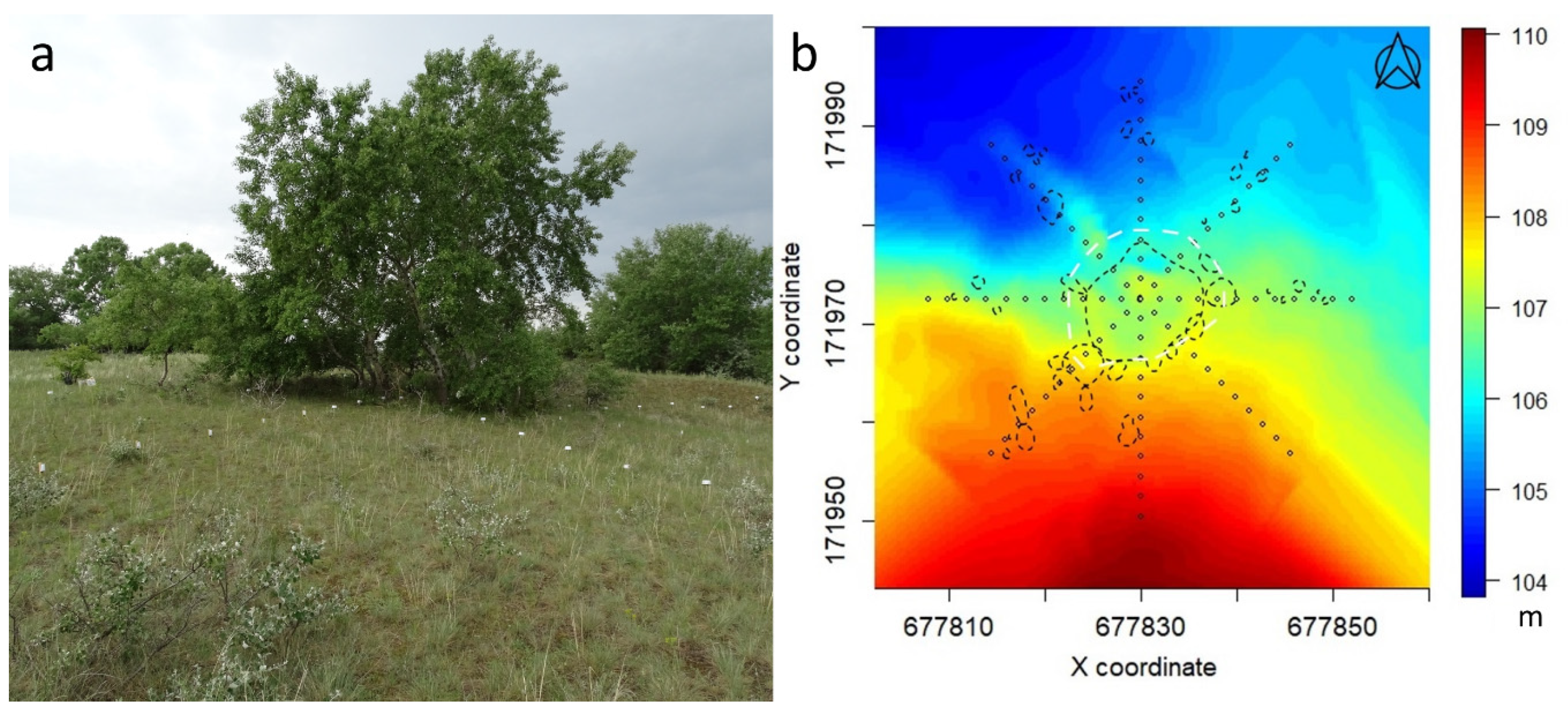
Our study site (Figure 1) was situated in Central Hungary (Fülöpháza region of the Kiskunság National Park; 46°53’28.18" N 19°24’46.91" E., 107 m a.s.l.). Throughout history, this region has been heavily cultivated, and quicksand was stopped by afforestation with invasive tree species. These processes destroyed much of the sandy forest-steppe habitat and gave space to both woody and herbaceous invasive species [10,32]. Natural forests have remained in the landscape in relatively small patches, and the sandy grasslands have, in many cases, been regenerated by secondary succession. Thus, the maintenance and restoration of the remaining natural areas is extremely important in this region. This habitat is characterized by a semi-desert climate, well indicated by the xerophytic dominant grass species, which, in the primary grasslands, are Festuca vaginata Waldst. & Kit. ex Willd. or Festuca rupicola Heuff., while the secondary grasslands contain mostly Bromus tectorum L. and Secale sylvestre Host. The dominant tree species in the natural forests are Populus alba L. or Quercus robur L., while the forest plantations are mostly dominated by Robinia pseudoacacia L. or Pinus nigra J.F. Arnold [32]. A grove of poplar (Populus alba) and the surrounding grassland were selected for this study. Measurements of microclimate components and vegetation sampling were performed in four intersecting transects (44 m long each) with different cardinal directions, forming, together, a star-shape sampling arrangement with the group of trees in the middle. The diameter of the tree group was 15 m on average.
2.2. Microclimate Measurements
Air temperature and air humidity were measured in the herb layer with a sensor network for 48 h (1-min resolution) during three measurement campaigns in different phenological stages of the vegetation in 2018 (May, July, and October). The data loggers were placed 20 cm above the soil surface, at the average height of the herbaceous vegetation, along the transects in 2 m intervals (23 measuring positions in each transect). The Crossbow MICA XM2110CA mote (Crossbow Technology Inc., Milpitas, CA, USA), UNI-T UT330B Mini USB Temperature Humidity logger (UNI-TREND Technology Co. Ltd., Guangdong, China), and Voltcraft DL-120TH USB Temperature Humidity logger (Voltcraft, Hirschau, Bavaria, Germany) were used in a sensor network, including 89 dataloggers altogether. The sensors were shielded with a white plastic plate to avoid solar radiation heating. Before the measurements, the sensors were calibrated. We selected precipitation-free measurement periods, but the sky was cloudy during the observation in May. The main changes in the weather were recorded (e.g., clouds’ shading and movement). The location of the visual edges of the grove, the positions of bushes and trees in the surrounding area, and the shadow of the grove were also recorded.
2.3. Vegetation Sampling
Vegetation data were also collected along the transects. Microcoenological relevés were recorded in 0.5 m × 0.5 m contiguous plots in each season in parallel with the micrometeorological measurements. Plant names and indicator values (TZ temperature requirement; WZ moisture requirement elaborated by Zólyomi in Table S1) were used according to FLORA Database 1.2. These ecological indicator values quantify the environmental optimums for plant species based on their occurrences in natural habitats. Lower indicator values mean lower temperature and moisture requirements, while higher values mean higher requirements [33].
2.4. Vapour Pressure Deficit and Duration Curve Method
The vapour pressure deficit was computed from the relative air humidity (RH) and air temperature (t) according to the formula developed by Bolton [21]:
with t in °C, RH in %, and VPD in Pa.
In hydrology, the “flow duration curve” is a widely used method for detecting the rate of occurrence of values for a variable above a certain critical limit (flooding degree in hydrology). With the help of this method, one can identify the duration of a flood, which means the number of days flooded during the current period [34,35]. Since micrometeorological data are large sets of fluctuating time series, similar to the hydrological data, we consider the duration curve to be a promising tool for the analysis of temperature, humidity, or vapour pressure deficit data in plant ecological studies. Our data have a diurnal cycle and may be of any temporal resolution. Our study focused primarily on the derived data, such as the percentage of the VPD values above an appropriate threshold (1.2 or 3.0 kPa) over a 24-h period (exceedance rate) that can indicate the microclimatic conditions of the vegetation. A VPD duration curve (DC) was constructed from a 24-h period of records, from 12:00 to 12:00 in each measuring position. The DC of one variable was created by sorting all the data in descending order. Thus, the rank of the highest value was 1, while that of the smallest was n (number of measurements). The ordered data can be plotted to show the DC, where the relative order (e.g., percentage) on the X-axis reflects the exceedance probability for a particular value of the variable on the Y-axis (e.g., the vapour pressure deficit at one measuring position), indicating the percentage of time a given value was equalled or exceeded over the measurement period. The tendency of the curve shows the relationship between the exceedance probabilities and the examined variable. This graph is called a period-of-record DC. Based on this method, the exceeded values can be easily determined over the measurement period [34,36].
2.5. Data Processing
Data processing was carried out on the temperature and humidity data recorded at a per-minute frequency; during 2018, altogether, more than 1,200,000 records were processed. A 24-h recording period was used to calculate the VPD and VPD exceedance rates (%) for each measurement position between 12:00 and 12:00. Statistical evaluation was performed in R [37]: VPD calculation, the spline interpolation of spatial plots (akima package) [38], principal coordinate analysis (PCoA; vegan package) [39], boxplots (calculation of average, median, min, and max), and data visualization (ggplot2 package) [40].
The principal coordinate analysis (PCoA) ordinations were made based on microcoenological data and the DCs of VPD values. In the latter case, the ordination was practically performed on the quantiles of the VPD (1% resolution). Spatial maps were generated by spline interpolation to plot the VPD data for the whole study site. The interpolation error can be smaller in this case than that when using other interpolations [41].
3. Results
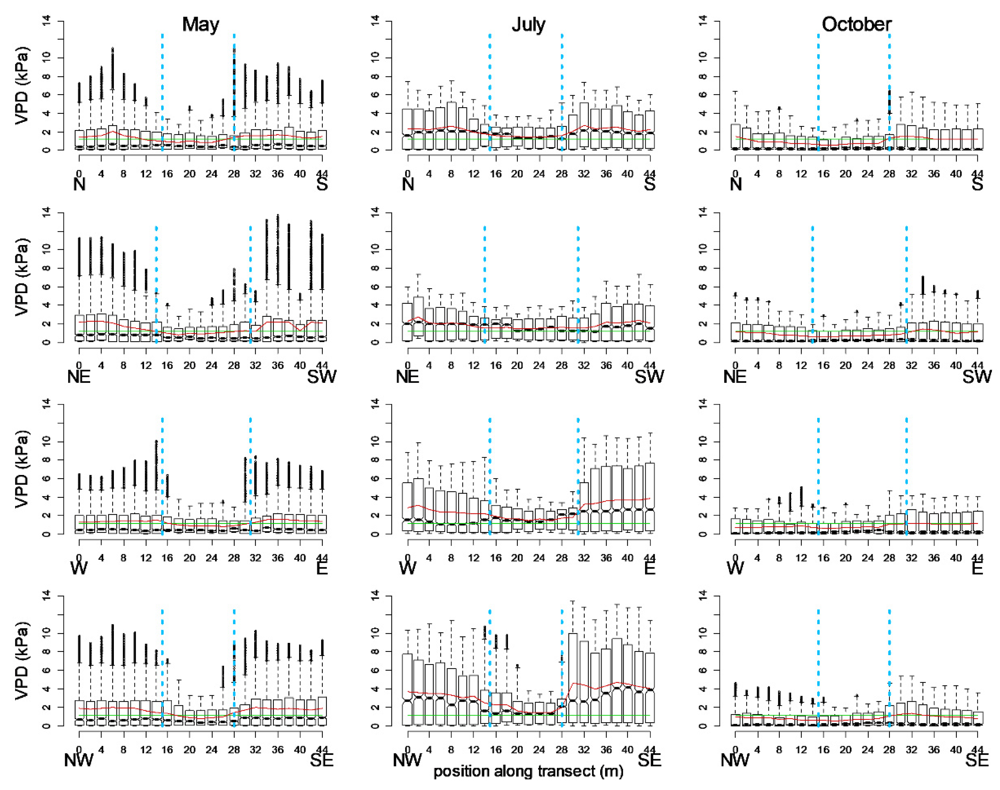
The distribution of the VPD values originating from 89 locations (4 × 22 positions in the four transects and the centre position) representing three seasons is illustrated by boxplots (Figure 2). The visually identified edges of the grove are also marked in the figures to identify the below-canopy area, the edges, and the open areas. In the figures, the left sides represent the colder sides and the right sides, the warmer ones, as determined by the irradiation and shadow patterns (cardinal directions).
During a 24-h period, differences between the grassland, edge, and below-canopy areas can be determined based on the vapour pressure deficit. The below-canopy VPD values were consistently lower than the edge or grassland VPD values. Except for the summer measurements, the below-canopy local average VPD values were lower than the threshold. The differences between the local averages and the threshold were considerable in the grassland, mostly in July. The medians of the values were very low in May and October, whereas in July, the median was mostly above the threshold. In July, the median and mean values of the below-canopy positions were very similar to each other and to the threshold. These three derivatives did not differ considerably from one another during the summer measurements (Figure 2).
The pattern of micrometeorological parameters was determined by the exposure and the position (distance) to the grove in each season. As with temperature fluctuations, the range of VPD was significantly smaller within the grove than in the open area. In the edges, we observed a special behaviour of the VPD: in the warmer edge, which was more exposed to irradiation, the values were higher with a more abrupt rise than in the open area. On the colder side of the transects, this elevated VPD did not occur at the edges, and the deficit increased more smoothly with distance from the tree group.
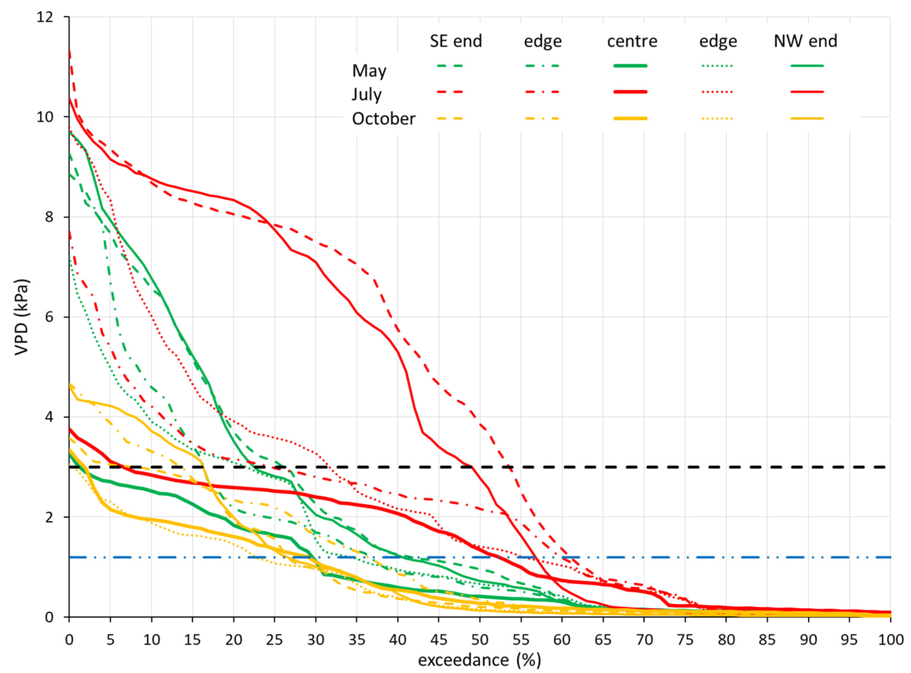
The durations of the values being over the thresholds provide important information about the spatio-temporal pattern of the VPD. Figure 3 compares the DCs of the two ends, the edges, and the centre of the SE–NW (Southeast–Northwest) transect for the three measurement periods. Among the four transects, the difference in the effect of the exposure was the most pronounced in this one, but the behaviour of the other three transects was similar. In terms of the stress threshold (1.2 kPa) exceedance rates, the summer patterns differed significantly from the spring and autumn. The exceedance rates ranged from 29% to 41% in May, from 52% to 60% in July, and from 22% to 36% in October. In terms of VPD distribution, however, further groupings emerged. The distributions of the values measured in the middle of the grove showed relatively small seasonal differences, with longer but not stronger exceedance rates measured during the summer. The exceedance rates were 29% in May, 52% in July, and 29% in October. Although the exceedance rate for 1.2 kPa showed a small variation in each measurement period, the intensity of the exceedance already differed significantly between the individual measurement positions. The duration curves of both the end-of-transect and edge measurement series ran close to each other in each period, but their distributions differed significantly. The maxima of the end-of-transect and edge series for the spring and summer measurements were in the range of 8–11 kPa, and the others were in the range of 3–5 kPa. The spring and summer measurement series ran close together, except for the summer end-of-transect (open grassland) measurement series (Figure 3). The VPDs of the latter two series of measurements, on the other hand, were well above the others, with a more-than-45% exceedance rate with respect to 3.0 kPa, while the rates for the others were below 25%. Above 2.5 kPa, the variability of the exceedance rates began to increase in all transects; therefore, we examined the exceedance at 3.0 kPa as well (Figure 3 and Figure 4b). The exceedance rates with respect to 3.0 kPa ranged from 1% to 25% in May, from 6% to 53% in July, and from 1% to 16% in October.
The exceedance rate of the autumn values with respect to the stress threshold did not differ significantly from that of the spring values of cloudy weather, but despite the sunny and warm daytime weather, the distributions above the critical limit were completely different. The maximum values did not exceed 5 kPa, and they were only slightly higher than the values below canopy.
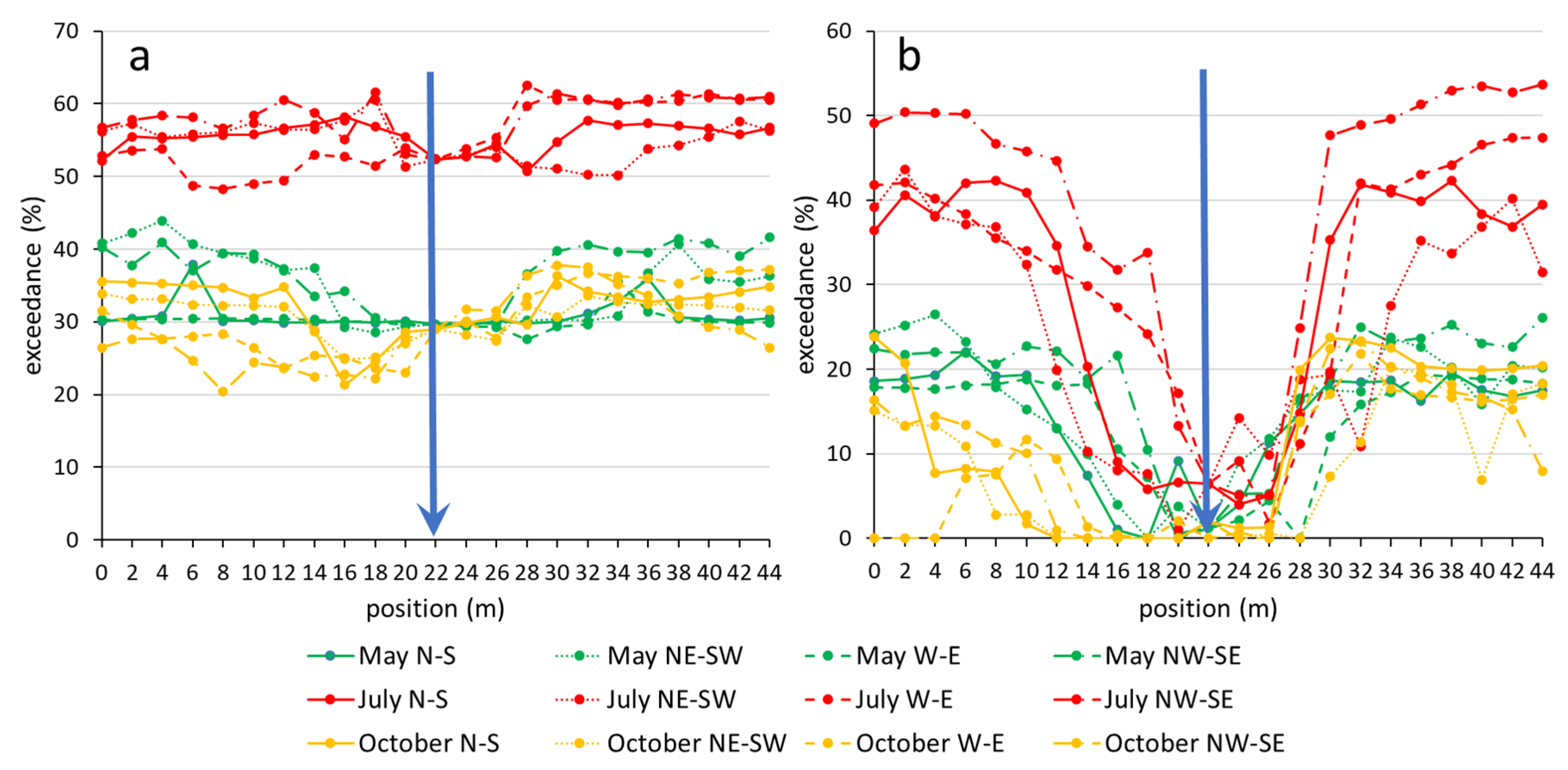
The exceedance rate with respect to the threshold of 1.2 kPa calculated from the VPD DCs also showed seasonal variability (Figure 4a). In each of the three measurement periods, at least 20% of the values were above the threshold. In the spring and autumn measurements, the exceedance rate was 20–45%, while in the summer period, it was 48–62%. Spring and autumn did not differ significantly from each other. The below-canopy exceedance rate was balanced and tended to be low, but the exceedance rate varied more across open areas. We also found differences in the VPD exceedance rate between the opposite ends of the transects. Choosing 3.0 kPa as the threshold value for the exceedance rate, the curves show a stronger difference between the areas in the opposite edges of the grove (Figure 4b). On sunny days, on the colder side, the lower values were even more pronounced when the Sun was at a lower altitude (October) at noon, with, sometimes, a 0–10% duration of values being above 3.0 kPa, as opposed to a 25–30% duration on the warmer side (Figure 5).
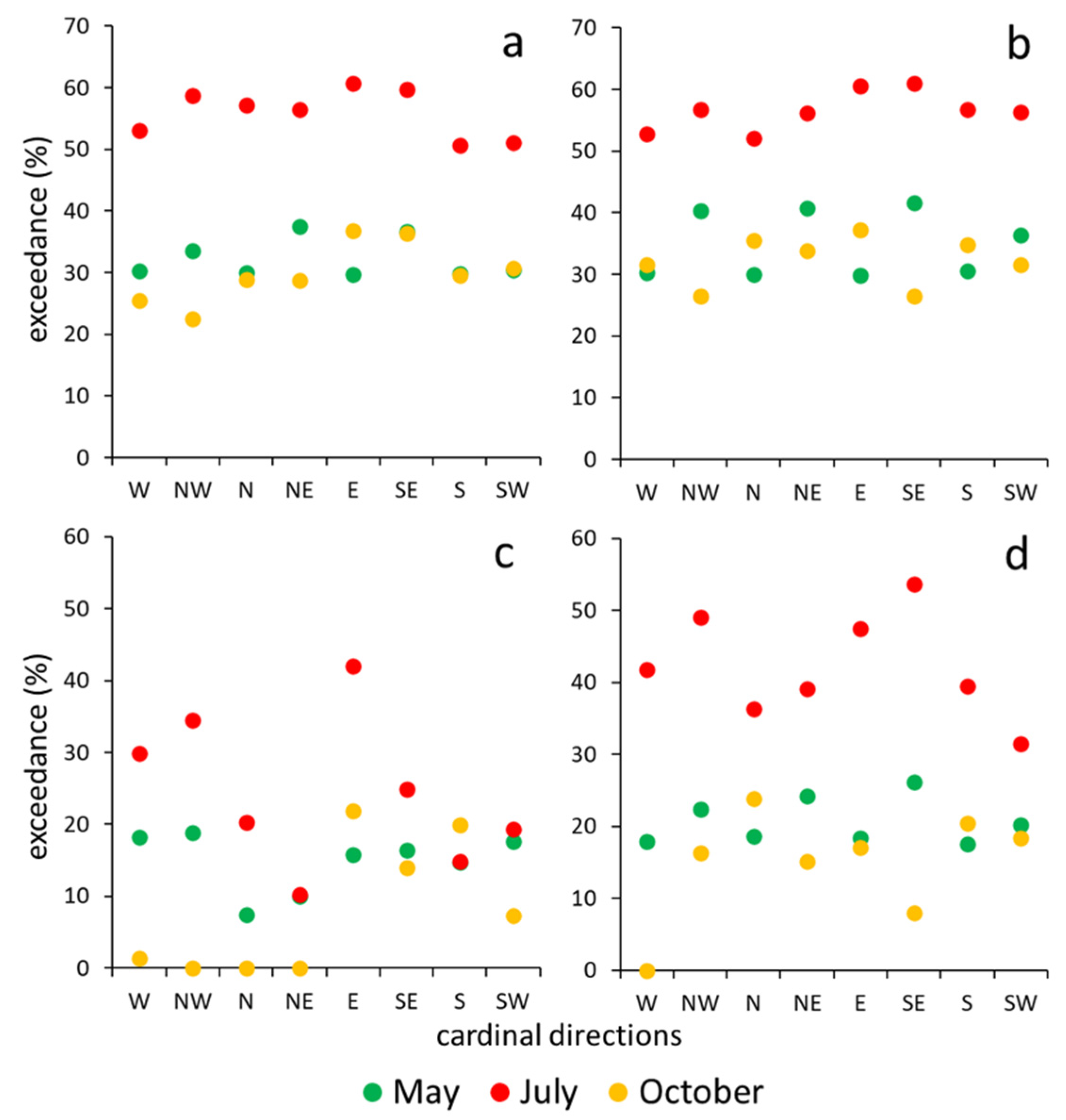
There were no remarkable differences among (all of) the edges during the spring measurements. In the case of the exceedance rate for the VPD values with respect to 1.2 kPa (Figure 5a,b), in the edges, the highest values always occurred on the eastern and south-eastern side, as well as in the grassland end positions, except for in October. In the edges, an increasing tendency could be observed from west to south-east, followed by a remarkable decreasing trend from south to west, although these trends did not appear in the case of grassland end positions. The values in the grassland varied during the three measurement periods. However, in the case of the exceedance rate of the VPD values with respect to 3.0 kPa (Figure 5c,d), the tendency was quite different in the edges. In the NW (Northwest), N (North), and NE (Northeast) edges, the exceedance rate was 0% with respect to 3.0 kPa. This tendency was also observed in May and July, but the fall was not as strong as in the October data.
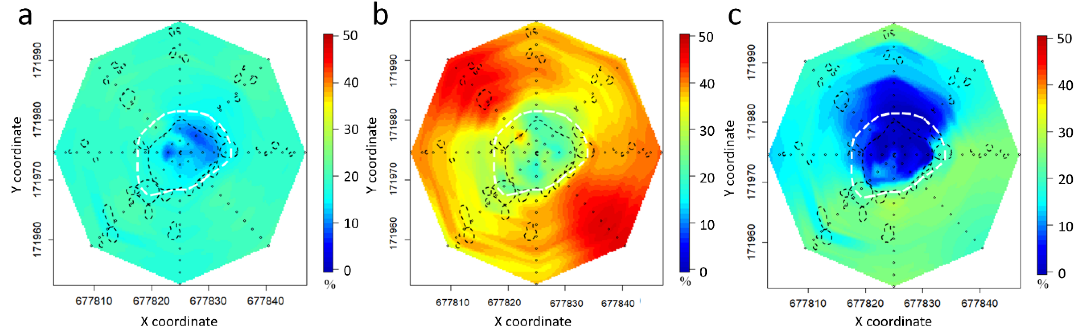
Depending on the weather conditions, the spatial pattern of the exceedance rate (Figure 6) also varied. At the 3.0 kPa threshold, the microclimatic differences among the three seasons were striking; the high VPD displayed the areas with consistently highly stressful conditions. In each of the three measurement periods, the below-canopy positions had lower values, but the values of the edges and the surrounding grassland were varied. There was only a slight difference between the open areas on the different sides of the tree group (Figure 6a). In October (Figure 6c), the transition between the warmer (E–SE (East–Southeast)) and colder (W–NW (west– Northwest)) sides was more gradual than in July (Figure 6b). In both of the later cases (summer and autumn), the measurements were made under clear skies. In July, the opposite grassland sides of the grove were in sync, NE and SW had lower values, and SE and NW had higher values. On the other hand, in October, the warmer and colder zones expanded considerably, and the transition between the two zones was sharp. In October, the warmer grassland side was E–SW, and W–NE was notably colder. In both periods, the eastern and south-eastern open areas had the highest values.
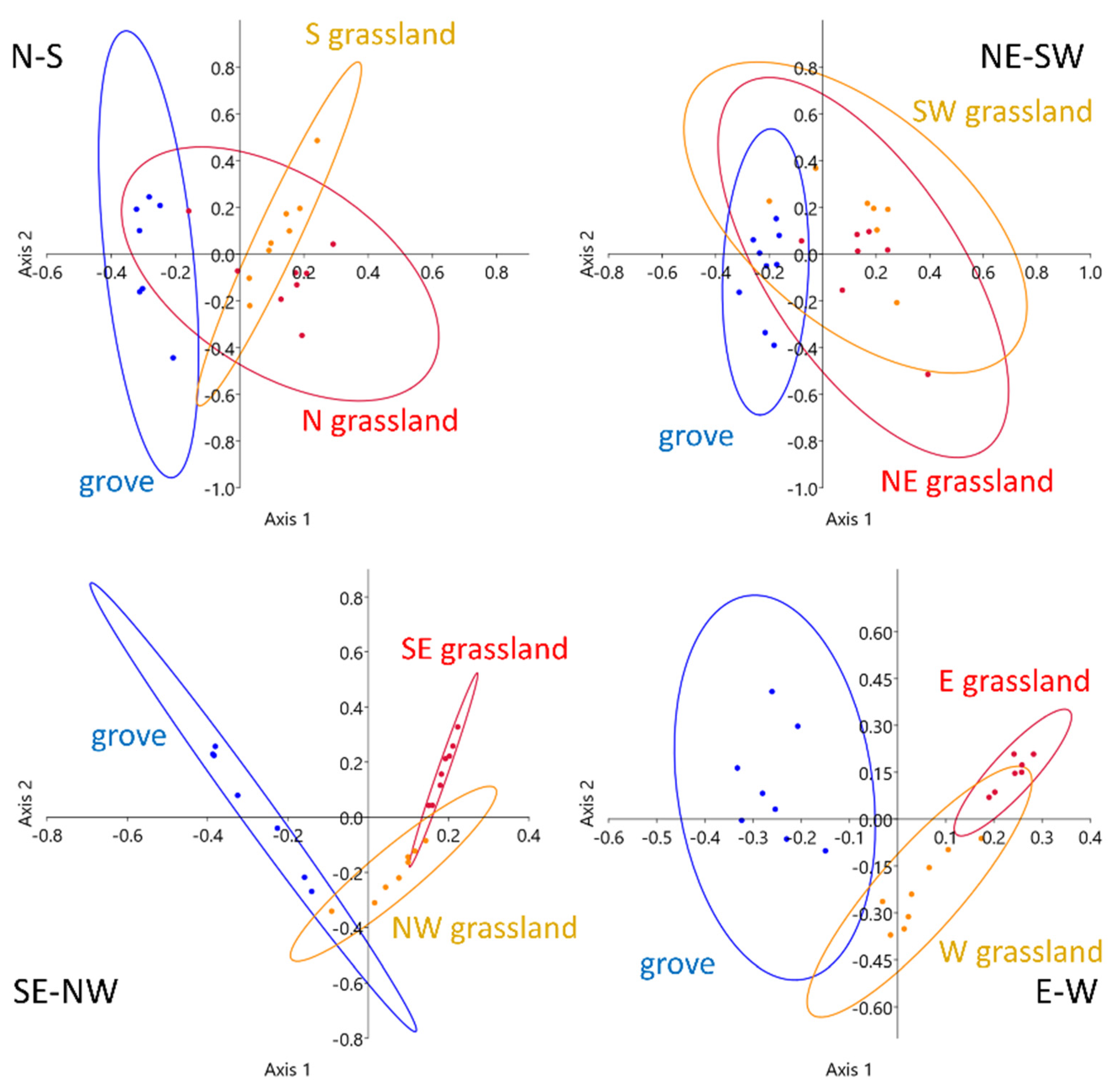
The ordinations also showed the different behaviour of the open areas of the SE–NW and E–W transects. During July, the open areas of these two transects were clearly distinct from each other, in contrast to the other two transects, where the confidence ellipses largely overlapped. The below-canopy positions were separated only in the SE–NW and E–W transects, while no outstanding differences were observed in the microclimatic conditions of the two other transects (Figure 7).
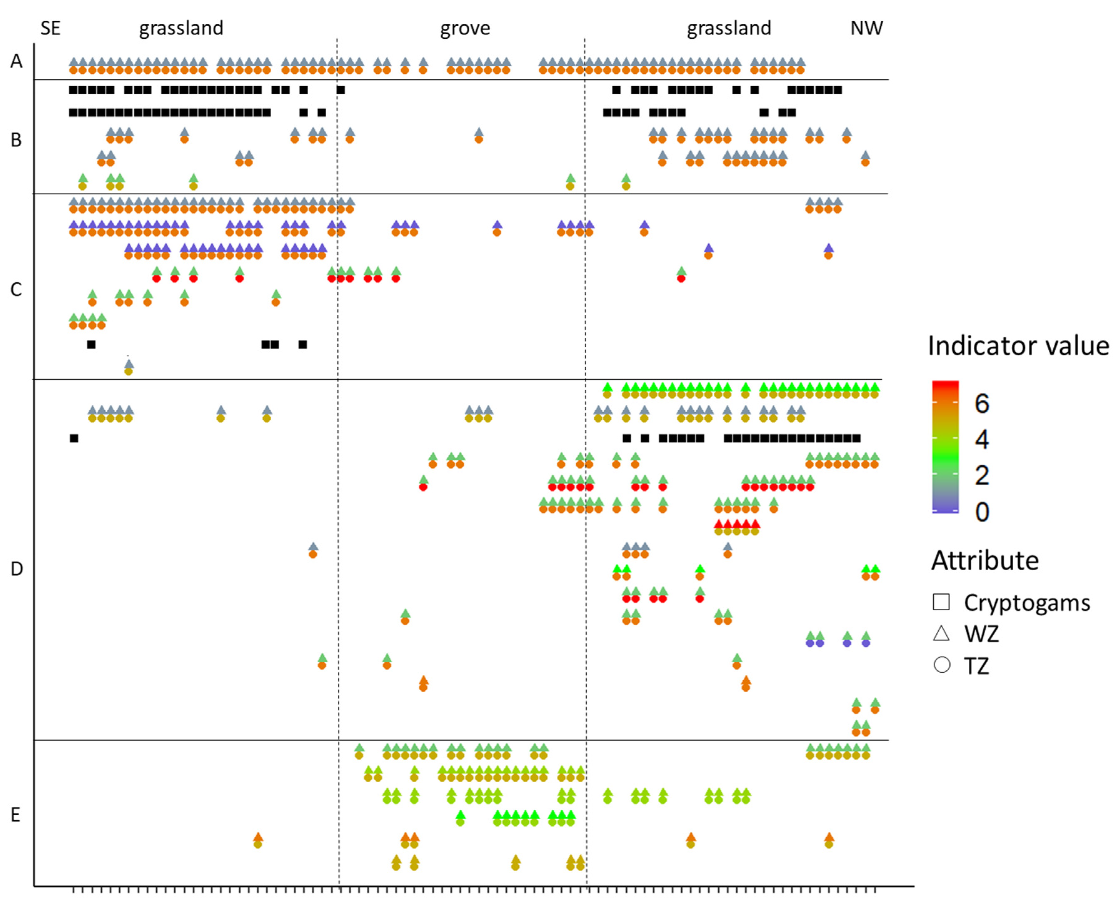
Festuca vaginata (the only species in Group A) occurred both in the grasslands and in the grove along the transect in Figure 8. Except for a few grassland species that were found on both sides of the group of trees (Group B), there were three characteristic spatial groups of species: species occurring on the south-eastern side (C) or the north-western side (D) of the grassland and species occurring mainly or exclusively in the grove (E). According to the Zólyomi-indicator values, the plant species below the canopy had a notably higher moisture and lower temperature requirement than the species in the grassland. On the other hand, there was also a difference between the species of the two grassland sides. Group C (species occurring on the south-eastern side of the grassland) had slightly lower moisture and higher temperature requirements than Group D (species occurring on the north-western side of the grassland).
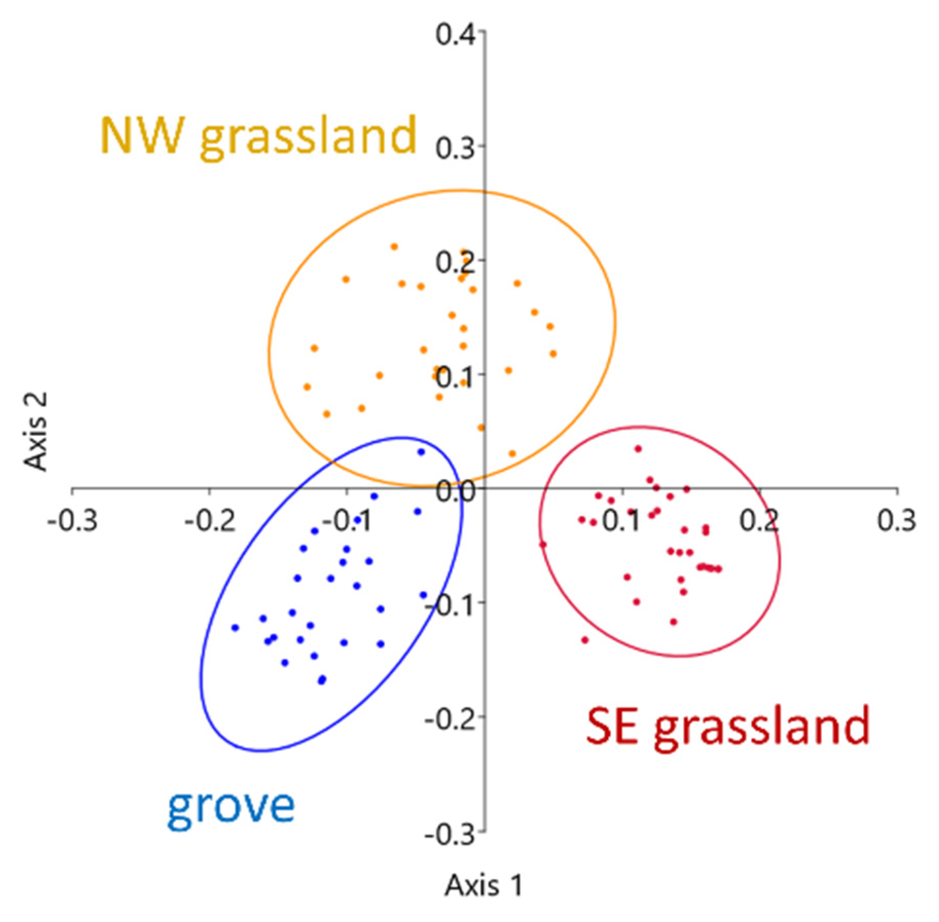
The ordination of the microcoenological data shows a clear difference between the three vegetation patches (Figure 9). The two grassland sides were notably separated from each other, and the grove just slightly overlapped with the NW grassland area. This slight overlap also applied to the VPD distribution (Figure 7, lower-left panel), indicating a more gradual transition toward the grove. The SE grassland side separated from the grove, similarly to the vegetation data, and the small overlap between the two grassland sides referred to the microclimatic similarities at the transect ends, which could also be observed in Figure 8. However, the two grassland sides showed remarkable microcoenological differences, and this difference was also manifested in the microclimatic conditions.
4. Discussion
Habitats sensitive to environmental changes, such as transition zones, have complex vegetation dynamics formed by the interaction of the biotic and abiotic factors of the two vegetation components [4]. This interaction is called an edge effect, which is manifested in the microclimatic and vegetation structural differences between the forest edge and the interior of the forest [5]. In the sandy forest-steppe habitat, the edge effect is caused by the different structural complexity of the surrounding grassland, with the outstandingly open, treeless, plain vegetation structure and low biomass [5,10,14].
To test some of the abiotic–biotic relationships for transition zones, we carried out microclimate measurements in a sandy forest-steppe habitat in Hungary. From the air temperature and air humidity measured, we calculated the vapour pressure deficit (VPD), which is an important limiting factor in plant growth, determining plant photosynthesis, because CO2 uptake is strongly limited due to stomatal closure to prevent water loss [5,22,24].
We found that during a 24-h period, microclimatic differences between grassland, edge, and below-canopy areas can be determined based on the VPD (Figure 2). The range of the VPD was significantly lower within the grove than in the open area. These results are in good agreement with previous temperature data of several other edge studies [4,5,10,13]. In the edges, we also observed a special behaviour of the VPD in that the values were higher with a more abrupt rise in the warmer edge than in the open area, which can be explained by the heat-reflecting properties of the sunny side of the tree group. However, on the colder side of the transects, in line with the shadow effect, this elevated VPD does not occur at the edges and the deficit increases with distance from the tree group. This effect was more pronounced due to the lower altitude of the Sun (October) in the eastern, south-eastern, and southern borders but also in relatively cloudy weather conditions (May).
However, the extreme values, such as the maximum and the minimum, often occur only for short periods. We introduced a new method of applying the duration curve, showing the distribution of a variable over a measurement period [34,35]. Thus, the duration of values being over a threshold provides important information about the spatio-temporal VPD pattern. In this case, the exceedance rate with respect to the critical value of 1.2 kPa calculated from the 24-h VPD DCs showed a stress effect [22,24]. The duration curve method is presented in Figure 3 for the SE–NW transect, where the difference in the effect of the exposure was the most pronounced, in contrast to that for the N–S orientation, which is referred to as the coolest–warmest gradient in other studies [4,13,20]. For example, a study [4] of the edges of an oak-chestnut forest in the U.S. showed a difference of more than 5 °C between the south and north edges at the same measurement time. Another study in a Douglas-fir forest in the U.S. [13] also observed a remarkable difference between the south and north edges in short-wave radiation and air humidity during a diurnal period. In our study, in each season, at least 20% of the values were above the threshold, indicating semi-desert conditions in this habitat [9,10]. This new method also showed an increase in the variability of the exceedance rates (Figure 3), thus highlighting the importance of examining significant differences between the parts of the study site with a higher threshold.
We also found seasonal differences among the VPD distributions: the exceedance rate was much lower in spring and autumn than in the summer measurements (Figure 4 and Figure 6). Spring and autumn did not differ significantly from each other due to the cloudy weather conditions in May. We also found differences in the VPD exceedance rate between opposite ends of the transects, which is a clear indication of the stronger stress effects in the warmer grassland areas during autumn. Choosing 3.0 kPa as the threshold value for the exceedance rate, the curves show a stronger moderating effect of the grove: a 0–10% duration of values being above 3.0 kPa in the colder grassland areas as opposed to a 25–30% duration in the warmer areas in the autumn. In the case of the above-3.0 kPa rate, this significant difference between the opposite areas showed that the distribution of the values above the threshold was notably varied within a seemingly homogeneous grassland (Figure 3 and Figure 5). Thus, our first hypothesis that the VPD-modifying effect of the grove would gradually decrease in all directions away from the edge was only partially confirmed because this modifying effect can be detected even at a distance of 6–10 meters from the edge, which is slightly different from the results of the other edge studies. Considering the small size of the grove we examined, this effect was stronger than suggested in other studies [4,5,10,13]. Our second hypothesis, which says that the spatial microclimate patterns do not differ from season to season and only the intensity of the modifying effect changes should also be rejected since the seasonal differences were also manifest in the changes in the position of the edge effect.
In the edges of the grove, we found an interesting pattern in the VPD exceedance rate (Figure 5a,c). We observed an increasing tendency from west to south-east and then a remarkable decreasing trend from south to west. However, these trends did not appear in the case of the grassland end positions (Figure 5b,d). Thus, the cardinal and intercardinal directions clearly define the characteristics of stressful conditions in the edges of the forest patches. During the summer measurements, a sharp temperature difference developed at the southern, southeastern, and eastern edges at higher altitudes of the Sun, while no pronounced edge effect was detected in the north-eastern and south-western borders. Due to the exposure and the distance from the grove, the open areas were also influenced by other parameters such as the altitude and shadows of other groves and vegetation patches. Other studies [4,20] showed that due to the larger exposure to irradiation, the south edge should differ the most from the forest interior. In the U.S., oak-chestnut forests showed a difference of at least 5 °C between the south edge and the forest interior [4]. According to our measurements, this heat gradient did not develop in summer (Figure 6b), but it was visible in the SW–NE line in autumn (Figure 6c); thus, the southern areas were not persistently the warmest in each season. Above the 3.0 kPa threshold in October (Figure 5c), in the NW, N, and NE edges, the exceedance rate was 0%, which is a good indication of the shading effect due to the lower altitude of the Sun in October. Ordinations based on the distribution of the VPD values (Figure 7) also support the microclimate-modifying effect of the grove. This effect was present in all periods, but it was most pronounced during the summer measurements. We also found clear differences between the edges based on the cardinal and intercardinal directions with this analysis, which also partially refutes our first hypothesis stating that similar trends of VPD-modifying effect can be observed in all directions from the grove.
The patterns explored highlight the importance of fine-scale sampling and analysis. Owing to our microcoenological data, we also found spatial heterogeneity in plant species distributions (Figure 8) in the open sandy grassland plant associations (Festucetum vaginatae). Except for a few grassland species that were found on both sides of the group of trees, there were three characteristic spatial groups of species: species occurring on the south-eastern side or the north-western side of the grassland and species occurring in the grove. This indicated the microclimatic differences in the study site, mostly between the grove and the surrounding, opposite grassland areas. Some species within the association behaved as differential species and indicated well the microclimatic differences in a seemingly homogeneous grassland area with a small group of trees. This distribution of plant species is a good indication of the different environmental conditions underneath even such a small group of trees. In accordance with the spatial heterogeneity of plant species distributions in our study, previous studies also showed that the forest edge may have a higher species number than the surrounding open area or the forest interior; thus, the edge acts as a transition zone with higher diversity [5,10,12,14,42,43]. In our case, the shading effect of the tree group has significant influencing power, which can be observed in the surrounding grassland. Therefore, our third hypothesis that the coenological and indication structure of the herb layer is homogeneous in the open grassland must also be rejected.
5. Conclusions
This study has provided information concerning the effects of a small group of trees on the microclimate components of a forest-steppe habitat. We observed the main characteristics and distribution of the dominant physical parameters of the abiotic edge effect [14], including the air temperature and air humidity in this habitat. The vapour pressure deficit is a susceptible indicator of the environmental conditions for vegetation. We successfully applied the duration curve method on the VPD dataset. The VPD duration curves with thresholds of 1.2 kPa and 3.0 kPa were very informative in the spatio-temporal analysis, as the VPD exceedance rate could show the stress rate for the vegetation.
The cardinal and intercardinal directions as well as the altitude of the Sun have influences on the moderating and shading effects of the grove. With distance from the grove, the effects of other parameters increase significantly. We have also shown that not only the southern area could be consistently the warmest in a natural ecosystem.
We highlighted the importance of fine-scale sampling and analysis by demonstrating that the sample positions densely spaced in a continuous transect were able to reveal significant differences within small distances, which could be important in reassessing the structure of transition zones. In addition, they can uncover the patterns within seemingly homogeneous vegetation.
This knowledge is valuable for assessing the dynamics and spatio-temporal pattern of abiotic factors and physiognomy in this type of ecosystem, which is a natural transition zone in the temperate vegetation.
Supplementary Materials
The following are available online at https://0-www-mdpi-com.brum.beds.ac.uk/1999-4907/11/10/1078/s1. Table S1: Zólyomi’s T and W scales (TZ, WZ)—relative ecological indicator values for the optimum temperature and humidity.
Author Contributions
Conceptualization, L.K. and J.B.; methodology, G.S. and L.K.; software, S.F.; sampling, G.S., B.G., and L.K.; validation, L.K.; formal analysis, G.S. and L.K.; writing—original draft preparation, G.S.; writing—review and editing, L.K., J.B., and S.F.; visualization, G.S., S.F., and L.K. All authors have read and agreed to the published version of the manuscript.
Funding
This research received no external funding.
Acknowledgments
We would like to thank the Institute of Ecology and Botany, Centre for Ecological Research, for use of the Fülöpháza research station. G.S., J.B., and S.F. acknowledge the support of the Higher Education Institutional Excellence Program (NKFIH-1159-6/2019) awarded by the Ministry of Human Capacities within the framework of water-related research of Szent István University.
Conflicts of Interest
The authors declare no conflict of interest.
References
- Von Arx, G.; Dobbertin, M.; Rebetez, M. Spatio-temporal effects of forest canopy on understory microclimate in a long-term experiment in Switzerland. Agric. For. Meteorol. 2012, 166, 144–155. [Google Scholar] [CrossRef]
- Bertrand, R.; Lenoir, J.; Piedallu, C.; Riofrı´o-Dillon, G.; de Ruffray, P.; Vidal, C.; Pierrat, J.C.; Ge´gout, J.C. Changes in plant community composition lag behind climate warming in lowland forests. Nature 2011, 479, 517–520. [Google Scholar] [CrossRef]
- Cunningham, C.; Zimmermann, N.E.; Stoeckli, V.; Bugmann, H. Growth of Norway spruce (Picea abies L.) saplings in subalpine forests in Switzerland: Does spring climate matter? For. Ecol. Manage. 2006, 228, 19–32. [Google Scholar] [CrossRef]
- Matlack, G.R. Microenvironment variation within and among deciduous forest edge sites in the eastern United State. Biol. Conserv. 1993, 66, 185–194. [Google Scholar] [CrossRef]
- Young, A.; Mitchell, N. Microclimate and vegetation edge effects in a fragmented podocarp-broadleaf forest in New Zealand. Biol. Conserv. 1994, 67, 63–72. [Google Scholar] [CrossRef]
- Baker, S.C.; Spies, T.A.; Wardlaw, T.J.; Balmer, J.; Franklin, J.F.; Jordan, G.J. The harvested side of edges: Effect of retained forests on the re-establishment of biodiversity in adjacent harvested areas. For. Ecol. Manag. 2013, 302, 107–121. [Google Scholar] [CrossRef]
- Heithecker, T.D.; Halpern, C.B. Edge-related gradients in microclimate in forest aggregates following structural retention harvests in western Washington. For. Ecol. Manag. 2007, 248, 163–173. [Google Scholar] [CrossRef]
- Kovács, B.; Tinya, F.; Ódor, P. Stand structural drivers of microclimate in mature temperate mixedforests. Agric. For. Meteorol. 2017, 234, 11–21. [Google Scholar] [CrossRef] [Green Version]
- Bodrogközy, G. Die Vegetation der Weisspappel-Haine in dem Reservat Emlékerdő bei Szeged-Ásotthalom. Acta Biol. Szeged. 1957, 3, 127–140. [Google Scholar]
- Erdős, L.; Tölgyesi, C.; Horzsea, M.; Tolnay, D.; Hurton, Á.; Schulcz, N.; Körmöczi, L.; Lengyel, A.; Bátori, Z. Habitat complexity of the Pannonian forest-steppe zone and its nature conservation implications. Ecol. Complex. 2014, 17, 107–118. [Google Scholar] [CrossRef]
- Pongrácz, R.; Bartholy, J.; Kis, A. Estimation of future precipitation conditions for Hungary with special focus on dry periods. Időjárás Q. J. Hung. Meteorol. Serv. 2014, 118, 305–321. [Google Scholar]
- Morecroft, M.D.; Taylor, M.E.; Oliver, H.R. Air and soil microclimates of deciduous woodland compared to an open site. Agric. For. Meteorol. 1998, 90, 141–156. [Google Scholar] [CrossRef]
- Chen, J.; Franklin, J.F.; Spies, T.A. Contrasting microclimates among clearcut, edge, and interior old-growth Douglas-fir forest. Agric. For. Meteorol. 1993, 63, 219–237. [Google Scholar] [CrossRef]
- Murcia, C. Edge effects in fragmented forests: Implications for conservation. Trends Ecol. Evol. 1995, 10, 58–62. [Google Scholar] [CrossRef]
- Latif, Z.A.; Blackburn, G.A. The effects of gap size on some microclimate variables during late summer and autumn in a temperate broadleaved deciduous forest. Int. J. Biometeorol. 2010, 54, 119–129. [Google Scholar] [CrossRef]
- Potter, C. Microclimate influences on vegetation water availability and net primary production in coastal ecosystems of Central California. Landsc. Ecol. 2014, 29, 677–687. [Google Scholar] [CrossRef]
- Cuena-Lombraña, A.; Fois, M.; Fenu, G.; Cogoni, D.; Bacchetta, G. The impact of climatic variations on the reproductive success of Gentiana lutea L. in a Mediterranean mountain area. Int. J. Biometeorol. 2018, 62, 1283–1295. [Google Scholar] [CrossRef]
- Hohnwald, S.; Indreica, A.; Walentowski, H.; Leuschner, C. Microclimatic Tipping Points at the Beech-Oak Ecotone in the Western Romanian Carpathians. Forests 2020, 11, 919. [Google Scholar] [CrossRef]
- Lin, B.S.; Lin, Y.J. Cooling Effect of Shade Trees with Different Characteristics in a Subtropical Urban Park. Hortscience 2010, 45, 83–86. [Google Scholar] [CrossRef] [Green Version]
- Chen, J.; Franklin, J.F.; Spies, T.A. Growing-season microclimatic gradients from clearcut edges into old-growth douglas-fir forests. Ecol. Appl. 1995, 5, 74–86. [Google Scholar] [CrossRef]
- Bolton, D. The computation of equivalent potential temperature. Mon. Weather Rev. 1980, 108, 1046–1053. [Google Scholar] [CrossRef] [Green Version]
- Novick, K.; Ficklin, D.; Stoy, P.; Williams, C.A.; Oishi, A.C.; Papuga, S.A.; Blanken, P.D.; Noormets, A.; Sulman, B.N.; Scott, R.; et al. The increasing importance of atmospheric demand for ecosystem water and carbon fluxes. Nat. Clim. Chang. 2016, 6, 1023–1027. [Google Scholar] [CrossRef] [Green Version]
- Spittlehouse, D.L.; Adams, R.S.; Winkler, R.D. Forest, Edge and Opening Microclimate at Sicamous Creek; Research Report 24; Ministry of Forests Research Branch: Victoria, BC, Canada, 2004.
- Shamshiri, R.R.; Jones, J.W.; Thorp, K.R.; Ahmad, D.; Man, H.C.; Taheri, S. Review of optimum temperature, humidity, and vapour pressure deficit for microclimate evaluation and control in greenhouse cultivation of tomato: A review. Int. Agrophysics 2018, 32, 287–302. [Google Scholar] [CrossRef]
- Shamshiri, R.R.; Kalantari, F.; Ting, K.C.; Thorp, K.R.; Hameed, I.A.; Weltzien, C.; Ahmad, D.; Shad, Z.M. Advances in greenhouse automation and controlled environment agriculture: A transition to plant factories and urban agriculture. Int. J. Agricul. Biol. Eng. 2018, 11, 1–22. [Google Scholar] [CrossRef]
- Geiger, R.; Aron, R.H.; Todhunter, P. The Climate Near the Ground; Rowman & Littlefield: Lanham, MD, USA, 2009; 623p. [Google Scholar] [CrossRef]
- Magnago, L.F.S.; Rocha, M.F.; Meyer, L.; Martins, S.V.; Meira-Neto, J.A.A. Microclimatic conditions at forest edges have significant impacts on vegetation structure in large Atlantic forest fragments. Biodivers. Conserv. 2015, 24, 2305–2318. [Google Scholar] [CrossRef]
- Connell, J.H.; Slatyer, R.O. Mechanisms of succession in natural communities and their role in community stability and organization. Am. Nat. 1977, 111, 1119–1144. [Google Scholar] [CrossRef]
- Kollmann, J. Regeneration window for fleshy-fruited plants during scrub development on abandoned grassland. Ecoscience 1995, 2, 213–222. [Google Scholar] [CrossRef]
- Wiström, B.; Nielsen, A.B. Effects of planting design on planted seedlings and spontaneous vegetation 16 years after establishment of forest edges. New For. 2014, 45, 97–117. [Google Scholar] [CrossRef]
- Körmöczi, L.; Bátori, Z.; Erdős, L.; Tölgyesi, C.; Zalatnai, M.; Varró, C. The role of randomization tests in vegetation boundary detection with moving split-window analysis. J. Veg. Sci. 2016, 27, 1288–1296. [Google Scholar] [CrossRef]
- Erdős, L.; Ambarlı, D.; Anenkhonov, O.A.; Bátori, Z.; Cserhalmi, D.; Kiss, M.; Kröel-Dulay, G.; Liu, H.; Magnes, M.; Molnár, Z.; et al. The edge of two worlds: A new review and synthesis on Eurasian forest-steppes. Appl. Veg. Sci. 2018, 21, 345–362. [Google Scholar] [CrossRef]
- FLÓRA Adatbázis 1.2 Taxonlista és Attribútum-Állomány (FLORA Database 1.2 Taxon-List and Attribute Values). Available online: https://okologia.mta.hu/node/2448 (accessed on 12 September 2020).
- Vogel, R.M.; Fennessey, N.M. Flow‐duration curves. I: New interpretation and confidence intervals. J. Water Res. Plan. Manag. 1994, 120, 485–504. [Google Scholar] [CrossRef]
- Lane, P.N.J.; Best, A.E.; Hickel, K.; Zhang, L. The response of flow duration curves to afforestation. J. Hydrol. 2005, 310, 253–265. [Google Scholar] [CrossRef]
- Verma, R.K.; Murthy, S.; Verma, S.; Mishra, S.K. Design flow duration curves for environmental flows estimation in Damodar River Basin, India. Appl. Water Sci. 2017, 7, 1283–1293. [Google Scholar] [CrossRef] [Green Version]
- R Core Team. R: A Language and Environment for Statistical Computing; R Foundation for Statistical Computing: Vienna, Austria, 2017. [Google Scholar]
- Akima, H.; Gebhardt, A.; Petzold, T.; Maechler, M. Interpolation of Irregularly and Regularly Spaced Data. R Package Version 0.6–2. 2016. Available online: https://cran.r-project.org/web/packages/akima/akima.pdf (accessed on 10 March 2020).
- Oksanen, J.; Blanchet, F.G.; Friendly, M.; Kindt, R.; Legendre, P.; McGlinn, D.; Minchin, P.R.; O’Hara, R.B.; Wagner, H. Vegan: Community Ecology Package. R Package Version 2.5–6. 2019. Available online: http://vegan.r-forge.r-project.org/ (accessed on 18 March 2020).
- Wickham, H. ggplot2: Elegant Graphics for Data Analysis; Springer: New York, NY, USA, 2016. [Google Scholar]
- Hall, C.A.; Meyer, W.W. Optimal error bounds for cubic spline interpolation. J. Approx. Theory 1976, 16, 105–122. [Google Scholar] [CrossRef] [Green Version]
- Ries, L.; Fletcher, R.J.; Battin, J.; Sisk, T.D. Ecological responses to habitat edges: Mechanisms, models, and variability explained. Annu. Rev. Ecol. Evol. Syst. 2004, 35, 491–522. [Google Scholar] [CrossRef] [Green Version]
- Erdős, L.; Török, P.; Szitár, K.; Bátori, Z.; Tölgyesi, C.; Kiss, P.J.; Bede-Fazekas, Á.; Kröel-Dulay, G. Beyond the Forest-Grassland Dichotomy: The Gradient-Like Organization of Habitats in Forest-Steppes. Front. Plant. Sci. 2020, 11, 236. [Google Scholar] [CrossRef] [Green Version]
Figure 1.
Study site (a) and relief map with the indication of the grove (b). Coordinates refer to the Hungarian Unified National Projection System. There were 89 measurement positions (4 × 22 positions in the four transects and the centre as position 12 in all transects). White dashed line: visual tree edge. Black dashed lines: the position and extent of individual shrubs and poplar sprouts.

Figure 2.
Boxplots of vapour pressure deficit (VPD) values from 24-h periods of three measurement campaigns according to the cardinal directions. Blue dashed vertical lines: visual tree edges; green horizontal lines: VPD threshold (1.2 kPa); red lines: local averages.
Figure 2.
Boxplots of vapour pressure deficit (VPD) values from 24-h periods of three measurement campaigns according to the cardinal directions. Blue dashed vertical lines: visual tree edges; green horizontal lines: VPD threshold (1.2 kPa); red lines: local averages.

Figure 3.
VPD duration curves for the SE–NW transect from three 24-h measurement periods. Blue dashed line indicates the 1.2 kPa physiological threshold; black dashed line indicates 3.0 kPa threshold, above which the exceedance rates significantly diversified.
Figure 3.
VPD duration curves for the SE–NW transect from three 24-h measurement periods. Blue dashed line indicates the 1.2 kPa physiological threshold; black dashed line indicates 3.0 kPa threshold, above which the exceedance rates significantly diversified.

Figure 4.
Exceedance (duration) (%) for VPD values above 1.2 kPa (a) and VPD values above 3.0 kPa (b) from 24-h period of three measurement periods; the left sides of the positions are the “cold” ends (W, NW, N, and NE), the right sides are the “warm” ends (E, SE, S, and SW), and the blue arrows are the centres of the transects.

Figure 5.
Exceedance rates for VPD values with respect to 1.2 kPa (top panels: (a,b)) and 3.0 kPa (lower panels: (c,d)) from 24-h period of three measurement periods; (a,c): edge positions; (b,d): grassland end positions.
Figure 5.
Exceedance rates for VPD values with respect to 1.2 kPa (top panels: (a,b)) and 3.0 kPa (lower panels: (c,d)) from 24-h period of three measurement periods; (a,c): edge positions; (b,d): grassland end positions.

Figure 6.
Spatial plots of exceedance rates (%) for VPD values with respect to 3.0 kPa from 24-h period of three measurement periods (coordinates refer to the Hungarian Unified National Projection System (m)); (a): May, (b): July, and (c): October. White dashed line: visual tree edge. Black dashed lines: the position and extent of individual shrubs and poplar sprouts.

Figure 7.
Principal coordinate analysis (PCoA) ordination of VPD quantiles in each transect in July 2018; 95% confidence ellipses are drawn according to vegetation patches.
Figure 7.
Principal coordinate analysis (PCoA) ordination of VPD quantiles in each transect in July 2018; 95% confidence ellipses are drawn according to vegetation patches.

Figure 8.
Distribution of the species along the SE–NW (Southeast–Northwest) transect in July 2018, together with the Zólyomi ecological indicator values, which quantify the temperature (TZ) and moisture (WZ) optimums for the plant species. Horizontal bars indicate coexisting species groups: (A) ubiquitous species; (B) species occurring in the grassland; (C) species occurring on the south-eastern side of the grassland; (D) species occurring on the north-western side of the grassland; (E) species occurring in the grove. List of species is shown in Table 1.

Figure 9.
PCoA ordination of microcoenological data from the SE–NW transect. Jaccard index was used on summer measurements. Ellipses representing 95% confidence are drawn according to vegetation patch.
Figure 9.
PCoA ordination of microcoenological data from the SE–NW transect. Jaccard index was used on summer measurements. Ellipses representing 95% confidence are drawn according to vegetation patch.


Table 1.
Species groups of the SE–NW transect ordered according to Figure 8. (A) ubiquitous species; (B) species occurring in the grassland; (C) species occurring on the south-eastern side of the grassland; (D) species occurring on the north-western side of the grassland; (E) species occurring in the grove; (F) low-frequency species not marked in Figure 8.
| A | Festuca vaginata |
| B | Cladonia foliacea Huds.; Tortula ruralis (Hedw.) Gaertn., Meyer, & Scherb.; Euphorbia seguieriana Neck.; Potentilla arenaria Borkh.; Artemisia campestris L. |
| C | Stipa borysthenica Klokov ex Prokudin; Dianthus serotinus Waldst. et Kit.; Fumana procumbens Gren. et Godr.; Bothriochloa ischaemum (L.) Keng; Poa bulbosa L.; Thymus pannonicus All.; Cladonia furcata (Huds.) Schrad.; Syrenia cana (Piller et Millerp.) Neilr. |
| D | Poa angustifolia L.; Gypsophila fastigiata L.; Cladonia magyarica Vain. ex Gyeln.; Carex liparicarpos Gaudin; Eryngium campestre L.; Asperula cynanchica L.; Salix rosmarinifolia L.; Centaurea arenaria M. Bieb, ex Willd.; Cynodon dactylon (L.) Pers.; Alyssum tortuosum Willd.; Thesium linophyllon L.; Equisetum ramosissimum Desf.; Tragopogon floccosus Waldst. et Kit.; Scirpoides holoschoenus (L.) Soják; Stipa capillata L.; Hieracium auriculoides Láng |
| E | Calamagrostis epigeios (L.) Roth; Crataegus monogyna Jacq.; Solidago virgaurea L.; Juniperus communis L.; Populus alba; Celtis occidentalis L. |
| F | Alkanna tinctoria (L.) Tausch; Asparagus officinalis L.; Berberis vulgaris L.; Chondrilla juncea L.; Cornus mas L.; Crepis rhoeadifolia M. Bieb.; Cynoglossum officinale L.; Euphorbia cyparissias L.; Galium mollugo L. s. str.; Helianthemum canum (L.) Hornem.; Leontodon autumnalis L.; Medicago minima (L.) L.; Polygonum arenarium Waldst. et Kit.; Taraxacum officinale F.H.Wigg; Teucrium chamaedris L.; Tragus racemosus (L.) All. |
© 2020 by the authors. Licensee MDPI, Basel, Switzerland. This article is an open access article distributed under the terms and conditions of the Creative Commons Attribution (CC BY) license (http://creativecommons.org/licenses/by/4.0/).
Share and Cite
MDPI and ACS Style
Süle, G.; Balogh, J.; Fóti, S.; Gecse, B.; Körmöczi, L. Fine-Scale Microclimate Pattern in Forest-Steppe Habitat. Forests 2020, 11, 1078. https://0-doi-org.brum.beds.ac.uk/10.3390/f11101078
AMA Style
Süle G, Balogh J, Fóti S, Gecse B, Körmöczi L. Fine-Scale Microclimate Pattern in Forest-Steppe Habitat. Forests. 2020; 11(10):1078. https://0-doi-org.brum.beds.ac.uk/10.3390/f11101078
Chicago/Turabian StyleSüle, Gabriella, János Balogh, Szilvia Fóti, Bernadett Gecse, and László Körmöczi. 2020. "Fine-Scale Microclimate Pattern in Forest-Steppe Habitat" Forests 11, no. 10: 1078. https://0-doi-org.brum.beds.ac.uk/10.3390/f11101078
Note that from the first issue of 2016, this journal uses article numbers instead of page numbers. See further details here.