Article

Spatially Explicit Analysis of Trade-Offs and Synergies among Multiple Ecosystem Services in Shaanxi Valley Basins

1
School of Geography and Tourism, Shaanxi Normal University, Xi’an 710119, China
2
College of Geomatics, Xi’an University of Science and Technology, Xi’an 710054, China
*
Author to whom correspondence should be addressed.
Submission received: 12 January 2020 / Revised: 3 February 2020 / Accepted: 7 February 2020 / Published: 12 February 2020

Abstract

:
Understanding the spatiotemporal characteristics of trade-offs and synergies among multiple ecosystem services (ESs) is the basis of sustainable ecosystem management. The ecological environment of valley basins is very fragile, while bearing the enormous pressure of economic development and population growth, which has damaged the balance of the ecosystem structure and ecosystem services. In this study, we selected two typical valley basins—Guanzhong Basin and Hanzhong Basin—as study areas. The spatial heterogeneity of trade-offs and synergies among multiple ESs (net primary production (NPP), habitat quality (HQ), soil conservation (SC), water conservation (WC), and food supply (FS)) were quantified using the correlation analysis and spatial overlay based on the gird scale to quantitatively analyze and compare the interaction among ESs in two basins. Our results found that: (1) Trade-offs between FS and other four services NPP, HQ, SC, and WC were discovered in two basins, and there were synergistic relationships between NPP, HQ, SC, and WC. (2) From 2000 to 2018, the conflicted relationships between paired ESs gradually increased, and the synergistic relationship became weaker. Furthermore, the rate of change in Guanzhong Basin was stronger than that in Hanzhong Basin. (3) The spatial synergies and trade-offs between NPP and HQ, WC and NPP, FS and HQ, SC and FS were widespread in two basins. The strong trade-offs between pair ESs were widly distributed in the central and southwest of Guanzhong Basin and the southeast of Hanzhong Basin. (4) Multiple ecosystem service interactions were concentrated in the north of Qinling Mountain, the central of Guanzhong Basins, and the east of Hanzhong Basin. Our research highlights the importance of taking spatial perspective and accounting for multiple ecosystem service interactions, and provide a reliable basis for achieving ecological sustainable development of the valley basin.

Graphical Abstract

1. Introduction

Ecosystem services (ESs) are the benefits that people derive from ecosystems [1,2,3] and include four categories (supporting, regulating, provisioning, and cultural services). According to the Millennium Ecosystem Assessment (MEA) reported, 60% of worldwide ecosystem services have degraded or been in an unsustainable state because of the rapid economic development and global population growth. Therefore, it is urgent to improve the capacity of ESs by improving the eco-management measures to maintain social and economic sustainable development [4].
Due to the diversity of ecosystem services, the heterogeneity of the spatial distribution and the selectivity of human use, the multiple relationships between ecosystem services show the dynamic variation under the influence of natural factors and human activities, which are characterized by different patterns such as trade-offs and synergies [5]. Trade-offs are the situations where one service increases at the cost of another services [6,7,8]. Such as, in an agricultural system, increasing fertilizer use to improve crop yields may have significant negative effects on water purification, and indirectly decrease fishery and recreational values [9]. Synergies are the reverse of trade-offs, which can be defined as situations in which both services either increase or decrease [6]. For instance, increasing net primary productivity simultaneously increases the values of water yield and soil conservation [10]. In addition, the ecosystem has diverse functions and, thus, provide multi-level services to humans. The multiple relationships of the ecosystem service is a challenge for local ecological management [11]. Moreover, trade-offs and synergies between ESs can differ in different regions because of landscape heterogeneity across the region, and the interactions between ESs would behave in diverse ways during different periods [12]. At the same time, the distinct ecosystem management strategies of the local region may also cause various interactions among multiple ESs. Therefore, identifying trade-offs and synergies between the ecosystem service could provide a powerful message to policy makers, and better inform management choices to achieve a “win-win” situation [13,14].
The identification of trade-offs and synergies between ecosystem services can be conducted through the methods: statistical analysis [15,16,17], mapping comparison [18,19], model simulation [20,21], and scenario analysis [22,23]. In this, correlation statistical analysis is a common method used in trade-off and synergy analysis, which can usually be used in combination with other methods. By spatial correlation analysis and calculating the changes of the relationship between ESs, which can quantitatively reveal the relationship between ESs within a certain period. However, there are still some limitations in previous studies, such as trade-off and synergy analysis. These are mostly based on quantitative statistical analysis, lack of dynamic trend changes of relationships between ES for long time series, and mostly consider the pairwise interactions between ES [10,24] while neglecting the study of multiple ecosystem service interactions. Furthermore, to local ecological management, policymakers need to know the location of trade-offs and synergies among multiple ESs. Therefore, spatial explicit analysis of trade-offs and synergies will be the core research in the future study of an ecosystem service.
With global population growth and rapid economic development, urbanization has brought a great threat to local ecological environments. The expansion of urban land, the influx of migrant populations, the reduction of carbon storage and soil degradation, which have occurred in the typical valley basins [4], Yanhe Watershed [25], Guanzhong-Tianshui economic region [26], and Grain-for-Green Programme region [27], are the relevant examples. Guanzhong Basin and Hanzhong Basin is located in the central and south of Shaanxi Province, respectively, as typical Shaanxi valley basins, which are sensitive to climate change, natural disaster, landscape fragmentation, and rapid degeneration of biodiversity [24]. In addition, Guanzhong Basin and Hanzhong Basin is located on either side of Qinling Mountains, which is the geographical boundary of northern and southern of China. Therefore, they have clear differences of the natural environment and social development.
Therefore, we used the Guanzhong Basin (as an economically developed region) and Hanzhong Basin (as the ecological environment region), as case study areas to explore the temporal and spatial variations of trade-offs and synergies among multiple ecosystem services and compare the region difference. Based on five ESs (net primary production (NPP), habitat quality (HQ), soil conservation (SC), water conservation (WC), food supply (FS)) from 2000 to 2018, the identification of trade-offs, and synergies between paired ESs and correlation coefficients were calculated by spatial statistical analysis. Meanwhile the spatial distributions of multiple interactions among ESs were classified by spatial overlay analysis based on the gird cell. Then, we compare the difference of trade-offs and synergies between Guanzhong Basin and Hanzhong Basin, in order to provide a theoretical basis for ecological management decisions in Northwestern China.

2. Materials and Methods

2.1. Study Area

The Guanzhong Basin and Hanzhong Basin both belong to Shaanxi Province located in the middle part of inland China. Considering the unification of natural data and social statistical data, we used an administrative boundary to divide the Guanzhong Basin and Hanzhong Basin as study areas (Figure 1). Guanzhong Basin is located between the Loess Plateau and the Qinling Mountain. The region is between 33°35′ N and 35°51′ N and between 106°19′ E and 110°36′ E. The terrain is low in the west and high in the east. Meanwhile, Weihe River (a tributary of the Yellow River) runs through the central region, which forms a large area of alluvial plain. The Guanzhong Basin is a warm temperate zone with a semi-humid climate, distinct four seasons, hot and rainy summer, and cold and dry winter, which has diverse vegetation types and agrotypes. It is the important part of national and western economic and an ecological balanced development strategy base [28]. With the rapid development of economy, it has attracted much influx of external population until 2017. The total population was approximately 23.94 million. The GDP was 1409.20 billion and accounted for 64.35% of Shaanxi Province. The ecological environment is greatly damaged by human activities.
Hanzhong Basin is located between Qinling Mountain and Daba Mountain (geographical coordinate is 32°08′54″ N~33°53′16″N, 105°30′50″E~108°16′45″E). While the Han River (a tributary of the Yangtze River) runs through the whole region, the terrain is gradually decreasing from northwest to southeast. The Hanzhong Basin is a typical north subtropical monsoon climate zone. The climate is often mild and humid, and there is no chilly winner and there is a hot summer. Species diversity is rich and it has a fine ecological environment. The forest coverage rate is 52%, the vegetation coverage rate of forest and grass is up to 60%, and it has the reputation of “Land of Fish and Rice” and “Land of Abundance.” By 2017, the GDP was 133.33 billion, the population was 3.44 million, the crop areas were 2102.10 km2, and the grain yield reached 1.04 million tons. The region agriculture output contributes to more than 20% of the gross output. The level of economic development is low.

2.2. Data Sources

The data used in this study were obtained using the following sources.
(1) The land use/cover map in 2000 with a spatial resolution of 30 m × 30 m were applied from the Cold and Arid Region Sciences Data Center (http://westdc.westgis.ac.cn), 2005 and 2017 were provided by National Earth System Science Data Sharing Infrastructure (http://www.geodata.cn), 2010 and 2018 were down from Resource and Environment Data Cloud Platform (http://www.resdc.cn). The land use/cover data both covered six primary types and 25 secondary land use types. According to the actual land use settings in Shaanxi Province, and the need for quantitative evaluation of ecosystem services, the land cover types were classified into the following six categories: (1)Crop land, including plain dryland and irrigated land, mainly for agricultural cultivation. (2) Forest land, containing closed forest land, shrubbery, sparse wood land, and other forest land. (3) Grass land, referring to high, middle, and lower cover grassland. (4) Water area, including lake, river, reservoirs, and ponds, bottomland. (5) Settlements, containing urban land, rural residential area, industrial and mining, and other conservation land. (6) Unused land, which is currently unused and may be hard to use, including sand, bare land, swale land, saline land, and others.
(2) Digital elevation model with a resolution of 30 m was used to calculate the terrain factors in the Revised Universal Soil Loss Equation (RUSLE) model, which are available for download at Geospatial Data Could Platform (http://www.gsclooud.cn).
(3) The soil and vegetation type map of Shaanxi Province were extracted from 1:1,000,000 soil and vegetation database of China, respectively. Those were used to compute the soil conservation and net primary production, which were obtained from the National Earth System Science Data Sharing Infrastructure (http://www.geodata.cn).
(4) The Normalized Difference Vegetation Index (NDVI) was divided from the MOD13A2 product synthesized by the Maximum Value Composite (MVC) Method 16d and downloaded from the United States Geological Survey with a spatial resolution of 250 m (http://ladsweb.modaps.eosdis.nasa.gov).
(5) Meteorological data was obtained from the China Meteorological Science Data Sharing Service System (http://data.cma.cn), including average temperature, precipitation, wind speed, average air pressure, maximum temperature, minimum temperature, sunshine duration, solar radiation and more. Furthermore, via ArcGIS software using the Kriging interpolation method, we obtained the meteorological raster dataset.
(6) Major food productions, population, and gross domestic product were obtained from the Shaanxi statistical yearbooks and some statistical yearbooks from Hanzhong City and other cities from 2000 to 2018.

2.3. Quantifying Ecosystem Services

2.3.1. Net Primary Productivity (NPP)

Net Primary Productivity (NPP) is defined as the amount of organic energy produced by plant photosynthesis minus the energy consumed through autotrophic respiration [29]. This paper uses the Carnegie-Ames-Stanford approach (CASA) mode to estimate the value of NPP(net primary production) [30]. The formula is below.
N P P ( x , t ) = A P A R ( x , t ) × ε ( x , t )
where NPP (x, t) represents the net primary productivity of pix x during month t (g C·m−2·month−1), ε(x, t) describes the light utilization efficiency of pix x during month t (g C·MJ−1), and APAR(x, t) is the absorbed photosynthetically active radiation(MJ·m−2).

2.3.2. Habitat Quality (HQ)

Habitat quality refers to the ability of the ecosystem to provide conditions appropriate for individual and population persistence, and it depends on a habitat’s proximity to human land uses and the intensity of these land uses [31,32]. InVEST models’ habitat quality as a proxy for biodiversity, ultimately, estimates the extent of the habitat across the landscape, and their state of degradation [15]. The model integrates information on land use and threats to biodiversity to produce the habitat quality map [33]. The habitat quality of each grid is indicated by habitat suitability (value range from 0 to 1, 1 indicates the highest suitability of the habitat, while areas on the landscape that are not habitat get a quality score of 0) and habitat degradation. There are four factors in the function: each threat’s relative impact, the relative sensitivity of each habitat type to each threat, the distance between habitats and sources of threats, and the degree to which the land is legally protected [34]. In this study, threats included urban land, rural residential areas, and industrial and mining construction land and cropland. Moreover, the impact of these four threats on habitat decreased as the distance from the degradation source increases. Now, we choose a linear distance-decay function to describe how a threat decays over space. The impact of threat r that originated in gird cell y, ry, on habit in gird cell x is given by irxy, and the quality of the habitat in parcel x that was in LUCC j is given by Qxj and was represented by the following equations.
i r x y = 1 ( d x y d r max ) if   linear
i r x y = exp { ( 2.99 d r max ) d x y } if   exponential
Q x j = H j ( 1 ( D x j z D x j z + k 2 ) )
where r was the threat source of habitat, dxy is the linear distance between grid cells x and y, drmax is the maximum effective distance of threat r‘s reach across space, Hj indicates the habitat suitability of LULC type j, Dxj is the total threat level in grid cell x with LULC j, and z (we hard code z = 2.5) and k are scaling parameters, which are half of the maximum degradation. Furthermore, the sensitivity of different threat sources for land use is based on the InVEST 3.2.0 user’s guide and other previous studies [26,35].

2.3.3. Water Conservation (WC)

Water conservation affects the ecosystem process and crop production through various land covers. Region rainfall, evapotranspiration, storage, and sorption are vegetation processes. Water conservation is integrated as the performance of water circulation and a different natural ecosystem, such as forest, vegetation coverage, and soil. We calculated water conservation through the summation of canopy interception, litter absorption, and soil storage.
Q = Q 1 + Q 2 + Q 3
In the above equation, Q indicates the total amount of water retention capacity (t·year−1). Q1, Q2, and Q3 indicates the amount of vegetation canopy interception (t·year−1), the amount of the litter retention capacity (t·year−1), and the interception amount of the soil layer (t·year−1).
Q 1 = ( α i × β i × S i )
Q 2 = ( ε i × γ i × S i )
Q 3 = ( p i × h i × S i )
where αi is the annual rainfall (mm), βi is the canopy retention (%), Si is the area of vegetation type (ha), εi is the litter dry weight (t/ha), γi is the maximum water holding capacity (%), pi is the soil non-capillary porosity (%), and hi is soil thickness (mm) [36,37].

2.3.4. Soil Conservation (SC)

The Revised Universal Soil Loss Equation (RUSLE) is most widely used to calculate the average annual soil loss from each pixel of land. Based on the soil erosion theory and natural runoff observational data, the RUSLE model is applied using GIS software with some factors, including meteorological station dataset, the NDVI (normalized difference vegetation index) dataset, soil surveys, topographic maps, and land use data [38,39]. Therefore, the soil conservation is estimated from the difference between potential soil erosion and actual soil erosion [40].
A m = R × K × C × L S × P
A p = R × K × L S
A c = A p A m
In the above formula, Am is the amount of actual soil erosion (t·ha−1·year−1), Ap is the potential soil erosion (t·ha−1··year−1), Ac is the amount of soil conservation (t· ha−1··year−1), R is the rainfall erosivity factor, and K is the soil erodibility factor, which indicates the physical and chemical properties of soil. C is a dimensionless crop management factor. LS includes the slope length factor (L) and the slope factor (S). P is the soil conservation measures factor, which reflects people using different protection measures to prevent soil erosion of various land use types.

2.3.5. Food Supply (FS)

Food supply services are one of the most important provisioning services in agricultural ecosystems [41]. Food is the most basic material that humans obtain from the natural ecosystem, which plays a decisive role in social development [42]. In this study, we use the land use dataset and region statistical yearbook data to estimate the total food supply of each land use in the study area, in order to realize the spatialization of the food supply. The equation is as follows.
G i = A i × N i
In the above equation, Gi is the amount of ith food for each pixel. Ai is the ith food area (km2). The study area was divided into the unit grid of 1 km×1 km which is equal to 1km2. Ni is the yield of ith food for the unit area (t/km2).
N i = F i S i
where Fi is the total yield of food in the study area (t·year−1). Si is the total area of the ith food (km2) in this research, which represents the area of each land use type. Among this, the grain, oil-bearing, and vegetables belong to the cropland. The output of meat and milk belong to the grassland. The aquatic products belong to the water area.

2.4. Spatial Correlation Analysis

The spatial statistical mapping method based on correlation coefficients on a pixel scale are used to quantify the relationship between ecosystem services. This method could explore the continuous temporal changes of various ecosystem services. Meanwhile, the relationship between ESs can be spatially expressed by quantitative mapping. In this paper, the correlation coefficient for each pair of ecosystem services is calculated by ArcGIS software (ArcGIS 10.2) at a pixel scale [25]. Furthermore, the correlation coefficients of two time series based on each pixel were calculated by Spearman’s coefficient. Its expression is shown below.
r x y = i = 1 n i = 1 n ( x i j x ¯ ) ( y i j y ¯ ) i = 1 n ( x i j x ¯ ) 2 i = 1 n ( y i j y ¯ ) 2
where rxy is the spatial correlation coefficient, with values ranging from −1 to 1. If rxy > 0, represents the positive correlation between two variables, which indicates that the two services are synergistic. If rxy < 0, represents the negative correlation between two variables, which means there are trade-offs between two services. xij, yij indicates gird values for different types of ecosystem service spatial datasets.

3. Results

3.1. Spatial Distributions of Ecosystem Services

Figure 2 depicts spatial distribution of average ecosystem services in the two areas of study. In Guanzhong Basin, the average of NPP was 6.25 t·ha−1·a−1, the higher value of NPP was concentrated in the southwest, and the lowest was observed in the middle of the basin. While in Hanzhong Basin, the average of NPP is 8.21 t·ha−1·a−1, which is more than the Guanzhong Basin. The higher HQ was distributed in the northern Qinling mountain, which aggregated in forestland in the Guanzhong Basin. The average of HQ was 0.45 in the Guanzhong Basin, and 0.55 in the Hanzhong Basin. Moreover, the distribution of WC varied greatly in the Guanzhong Basin. Areas with high water conservation (WC) were concentrated in the north of Qinling Mountain and the southern of Xi’an City. It showed a clear trend from low in the north to high in the south in the Hanzhong Basin. Areas with high soil conservation (SC) were in the southwest of the Guanzhong Basin, but the central of the basin was mainly concentrated in crop land with low SC. Moreover, it could be seen the lower SC was in the central of the Hanzhong Basin, and lowest SC was just 0.01 t·ha−1·a−1. The highest value reached 1270 t·ha−1·a−1. Furthermore, the higher FS was mostly observed in the central region of the Guanzhong Basin, concentrated in farmland. The low values were in the southwest of Baoji City and most areas of the Tongchuan City. In the Hanzhong Basin, the food supply of crop land in the middle region was relatively higher, and those with low FS were distributed in the northern and southeastern basin, which are concentrated on forest land.

3.2. Spatial Correlations between Ecosystem Services

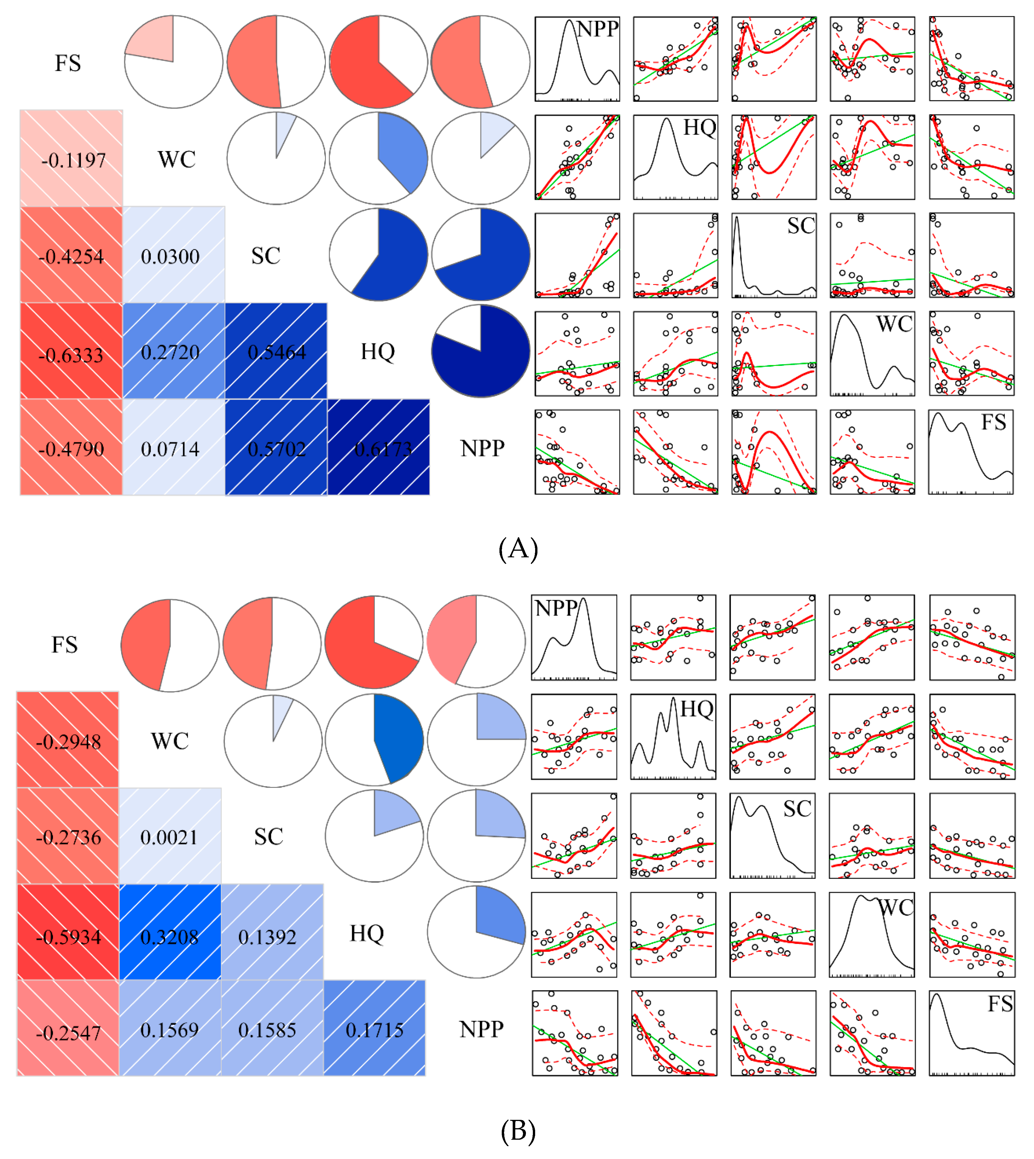
3.2.1. Trade-Offs and Synergies Analysis

We used the correlation analysis function to explore the trade-offs and synergies between each ES (Figure 3). In two basins, we could find that food supply (FS) with the other four services (soil conservation (SC), net primary productivity (NPP), habitat quality (HQ), and water conservation (WC)) both had negative relationships. While the negative relationships between FS and HQ were stronger than others, the correlation coefficient was −0.6333 and −0.5934 in the Guanzhong Basin and the Hanzhong Basin, respectively. In addition, NPP, HQ, SC, and WC presented positive relationships, and positive relationships between NPP and HQ were bigger in the Guanzhong Basin, where the correlation coefficient was up to 0.6173. The relationship between WC and SC was weak with only 0.03 and 0.002 in the Guanzhong Basin and the Hanzhong Basin, respectively. At the same time, in the scatterplot, as the FS changed, the other four ESs changed in opposite directions, while WC, HQ, NPP, and SC both had a consistent trend. Consequently, the trade-offs and synergies were identified by the correlation coefficient and the correlation diagram. The results indicated that trade-offs between FS and the other four services (NPP, HQ, SC, and WC) were discovered in two basins, and there were synergic relationships between NPP, HQ, SC, and WC. It could be explained that strong capacity of carbon storage and water retention was concentrated in forest land and grass land, but the food production was low. While the food production was bigger in cropland, the value of NPP and soil conservation was smaller. Moreover, because cropland is a core threat source of habitat quality, the habitat quality was low, which caused trade-offs between the food supply and habitat quality. When comparing the differences between the two basins, the trade-off between FS and NPP was clear in the Gunanzhong Basin. The correlation coefficient was −0.4790. While the synergy between WC and HQ was evident in theHanzhong Basin, the correlation coefficient was 0.3208. Consequently, the relationships between ecosystem services in Guanzhong Basin were more complex than those in the Hanzhong Basin. The trade-offs between FS and HQ, NPP, and SC were stronger in the Guanzhong Basin.

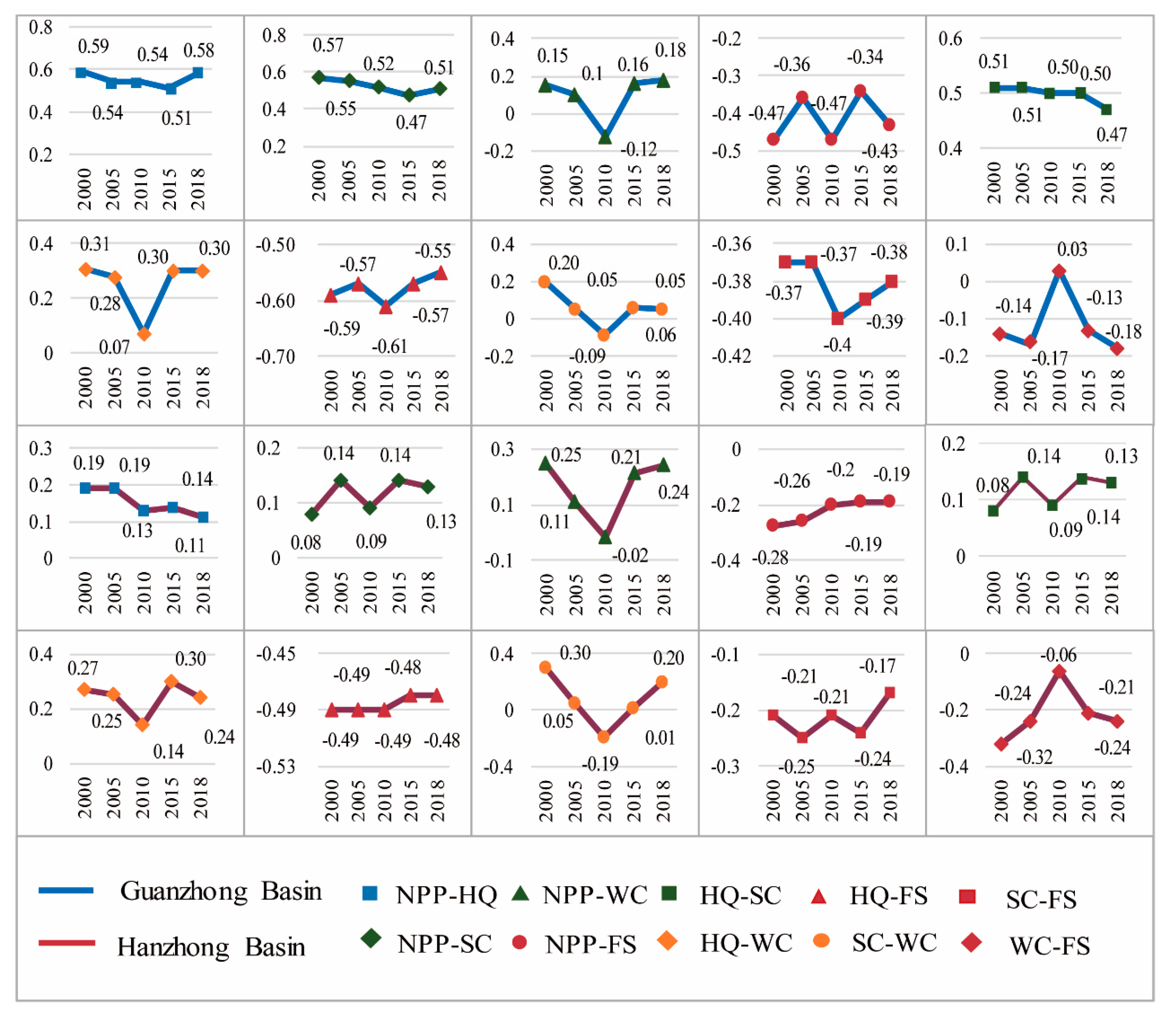
3.2.2. Temporal Analysis of Trade-Offs and Synergies

Trade-offs and synergies between ecosystem services at different periods varied greatly. We further explored the temporal changes of trade-offs and synergies from 2000 to 2018 (Figure 4). In the Guanzhong Basin, there was a stable decrease of the synergistic relationship between NPP and HQ, NPP and SC, and HQ and SC. While the relationship between NPP and WC, HQ and WC, SC and WC presented a sudden drop in 2010, even between NPP and WC, SC and WC appeared to have negative relationships. From the temporal variations of correlation coefficients, it could be seen that WC increased with the decreasing trend of NPP in 2010. Some areas of the forest increased as the crop land and grassland decreased, which might increase the conflict between WC, NPP, and SC. The trade-offs between FS and other four ESs showed a fluctuating change during this period. Compared with 2000, the negative relationship between HQ and FS has decreased, whereas the trade-off between FS and WC became strong in 2010. In the Hanzhong Basin, the positive relationship between NPP and HQ presented an evident decreasing trend. It also discovered the relationship between NPP and WC, SC and WC appeared to have a decreasing trend in 2010. Moreover, the negative relationship between WC and FS was weaker. While the conflict relationship between NPP and FS, SC and FS decreased. Therefore, we found the synergistic relationship became weak as it changed and presented a decreasing trend in the Guanzhong Basin, which presented to be somewhat stronger than those in the Hanzhong Basin. On the other hand, the trade-offs between FS and SC, FS and WC were strong in the Guanzhong Basin and the conflicted relationship became more pronounced. On the whole, the change trend of the trade-off relationship in the Guanzhong Basin was slightly faster than that in the Hanzhong Basin.

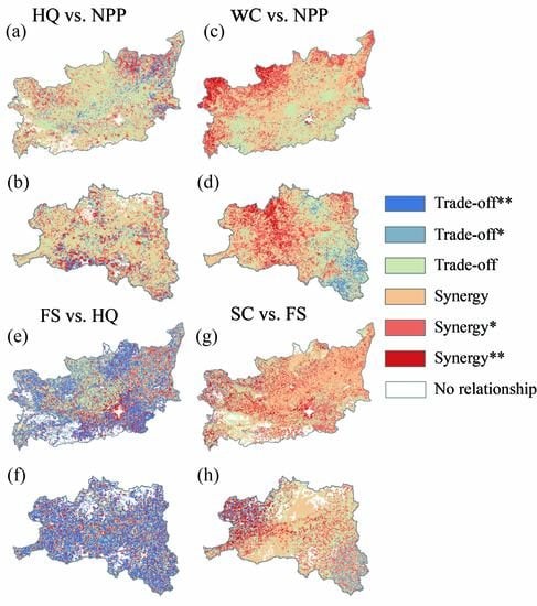
3.3. Spatial Heterogeneity of Paired Ecosystem Service Interaction Based on the Grid Scale

Through the above study, we found that the multiple interactions among ES were different and had clear temporal and spatial characteristics. The spatial correlation coefficients based on the gird from 2000 to 2018 were shown in Figure 5, which were checked according to significance (p < 0.05). In this paper, we calculated spatial correlation coefficients between regulating and supporting services as well as provisioning and regulating services. Since this study involved five different services in two regions, we took four pairs services (HQ and NPP, WC and NPP, FS and HQ, FS and SC) with good correlation, as an example.
For HQ (habitat quality) and NPP (net primary production) (Figure 5a), the strong synergies (p < 0.01 and p < 0.05) were spatially aggregated in the north-east of Weinan City and the western region of the Guanzhong Basin, mostly concentrated in the forest land, which nearly accounted for 17.83%. Strong trade-offs (p < 0.01 and p < 0.05) account for 3.40%, which were in the south-east of Weinan City and the central region of the basin. At the same time, the strong synergies (p < 0.01 and p < 0.05) were mostly found in the edge of the Hanzhong Basin, which accounted for 20.93%, while the strong trade-offs accounted for 10.31% of the land use types that were in the central region of the basin and in the southeast of the Ningqiang County (Figure 5b).
For WC (water conservation) and NPP (Figure 5c), the average spatial correlation coefficient during 2000–2018 was 0.14 with a standard deviation of 0.34. Strong synergies (p < 0.01 and p < 0.05) were spatially aggregated in the northern edge of the Guanzhong Basin, which accounted for 26.44%, mostly discovered in the forest land. Strong trade-offs (p < 0.01 and p < 0.05) that accounted for 0.81% of the land use types were in the central region of the Xi’an City. Meanwhile, in the Hanzhong Basin, the average spatial correlation coefficient was 0.07 with a standard deviation of 0.44 from 2000-2018. Strong synergies (p < 0.01 and p < 0.05) were accounted for 28.91%, which were concentrated in the north-east and Mian County. The strong trade-offs (p < 0.01 and p < 0.05) were discovered in the west-south of the basin region and Zhenba County, which accounted for 0.82% (Figure 5d).
For FS (food supply) and HQ (Figure 5e), the trade-off relationships were widespread in two basins. In the Guanzhong Basin, the average spatial correlation coefficient during 2000–2018 was −0.30 with a standard deviation of 0.64. Strong trade-offs (p < 0.01 and p < 0.05) were spatially aggregated in the surrounding areas of the Guanzhong Basin and the edge of the bigger city (e.g., crop land and grass land) accounted for 46.94%. The strong synergies (p < 0.01 and p < 0.05) accounted for 21.20% of the land use types that were in the north-east of the basin and the central of Xian City. While the average spatial correlation coefficient during 2000–2018 was −0.40 with a standard deviation of 0.68 in the Hanzhong Basin (Figure 5f). It could be seen that the trade-offs widely exited in the edge of the basin and the strong trade-offs were approximately 57.46%. The strong synergies accounted for 20.17% of the land use types in the central region of the Hanzhong Basin and the settlements around the bigger county.
For SC (soil conservation) and FS (Figure 5g), the strong trade-offs (p < 0.01 and p < 0.05) were concentrated on the north-west region of the Guanzhong Basin and the north region of the Qinling Mountain (mostly concentrated on the forest land). While strong synergies (p < 0.01 and p < 0.05) accounted for 30.12%, which were in the central area of the basin and the north-east of Weinan City, which concentrated on the crop land. Furthermore, strong trade-offs were spatially aggregated in the south-west of the Hanzhong Basin and in grassland, which accounted for 9.56% of the whole basin. Strong synergies were aggregated in the northwest and the central region of the basin, which was concentrated in the grassland (Figure 5h).

3.4. Multiple Interactions among Ecosystem Services

3.4.1. Spatial Explicit Analysis of Multiple ESs Interactions

Figure 6 depicts the multiple interactions among ES from the perspective of the valley basin as a whole unit (the detailed method was seen in Appendix A). The relationship among multiple ESs in the Guanzhong Basin varied greatly. The complex relationships were discovered in the central region of the basin and the northern Qinling Mountain. In the Guanzhong Basin, the FS gradually decreased, while NPP, HQ, SC, and WC showed a simultaneous continuous increase from 2000 to 2018. This phenomenon meant that NPP, HQ, SC, and WC had synergistic interactions, and the four services had trade-off interactions with FS. It occurred in the west of Baoji City and the north of Xianyang City, which accounted for 8.31%. SC and FS simultaneously decreased, and NPP, HQ, and WC showed continuous increases. This result indicated the synergistic interaction occurred among NPP, HQ, and WC, and had trade-offs with SC and FS. It was greatly aggregated in the edge of the basin concentrated on grassland, which accounted for 4.21%. NPP, SC, and WC showed a simultaneous continuous increase, while HQ and FS showed a simultaneous decrease. This phenomenon declared that synergistic interactions occurred among NPP, SC, and WC, and these three services showed trade-offs with HQ and FS, which accounted for 4.88% in the north of Tongchuan City and the forest land around the bigger city. NPP and FS continuously increased, and HQ, SC, and WC simultaneously underwent a continuous decrease throughout these years. Synergies occurred among NPP and FS, and two services exhibited trade-offs with HQ, SC, and WC. This phenomenon accounted for 5.45% of the whole region was in the east of Xi’an City (Figure 6A) and the southeast of Baoji City. Furthermore, the NPP gradually increased, and HQ, SC, WC, and FS simultaneously underwent a continuous decrease from 2000 to 2018. Trade-offs occurred among NPP and those four services accounted for 4.98%, which were in the northern margin of the Qinling Mountain (Figure 6B).
In the Hanzhong Basin, the relationship between multiple ESs was fairly simple than Guanzhong Basin but showed evident spatial differences. The trade-offs among FS and other four services (NPP, HQ, SC, WC, which simultaneously increased, suggesting synergies) was aggregated in the northwest of the basin accounting for 6.88% of all land use types (Figure 6C). NPP and HQ showed a simultaneous continuous increase, and SC, WC, and FS showed a simultaneous continuous decrease. It indicated that NPP and HQ had a synergistic relationship, and both presented trade-offs with the other three services (SC, WC, and FS). This phenomenon accounted for 5.89% of land use types that were in the southeast of the basin. HQ and WC showed a simultaneous continuous decrease, and NPP, SC, and FS showed a simultaneous continuous increase from 2000 to 2018. This phenomenon meant that NPP, SC, and FS services had a synergistic relationship, and the two services HQ and WC both had trade-off relationships with the other three services. It was aggregated in the central of the basin, which accounted for 7.99% of the land use types. The trade-offs among NPP and FS (simultaneously increased, suggesting synergies) and the three services (HQ, SC, and WC simultaneously decreased) were spatially aggregated in the southeast region of the basin, which accounted for 9.06% and were located in the west of the Xixiang County and the edge of the Zhenba County. Furthermore, the FS gradually increased, and the other four services (NPP, HQ, SC, and WC) showed a simultaneous continuous decrease from 2000 to 2018. These results were aggregated in the west of Xixiang County and the southeast of Zhenba County (Figure 6D).

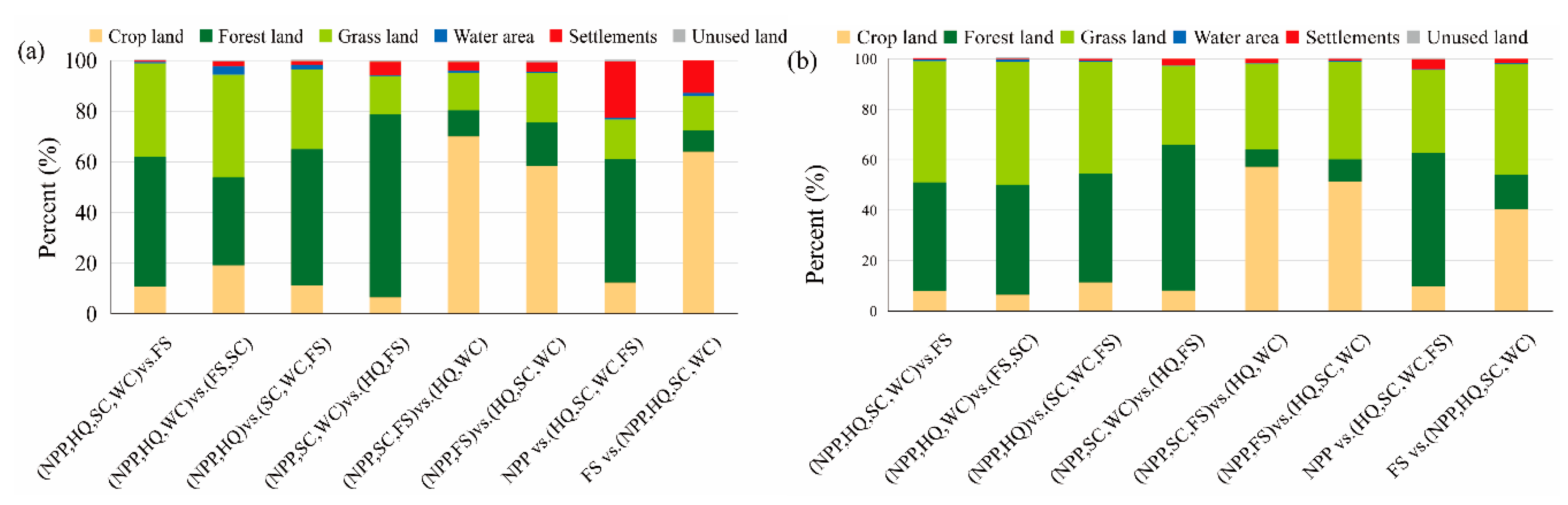
3.4.2. Trade-Off Relationships in Various Land Use Types

The interactions among multiple ESs were complex based on the gird scale across two basins, so we further analyzed the patterns of trade-offs among multiple ESs in various land use types (Figure 7). In the Guanzhong Basin, the trade-offs among FS and other services (NPP, HQ, SC, and WC) (simultaneous increase) were mostly concentrated in the forest land and crop land, and occupied 51.34% and 36.90%, respectively. The trade-offs among NPP, HQ, WC (simultaneous increase, suggesting synergies), and SC, FS (simultaneous decrease) accounted for 40.44% that were located in the grass land, and 34.83% were located in the forest land. Meanwhile, the trade-offs among NPP, SC, and WC (simultaneous increase, suggesting synergies), and HQ and FS (simultaneous decrease) were mostly in the forest land, which accounted for 72.19%. it was discovered that the trade-offs among NPP and other services HQ, SC, WC, FS (simultaneous decrease) were concentrated in the forest land and settlements.
In the Hanzhong Basin, the synergies occurred among the NPP, HQ, SC, and WC (simultaneous increase), and exhibited trade-offs with FS that were aggregated in the crop land and forest land, which accounted for 48.02% and 42.98%. At the same time, the trade-offs among NPP and HQ (simultaneous increase, suggesting synergies), and SC, WC, FS (simultaneous decrease) was also concentrated in crop land and forest land. While the trade-offs among NPP, SC, FS (simultaneous increase, suggesting synergies), and WC, HQ (simultaneous decrease) accounted for 57.10% and 31.29% in crop land and grass land, respectively. It was found in the forest land and crop land that accounted for 38.72% and 57.27% where the trade-offs occurred among NPP and FS (simultaneous increase, suggesting synergies), and HQ, SC, and WC (simultaneous decrease). Furthermore, the trade-offs among FS and other services NPP, HQ, SC, and WC (simultaneous decrease) were aggregated in grass land and crop land, which accounted for 43.89% and 40.55%. Overall, the trade-off relationships were mainly concentrated on crop land and forest land in the Guanzhong Basin, while, in the Hanzhong Basin, these were aggregated in forest land and grass land.

4. Discussion

4.1. Difference Analysis of the Guanzhong and Hanzhong Basin

Because of this unique geographical location and climate environment, the land use structure and vegetation coverage exit spatial differences in the Guanzhong Basin and Hanzhong Basin, which directly generate the spatial heterogeneity of ecosystem services and the spatial correlation relationships between ecosystem services in two basins. For example, in terms of the land use structure, crop land was dominated in the Guanzhong Basin that accounted for 45.17%, and provided the provisioning services even though it has gradually decreased in recent years, which was concentrated in the central area of the basin and surrounding urban land of the bigger city. In comparison, the ecological environment is better in the Hanzhong Basin. Vegetation coverage is relatively high and the land use types were dominated by grassland and forest land, which accounted for 41.08% and 30.11%, respectively, concentrated in the edge of the basin. Consequently, the provisioning service was higher in the Guanzhong Basin and the regulating service was little bigger in the Hanzhong Basin. Furthermore, accompanying with other natural environment factors such as rainfall or spatial patterns of vegetation and different soil types, it determined the distinct temporal and spatial distribution characteristics of each ecosystem service in two basins. Under the interaction of various ecosystem services, trade-offs, and synergies presented different spatial and temporal patterns in two basins. For instance, our results showed the correlation direction between paired ES, which was the same in two basins, but the strength and change rate of trade-offs and synergies was strong in the Guanzhong Basin than that in the Hanzhong Basin. As the rapid economic development and the expansion of construction land, ecosystem services have suffered a down trend in the Guanzhong Basin over the past years. Meanwhile, it increased the conflict of human demand for the ecosystem. At the same time, results showed the strong trade-offs were discovered in the central region of the Guanzhong Basin, particularly in the edge of Xi’an City as the capital of Shaanxi Province. The construction land was expended with the population growth. The demand of supply services gradually increased, while the value of regulating services continued to decline, so it became the higher decreasing areas of ecosystem services, which caused the strong trade-offs [42]. Furthermore, the regulating services were mostly provided by forest land, grassland, and water areas. The trade-off relationships became strong since these areas decreased. For example, in the southeast region of the Hanzhong Basin, the conversion of grassland to cropland lead to strong trade-offs between FS and SC. Therefore, the local government should formulate the corresponding target and ecological restoration approach, according to the regional ecological demand and social development, in order to realize the sustainable supply of ecosystem services [24,43].

4.2. Temporal and Spatial Changes of Trade-Offs and Synergies

Our results showed the synergies between NPP, habitat quality, soil conservation, and water conservation that existed in two basins. This result agrees with other published findings [18,33,41]. Nevertheless, when the trade-off or synergy is weak in a region, it could be easily changed from trade-offs to synergies or inverse under the influence of local policy and planning [20]. Since 2001, the government has implemented the Reforestation of Cultivated Land project in the Shaanxi Province. Some deep slope of crop land is converted into forest land or grassland. Consequently, services provide by crop land were reduced, whereas water conservation services by grassland were greatly improved. It was discovered that relationships between NPP and WC as well as SC and WC were changed into negative relationships in 2010 in two basins because, compared with 2005, the increased rate of WC was much higher than that of SC, while NPP showed a decreasing trend. Although its crop land has decreased, demand for food supply in the urban area was enhanced, and it could enhance the giving services in grassland and water areas. Consequently, the conflict relationship between FS and WC was reduced, even when presented with a synergic relationship in the Guanzhong Basin in 2010. Therefore, the research found the trade-offs and synergies between ESs have temporal variations under the influence of different land use structures, environment factors, and social development demand (e.g., urban expansion) [44].
In addition, the landscape structure determines the ability of the ecosystem to provide the service, which humans ultimately depend on [45]. Ecosystem service relationships are affected by land use conflict [46,47]. Furthermore, spatial correlation analysis illustrates the differences of spatial distribution of two ecosystem services for a given year, ignoring the prerequisites of dynamic changes of ecosystem services and true interaction when considering the trade-offs and synergies [25]. Therefore, based on the correlation coefficients of two time series on the gird scale, we could further explore the spatial distribution of trade-offs and synergies between paired ES. Among these trade-offs, those between regulating services and the food supply service have drawn more attention. For example, our results showed a negative relationship between the food supply and soil conservation based on the whole region. However, the spatial synergistic relationships between FS and SC were widely distributed in the two basins, especially in the central region of the Guanzhong Basin. This result may be interpreted as well managed and high yield farmland in the central region of the valley basin, which is beneficial for soil conservation. Both services showed an increasing trend simultaneously. On the other hand, it could be explained that the synergy disappeared, which showed a negative relationship between two services because of the data integration and land use conflict on the whole region scale. For instance, both forest land and grass land could generate the benefit of soil conservation and food supply where it may represent synergy, but their closeness to soil conservation and food supply was inconsistent. Moreover, the closeness may be changed over time [25]. Spatial scale and temporal change play the important roles in the relationship between paired ES. Meanwhile, Felipe suggested there was no single relevant scale to analyze the relationships among multiple ESs [48]. Consequently, more place-based studies with sensitivity analysis are needed for our further understanding of the spatiotemporal dynamic interactions among multiple ESs [49] in order to select the optimized spatial range for achieving the highest values of various ecosystem services.

4.3. Multiple ESs Interactions

There is no generalizable theoretical basis to ensure the balance of economic and ecology. Thus, acquiring knowledge of how multiple ESs interactions occur locally is more likely to achieve a win-win situation [50]. Contrasted with previous studies that focused on trade-offs and synergies between paired ESs [34,41], we explored the multiple ESs interactions based on the grid cells. Regarding the inherent complexity of integrated social and ecological systems, most of the ecosystem services interact with one another. A simple consideration of only ES might generate an unexpected and dramatic decline in other ESs [51]. Trade-offs often occur when provisioning service is increased as a consequence of the decrease use of other services. Nevertheless, oversupply of the services may result in the trade-offs with other services or an unsustainable eco-environment, which causes a conflict between human demand and ecological protection. Furthermore, each of the ecosystem services presented a distinct change based on the gird scales, which reflected the multiple interactions among ES. For instance, results show the trade-offs between NPP and FS (simultaneously increased, suggesting synergy) and HQ, SC, and WC (simultaneously decreased) were widespread in two basins when compared with other multiple interactions. This phenomenon indicated that, when it is transformed from grassland to forestland or from grassland to crop land, both NPP and food supply simultaneously increased and appeared as synergy. Based on the different land use change, identified the causes, and the locations of the multiple interactions among ES, which could help decision-makers develop targeted ecosystem management strategies [52].

4.4. Limitations and Future Study Directions

It is necessary to consider the influencing mechanism and future scenario predictions in a future study of ecosystem services [4]. For instance, future scenarios aim to provide a theoretical basis for the government’s ecological planning and recommendations by the simulation of ecosystem services in different land structure allocations [11]. Furthermore, the current ecological protection policy directly increases NPP, SC, and WC and some regulating services lead to the decrease of food supply services and other provisioning services, which might be unable to meet human needs. Therefore, future research aims to develop an integrated framework for simulating ESs based on the combination of land use type, climate change, government policy, and topography factors. At the same time, it could analyze the region difference and multiple ESs spatial interactions, and then select the appropriate scenario.
In this study, the ecosystem services simulation was based on a raster dataset but lacked cultural services. Under the strategic background of “One Belt and One Road” and “Guanzhong-Tianshui economic zone,” local social and economic developments have faced unprecedented opportunities. The social cultural value would play an important role in ecosystem functions, and there could also be a large uncertainty about the impact of human activities on the ecosystem process [38]. How to estimate the cultural services more reasonably, and how to simulate future ecosystem services under the influence of social-economic and eco-environment factors in particular, will be the main factors focused on in future research studies.

5. Conclusions

The Guanzhong Basin and Hanzhong Basin were selected as case study areas. Our research quantified the spatial relationship among multiple ESs (NPP, HQ, WC, SC, and FS) and explored the spatial distribution of multiple ESs interactions based on the gird scales. Results showed the direction of the correlation coefficient between paired ES was the same in two basins, but the extent of the correlation coefficient was stronger in the Guanzhong Basin than that in the Hanzhong Basin. Meanwhile, our results demonstrated the spatial trade-off relationships between paired ES were spatially aggregated in the central and the southwest of the Guanzhong Basin, and the southeast of the Hanzhong Basin. Furthermore, the multiple ES interactions were spatially heterogeneous on the gird scales across two basins. Moreover, land use change might cause the various trade-offs among multiple ES. For example, the conversion of crop land to forest land lead to NPP, HQ, SC, and WC to continuously increase and exhibited trade-offs with FS in the Guanzhong Basin. While in the Hanzhong Basin, the conversion of grassland to crop land lead to a continuous increase in NPP and FS and exhibited trade-off interactions with the three services SC, WC, and HQ. This information may help policymakers develop targeted and local ecological management measures. Furthermore, our funding could provide a theoretical basis for the sustainable development of society, economy, and ecology in Northwest China.

Author Contributions

Conceptualization, Y.S. and Z.R. Data curation, Y.D. Funding acquisition, J.L. and Z.R. Methodology, Y.S. Software, Y.S. and Y.D. Validation, J.L. and X.L. Formal analysis, Y.S. Investigation, Y.S. and X.L. Resources, Y.S. and Y.D. Writing-original draft preparation, Y.S. and J.L. Writing-review and editing, J.L., X.L., Z.R., Z.Z., and Y.D. Visualization, Y.S. Supervision, Z.R. Project administration, J.L., X.L., and Z.Z. All authors have read and agreed to the published version of the manuscript.

Funding

The National Natural Science Foundation of China (No. 41771198, 41771576 and 41801333), the Fundamental Research Funds for the Central Universities (No.GK 201901009), the NSFC - NRF Scientific Cooperation Program (Grant no. 41811540400), and the project supported by the Natural Science Basic Research Plan in Shaanxi Province of China (Program No. 2018JM4010), and China Postdoctoral Science Foundation (2019M650859 and 2019T120142) funded this research.

Acknowledgments

Acknowledgement for the meteorological data support from “National Earth System Science Data Center, National Science & Technology Infrastructure of China. (http://www.geodata.cn).” We thank the Resource and Environmental Data Cloud Platform for sharing the Land-Use/cover datasets, which could be downloaded from http://www.resdc.cn/. We are grateful to the anonymous reviewers and Jing Li (School of Geography and Tourism in Shaanxi Normal University) and Xianfeng Liu (School of Geography and Tourism in Shaanxi Normal University) for their valuable comments and suggestions that greatly improve the manuscript.

Conflicts of Interest

The authors declare no conflict of interest.

Appendix A

In this study, multiple interactions among ESs were calculated by spatial overlay analysis based on ArcGIS. The specific calculation steps are as follows.
Step 1
We set up a set of five digit codes and make each ES correspond to one digit, respectively.
Table A1. Different digits codes for each ecosystem service.
Digits CodeTen Thousand DigitsThousand DigitsHundred DigitsTen DigitsSingle Digits
ESNPPHQSCWCFS
Step 2
We made the subtraction operations on each ES in 2000 and 2018 by the ArcGIS raster calculation, and reclassified the difference value 1, 2, and 3 to increased, reduced, and no change pixel, respectively.
2018 NPP2010 NPP
23159131710
202417152019
2862122612
1413117158
2018 NPP–2010NPPreclassify
NPP_Reclassified
10−2−110,00020,00020,000
54−210,00010,00020,000
60910,00030,00010,000
7−2310,00020,00010,000
Step 3
We performed spatial overlay operations for the reclassified layers, and recognized the interactions among multiple ecosystem services by interpreting the codes in the pixels of the output layers of overlay analysis.
NPP_ReclassifiedHQ_ReclassifiedSC_Reclassified
10,00020,00020,000020000300002000002000020000200
10,00010,00020,000010000200002000002000020000100
10,00030,00010,000020000200002000001000020000200
10,00020,00010,000020000200001000002000010000100
WC_ReclassifiedFS_Reclassified
000100002000020000020000100001
000200002000020000010000200001
000200001000020000020000100001
000100001000010000010000100002
Spatial Overlay
ES_Layer_Overlaid
12,21223,22122,221
11,22112,22222,121
12,12232,21112,221
12,21122,11111,112
The results of the table indicates the locations where multiple interactions among ecosystem services occurred based on the gird cell. For example: the code 12212” indicates that NPP, WC increased simultaneously (suggesting synergies), HQ, SC, FS decreased simultaneously, and the two services NPP, WC both exhibited trade-offs with the three services HQ, SC, and FS.

References

  1. Costanza, R.; De Groot, R.; Farber, S.; Grasso, M.; Hanno, B.; Karin, L. The value of the world’ s ecosystem services and natural capital. Nature 1997, 25, 3–15. [Google Scholar]
  2. Liu, J.; Li, J.; Qin, K.; Zhou, Z.; Yang, X.; Li, T. Changes in land-uses and ecosystem services under multi-scenarios simulation. Sci. Total Environ. 2017, 586, 522–526. [Google Scholar] [CrossRef] [PubMed]
  3. Costanza, R.; De Groot, R.; Braat, L.; Kubiszewski, I.; Fioramonti, L.; Sutton, P.; Grasso, M. Twenty years of ecosystem services: How far have we come and how far do we still need to go? Ecosyst. Serv. 2017, 28, 1–16. [Google Scholar] [CrossRef]
  4. Li, B.; Chen, N.; Wang, Y.; Wang, W. Spatio-temporal quantification of the trade-offs and synergies among ecosystem services based on grid-cells: A case study of Guanzhong Basin, NW China. Ecol. Indic. 2018, 94, 246–253. [Google Scholar] [CrossRef]
  5. Li, S.; Zhang, C.; Liu, J.; Zhu, W.; Ma, C.; Wang, Y. The tradeoffs and synergies of ecosystem services: Research progress, development trend, and themes of geography. Geogr. Res. 2013, 32, 1379–1390. [Google Scholar]
  6. Briner, S.; Huber, R.; Bebi, P.; Elkin, C.; Schmatz, D.R.; Grêt-Regamey, A. Trade-offs between ecosystem services in a mountain region. Ecol. Soc. 2013, 18, 35. [Google Scholar] [CrossRef] [Green Version]
  7. Bennett, E.M.; Peterson, G.D.; Gordon, L.J. Understanding relationships among multiple ecosystem services. Ecol. Let. 2009, 12, 1394–1404. [Google Scholar] [CrossRef]
  8. Turkelboom, F.; Thoonen, M.; Jacobs, S.; García-Llorente, M.; Martín-López, B.; Berry, P. Ecosystem services trade-offs and synergies (draft). Available online: www.openness-project.eu/library/reference-book (accessed on 16 January 2016).
  9. Tilman, D.; Cassman, K.G.; Matson, P.A.; Naylor, R..; Polasky, S. Agricultural sustainability and intensive production practices. Nature 2002, 418, 671–677. [Google Scholar] [CrossRef]
  10. Han, Z.; Song, W.; Deng, X.; Xu, X. Trade-Offs and Synergies in Ecosystem service within the Three-Rivers Headwater Region, China. Water 2017, 9, 588. [Google Scholar] [CrossRef] [Green Version]
  11. Fu, Q.; Hou, Y.; Wang, B.; Bi, X.; Li, B.; Zhang, X. Scenario analysis of ecosystem service changes and interactions in a mountain-oasis-desert system: A case study in Altay Prefecture, China. Sci. Rep. UK 2018, 8, 12939. [Google Scholar] [CrossRef] [PubMed]
  12. Torralba, M.; Fagerholm, N.; Hartel, T.; Moreno, G.; Plieninger, T. A social-ecological analysis of ecosystem services supply and trade-offs in European wood-pastures. Sci. Adv. 2018, 4, 2176. [Google Scholar] [CrossRef] [PubMed] [Green Version]
  13. Ament, J.M.; Moore, C.A.; Herbst, M.; Cumming, G.S. Cultural ecosystem services in protected areas: Understanding bundles, trade-offs, and synergies. Conserv. Lett. 2017, 10, 440–450. [Google Scholar] [CrossRef]
  14. Cord, A.F.; Bartkowski, B.; Beckmann, M.; Dittrich, A.; Hermans-Neumann, K.; Kaim, A.; Lienhoop, N.; Locher-Krause, K.; Priess, J.; Schröter-Schlaack, C.; et al. Towards systematic analyses of ecosystem service trade-offs and synergies: Main concepts, methods and the road ahead. Ecosyst. Serv. 2017, 28, 264–272. [Google Scholar] [CrossRef]
  15. Bai, Y.; Zhuang, C.; Ouyang, Z.; Zheng, H.; Jiang, B. Spatial characteristics between biodiversity and ecosystem services in a human-dominated watershed. Ecol. Complex. 2011, 8, 177–183. [Google Scholar] [CrossRef]
  16. Howe, C.; Suich, H.; Vira, B.; Mace, G.M. Creating win-wins from trade-offs? Ecosystem services for human well-being: A meta-analysis of ecosystem service trade-offs and synergies in the real world. Glob. Environ. Chang. 2014, 28, 263–275. [Google Scholar] [CrossRef] [Green Version]
  17. Plieninger, T.; Torralba, M.; Hartel, T.; Fagerholm, N. Perceived ecosystem services synergies, trade-offs, and bundles in European high nature value farming landscapes. Landscape Ecol. 2019, 34, 1565–1581. [Google Scholar] [CrossRef]
  18. Raudsepp-Hearne, C.; Peterson, G.D.; Bennett, E.M. Ecosystem service bundles for analyzing tradeoffs in diverse landscapes. Proc. Natl. Acad. Sci. USA 2010, 107, 5242–5247. [Google Scholar] [CrossRef] [Green Version]
  19. Demestihas, C.; Plénet, D.; Génard, M.; Raynal, C.; Lescourret, F. A simulation study of synergies and tradeoffs between multiple ecosystem services in apple orchards. J. Environ. Manag. 2019, 236, 1–16. [Google Scholar] [CrossRef]
  20. Wang, Y.; Li, X.; Zhang, Q.; Li, J.; Zhou, X. Projections of future land use changes: Multiple scenarios-based impacts analysis on ecosystem services for Wuhan city, China. Ecol. Indic. 2018, 94, 430–445. [Google Scholar] [CrossRef]
  21. Grasso, M. Ecological–economic model for optimal mangrove trade-off between forestry and fishery production: Comparing a dynamic optimization and a simulation model. Ecol. Model. 1998, 112, 131–150. [Google Scholar] [CrossRef]
  22. Seppelt, R.; Lautenbach, S.; Volk, M. Identifying trade-offs between ecosystem services, land use, and biodiversity: A plea for combining scenario analysis and optimization on different spatial scales Ralf Seppelt1, Sven Lautenbach2 and Martin Volk1. Curr. Opin. Env. Sust. 2013, 5, 458–463. [Google Scholar] [CrossRef]
  23. Bohensky, E.L.; Reyers, B.; Jarrsveld, A.S.V. Conservation in practice: Future ecosystem services in a Southern African River Basin: A scenario planning approach to uncertainty. Conserv. Biol. 2006, 20, 1051–1061. [Google Scholar] [CrossRef] [PubMed]
  24. Gong, J.; Liu, D.; Zhang, J.; Xie, Y.; Cao, E.; Li, H. Tradeoffs/synergies of multiple ecosystem services based on land use simulation in a mountain-basin area, western China. Ecol. Indic. 2019, 99, 283–293. [Google Scholar] [CrossRef]
  25. Zheng, Z.; Fu, B.; Hu, H.; Sun, G. A method to identify the variable ecosystem services relationship across time: A case study on Yanhe Basin, China. Landscape Ecol. 2014, 29, 1689–1696. [Google Scholar] [CrossRef] [Green Version]
  26. Zhang, Y.M.; Li, J.; Zeng, L.; Yang, X.; Liu, J.; Zhou, Z. Optimal protected area selection: Based on multiple attribute decision making method and ecosystem service research—Illustrated by Guanzhong-Tianshui Economic Region section of the Weihe River Basin. Sci. Agric. Sin. 2019, 52, 2114–2127. [Google Scholar]
  27. Peng, J.; Hu, X.; Wang, X.; Meersmans, J.; Liu, Y.; Qiu, S. Simulating the impact of Grain-for-Green Programme on ecosystem services trade-offs in Northwestern Yunnan, China. Ecosyst. Serv. 2019, 39, 100998. [Google Scholar] [CrossRef]
  28. Qin, K.; Li, J.; Liu, J.; Yan, L.; Huang, H. Setting conservation priorities based on ecosystem services - A case study of the Guanzhong-Tianshui Economic Region. Sci. Total Environ. 2019, 650, 3062–3074. [Google Scholar] [CrossRef]
  29. Hadian, F.; Jafari, R.; Bashari, H.; Tartesh, M.; Clarke, K.D. Estimation of spatial and temporal changes in net primary production based on Carnegie Ames Stanford Approach (CASA) model in semi-arid rangelands of Semirom County, Iran. J. Arid Land. 2019, 11, 477–494. [Google Scholar] [CrossRef] [Green Version]
  30. Potter, C.S.; Randerson, J.T.; Field, C.B.; Matson, P.A.; Vitousek, P.M.; Mooney, H.A.; Klooster, S.A. Terrestrial ecosystem production: A process model based on global satellite and surface data. Global Biogeochem Cy. 1993, 7, 811–841. [Google Scholar] [CrossRef]
  31. Loreau, M.; Naeem, S.; Inchausti, P.; Bengtsson, J.; Grime, J.P.; Hector, A.; Hooper, D.U.; Huston, M.A.; Raffaelli, D.; Schmid, B.; et al. Biodiversity and ecosystem functioning: Current knowledge and future challenges. Science 2001, 294, 804–808. [Google Scholar] [CrossRef] [Green Version]
  32. Hector, A.; Bagchi, R. Biodiversity and ecosystem multifunctionality. Nature 2007, 448, 188–190. [Google Scholar] [CrossRef] [PubMed]
  33. Hou, Y.; Lü, Y.; Chen, W.; Fu, B. Temporal variation and spatial scale dependency of ecosystem service interactions: A case study on the central Loess Plateau of China. Landscape Ecol. 2017, 32, 1201–1217. [Google Scholar] [CrossRef]
  34. Asadolahi, Z.; Salmanmahiny, A.; Sakieh, Y.; Mirkarimi, S.H.; Baral, H.; Azimi, M. Dynamic trade-off analysis of multiple ecosystem services under land use change scenarios: Towards putting ecosystem services into planning in Iran. Ecol. Complex. 2018, 36, 250–260. [Google Scholar] [CrossRef]
  35. Bao, Y.; Liu, K.; Li, T. Effects of land use change on habitat based on InVEST model: Taking yellow river wetland nature reserve in Shaanxi province as an example. Arid Zone Res. 2015, 32, 622–629. [Google Scholar]
  36. Biao, Z.; Wenhua, L.; Gaodi, X.; Yu, X. Water conservation of forest ecosystem in Beijing and its value. Ecol. Econ. 2010, 69, 1416–1426. [Google Scholar] [CrossRef]
  37. Li, J.; Ren, Z. Spatiotemporal change of water conservation value of Loess Plateau ecosystem in northern Shaanxi Province. Chin. J. Ecol. 2008, 27, 240–244. [Google Scholar]
  38. Shi, Z.H.; Cai, C.F.; Ding, S.W.; Wang, T.W.; Chow, T.L. Soil conservation planning at the small watershed level using RUSLE with GIS: A case study in the Three Gorge Area of China. CATENA 2004, 55, 33–48. [Google Scholar] [CrossRef]
  39. Liu, B.Y.; Nearing, M.A.; Shi, P.J.; Jia, Z.W. Slope length effects on soil loss for steep slopes. Soil Sci. Soc. Am. J. 2000, 64, 1759. [Google Scholar] [CrossRef] [Green Version]
  40. Yang, X.; Zhou, Z.; Li, J.; Fu, X.; Mu, X.; Li, T. Trade-offs between carbon sequestration, soil retention and water yield in the Guanzhong-Tianshui Economic Region of China. J. Geogr. Sci. 2016, 26, 1449–1462. [Google Scholar] [CrossRef]
  41. Power, A.G. Ecosystem services and agriculture: Tradeoffs and synergies. Philos. Trans. R. Soc. B Biol. Sci. 2010, 365, 2959–2971. [Google Scholar] [CrossRef]
  42. Sun, Y.; Ren, Z.; Zhao, S.; Zhang, J. Spatial and temporal changing analysis of synergy and trade-off between ecosystem services in valley basins of Shaanxi Province. Acta Geogr. Sin. 2017, 72, 521–532. [Google Scholar]
  43. Zhu, Y.; Zhongke, F.; Lu, J.; Liu, J. Estimation of forest biomass in Beijing (China) using multisource remote sensing and forest inventory data. Forest 2020, 11, 163. [Google Scholar] [CrossRef] [Green Version]
  44. Qiao, X.; Gu, Y.; Zou, C.; Xu, D.; Wang, L.; Ye, X.; Yang, Y.; Huang, X. Temporal variation and spatial scale dependency of the trade-offs and synergies among multiple ecosystem services in the Taihu Lake Basin of China. Sci. Total Environ. 2019, 651, 218–229. [Google Scholar] [CrossRef] [PubMed]
  45. Fan, M.; Xiao, Y. Impacts of the grain for Green Program on the spatial pattern of land uses and ecosystem services in mountainous settlements in southwest China. Glob. Ecol. Conserv. 2020, 21, e806. [Google Scholar] [CrossRef]
  46. Xu, S.; Liu, Y.; Wang, X.; Zhang, G. Scale effect on spatial patterns of ecosystem services and associations among them in semi-arid area: A case study in Ningxia Hui Autonomous Region, China. Sci. Total Environ. 2017, 598, 297–306. [Google Scholar] [CrossRef]
  47. Li, S.; Bing, Z.; Jin, G. Spatially explicit mapping of soil conservation service in monetary units due to land use/cover change for the Three Gorges Reservoir Area, China. Remote Sens. (Basel) 2019, 11, 468. [Google Scholar] [CrossRef] [Green Version]
  48. Felipe-Lucia, M.R.; Comín, F.A.; Bennett, E.M. Interactions among ecosystem services across land uses in a floodplain agroecosystem. Ecol. Soc. 2014, 19, 20. [Google Scholar] [CrossRef] [Green Version]
  49. Yi, H.; Güneralp, B.; Kreuter, U.P.; Güneralp, İ.; Filippi, A.M. Spatial and temporal changes in biodiversity and ecosystem services in the San Antonio River Basin, Texas, from 1984 to 2010. Sci. Total Environ. 2018, 619–620, 1259–1271. [Google Scholar] [CrossRef]
  50. Li, T.; Lü, Y.; Fu, B.; Hu, W.; Comber, A.J. Bundling ecosystem services for detecting their interactions driven by large-scale vegetation restoration: Enhanced services while depressed synergies. Ecol. Indic. 2019, 99, 332–342. [Google Scholar] [CrossRef] [Green Version]
  51. Fu, Q.; Li, B.; Hou, Y.; Bi, X.; Zhang, X. Effects of land use and climate change on ecosystem services in Central Asia’s arid regions: A case study in Altay Prefecture, China. Sci. Total Environ. 2017, 607–608, 633–646. [Google Scholar] [CrossRef]
  52. Aurenhammer, P.K. Nudging in the Forests—the Role and Effectiveness of NEPIs in Government Forest Initiatives of Bavaria. Forests 2020, 11, 168. [Google Scholar] [CrossRef] [Green Version]
Figure 1. The geographical location and land use types of study areas in 2018.
Forests 11 00209 g001
Figure 2. The spatial distribution of average ecosystem services in valley basins from 2000 to 2018.
Forests 11 00209 g002
Figure 3. The relationships between average ecosystem services in the Guanzhong Basin (A) and in the Hanzhong Basin (B) from 2000 to 2018. Based on the R software, pie chart, and scatter plot can directly indicate the relationships between ecosystem services. For example, in the pie chart, the blue color represented positive values, the red color represented negative values, and the intensity of the color increased uniformly as the correlation value increased. The shading of the lower triangular in the figure had the same meanings in color as the circles of the upper triangular. Furthermore, the intensity of color scaled in proportion to the magnitude of correlation values, besides the circles were filled clockwise for positive values and anti-clockwise for negative values. In the scatter plot, all data may be considerably enhanced by the addition of linear regression lines, (loess) smoothed curves, and so forth. The key diagonal represented the kernel density curve and the lower horizontal axis was the shaft figure. Other figures contained linear and smooth fitting curves.
Forests 11 00209 g003
Figure 4. Spatial correlation coefficient for each pair of ecosystem services in two basins from 2000 to 2018.
Forests 11 00209 g004
Figure 5. Spatial trade-offs and synergies of paired ecosystem services in two valley basins. ** Correlation were all significant at the 0.01 level. * Correlation were all significant at the 0.05 level. (a,b): Spatial trade-offs and synergies for HQ (habitat quality) and NPP (net primary production) in Guanzhong and Hanzhong Basin, respectively. (c,d): Spatial trade-offs and synergies for WC (water conservation) and NPP. (e,f): Spatial trade-offs and synergies for FS (food supply) and HQ. (g,h): Spatial trade-offs and synergies for FS and SC (soil conservation).
Forests 11 00209 g005
Figure 6. The spatial patterns of multiple interactions among ecosystem services (ESs) in two basins from 2000 to 2018. Because the ecosystem service assessments were based on the gird scales, the interactions among multiple ESs were complex. Some bigger area proportions and clear interactions were shown in the figure, and others are collectively named “other interactions”; ‘+’ indicated an increase of service; ‘−’ indicated a reduction. For example, “NPP+, HQ+, SC−, WC−, FS−” indicates that NPP (net primary production), HQ (habitat quality) increase simultaneously (suggesting synergies), SC (soil conservation), WC (water conservation), FS (food supply) decrease simultaneously, and the two services NPP, HQ both exhibit trade-off relationships with other three services WC, SC, FS. Moreover, We selected four evident trade-offs location (AD) where the areas were 1km2, and further amplified and analyzed these interactions.
Forests 11 00209 g006
Figure 7. Trade-offs and synergies among multiple ecosystem services in different land use types.
Forests 11 00209 g007

