Optimizing Forest Spatial Structure with Neighborhood-Based Indices: Four Case Studies from Northeast China

Abstract

The fine-scale spatial patterns of trees and their interactions are of paramount importance for controlling the structure and function of forest ecosystems; however, few management techniques can be employed to adjust the structural characteristics of uneven-aged mixed forests. This research provides an accurate, efficient, and impersonal comprehensive thinning index (P-index) for selecting candidate harvesting trees; the index was proposed by weighting the commonly used quantitative indices with respect to stand fine-scale structures, competition status, tree vigor, and tree stability. The applications of the proposed P-index in evaluating and simulating the process of thinning operations were examined using four 1-ha mapped plots with different forest types, namely, natural secondary forest, natural pine-broadleaved mixed forest, natural larch-birch mixed forest, and natural oak forest, which were widely distributed across the Heilongjiang Province in Northeast China. The results indicated that the proposed P-index could effectively affect the structural differentiations between different forest types and alternative thinning intensities. The marginal benefits of alternative thinning intensities on the integrated forest structure indicated that removing 10% of the trees from the plots might be the optimal thinning intensity from the perspective of optimizing stand structure, in which the P-index values could be increased by approximately 5%–11% for the four tested plots. The main conclusion from this paper was that the proposed P-index could be used as a quantitative tool to manage uneven-aged mixed forests.

1. Introduction

Forest structure, including spatial and nonspatial characteristics, is one attribute contributing to the sustainable management of mixed uneven-aged forests. The nonspatial forest structure usually describes the average states of forest attributes, such as the mean diameter at breast height (DBH), mean tree height (HT), and stand density, which have been widely used in forest resource surveys, management, and monitoring [1]. Spatial forest structures exist at a variety of spatial scales and are of paramount importance for determining habitat and species diversity, which can be roughly divided into four levels: alpha, beta, gamma, and delta [2,3]. In forest ecosystems, the gamma and delta levels usually operate on landscape scales or at large forest areas, reflecting the fragmentation degrees of habitat and landscape; in contrast, the beta level refers to the variation between forest stands, reflecting the substitutability degree of different species under habitat gradients (e.g., elevation and succession stage), and the alpha level usually operates within forest stands, mainly reflecting the species richness, relative abundance, and uniformity. Many studies have been carried out at landscape levels and especially at stand levels [4,5], mainly due to the availability of advanced techniques (e.g., remote sensing) used to sample at the landscape (or regional) scale and the accessibility of data collection at the forest stand scale. However, there is an increasing demand for information on the alpha scale, particularly regarding the fine-scale spatial distribution of trees and their attributes [3,6,7], as societal values have changed from focusing on traditional timber to the diversified benefits and multiple functions of forest ecosystems in recent decades.

In recent decades, several methods and indices have been widely developed to describe forest structural attributes. From the perspective of mathematical terms, most of these indices can be divided into two major groups: distance-independent measures and distance-dependent measures [3]. The first group evaluates stand structure without any spatial reference (e.g., Shannon index), while spatial references are necessary for the latter group, and they can be further subdivided into (1) individual tree parameters based on neighborhood relations at a fine scale, such as species mingling and contagion index [3,7]; (2) distance-dependent measures to describe the forest stand structure at the stand level, such as Clark and Evans’s segregation index [8] and Pielou’s segregation index [9]; and (3) continuous functions to describe the forest structure by considering all possible inter-tree distances, such as Ripley’s K function [10] and Weigand’s O-ring function [11]. However, the distance-dependent indices can provide only the average status of the structure of a particular forest and cannot be used to describe the great variety of spatial arrangements, especially in very complex and mixed uneven-aged forests where the fine-scale structural characteristics are highly variable. The continuous functions are useful for describing forest structures, but they require datasets with known tree positions, of which the applicable data collection processes are very time consuming and expensive. For these reasons, the use of neighborhood-based parameters for describing forest structural information at fine scales has drawn much attention since the 1990s. According to Pommerening [3], the stand structure at smaller scales can be defined as the diversity of tree positions (spatial distribution), the diversity of tree species, and the diversity of tree dimensions, which highly depend on the spatial relationships of neighborhood trees. There are, of course, a considerable number of indices used to describe forest spatial structure (see details in [3]); however, the uniform angle index (U), the species mingling index (M), and the diameter dominance index (D) are the most attractive indicators for describing the three main aspects of trees in a forest stand [3,7,12,13,14,15]. Since the stand spatial structures have significant effects on both biotic and abiotic values as well as on the abundance of flora and fauna species, assessing and understanding the spatial structure characteristics has become an important foundation for implementing sustainable forest management.

Forest thinning is a typical and important management treatment that can improve forest growth, stand structure, and timber value; provide a suite of forest ecosystem services [16,17,18]; and influence the understory microclimates, soil water content, nutrient cycles, and natural hazards (e.g., forest fires, plant diseases, and insect pests) [19,20,21]; however, unreasonable thinning may sometimes result in counterproductive outcomes, such as damaging the understory, inhibiting seed germination, and even reducing tree species diversity. Therefore, how to scientifically select trees as candidates for logging is the key question for thinning, in practice. Since the thinning process is usually irreversible and difficult to repeat, the process of selection for harvest should be quite prudent and restricted by a number of factors. Traditional forest management models usually aim to improve forest growth and timber yield by adjusting the stand-level characteristics and population structure, such as the age structure, DBH distribution, species composition, and stand density; however, these models may be not available for uneven-aged and mixed forests, mainly because the potential demands of the diversity of forest structures are ignored. In recent decades, several thinning methods have been proposed and widely implemented for uneven-aged forest management practices, including the comprehensive indices approach [22], the stem number guide curve [23], and target tree-oriented management [24]; however, these approaches have mainly focused on stem size and stem form and have lacked any relevant information with respect to their spatial structure. Recently, a comprehensive index approach based on some frequently used stand spatial structure indices (e.g., U-, M-, and D-indices) has been developed to evaluate stand spatial structure characteristics according to the structure-based forest management (SBFM) strategy [7,25]; however, the applicability of these comprehensive indices to optimizing forest spatial structure has not been widely evaluated. The study by Li et al. [26] is an example that has utilized a comprehensive index for selecting candidate trees for harvest according to the bivariate distributions of the three spatial parameters (i.e., U-, M-, and D-indices). However, the nonspatial indices of individual trees were all severely absent within the above studies. In fact, stand spatial and nonspatial attributes are almost equally important in controlling the timber values and the function of forest ecosystem services. Therefore, integrating spatial and nonspatial stand indicators together into the process of optimizing forest spatial structure may be more practical from the perspective of forest management.

The purpose of our study was to put forward a comprehensive thinning index based on tree neighborhood-based spatial relationships and nonspatial individual growth status. The comprehensive index was then employed to implement parametric thinning simulations for four different forest types across the province of Heilongjiang in Northeast China. Our hypotheses were as follows: (1) the proposed comprehensive thinning index can reflect the structural differentiations between different forest types, (2) the SBFM strategy can improve the complexity and diversity of stand spatial structures at fine scales, and (3) there is an optimal thinning intensity that can effectively improve the stand spatial structure characteristics.

2. Materials and Methods

2.1. Case Study Areas

Our test stands included four different forest types across the entire Heilongjiang Province in Northeast China (Figure 1), which are the major forest types in Northeast China [27]. The first stand is a mixed larch-birch (Larix gmelinii (Ruprecht) Kuzeneva-Betula platyphylla Suk.) deciduous forest (Plot a) located in the Cuigang Forest Farm (123°20′–124°21′E, 52°16′–52°47′N), which is part of the Daxing’an Mountains [28]. The terrain in this area is of mainly low- to medium-elevation mountains that trend significantly from northeast to southwest, with many valleys and overlapping peaks. The elevation of this region varies between 180 and 1530 m a.s.l., and the average elevation is approximately 573 m. The climate belongs to a cold-temperate continental monsoon climate with typical short, warm, humid summers and long, cool, dry winters. The average annual temperature is −2.8 °C, with a maximum temperature of 40.6 °C and a minimum temperature of −52.3 °C. The average annual precipitation ranges between 450 and 500 mm, and precipitation occurs primarily in the summer. The periods of snow cover in forests are as long as five months, and the thickness of snow is close to 50 cm. The soils are classified as dark brown coniferous forest soils that are formed under the combined influences of heat and moisture in mixed forests; however, meadow and swamp soils are also common in regions with low elevations. Natural L. gmelinii forests are historically the primary top zonal vegetation; however, most have disappeared, since excessive cutting was carried out between 1950 and 2000. Large trees were frequently removed from the forests for structural timbers, leaving a mass of small and unhealthy trees. During the long period of natural succession after the cutting disturbance, some native broadleaf species have naturally regenerated in this forest community, gradually forming a mixed and uneven-aged larch-birch forest. The forest community diversities are somewhat low, mainly due to the cold temperature, and L. gmelinii, B. platyphylla, and Populus davidiana Nakai are the most common species in these mixed forests.

The second plot is a mixed Korean pine (Pinus koraiensis Siebold et Zuccarini)-broadleaved forest (Plot b) that was once the climax community of the Xiaoxing’an Mountains. The plot is located in the Danqinghe Experimental Forest Farm (129°11′–129°26′E, 46°32′–46°39′N). The reserve is a low-altitude area (190–1028 m), located approximately 45 km north of the Songhua River [16]. This area has a temperate continental monsoon climate, with a mean annual rainfall of 600 mm and a mean annual evaporation of 1250 mm. The mean annual temperature is 2 °C, and the minimum temperature is about −35 °C in the winter (January), when frozen snowfall accumulates to a depth of 20–30 cm. Dark brown forest soils also predominate across this region. The vegetation primarily consists of more than 20 tree species, classified as Xiaoxing’an Mountain flora, among which B. platyphylla and the “three great hardwoods” in Northeast China (e.g., Fraxinus mandshurica Rupr., Phellodendron amurense Rupr., and Juglans mandshurica Maxim.) predominate in valleys lower than 300 m a.s.l., while Quercus mongolica Fischer ex Ledebour and B. platyphylla gradually become more common at higher elevations (300–700 m). Abies fabri (Mast.) Craib and Picea asperata Nakai usually appear at altitudes above 700 m. The specific study site was located in the 27th compartment, which belongs to the core area of this forest farm. The study site experienced several degrees of selective cutting before 1997, followed by complete natural restoration. To optimize the structure and promote the growth of the forest, a slight under-tending treatment (e.g., removing less than 15% of smaller trees and only those with less economic value) was implemented in 2014.

The remaining two sites are the natural secondary forest (Plot c) and natural oak (Q. mongolica) forest (Plot d), located in Maoershan Forest Farm (127°18′–127°41′E, 45°2′–45°18′N), which covers an area of 26,496 ha, with a south-north length of approximately 30 km and an east-west width of 20 km [29]. It is located in a low-altitude area of the Zhangguangcai Mountains, approximately 80 km from Harbin city, the capital of Heilongjiang Province. The climate is a temperate continental monsoon climate with a mean annual temperature of 3.1 °C, a mean annual precipitation of 723 mm, a mean annual evaporation of 1094 mm, and a mean annual cumulative temperature (i.e., ≥ 10 °C) of 2283 °C. The frost-free period is approximately 120–140 days, and the relative humidity is 75%. The zonal soil is dark-brown forest soil, while azonic soils such as albic, meadow, and pear soils are common in seasonal or perennial catchment areas. The forestlands are mainly covered by natural regenerated secondary forests where the primary Korean pine-broadleaved forests have been severely damaged. Since ownership was transferred from the state to Northeast Forestry University as a trial forest farm in 1952, a large portion was subjected to complete restoration, gradually forming highly mixed natural secondary forests with more than 20 tree species. The specific study site was located in the 36th compartment for the natural secondary forest, with a slope that was shady (north-facing), downward, and gentle (13°), while the 16th compartment for the natural oak forest had a slope that was sunny (south-facing), medium, and steep (23°). To optimize species composition and promote the growth of the natural secondary forest, approximately 500 P. koraiensis trees per hectare were replanted within the forest gaps in 2004, and this was followed by complete restoration. The tree species richness is relatively higher, and F. mandshurica, P. davidiana, Ulmus pumila Linn., P. amurense, P. koraiensis, and B. platyphylla are dominant. For the natural oak forest, the study site has experienced little anthropogenic disturbance (e.g., cutting and replanting) over the last 60 years; however, the structural complexity and species richness are both lower than those of the natural secondary forest, mainly due to the significant differences between their terrains.

2.2. Plot Measurements

From June to September in 2016 and 2017, four 100 m × 100 m permanent plots were selected and estimated from the three forest farms described. To minimize the closure error of the plot area (i.e., keep it < 1/400) and the measurement errors of the positions of trees, the entire plot was divided into 100 subplots (10 m × 10 m). In each plot, the precise positions of any tree with a diameter at breast height (DBH; 1.3 m) ≥ 5 cm were recorded in three dimensions. Other tree characteristics, such as species, DBH, HT, crown width, height of living branches, and health status (e.g., survival and the presence of diseases or insects), were also recorded. The spatial distributions and basic statistical characteristics of all surveyed trees for the four plots are illustrated in

Table 1. Basic statistical characteristics of the four studied plots.

Variables	Plot a	Plot b	Plot c	Plot d
Site	Cuigang	Danqinghe	Maoershan	Maoershan
Location	52°19′13″N 123°47′23″E	46°37′36″N 129°22′22″E	45°13′21″N 127°37′40″E	45°10′37″N 127°29′9″E
Community type	Larch-birch mixed forest	Pine-broadleaved mixed forest	Natural secondary forest	Natural oak forest
Mean elevation (m)	546	399	339	407
Slope (°)	<5	<5	13	23
Slope position	Flat	Flat	Down	Medium
Slope aspect	None	None	North	South
Density (trees/ha)	2465	877	1359	1164
Mean DBH (cm)	9.59	15.27	12.53	13.48
Mean height (m)	10.94	12.75	11.84	11.2
Number of species	5	15	24	8
Disturbance type	Repeated intensive selective cutting-20 years ago	Repeated intensive selective cutting—20 years ago; slight under-tending—3 years ago	Clearcutting—60 years ago Understory replanting—15, 40 years ago	Clearcutting—60 years ago

.

2.3. Data Analysis

Reasonable forest structures, including reasonable spatial and non-spatial structural characteristics, are usually regarded as the basis for realizing sustainable forest management. Therefore, a set of ecological- and economic-oriented indicators were carefully selected to develop a composite harvesting index, which was further employed to optimize stand structure. It should be noted that all of the selected indices in this study are relative indicators (i.e., ratio indicators), which help to prevent obvious selection priority tendencies (e.g., the preferential harvesting of large or small trees and the priority harvesting of broad-leaved trees or conifers) for harvesting trees of the proposed composite thinning index.

2.3.1. Nonspatial Structural Parameters

The stand nonspatial structural characteristics were evaluated using two indices: one was related to tree vigor, and the other was related to tree stability. The tree crown is the main site for a series of important physiological activities of forests and trees, such as photosynthesis and respiration; thus, the size, structure, and distribution of the canopy can comprehensively reflect the growth vigor and development trend of trees. Previous studies have indicated that the crown size usually increases significantly with tree diameter, presenting a typical sigmoid tendency [29,30]. To eliminate the preference of tree vigor indices, the ratio of crown width with respect to DBH was employed to evaluate tree vigor:

$$V_i=\frac{C{W}_i}{DB{H}_i}=\frac{C{W}_i^e+C{W}_i^w+C{W}_i^s+C{W}_i^n}{4·DB{H}_i},$$

(1)

where V_i represents the ratio of crown width with respect to the DBH of tree i; CW_i represents the mean crown width of tree i and was calculated as the mean value of crown width in the east (CW_i ^e), west (CW_i ^w), south (CW_i ^s), and north (CW_i ⁿ) directions; and DBH_i represents the diameter at breast height of tree i. This index presents a significant exponential decay trend with increasing DBH and usually varies from 0 to 0.5 for the main tree species in Northeast China [31]. Trees with higher vigor have index values near 0.5, while trees with lower vigor have index values smaller than 0.1.

The stability of trees against snow, ice, and wind, which is known as the slenderness coefficient, was calculated by dividing the total height by the DBH of the tree [32]:

$$S_i=\frac{H{T}_i}{DB{H}_i},$$

(2)

where S_i is the height to diameter ratio of tree i, which usually has a range from 0 to 1; HT_i is the total height of tree i; and DBH_i is the diameter at breast height. The relationship between S and DBH was also a significant exponential decay function. In general, higher values of S indicate a higher position of the centre of gravity of trees with longer crown lengths, but a lower stability than trees with smaller S values [33,34]. Additionally, the S-index has significant effects on the mechanical properties of wood [35], i.e., trees with a higher S usually have a smaller maximum bending moment than do trees with a smaller S value.

2.3.2. Spatial Structural Parameters

To quantitatively determine the potential of harvesting trees from the perspective of optimizing forest spatial structural characteristics, four fine-scale spatial structural parameters were selected and employed, including the mingling index (M) [3,7,13], dominance index (D) [15], uniform angle index (U) [3,7,12], and Heygi competition index (H) [36]. In this paper, a spatial structural unit was defined as the combination of an arbitrary reference tree and its four nearest neighbor trees, as implemented in Programming [3], Li et al. [16], and Bettinger and Tang [37]. To eliminate the edge effects, a buffer area width of 5 m was employed; thus, the trees located in the core area were treated as reference trees, and the corresponding four parameters were calculated, while the other trees located in the buffer area were treated only as neighboring trees [16]. The M refers to the proportion of different species between the reference tree and its four nearest neighbors, reflecting the local-scale species diversity [13]. The D characterizes the diametric (or tree height) differentiation between a reference tree and its four nearest neighbors, which was put forward by Zhao et al. [15]. The U refers to the horizontal distribution pattern of the reference tree and its four nearest neighbors [12]. If the U values fall in the interval of 0.475–0.517, it implies a random distribution pattern [38]. Otherwise, the distribution pattern can be regular (U < 0.475) or clumped (U > 0.517). The above described parameters (i.e., M, D, and U) all include five possible values: 0.00, 0.25, 0.50, 0.75, and 1.00, which represent five different ecological grades for different aspects in the forest (

Table 2. Forest spatial structural parameters with the respective classes.

Parameter	Variable	Classes and Description
M-index∈[0, 1]	species	zero degree: M = 0.00 weak degree: M = 0.25 moderate degree: M = 0.50 strong degree: M = 0.75 extremely strong degree: M = 1.00
D-index∈[0, 1]	diameter	absolute inferior: U = 0.00 inferior: U = 0.25 homogeneous: U = 0.50 sub-superiority: U = 0.75 superiority: U = 1.00
U-index∈[0, 1]	angle	very regular: U = 0.00 regular: U = 0.25 random: U = 0.50 clumped: U = 0.75 very clumped: U = 1.00
H-index∈[0, 1]	distance and diameter	very low: H∈(0,2] low: H∈(2,4] medium: H∈(4,6] high: H∈(6,10] very high: H∈(10,+∞)

). Obviously, values close to 0 indicate a lower level of species mingling, an absolutely inferior tree growth status, and a very regular distribution pattern of trees in the horizontal dimension, while high values document high species diversity, predominant growth status, and clumped patterns. The competition index (H), which might be regarded as the modified version of Hyegi’s index [36], also refers to the competitive status, based on the properties (i.e., diameter and distance), between the reference tree and its four nearest neighbors. This index is a continuous variable, and the values may theoretically range from 0 to +∞. The formulations of the four spatial structural indices are stated as:

$$M_{\mathrm{i}}=\frac{1}{n}{\displaystyle \sum _{i=1}^n{v}_{ij},}{v}_{ij}=\{\begin{array}{l}1\mathrm{if}s{p}_j\ne s{p}_i\\ 0\mathrm{if}s{p}_j=s{p}_i\end{array},$$

(3)

$$D_{\mathrm{i}}=\frac{1}{n}{\displaystyle \sum _{i=1}^n{k}_{ij},}{k}_{ij}=\{\begin{array}{l}1\mathrm{if}db{h}_j<db{h}_i\\ 0\mathrm{if}db{h}_j\ge db{h}_i\end{array},$$

(4)

$$U_{\mathrm{i}}=\frac{1}{n}{\displaystyle \sum _{i=1}^n{z}_{ij},}{z}_{ij}=\{\begin{array}{l}1\mathrm{if}{\alpha }_j<{\alpha }_0\\ 0\mathrm{if}{\alpha }_j\ge {\alpha }_0\end{array},$$

(5)

$$H_{\mathrm{i}}=\frac{1}{n}{\displaystyle \sum _{i=1}^n\frac{db{h}_i}{db{h}_j\cdot L_{ij}}},$$

(6)

where M_i, D_i, U_i, and H_i represent the mingling degree, diametric differentiation, spatial pattern, and competition pressure for reference tree i, respectively; n is the number of neighbor trees for any reference tree; and v_ij, k_ij, and z_ij are discreteness variables and are set as different values according to the following criteria: (1) v_ij = 1, if reference tree i and its neighbor tree j are of different tree species, otherwise, v_ij = 0; (2) k_ij=1, if neighbor tree j is smaller than the reference tree i, otherwise, v_ij = 0; and (3) z_ij = 1, if the angle α of two neighbor trees (e.g., the angle of neighbor trees j and j-1) is smaller than the expected standard angle α₀ (α₀ = 72°) [39], or otherwise z_ij = 0. sp_i and sp_j represent the tree species of reference tree i and its neighbor tree j, respectively; dbh_i and dbh_j represent the diameter at breast height of reference tree i and its neighbor tree j, respectively; and L_ij represents the Euclidean distance between reference tree i and its neighbor tree j. Details about the essential characteristics and classification criteria of these parameters are illustrated in Table 2.

2.3.3. Comprehensive Thinning Index

The quantitative spatial and non-spatial indices described above all have clear biological significance and can be rapidly assessed in the field, making the selection of candidate trees possible by evaluating the relationship between each reference tree and its four nearest neighbors. Since the magnitudes and measuring units of these indices are all markedly different, the comprehensive thinning index was formulated in utility theoretic as follows [40]:

$$P_{\mathrm{i}}={\displaystyle \sum _{k=1}^N{w}_k{f}_k(x_{ik})},$$

(7)

where P_i is the comprehensive thinning index of tree i, N is the number of selected quantitative indices of tree growth status and spatial structural characteristics, w_k and f_k() are the relative importance (or weight) and sub-utility function of the k-th index, respectively, and x_ik is the quantity of the k-th index for tree i. Obviously, smaller values of P for any reference tree indicate a higher probability of the tree being harvested.

As emphasized here, the relative importance of objectives (w_k() in Equation (7)) should be considered carefully as a part of the comprehensive harvesting index design; however, little guidance can be drawn from the literature about how to assign the weights of each index in SBFM. Therefore, two different weighting coefficient schemes were employed for testing purposes. The first scheme assumed that all objectives had equal importance, i.e., that all w_k values in Equation (7) were 0.1667 (precisely 1/6). However, the weights of all considered indices within the second scheme were assumed to be 0.10 for the dominance index; 0.15 for tree vigor, tree stability, and uniform angle index; 0.20 for the mingling index; and 0.25 for competition pressure. In addition, the intensity of selective cutting is also an inherent part of any forest harvest scheduling model; thus, the effects of four different levels of selective cutting intensity (i.e., removing 10%, 20%, 30%, or 40% of the trees) on the stand spatial structural characteristics were quantitatively evaluated. The intensities of 20% and 30% reflect the present situation of forest management practices in Northeast China [41,42], while the intensities of 10% and 40% are somewhat under- or over-estimated, respectively, compared to the actual ranges.

The sub-utility functions (f_k() in Equation (7)) for tree vigor (V), mingling index (M), and dominance index (D) increased linearly, so that a quantity (x_ik in Equation (7)) equal to zero gave a sub-utility of zero, while the maximum possible quantity of the goal variable produced a sub-utility of one (Figure 2a). For tree stability (S) and competition pressure (H), a linear decreasing function was employed, in which the maximum possible quantity of each index corresponded to a sub-utility of 1.0, and the minimum possible quantity produced a sub-utility of zero (Figure 2b). The sub-utility of the uniform angle index (U) increased linearly from zero to one when the quantity increased from zero to 0.5 and then decreased to zero when the quantity further increased to one (Figure 2c). As emphasized here, the minimum, mean, and maximum values were calculated for each plot separately.

3. Results

The statistical characteristics of different spatial parameters for the four forest types with alternative selective thinning intensities (i.e., removing 0%, 10%, 20%, 30%, and 40% of the trees) are illustrated in

Table 3. The statistical characteristics (Mean (Std)) of different optimized parameters for the four forest types with alternative selective thinning intensity, in which equal weights (i.e., 0.1667) for all indices were employed.

Plot	Intensity	Number /Trees 1)	DBH /cm	HT/m	D-index	U-index	M-index	S-index	V-index	H-index	P-index	RIP/% 2)
Plot a	0%	2060	9.442 (4.008)	10.535 (3.254)	0.498 (0.358)	0.565 (0.165)	0.403 (0.346)	1.183 (0.319)	0.111 (0.041)	3.588 (6.425)	0.566 (0.161)
	10%	1854	9.641 (4.020)	10.815 (2.932)	0.500 (0.355)	0.562 (0.161)	0.421 (0.343)	1.202 (0.242)	0.114 (0.037)	3.180 (2.003)	0.599 (0.101)	5.83
	20%	1648	9.960 (4.096)	10.975 (2.976)	0.503 (0.353)	0.557 (0.166)	0.468 (0.334)	1.179 (0.238)	0.114 (0.037)	2.952 (1.852)	0.611 (0.096)	2.00
	30%	1443	10.169 (4.146)	11.018 (3.006)	0.509 (0.354)	0.558 (0.164)	0.505 (0.323)	1.157 (0.234)	0.114 (0.037)	2.763 (1.751)	0.620 (0.094)	1.47
	40%	1236	10.394 (4.247)	11.086 (3.036)	0.513 (0.350)	0.553 (0.163)	0.535 (0.314)	1.138 (0.233)	0.114 (0.038)	2.566 (1.578)	0.629 (0.092)	1.45
Plot b	0%	727	15.370 (9.087)	12.546 (4.911)	0.509 (0.351)	0.578 (0.154)	0.758 (0.261)	0.913 (0.322)	0.158 (0.068)	2.577 (2.244)	0.588 (0.197)
	10%	655	16.055 (9.236)	13.247 (4.430)	0.511 (0.346)	0.572 (0.155)	0.781 (0.248)	0.940 (0.296)	0.159 (0.066)	2.449 (1.977)	0.640 (0.100)	8.84
	20%	582	16.794 (9.394)	13.503 (4.442)	0.512 (0.352)	0.562 (0.155)	0.823 (0.208)	0.908 (0.284)	0.157 (0.067)	2.247 (1.786)	0.654 (0.091)	2.19
	30%	509	17.451 (9.544)	13.703 (4.434)	0.511 (0.353)	0.554 (0.158)	0.832 (0.207)	0.879 (0.276)	0.156 (0.069)	2.059 (1.676)	0.661 (0.089)	1.07
	40%	437	18.309 (9.692)	14.026 (4.411)	0.520 (0.354)	0.556 (0.161)	0.846 (0.204)	0.852 (0.272)	0.153 (0.069)	1.864 (1.584)	0.667 (0.087)	0.91
Plot c	0%	1102	13.156 (7.317)	11.673 (5.171)	0.501 (0.363)	0.574 (0.159)	0.711 (0.262)	0.979 (0.349)	0.143 (0.072)	15.807 (49.881)	0.600 (0.205)
	10%	992	13.379 (7.343)	12.208 (4.804)	0.502 (0.362)	0.570 (0.160)	0.717 (0.261)	1.023 (0.279)	0.149 (0.065)	12.195 (39.275)	0.657 (0.096)	9.50
	20%	882	13.829 (7.515)	12.367 (4.904)	0.512 (0.358)	0.567 (0.162)	0.761 (0.235)	0.998 (0.268)	0.149 (0.065)	6.829 (22.875)	0.671 (0.086)	2.13
	30%	772	14.211 (7.697)	12.502 (5.007)	0.515 (0.354)	0.563 (0.161)	0.787 (0.228)	0.977 (0.259)	0.148 (0.066)	5.996 (19.228)	0.679 (0.082)	1.19
	40%	662	14.608 (7.783)	12.729 (5.064)	0.521 (0.352)	0.560 (0.162)	0.804 (0.222)	0.958 (0.252)	0.144 (0.064)	3.649 (12.906)	0.684 (0.080)	0.74
Plot d	0%	947	13.437 (9.007)	11.177 (3.362)	0.495 (0.350)	0.573 (0.165)	0.580 (0.305)	1.002 (0.326)	0.158 (0.086)	3.235 (3.042)	0.552 (0.209)
	10%	853	13.848 (9.172)	11.447 (3.322)	0.493 (0.350)	0.572 (0.165)	0.592 (0.304)	1.009 (0.322)	0.170 (0.078)	3.019 (2.583)	0.613 (0.104)	11.05
	20%	758	14.346 (9.490)	11.468 (3.397)	0.500 (0.347)	0.562 (0.164)	0.643 (0.270)	0.973 (0.312)	0.169 (0.080)	2.762 (2.383)	0.631 (0.092)	2.94
	30%	663	14.907 (9.841)	11.575 (3.469)	0.500 (0.349)	0.554 (0.163)	0.653 (0.268)	0.945 (0.304)	0.169 (0.083)	2.578 (2.401)	0.639 (0.088)	1.27
	40%	569	15.195 (10.072)	11.561 (3.501)	0.501 (0.352)	0.551 (0.161)	0.671 (0.266)	0.916 (0.301)	0.168 (0.086)	2.372 (2.355)	0.648 (0.084)	1.41

Note:¹⁾ The number of trees within the core area for each plot. ²⁾ The relative increased proportion of the comprehensive harvesting index (i.e., P-index in Equation (7)) between any two successive selective thinning intensities.

and

Table 4. The statistical characteristics (Mean (Std)) of different optimized parameters for the four forest types with alternative selective thinning intensity, in which unequal weights for each index were employed.

Plot	Intensity	Number /Trees 1)	DBH /cm	HT /m	D-index	U-index	M-index	S-index	V-index	H-index	P-index	RIP /% 2)
Plot a	0%	2060	9.442 (4.008)	10.535 (3.254)	0.498 (0.358)	0.565 (0.165)	0.403 (0.346)	1.183 (0.319)	0.111 (0.041)	3.588 (6.425)	0.597 (0.161)
	10%	1854	9.636 (4.023)	10.805 (2.936)	0.498 (0.356)	0.560 (0.162)	0.422 (0.342)	1.202 (0.242)	0.114 (0.037)	3.186 (2.009)	0.633 (0.092)	6.03
	20%	1648	9.886 (4.127)	10.909 (2.988)	0.500 (0.356)	0.558 (0.164)	0.479 (0.327)	1.184 (0.242)	0.114 (0.037)	2.993 (1.881)	0.647 (0.087)	2.21
	30%	1443	10.032 (4.185)	10.921 (3.017)	0.508 (0.356)	0.562 (0.164)	0.528 (0.314)	1.167 (0.241)	0.114 (0.038)	2.803 (1.780)	0.658 (0.085)	1.70
	40%	1236	10.164 (4.287)	10.899 (3.089)	0.510 (0.354)	0.561 (0.165)	0.578 (0.294)	1.148 (0.237)	0.114 (0.038)	2.649 (1.610)	0.670 (0.081)	1.82
Plot b	0%	727	15.370 (9.087)	12.546 (4.911)	0.509 (0.351)	0.578 (0.154)	0.758 (0.261)	0.913 (0.322)	0.158 (0.068)	2.577 (2.244)	0.623 (0.201)
	10%	655	16.040 (9.249)	13.233 (4.432)	0.511 (0.346)	0.573 (0.156)	0.784 (0.243)	0.941 (0.298)	0.160 (0.066)	2.449 (1.979)	0.679 (0.089)	8.99
	20%	582	16.681 (9.429)	13.445 (4.463)	0.507 (0.351)	0.562 (0.158)	0.835 (0.196)	0.914 (0.289)	0.158 (0.067)	2.212 (1.738)	0.697 (0.076)	2.65
	30%	509	17.298 (9.614)	13.639 (4.478)	0.509 (0.355)	0.555 (0.156)	0.853 (0.197)	0.886 (0.282)	0.158 (0.068)	2.026 (1.533)	0.707 (0.072)	1.43
	40%	437	17.902 (9.763)	13.850 (4.457)	0.519 (0.357)	0.553 (0.158)	0.859 (0.196)	0.867 (0.284)	0.157 (0.071)	1.847 (1.422)	0.713 (0.073)	0.85
Plot c	0%	1102	13.156 (7.317)	11.673 (5.171)	0.501 (0.363)	0.574 (0.159)	0.711 (0.262)	0.979 (0.349)	0.143 (0.072)	15.807 (49.881)	0.638 (0.212)
	10%	992	13.373 (7.347)	12.203 (4.805)	0.503 (0.362)	0.570 (0.160)	0.718 (0.261)	1.023 (0.280)	0.149 (0.065)	11.554 (37.640)	0.700 (0.087)	9.72
	20%	882	13.751 (7.515)	12.306 (4.913)	0.507 (0.360)	0.566 (0.164)	0.768 (0.228)	1.001 (0.272)	0.150 (0.065)	6.388 (19.418)	0.716 (0.077)	2.29
	30%	772	13.984 (7.730)	12.366 (4.999)	0.510 (0.358)	0.563 (0.163)	0.801 (0.215)	0.987 (0.269)	0.151 (0.067)	5.075 (16.522)	0.726 (0.071)	1.40
	40%	662	14.167 (7.874)	12.345 (5.030)	0.513 (0.357)	0.565 (0.161)	0.834 (0.195)	0.968 (0.260)	0.151 (0.067)	3.462 (9.937)	0.735 (0.068)	1.24
Plot d	0%	947	13.437 (9.007)	11.177 (3.362)	0.495 (0.350)	0.573 (0.165)	0.580 (0.305)	1.002 (0.326)	0.158 (0.086)	3.235 (3.042)	0.585 (0.213)
	10%	853	13.848 (9.172)	11.447 (3.322)	0.493 (0.350)	0.572 (0.165)	0.592 (0.304)	1.009 (0.322)	0.170 (0.078)	3.019 (2.583)	0.650 (0.093)	11.11
	20%	758	14.244 (9.523)	11.430 (3.386)	0.501 (0.350)	0.558 (0.164)	0.656 (0.259)	0.985 (0.320)	0.171 (0.081)	2.729 (2.358)	0.673 (0.079)	3.54
	30%	663	14.479 (9.898)	11.359 (3.479)	0.503 (0.349)	0.548 (0.164)	0.699 (0.239)	0.968 (0.317)	0.172 (0.083)	2.584 (2.417)	0.687 (0.074)	2.08
	40%	569	14.923 (10.108)	11.424 (3.516)	0.502 (0.351)	0.551 (0.167)	0.699 (0.249)	0.933 (0.306)	0.172 (0.087)	2.338 (1.936)	0.691 (0.071)	0.58

Note:¹⁾ The number of trees within the core area for each plot; ²⁾ The relative increased proportion of comprehensive harvesting index (i.e., P-index in Equation (7)) between any two successive selective thinning intensities.

when equal weights (i.e., 0.1667 for all indices) and unequal weights (i.e., 0.10 for the D-index; 0.15 for the V-, S-, and U-indices; 0.20 for the M-index; and 0.25 for the H-index) were employed. The differences in the mean values of DBH and HT between the core area and the entire area of the four plots were not significant when timber harvests were not considered. The statistical values of all spatial and non-spatial indices were logically different among the four tested stands. The mean D values of Plots a–d were 0.498, 0.509, 0.501, and 0.495, respectively, indicating that all the stands were in homogeneous states. The mean M values of Plots a and d were 0.403 and 0.580, respectively, which belonged to the moderate mix degree; however, the values of M for Plots b and c were both significantly higher than those for Plots a and d, and were as large as 0.758 and 0.711, respectively, belonging to the strong mix degree. The mean U values of Plots a–d varied from 0.565 to 0.578, which were all significantly larger than the upper limit (i.e., 0.517) of the regular distribution. These values clearly implied that all stands had significantly clumped distribution patterns. The mean V values of Plots b–d were 0.159, 0.143, and 0.158, respectively, in which these values were all significantly larger than in Plot a (0.111), indicating the higher stand stability of Plots b–d. The stand stability index is a logical backward indicator; thus, the smaller the values of the S-index are, the higher the tree stability is. The sequence of stand stability was therefore as follows: Plots b (0.913), c (0.979), d (1.002) and a (1.183), which aligned with the forest management practices within this region. The Heygi competition index of Plot c (15.807) was significantly larger than that of Plots a (3.588), b (2.577), and d (3.235), reflecting the higher competition pressure of trees in Plot c. The reason for this phenomenon might be that some larger broad-leaved trees have been protected from harvesting during recent decades. The comprehensive thinning index (i.e., P-index) is also a logical negative indicator; thus, the higher the values of the P-index are, the lower the urgency with which the forest stand must be harvested in consideration of optimizing the spatial structure. The management urgency of Plot d was significantly higher than that of the other three plots, regardless of which weighting strategies were employed.

With respect to the equal weights for all considered indicators (Table 3), the non-spatial variables of DBH and HT and the spatial indices of D and M all increased significantly for the four plots with an increase in selective thinning intensity. This result also corresponded to an increase of approximately 0.0243 cm for DBH, 0.0131 m for HT, 0.0004 for the D-index, and 0.0035 for the M-index when the thinning intensity was increased by 1% in Plot a. However, the spatial indices of U and H both decreased significantly with increases in the selective thinning intensity for all the plots, implying that a decrease of approximately 0.0003 for the U-index and 0.0246 for the H-index were observed in Plot a when the thinning intensity was increased by 1%. For the spatial indices of S and V, two typical inverse U-shaped tendencies were observed with the gradual increases in selective thinning intensity, in which the maximum values of S and V usually appeared with the intensity of removing 10% of the trees. As emphasized here, the values of increase or decrease for all the considered indices might be different in the other three plots; however, the variation tendencies were all consistent with those of Plot a. The mean values of the P-index logically increased with the selective thinning intensity for all four plots, which corresponded to an increase of approximately 0.0015 in Plot a, 0.0018 in Plot b, 0.0019 in Plot c, and 0.0022 in Plot d when the respective thinning intensities were increased by 1%. The relative increased proportion (RIP) of the P-index between any two successive selective thinning intensities decreased significantly with the increase in selective thinning intensity, indicating that removing 10% of the trees might be the optimal intensity from the perspective of optimizing the forest stand spatial structure.

Compared with the equally weighted strategy, the quantity values of each indicator might be different with the use of unequal weights for the four plots with alternative selective thinning intensity. However, similar variation tendencies were observed for most of the considered indicators, namely, the variables of DBH and M both increased, and the variables of U and H both decreased with increasing selective thinning intensity, while an inverse U-shaped tendency of the variable S was observed for all of the plots. Taking Plot a as an example, the above results also corresponded to an increase of approximately 0.0183 cm in the DBH and 0.0046 in the M-index, and a decrease of approximately 0.0001 in the U-index and 0.0226 in the H-index, when the thinning intensity was increased by 1%. The variation tendencies of the other three indictors (i.e., HT, D-, and V-indices) were somewhat complicated among different plots; however, the values of these indictors with the implementation of alternative selective thinning were all significantly larger than with no harvest. The mean values of the P-index also increased with alternative selective thinning intensity, which corresponded to an increase of approximately 0.0017 in Plot a, 0.0021 in Plot b, 0.0022 in Plot c, and 0.0025 in Plot d. The RIP values further indicated that the optimal intensity of selective thinning from the perspective of optimizing the forest stand spatial structure was 10%. More importantly, it should be noted that the values of the increases in the P-index and RIP were both higher than those when equal weights were employed.

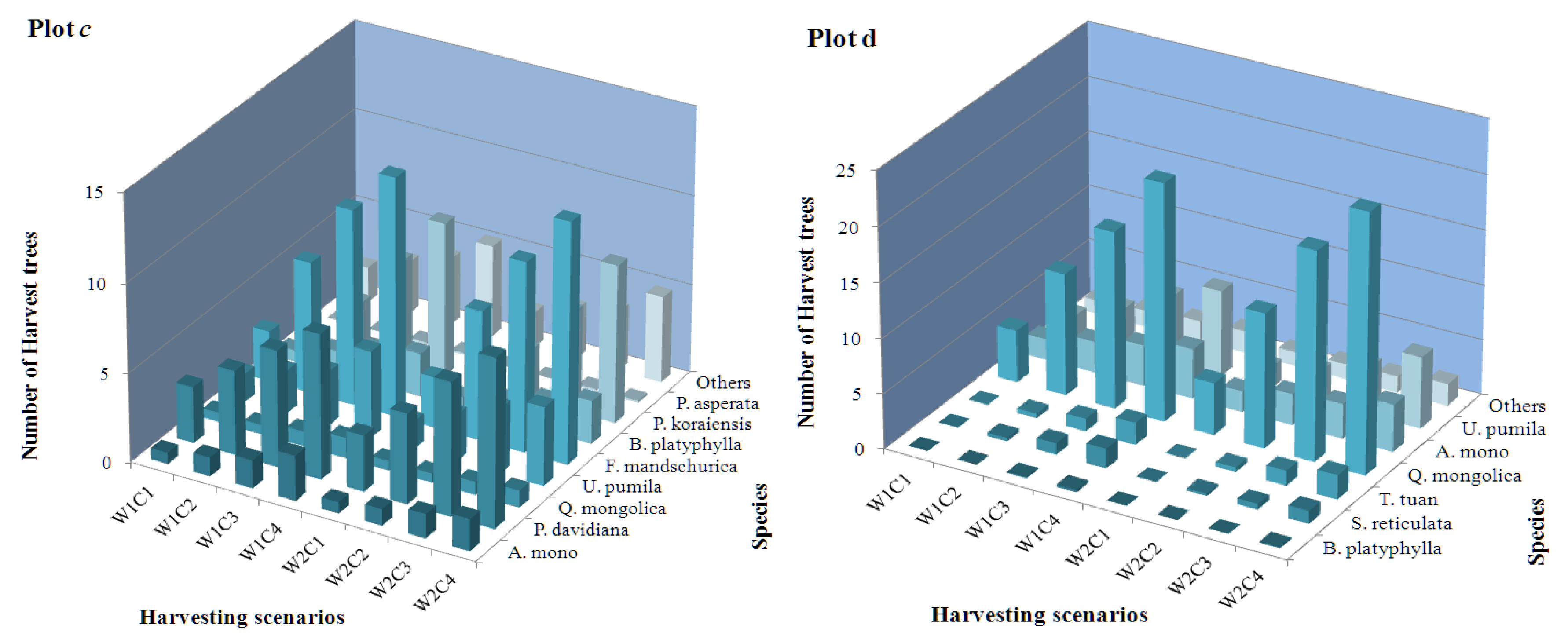
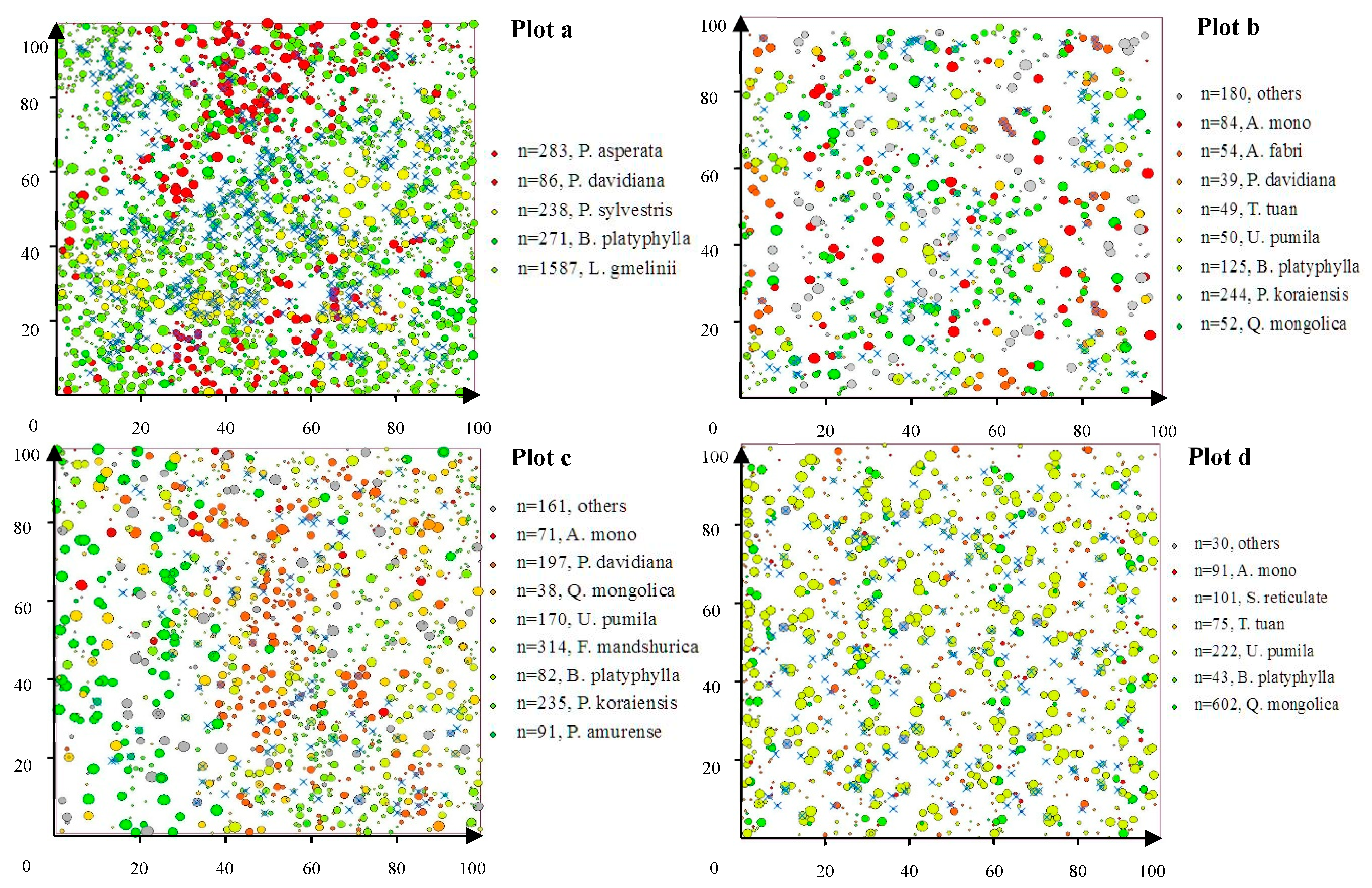
The frequency distribution of assigned harvest trees with respect to the entire core area for different tree species within the four tested plots is illustrated in Figure 3. For natural mixed larch-Betula forests, the harvest possibilities of L. gmelinii were significantly higher than those of other tree species, and were as much as 6.07% greater than those for lower harvesting intensity (i.e., removing 10% of the trees) and 28.83% higher than those for higher harvesting intensity (i.e., removing 40% of the trees) when equal weights were employed. Similarly, significantly higher harvest possibilities of P. koraiensis, namely, 6.88% of that for lower harvesting intensity and 16.09% of that for higher harvesting intensity, were observed for natural mixed Korean pine-broadleaved forest. With respect to natural oak forests, Q. mongolica was the predominant harvest tree species, accounting for approximately 6.88% of that for the lower harvesting intensity and 16.09% of that for the higher harvesting intensity. However, the distribution pattern of harvest tree species of the natural secondary forest was more complicated than that in the other three plots, in which the harvest possibility of F. mandschurica varied from 2.85% to 13.41%, that of P. davidiana varied from 3.17% to 8.13%, that of P. koraiensis varied from 0.21% to 8.66%, and that of U. pumila varied from 1.58% to 4.86%, with an increase in harvesting intensity. As emphasized here, the numerical value of the frequency distribution of the assigned harvest tree species might be different when unequal weights were employed; however, the final verdicts were all consistent with the equal weights. The spatial distribution pattern of the assigned harvest trees for the four studied plots when the harvesting intensity was 10% and unequal weights were employed, in which the improvements in the spatial structural characteristics are evident and clearly discernible with the naked eye, is illustrated in Figure 4.

4. Discussion

The spatial patterns of trees and their interactions are of paramount importance in controlling the competition status, seedling growth, and survival and crown formation of trees, and knowledge of these patterns contributes to improving our understanding of the history, functions, and future potential of a particular forest ecosystem. It is almost impossible to maintain or generate a complex and reasonable stand structure promoting stand productivity, biodiversity, and stability without considering the detailed spatial characteristics of the forest. Therefore, how to utilize thinning techniques to improve the rationality and diversity of stand fine-scale stand structure has become the main concern of forest managers. The analysis presented in this paper successfully constructed a comprehensive thinning index by weighting the widely used spatial and nonspatial structure indices. The index was then employed to evaluate and simulate the effects of different thinning intensities on four different forest types across the province of Heilongjiang in Northeast China. The obtained results indicated that the proposed comprehensive thinning index can effectively affect the structural differentiations between different forest types and alternative thinning intensities and therefore can be used as a quantitative tool to manage uneven-aged mixed forests.

Our first hypothesis, that the proposed comprehensive thinning index can reflect the structural differentiations between different forest types and alternative thinning intensities, appears to be perfectly supported by our results. Since the four studied plots were extracted from different climatic regions (Figure 1), the differentiations between their spatial and nonspatial structural characteristics were obvious. With almost similar stand basal areas (i.e., 20 m²/ha), their stem numbers and the sizes of individuals differed significantly (Table 1), in which larch-birch mixed forests had approximately twice as many trees as the others. The differences among these plots were also reflected clearly by the number of tree species, which is another traditional measure of forest structure. For the two more novel nonspatial indices (i.e., the S- and V-indices), Plot b obtained the smallest stability value and the largest vigor value, simultaneously, when compared with the other stands, indicating the unique stand vigor and stability characteristics of pine-broadleaved mixed forests, which have suffered some anthropogenic disturbances during recent decades.

Spatial attributes provided further information about the plots. The differentiations of tree neighborhood-based spatial parameters (i.e., U-, M-, and D-indices) were mainly reflected by the mixed species compositions, in which the tree size differentiations were all very uniform, and the horizontal patterns of the trees all exhibited clumped distributions, while the mingling values differed significantly from each other. Plots b and c were both stands with strongly mixed compositions; however, Plots a and d had relatively lower mingling values, both belonging to the moderate mixed composition (Table 3 and Table 4). The significant positive relationships between species richness and mingling values implied that the complexity of the neighborhood-based stand structure of the four tested plots may highly depend on the traditional measures of biodiversity, which is consistent with the results from previous studies on the comparisons of stand structure with different species compositions [26,43]. In addition, since a slight decreasing tendency of the values of the U-index with increasing stand density was observed, the number of trees per hectare might be another traditional measure of stand structure that can contribute to improving the complexity of fine-scale stand structure; however, its contribution was far less than that of the M-index. The phenomena were also detected in natural Scots pine (P. sylvestris) [44] and artificial larch (L. principis) [25] forests, both indicating that a single tree species with a large number of individuals will significantly reduce the species mingling degree and slightly increase the uniform angle degree. With respect to the distance-dependent measure, the Heygi competition index indicated that the trees grown in Plot c were suffering significantly more competition pressures than the others, mainly due to the existence of some large trees (42 trees per hectare of DBH≥30 cm) and coppice trees that shared the same (or similar) coordinates with each other (Figure 4). The differences in integral stand structure between different plots can be distinguished clearly using the proposed comprehensive thinning index. Additionally, because of the longer natural succession process (approximately 60 years) and proper human disturbance (i.e., planted P. koraiensis under canopy) in Plot c, the P-index values were significantly larger than those of Plot b, which was converted from the original pine-broadleaved mixed forests through repeated intensive selective cuttings.

Our second hypothesis that the SBFM strategy can improve the complexity and diversity of stand spatial structure at fine scales was also perfectly supported by our results. Unlike the thinning priority index provided by Gadow et al. [23], Pastorella and Paletto [7], Li et al. [26], and Ye et al. [25], which considered only part (or all) of the stand structure characteristics based on tree neighborhood relationships, the comprehensive thinning index proposed in this paper included four critical aspects with respect to stand fine-scale structures, competition status, tree vigor, and stability. The simulated results indicated that the thinning treatment based on the SBFM strategy significantly affected the spatial structure of the four tested plots to different degrees. With increasing thinning intensities, D and M both increased; however, U and H both decreased, while S and V fluctuated with intensity. These results indicated that thinning could increase the tree dominance and mixing degree and decrease the aggregation extent of the horizontal distribution and competition pressure of reference trees, which was consistent with the results from some successful practices [16,23,26]. However, the detailed response mechanisms among tree vigor, stability, and thinning intensities were more complex when the SBFM strategy was implemented, and therefore, these require further research. The differences in the P-index between different thinning intensities for most of the simulation cases were also statistically significant (Table 3 and Table 4). As emphasized here, the benefits of using the neighborhood-based parameters are that the multifaceted relations among trees are clearly defined and can be investigated very quickly and precisely. Although the distance-dependent measure of the Heygi competition index requires detailed tree coordinates in space, which usually require very time- and cost-consuming data collection methods, it can be estimated using the universal and stable power functions between the DBH and H-index of individuals, a method that has been verified for a wide range of stand characteristics [45,46]. Therefore, the application of our proposed comprehensive thinning index can not only improve the speed and accuracy of field surveys, but also reduce the subjectivity of the choice of trees to be harvested in uneven-aged mixed forests.

The final hypothesis, that there would be an optimal thinning intensity that could effectively improve the stand spatial structure characteristics, was not supported. The integral forest structure characteristics (i.e., P-index) all increased significantly, although some attributes may have been sacrificed. The P-index values increased as much as 10% or more when compared with those with no harvest, while the rates of these increases (i.e., RIP) decayed gradually with increasing thinning intensities in all four tested plots. The maximum RIP values were all observed when 10% of the trees were removed from the studied plots, indicating that removing 10% of the trees might be the most effective thinning intensity in terms of improving the integral stand structure characteristics, especially for the areas that have suffered repeated intensive selective cutting and in which the valuable trees have almost been depleted. The intensity is also coincidently satisfied with forest management policies and regulations from the State Forestry Bureau of China [47], in which harvesting for timber purposes from natural forests has been strictly prohibited, instead of allowing low-intensity tending operations to improve the quality of forest ecosystems. The assigned harvest within this intensity mainly focused on the trees with low health, lower vigor (e.g., small crown), and high competition status, while only a handful of trees were harvested for the purpose of adjusting the neighborhood-based structure (Figure 4). However, the optimal intensity from the perspective of stand structure optimization was far less than that for the purpose of promoting stand growth and yield (45% in [48]; 38%–52% in [49]), species diversity (44% in [50]), carbon sequestration and stocks (45% in [51]), and soil physical and chemical properties (30% in [52]). Therefore, the effects of removing 10% of the trees on various aspects of forest ecosystems, and the differences compared with other intensities, require more research.

The proposed comprehensive thinning index could be considered as accurate, efficient, and impersonal for selecting thinning trees in practice; however, there may be some technical reasons for the hinderance of direct application. The first, and perhaps the most important, was that two subjective weights (i.e., equal and unequal weights) were employed in the six portions of the objective function for all four plots, without considering the details of stand characteristics, management objectives, and the willingness of other stakeholders. Therefore, when one goal is weighted differently from the others, the results may also be biased. The second important technical reason was that the information regarding the vertical dimension for tree distribution was not also considered, which is also ecologically important [53,54]; thus, it would also be interesting to explore whether the inclusion of vertical structure such as the stand layer index (L) [53] or other similar indices could improve the simulation of optimizing stand structure. The last, but not least, reason is that the time and money consumed by mapping the locations of the trees usually increased geometrically with increasing sampling size.

5. Conclusions

Following the guidance of the SBFM strategy, the case study presented here proposed an accurate, efficient, and impersonal comprehensive thinning index for the selection of candidate harvesting trees by weighting the commonly used quantitative indices with respect to stand fine-scale structure, competition status, tree vigor, and tree stability. The applications of this index in evaluating and simulating the process of thinning operations for the four widely distributed forest types across the province of Heilongjiang in Northeast China indicated that the proposed comprehensive thinning index could effectively affect the structural differentiations between different forest types and alternative thinning intensities. The ranks of the diversity and complexity of integral forest structure characteristics were as natural secondary forest (0.600 and 0.638), pine-broadleaved mixed forest (0.588 and 0.623), larch-birch mixed forest (0.566 and 0.597), and natural oak forest (0.552 and 0.585) when equal and unequal weights were implemented, respectively. The marginal benefits of alternative thinning intensities on the integral forest structure showed that removing 10% of the trees from the stands was the optimal thinning intensity for optimizing the integral stand structure characteristics, in which the comprehensive thinning index could be improved by approximately 5%–11% in the four test plots. However, forest management is a long-term project in nature, and one optimization cannot solve all issues; thus, the processes of the optimization, monitoring, and evaluation of forest ecosystems should be implemented cyclically.

References

- State Forestry Bureau. National Forest Resources Continuous Inventory Technical Regulations; State Forestry Bureau: Beijing, China, 2003. (In Chinese)
- Whittaker, R.H. Evolution and measurement of species diversity. Taxon 1972, 21, 213–251. [Google Scholar] [CrossRef] [Green Version]
- Pommerening, A. Approaches to quantifying forest structures. Forestry 2002, 75, 305–324. [Google Scholar] [CrossRef]
- Barlow, J.; Gardner, T.A.; Araujo, I.S.; Avila-Pires, T.C.; Bonaldo, A.B.; Costa, J.E.; Esposito, M.C.; Ferreira, L.V.; Hawes, J.; Hernandez, M.I.M.; et al. Quantifying the biodiversity value of tropical primary, secondary, and plantation forests. Proc. Natl. Acad. Sci. USA 2007, 104, 18555–18560. [Google Scholar] [CrossRef] [Green Version]
- Eyvindson, K.; Repo, A.; Mönkkönen, M. Mitigating forest biodiversity and ecosystem service losses in the era of bio-based economy. For. Policy Econ. 2018, 92, 119–127. [Google Scholar] [CrossRef]
- State Forestry Bureau. National Forest Management Plan (2016–2050). Available online: http://www.forestry.gov.cn/uploadfile/main/2016-7/file/2016-7-27-5b0861f937084243be5d17399f5f5f71.pdf (accessed on 7 April 2020). (In Chinese)
- Pastorella, F.; Paletto, A. Stand structure indices as tools to support forest management: An application in Trentino forests (Italy). J. For. Sci. 2013, 59, 159–168. [Google Scholar] [CrossRef] [Green Version]
- Clark, P.J.; Evans, F.C. Distance to nearest neighbor as a measure of spatial relationships in populations. Ecology 1954, 35, 445–453. [Google Scholar] [CrossRef]
- Pielou, E.C. Mathematical Ecology; Wiley: New York, NY, USA, 1977. [Google Scholar]
- Ripley, B.D. Modeling spatial patterns. J. R. Stat. Soc. Ser. B Stat. Meth. 1977, 39, 172–212. [Google Scholar]
- Wiegand, T.; Moloney, K.A. Rings, circles, and null-models for point pattern analysis in ecology. Oikos 2004, 104, 209–229. [Google Scholar] [CrossRef]
- Hui, G.Y.; Gadow, K.V.; Albert, M. The neighborhood pattern-a new structure parameter for describing distribution of forest tree position. Sci. Silvae Sin. 1999, 35, 37–42. (In Chinese) [Google Scholar]
- Hui, G.Y.; Zhao, X.H.; Zhao, Z.H.; von Gadow, K. Evaluating tree species spatial diversity based on neighborhood relationships. For. Sci. 2011, 57, 292–300. [Google Scholar]
- Aguirre, O.; Hui, G.Y.; von Gadow, K.; Javier, J. An analysis of spatial forest structure using neighbourhood-based variables. For. Ecol. Manag. 2003, 183, 137–145. [Google Scholar] [CrossRef]
- Zhao, Z.H.; Hui, G.Y.; Hu, Y.B.; Li, Y.F.; Wang, H.X. Method and application of stand spatial advantage degree based on the neighborhood comparison. J. Beijing For. Univ. 2014, 36, 78–82. (In Chinese) [Google Scholar]
- Li, Y.F.; Ye, S.M.; Hui, G.Y.; Hu, Y.B.; Zhao, Z.H. Spatial structure of timber harvested according to structure-based forest management. For. Ecol. Manag. 2014, 322, 106–116. [Google Scholar] [CrossRef]
- Adams, D.M.; Latta, G.S. Effects of a forest health thinning program on land and timber values in eastern Oregon. J. For. 2004, 102, 9–13. [Google Scholar]
- Paletto, A.; Meo, I.D.; Grilli, G.; Nikodinoska, N. Effects of different thinning systems on the economic value of ecosystem services: A case-study in a black pine peri-urban forest in Central Italy. Ann. For. Res. 2017, 60, 313–326. [Google Scholar]
- Dařenová, E.; Crabbe, R.; Knott, R.; Uherkova, B.; Kadavy, J.; Darenova, E. Effect of coppicing, thinning and throughfall reduction on soil water content and soil CO2 efflux in a sessile oak forest. Silva Fenn 2018, 52. [Google Scholar]
- Gaztelurrutia, M.D.R.; Oviedo, J.A.B.; Pretzsch, H.; Magnus, L.; Ruiz-Peinado, R. A review of thinning effects on Scots pine stands: From growth and yield to new challenges under global change. For. Syst. 2017, 26, eR03S. [Google Scholar]
- Johnson, D.W.; Murphy, J.D.; Walker, R.F.; Miller, W.W.; Glass, D.W.; Todd, D.E. The combined effects of thinning and prescribed fire on carbon and nutrient budgets in a Jeffrey pine forest. Ann. For. Sci. 2008, 65, 601. [Google Scholar] [CrossRef] [Green Version]
- von Gadow, K.; Hui, G.Y. Modelling forest development. For. Sci. 1999, 57, 46–58. [Google Scholar]
- von Gadow, K.; Zhang, C.; Wehenkel, C.; Pommerening, A.; Corral-Rivas, J.; Korol, M.; Myklush, S.; Hui, G.Y.; Kiviste, A.; Zhao, X.H. Forest Structure and Diversity; Springer: Berlin, Germany, 2012; pp. 30–62. [Google Scholar]
- Song, Y.F. Individual Tree Growth Models and Competitors Harvesting Simulation for Target Tree-Oriented Management. Ph.D. Thesis, Chinese Academy of Forestry, Beijing, China, 2015. (In Chinese). [Google Scholar]
- Ye, S.X.; Zheng, Z.R.; Diao, Z.Y.; Ding, G.D.; Bao, Y.F.; Liu, Y.D.; Gao, G.L. Effects of thinning on the spatial structure of Larix principis-rupprechtii plantation. Sustainability 2018, 10, 1250. [Google Scholar] [CrossRef] [Green Version]
- Li, Y.; Hui, G.Y.; Wang, H.X.; Zhang, L.J.; Ye, S.X. Selection priority for harvested trees according to stand structural indices. iForest 2017, 10, 561–566. [Google Scholar] [CrossRef] [Green Version]
- State Forestry Bureau. Forest Resources Statistics of China; China Forestry Press: Beijing, China, 2010. (In Chinese) [Google Scholar]
- Zhang, L.Y.; Dong, L.B.; Liu, Q.; Liu, Z.G. Spatial patterns and interspecific associations during natural regeneration in three types of secondary forest in the central part of the Greater Khingan Mountains, Heilongjiang Province, China. Forests 2020, 11, 152. [Google Scholar] [CrossRef] [Green Version]
- Fu, L.Y.; Xiang, W.; Wang, G.X.; Hao, K.J.; Tang, S.Z. Additive crown width models comprising nonlinear simultaneous equations for Prince Rupprecht larch (Larix principis) in northern China. Trees 2017, 31, 1–13. [Google Scholar] [CrossRef]
- Hann, D.W. An adjustable predictor of crown profile for stand-grown Douglas-fir trees. For. Sci. 1999, 45, 217–225. [Google Scholar]
- Lu, J.; Li, F.R.; Zhang, H.R.; Zhang, S.G. A crown ratio model for dominant species in secondary forests in Maoer Mountain. Sci. Silvae Sin. 2011, 47, 70–76. (In Chinese) [Google Scholar]
- Sharma, R.P.; Vacek, Z.; Vacek, S. Modeling individual tree height to diameter ratio for Norway spruce and European beech in Czech Republic. Trees 2016, 30, 1–14. [Google Scholar] [CrossRef]
- Kamimura, K.; Gardiner, B.; Kato, A.; Hiroshima, T.; Shiraishi, N. Developing a decision support approach to reduce wind damage risk-a case study on sugi (Cryptomeria japonica (L.f.) D. Don) forests in Japan. Forestry 2008, 81, 429–445. [Google Scholar] [CrossRef] [Green Version]
- Mitchell, S.J. Wind as a natural disturbance agent in forests: A synthesis. Forestry 2013, 86, 147–157. [Google Scholar] [CrossRef] [Green Version]
- Moore, J.R. Differences in maximum resistive bending moments of Pinus radiata trees grown on a range of soil types. For Ecol. Manag. 2000, 135, 63–71. [Google Scholar] [CrossRef]
- Richards, M.; Mcdonald, A.J.S.; Aitkenhead, M.J. Optimisation of competition indices using simulated annealing and artificial neural networks. Ecol. Model. 2008, 214, 375–384. [Google Scholar] [CrossRef]
- Bettinger, P.; Tang, M. Tree-level harvest optimization for structure-based forest management based on the species mingling index. Forests 2015, 6, 1121–1144. [Google Scholar] [CrossRef]
- Hui, G.Y.; von Gadow, K.; Hu, Y.B.; Chen, B.W. Characterizing forest spatial distribution pattern with the mean value of uniform angle index. Acta Ecol. Sin. 2004, 24, 1225–1229. (In Chinese) [Google Scholar]
- Hui, G.Y.; von Gadow, K.; Hu, Y.B. The optimum standard angle of the uniform angle index. For. Res. 2004, 17, 687–692. (In Chinese) [Google Scholar]
- Pukkala, T.; Ketonen, T.; Pykäläinen, J. Predicting timber harvests from private forests-a utility maximization approach. For. Policy Econ. 2003, 5, 285–296. [Google Scholar] [CrossRef]
- Lei, X.D.; Lu, Y.C.; Peng, C.H.; Zhang, X.P.; Chang, J.; Hong, L.X. Growth and structure development of semi-natural larch-spruce-fir (Larix olgensis-Picea jezoensis-Abies nephrolepis) forests in northeast China: 12-year results after thinning. For. Ecol. Manag. 2007, 240, 165–177. [Google Scholar] [CrossRef]
- Zhu, Y.J.; Dong, X.B. Evaluation of the effects of different thinning intensities on larch forest in Great Xing’an Mountains. Sci. Silvae Sin. 2016, 52, 29–38. (In Chinese) [Google Scholar]
- Dong, L.B.; Liu, Z.G.; Ma, Y.; Ni, B.L.; Li, Y. A new composite index of stand spatial structure for natural forest. J. Beijing For. Univ. 2013, 35, 16–22. (In Chinese) [Google Scholar]
- Dong, L.B.; Liu, Z.G. Visual management simulation for pinus Sylvestris var. mongolica plantation based on optimized spatial structure. Sci. Silvae Sin. 2012, 48, 77–85. [Google Scholar]
- Béland, M.; Lussier, J.M.; Bergeron, Y.; Longpre, M.H.; Béland, M. Structure, spatial distribution and competition in mixed jack pine (Pinus banksiana) stands on clay soils of eastern Canada. Ann. For. Sci. 2003, 60, 609–617. [Google Scholar] [CrossRef] [Green Version]
- Fraver, S.; D’Amato, A.W.; Bradford, J.B.; Jonsson, B.G.; Jonsson, M. Tree growth and competition in an old-growth Picea abies forest of boreal Sweden: Influence of tree spatial patterning. J. Veg. Sci. 2014, 25, 374–385. [Google Scholar] [CrossRef]
- State Forestry Bureau. Regulations for forest tending; China Standards Press: Beijing, China, 2015. (in Chinese) [Google Scholar]
- Makinen, H.; Isomaki, A. Thinning intensity and growth of Norway spruce stands in Finland. Forestry 2004, 77, 349–364. [Google Scholar] [CrossRef] [Green Version]
- Pérezdelis, G.; Garcíagonzález, I.; Rozas, V.; Arevalo, J.R. Effects of thinning intensity on radial growth patterns and temperature sensitivity in Pinus canariensis afforestations on Tenerife Island, Spain. Ann. For. Sci. 2011, 68, 1093–1104. [Google Scholar] [CrossRef] [Green Version]
- Xu, Y.; Liu, Y.; Li, G.L. Effects of the thinning intensity on the diversity of undergrowth vegetation in Pinus tabulaeformis plantations. J. Nanjing For. Univ. 2008, 32, 135–138. (In Chinese) [Google Scholar]
- Settineri, G.; Mallamaci, C.; Mitrović, M.; Sidari, M.; Muscolo, A. Effects of different thinning intensities on soil carbon storage in Pinus laricio forest of Apennine South Italy. Eur. J. For. Res. 2018, 137, 131–141. [Google Scholar] [CrossRef] [Green Version]
- Fang, S.Z.; Lin, D.; Tian, Y.; Hong, S.X. Thinning intensity affects soil-atmosphere fluxes of greenhouse gases and soil nitrogen mineralization in a lowland poplar plantation. Forests 2016, 7, 141. [Google Scholar] [CrossRef] [Green Version]
- Cao, X.Y.; Li, J.P.; Zhou, Y.Q.; Deng, C. Stand layer index and its relations with species diversity of understory shrubs of Cunninghamia lanceolata plantations. Chin. J. Ecol. 2015, 34, 589–595. (In Chinese) [Google Scholar]
- Falster, D.S.; Westoby, M. Plant height and evolutionary games. Trends Ecol. Evol. 2003, 18, 337–343. [Google Scholar] [CrossRef]
Figure 1.
The locations and characteristics of the studied forest stands in Heilongjiang Province in Northeast China, in which Plots a–d represent the mixed larch-Betula forest, the Korean pine-broadleaved forest, the natural secondary forest, and the natural oak forest, respectively.
Figure 2.
The shapes of the sub-utility functions (fk() in Equation (7)) for tree vigor, mingling index, and dominance index (a); for stability and competition pressure (b); and for uniform angle index (c).
Figure 3.
The quantity distribution of harvested trees with respect to the entire core area for different tree species within the four tested plots, in which Plots a–d represent the mixed larch-Betula forest, the mixed Korean pine-broadleaved forest, the natural secondary forest, and the natural oak forest, respectively; symbols W1 and W2 represent the equally and unequally weighted scenarios, respectively; and C1–C4 represent the different harvesting intensities (i.e., removing 10%, 20%, 30%, or 40% of the trees).
Figure 4.
The distribution patterns of harvested trees (× with blue color) for the four studied plots when the harvesting intensity was 10% and unequal weights were employed, in which the colors of the circles indicate different tree species and their sizes indicate the diameter at breast height; n represents the number of trees of each species; and Plots a–d represent the mixed larch-Betula forest, the Korean pine-broadleaved forest, the natural secondary forest, and the natural oak forest, respectively.