Estimating Land Use and Land Cover Change in North Central Georgia: Can Remote Sensing Observations Augment Traditional Forest Inventory Data?

Abstract

Throughout the last three decades, north central Georgia has experienced significant loss in forest land and tree cover. This study revealed the temporal patterns and thematic transitions associated with this loss by augmenting traditional forest inventory data with remotely sensed observations. In the US, there is a network of field plots measured consistently through time from the USDA Forest Service’s Forest Inventory and Analysis (FIA) Program, serial photo-based observations collected through image-based change estimation (ICE) methodology, and historical Landsat-based observations collected through TimeSync. The objective here was to evaluate how these three data sources could be used to best estimate land use and land cover (LULC) change. Using data collected in north central Georgia, we compared agreement between the three data sets, assessed the ability of each to yield adequately precise and temporally coherent estimates of land class status as well as detect net and transitional change, and we evaluated the effectiveness of using remotely sensed data in an auxiliary capacity to improve detection of statistically significant changes. With the exception of land cover from FIA plots, agreement between paired data sets for land use and cover was nearly 85%, and estimates of land class proportion were not significantly different for overlapping time intervals. Only the long time series of TimeSync data revealed significant change when conducting analyses over five-year intervals and aggregated land categories. Using ICE and TimeSync data through a two-phase estimator improved precision in estimates but did not achieve temporal coherence. We also show analytically that using auxiliary remotely sensed data for post-stratification for binary responses must be based on maps that are extremely accurate in order to see gains in precision. We conclude that, in order to report LULC trends in north central Georgia with adequate precision and temporal coherence, we need data collected on all the FIA plots each year over a long time series and broadly collapsed LULC classes.

1. Introduction

Considering the numerous unintended consequences of land-use change, including the loss of biodiversity, climate feedbacks, and altered hydrologic processes [1,2], there is a growing need for land use and land cover (LULC) change information to help improve the sustainable management of Earth’s remaining resources [3]. In the United States, the US Department of Agriculture’s Forest Inventory and Analysis (FIA) Program collects information on statuses and trends in forested ecosystems across the country [4]. Since its inception in the 1920s, this program has sampled field data across the US. However, land use information was historically constrained to simple forest/non-forest classifications [5], while land cover focused mainly on resolving tree canopy cover (particularly as it related to forest land use definitions).

Motivated by events such as its transition to a nationally consistent annual inventory [6] and the refinement of forest land definitional changes, FIA has continued to expand the thematic detail in its LULC classifications [7]. More recently, the “Agricultural Act of 2014” (2014 Farm Bill, Public Law 113-79) contained a provision that specifically called for understanding and reporting on changes in LULC. Currently, trends outside of forests in the United States are monitored through the Natural Resources Conservation Service (NRCS) National Resource Inventory (NRI), which does not cover federal land, and the National Land Cover Database (NLCD), which is a modeled product [8]. Consequently, FIA has a unique niche to fill and is investigating options for enhanced collection and reporting on LULC. One option is to simply continue using the data collected on FIA’s extensive network of permanent field plots located throughout the country. But there is growing interest in the ability of remotely sensed observations to provide more frequent information about changes in LULC occurring across the US (e.g., [9,10,11,12]).

To better understand alternative LULC data, in this study, we compare the information collected on FIA plots with measurements obtained from aerial photointerpretation using the image-based change estimation (ICE) methodology [13,14,15], and the manual interpretation of Landsat images using TimeSync [16] (both described in detail in the Methods). Using data collected in FIA’s north central estimation unit of Georgia, we first compare the agreement between these three sources of LULC information, both at the plot level and in terms of the estimates they produce. We then evaluate the ability of each data source to provide temporally coherent estimates of land class status, which we define as showing realistically smooth transitions through time, as well as statistically significant net and transitional changes over varying time intervals. Finally, we assess whether auxiliary remote sensing data, through two-phase or post-stratified estimators, can be used to improve our ability to detect changes that are statistically different from zero.

2. Materials and Methods

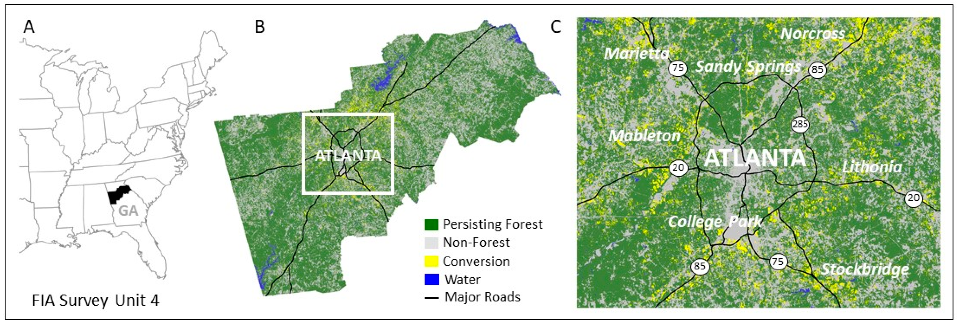
2.1. Study Area

The study area consists of 32 counties, which make up FIA’s north central estimation unit in Georgia (Figure 1). This area falls mostly in the Piedmont ecosection [17] which is considered to be an area of transition from the mostly mountainous ecoregions of the Appalachians down to the relatively flat coastal plain in the southeast. The Piedmont ecosection has an interesting LULC change history. Over the last 200 years, it has experienced several transformations, from forest to farm (mid-1700s to mid-1800s [18]), reversion to pine and hardwood woodlands (early to mid-1900s [19,20]), and now rapidly spreading urban- and suburbanization, particularly around the Atlanta-Sandy Springs-Marietta metropolitan area (mid-1900s to early 2000s [21,22]). Early on, FIA data were used to document and report on LULC changes in the state of Georgia, calling attention to the significant loss of commercial forest land to agriculture and urbanization, and projecting further declines in response to growing population needs [23]. Furthermore, the rate of conversion from forest to developed land use has been decreasing since 2007, and there was a decreasing rate in conversion from agriculture to forests until 2009, after which that rate remained stable [24].

2.2. LULC Change Observations

2.2.1. FIA Observations

A network of 1306 sample plots has been established by the FIA program across the study area at an intensity of approximately one plot every 2428 ha. Since 2000, plot data have been collected under an annual, non-overlapping panel design, where each panel consists of one-fifth of the sample plots distributed roughly equidistant throughout the population [26]. After 5 years (the cycle length in this part of the US), all plots are visited and re-measurement of plots resumes in the first panel (as depicted by the green arrows in Figure 2). At each plot location, numerous forest, tree, and stand attributes are collected. FIA’s LULC variables are collected both in the field and in the office. For example, plots previously determined to contain forest land use are assigned a LULC class by field crews, while plots determined to be non-forest are labeled in the office using aerial photography. For each plot visited in the field, data are collected on four subplots, shown as light blue circles in Figure 3.

2.2.2. ICE Observations

The image-based change estimation (ICE, [13]) process involves collecting detailed LULC change information on FIA plots using two or more dates of aerial photography collected by the National Agriculture Imagery Program (NAIP, [27]). For these analyses, ICE data were interpreted for the time periods 2010–2013, 2013–2015, and 2015–2017 (purple arrows in Figure 2). If change was seen in the two-date image pair, photo interpreters recorded LULC change information for all 45 points in the plot boundary (red triangles and white dots in Figure 3). If no change was observed, LULC change information was recorded only for the five white dots shown in Figure 3.

2.2.3. TimeSync Observations

TimeSync [16] is an interpretation tool that enables the extraction of information from more than three decades of Landsat data. Human interpretations were made on all the FIA sample plots using annual Landsat imagery, visualizations of spectral trajectories, and aerial photography through this tool. LULC and the agent of change (if any) were recorded annually on each sample plot from 1984–2017 (blue arrows in Figure 2) using the 30-m pixel intersecting the center FIA subplot (depicted by the orange box in Figure 3).

2.2.4. Thematic Detail

Each of the three data sources captured varying amounts of thematic detail in the LULC classes that were recorded. FIA observations enabled the most thematic detail, with slightly less for ICE, and the least by TimeSync. For the purposes of this paper, land use classes were collapsed into four broad categories: forest, agriculture, developed, and other non-forest. Land cover classes from each data source were collapsed into four broad land cover categories: tree, other vegetation, impervious, and water. Details of how the LULC classes were collapsed are provided in

Table A1. Crosswalk of land use categories to four broad groups used for analyses.

Land Use	FIA	TimeSync	ICE
Forest	1 Timberland	Forest	110 Forest
	2 Other forest
Agriculture	10 Agriculture	Agriculture	310 Farmland
	11 Crop	Row crop	320 Agricultural woody cropland
	12 Pasture	Orchard/tree Farm/vineyard
	13 Idle farmland		330 Windbreak/shelterbelt
	14 Orchard	Rangeland/pasture	500 Rangeland
	15 Christmas tree
	16 Maintained wildlife openings
	17 Windbreak/shelterbelt
	20 Rangeland
Developed	30 Developed	Developed Mining	410 Cultural
	31 Cultural		420 Right-of-way
	32 Right-of-way		430 Recreation
	33 Recreation		440 Mines/quarries/gravel pits
	34 Mining
Other non-forest	40 Other non-forest	Other	120 Wetland/riparian
	41 Non-veg	Non-forest wetland	121 Wetland/riparian
	42 Wetland		130 Non-forest chaparral
	43 Beach		210 Non-census water
	44 Chaparral		220 Census water
	91 Census water		323 Windbreak/shelterbelt
	92 Non-census water		900 Other non-vegetated
No data	99 Non-sampled		999 Uninterpretable

and

Table A2. Crosswalk of land use categories to four broad groups used for analyses.

Land Cover	FIA	TimeSync	ICE
Tree	01 Treeland	Trees	110 Tree—live
			120 Tree—standing dead
			150 Down and dead woody debris
Shrub and	02 Shrubland	Shrubs	130 Shrub
Other vegetation	03 Grassland	Grass/forbs/herbs	140 Other vegetation
	04 Non-vascular vegetation
	05 Mixed vegetation
	06 Agricultural vegetation
	07 Developed vegetated
Barren and	08 Barren	Barren	210 Barren
Impervious	09 Developed	Impervious	220 Impervious
Water	10 Water	Snow/ice	310 Water
		Water	320 Ice and snow
No data	99 Non-sampled		999 Uninterpretable

, respectively, in Appendix A.

2.3. Statistical Estimators

Our analyses involve three types of estimates: status, net change, and transitional change. Status captures the proportion of total land area falling in each land use or land cover category of interest by year. Net change captures the difference in proportion of a particular land use (or cover) category between two time periods, while transitional change represents what proportion of the landscape moved from one land use (or land cover) category to another over time. Estimating transitional change requires re-measured data on the same set of plots, while net change can be measured on any time interval in which a probabilistic sample of plots was observed in both time periods.

2.3.1. Status

We assume a finite population, design-based paradigm for estimating the parameters of interest. The designated area is discretized into a finite number of population units, enumerated by {1, 2, …, N} and the set of population units is denoted by U. Let the status proportion of a particular land category at time point $t$ be denoted by:

$$\begin{array}{rr}\hfill {\mu }_t& \hfill =\frac{1}{N}{\displaystyle {\displaystyle \sum }_{i\in U}}{y}_{t,i}\\ \hfill & \hfill \end{array}$$

(1)

where $y_{t,i}$ represents the proportion of unit $i$ that is the desired land category at time point $t$. A probabilistic sample, $s_t\subset U,$ is taken at time point $t$ and the estimator of ${\mu }_t,$ denoted by ${\widehat{\mu }}_t,$ is based on the observed sampled values, ${\left\{y_{t,i}\right\}}_{i\in s_t}$.

2.3.2. Net Change

The net change parameter is the difference in the proportion of a particular land category between time points t and t$-$c and is given by:

$$\begin{array}{rr}\hfill {\Delta }_{t,c}& \hfill ={\mu }_t-{\mu }_{t-c.}\\ \hfill & \hfill \end{array}$$

(2)

The net change estimator of ${\Delta }_{t,c}$ is given by $\begin{array}{rr}\hfill {\widehat{\Delta }}_{t,c}& \hfill ={\widehat{\mu }}_t-{\widehat{\mu }}_{t-c}\end{array}.$ Constructing confidence intervals for the net change parameter requires estimating the variance of ${\widehat{\Delta }}_{t,c}$. The variance of ${\widehat{\Delta }}_{t,c}$ is given by:

$$\begin{array}{rr}\hfill \mathrm{Var}\left({\widehat{\Delta }}_{t,c}\right)& \hfill =\mathrm{Var}\left({\widehat{\mu }}_t\right)+\mathrm{Var}\left({\widehat{\mu }}_{t-c}\right)-2\mathrm{Cov}\left({\widehat{\mu }}_t,{\widehat{\mu }}_{t-c}\right)\end{array}$$

(3)

where the specific form of the individual variance and covariance components depends on the form of each ${\widehat{\mu }}_j$.

2.3.3. Transitional Change

Estimating transitional change depends on remeasured data since we construct a change variable measured for year $t$ to reflect change since year $t-c.$ This change variable is an indicator function that equals one if a plot moves from a particular category to another. The transitional change parameter of moving from category A to category B is:

$${\gamma }_{t,c}=\frac{1}{N}{\displaystyle \sum }_{i\in U}{y}_{t,c,i}$$

(4)

where $y_{t,c,i}$ represents the indicator function that equals one if the plot is in category A for year $j-c$ and then category B for year $j.$ The transitional change estimator of ${\gamma }_{t,c}$ is given by ${\widehat{\gamma }}_{t,c}$.

2.3.4. Moving Average

To increase sample size and smooth out the year-to-year variability of an estimator, FIA computes a five-year moving average estimator for ${\widehat{\mu }}_j$ by pooling the sampled values from years $j$ − 4 to $j,$ which we will denote by ${\hat{\mathsf{\mu }}}_{t-4,t}$ (note that the five-year moving average is replaced by a seven- or ten-year moving average depending on inventory cycle length in different parts of the country.) While useful for depicting the status of forest attributes through time, the moving average is problematic when constructing change estimators. For example, if we want to estimate the annual net change between 2005 and 2006, then both ${\hat{\mathsf{\mu }}}_{2001,2005}$ and ${\hat{\mathsf{\mu }}}_{2002,2006}$ use the same sample data from 2002 and 2005 and only differ by the 2001 sample and the 2006 sample. Therefore, this estimator more accurately reflects the net change from 2001 to 2006, not from 2005 to 2006. The limitations and nuances of estimating net change with the moving average are discussed in [28], and alternatives given are in [29]. In the following analyses, we illustrate moving average estimates of status, but refrain from comparing net and transitional change estimates because of the temporal ambiguity.

2.4. Alternative Estimators

Our status, net change, and transitional change parameters are all population means (proportions and percentages being special cases of a mean) and can therefore be estimated with any design-based estimator of a mean. Auxiliary data, denoted by $x_{t,i}$ for unit $i$ at time t, which are known for both the sample and the population units, may also be brought in to improve precision in estimates through numerous model-assisted methodologies [30]. Note that the auxiliary data may or may not vary with time. Depending on the available auxiliary data and their relationship with the response variable, ${\widehat{\mu }}_t$, ${\widehat{\Delta }}_{t,c}$, and ${\widehat{\gamma }}_{t,c}$ can take on many different forms. If no strong relationship exists between the auxiliary data and the variable of interest, then one might consider the Horvitz–Thompson estimator [31]. If one auxiliary variable is related to the response variable, then the post-stratified estimator should be more efficient than the Horvitz–Thompson, and, if several auxiliary variables are correlated with the response, then a generalized regression estimator might be more appropriate [32]. In addition, in cases where auxiliary data are available for the sample and a subset of the population units larger than the sample itself, two-phase estimators [32] may also be considered. While the use of auxiliary data in estimates of status, net, and transitional change is not the emphasis of this paper, we include examples of these analyses to provide relevant context, as described in Section 3.2.1.

2.5. Computational Issues

All analyses were conducted in R statistical software [33]. Horvitz–Thompson and post-stratified estimates were generated using the R package mase [34]. Two-phase estimators and their estimated variances were programmed in R following [35]. Although confidence intervals for binomial data can be generated in many different ways, we used the textbook asymptotic method relying on the central limit theorem with sufficient coverage for large sample sizes.

2.6. Outline of Analyses

Using field, photo, and Landsat data collected in the north central estimation unit of Georgia, we first compare the plot-level agreement between the three sources of LULC change information. We then compare estimates of land status through time using FIA data alone, FIA data in a five-year moving average, and FIA data with ICE and TimeSync in a two-phase estimator, as well as using ICE and TimeSync as direct observations. We then assess the ability of each data set to reveal net and transitional changes over varying time intervals. Finally, we define conditions under which auxiliary data can be used to improve our ability to detect changes that are statistically different from zero through post-stratification. In conclusion, we recommend the best use of these data sets for inventory and monitoring purposes.

3. Results

3.1. Agreement between Observations at Plot Level

Whether alternative data sources are used as auxiliary data in model-assisted estimators, or as the response variable themselves, it is important to first understand the agreement in class assignments between them. We examined the percent agreement between plots paired from the three different data sources and averaged them over the timespan. In

Table 1. Plot-level agreement between two and three sources of land use and land cover information collected on FIA plots. The lower overall agreement across the three data sets implies that the pairwise agreement occurs on different plots across the three pairings.

	LU		LC
	Percent Agreement	Timespan	Percent Agreement	Timespan
All	82.4	2010, 2013, 2015	69.7	2013, 2015
FIA-ICE	87.0	2010, 2013, 2015	75.8	2013, 2015
imeSync	88.5	2000–2016, annually	75.5	2013–2016, annually
ICE-TimeSync	87.4	2010, 2013, 2015	84.6	2010, 2013, 2015

, we see that agreement on land use between pairs of data sources never falls below 87 percent, and where all three data sources are available, agreement still equals 82.4%, on average. Land cover information was available for only a few years for both FIA and ICE, so the comparisons span fewer years. As with land use, agreement between ICE and TimeSync is quite high, at around 85% for three observation years. However, agreement between all three data sources is lower than that seen in the land use comparisons.

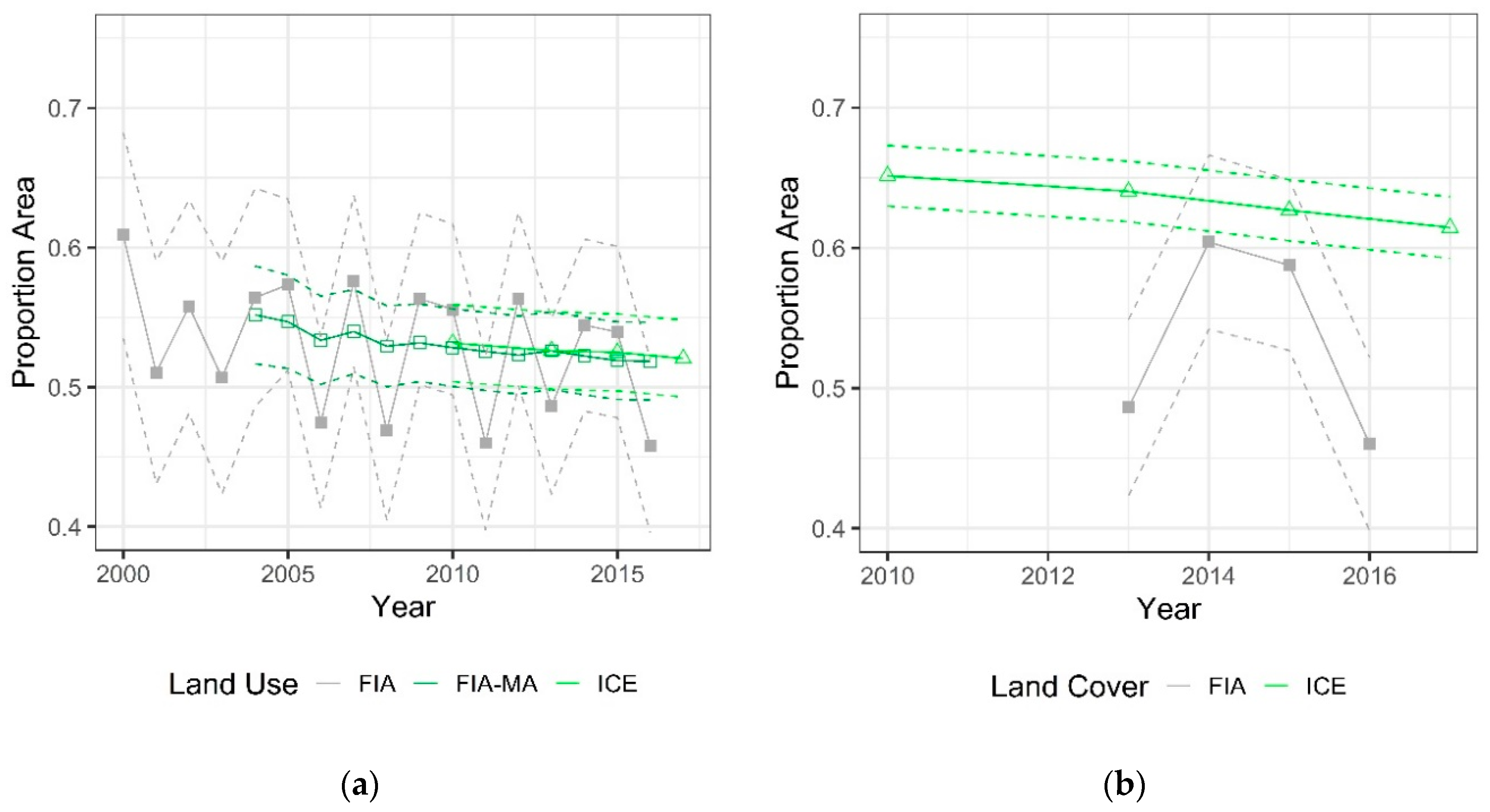
3.2. Estimates of LULC Status

3.2.1. FIA Annual Estimates

Before considering estimates of net or transitional change, it is instructive to look at the challenges in estimating LULC proportions across the landscape in any given year using FIA data as the response variable, either alone or assisted by auxiliary information. First, Figure 4a illustrates the annual estimates of the proportion of land area under forest land use, by year, using FIA data alone in a Horvitz–Thompson estimator. The large confidence intervals, along with the variability between annual samples collected in any one sub-panel (e.g., one-fifth of the FIA plots collected each year), make it difficult to decipher any meaningful trend in forest land use. Bringing in ICE data (collected on all the FIA plots in two- to three-year intervals) as phase 1 in a two-phase estimator reduces the size of the annual confidence intervals and, at first glance, suggests a smoothing effect on the inter-annual variability (Figure 4b). However, the 2010 and 2015 estimates were constructed from the exact same panels of FIA data, and the 2013 annual estimate just happened to lie close to the 2010/2015 estimates. Figure 4c, illustrating the effects of using TimeSync data as phase one in a two-phase estimator, gives a more complete story of the limitations of this two-phase approach. Again, we see a substantial reduction in the size of the confidence intervals, but this does not alleviate the year-to-year variability caused by using a different subset of plots for each year. The finding here is that using the annual FIA data themselves as a response does not provide meaningful estimates of status through time, even when aided with the ICE or TimeSync data through two-phase estimators.

3.2.2. Considering Remotely Sensed Observations

Given that the annual estimates of the proportion of area cannot be made “smooth”, even in the best-case scenario where auxiliary data are in very high agreement with the response, we turn to using the ICE and TimeSync data as the response to help alleviate the sampling variability caused by using only one-fifth of the FIA plots each year (see Section 3.2.1 above). For FIA data alone, this means using the five-year moving average and comparing that with estimates of LULC obtained directly from the ICE and TimeSync observations.

In Figure 5a, we see that using a five-year moving average (in medium green squares) is more interpretable than the annual estimates obtained using just single panels of FIA data (shown in closed gray squares, with confidence intervals dashed). ICE (in light green triangles, Figure 5a) tells a compatible story for the 2010, 2013, 2015, and 2017 dates. It has as narrow a confidence interval as the moving average, but is specific to the photo years observed and extends the observation period. Additionally, note that the FIA moving average (shown in Figure 5a) truncates our temporal window by four years at the beginning of the time series.

As already noted in our agreement analyses above, FIA and ICE land cover are only moderately related (Table 1). FIA data are not informative for tree land cover in this example because data only began being collected in 2013 so we cannot construct a meaningful five-year moving average. ICE (in light green triangles, Figure 5b), however, suggests a slowly decreasing trend.

Turning our attention to TimeSync in Figure 6, we use TimeSync observations to estimate the proportion of area in each of the four major land use (a) and land cover (b) categories through time. Notice that, from here on, we shift to displaying the long time series of estimates as both lines and points, rather than individual points, to make the interpretation of results more visually apparent. The estimates from TimeSync suggest a (slowing) decline in both forest and agricultural land use with a (slowing) increase in developed land area. Similarly for land cover, TimeSync suggests a decline in tree cover with increases in both impervious cover and other vegetation. ICE estimates (shown as triangles) are also superimposed in this figure to reiterate the close agreement in estimates obtained from these two data sets. While both Figure 6a,b suggest a compelling and coherent LULC change story for north central Georgia, more rigorous analyses of net and transitional change result in even more temporal and thematic detail. In addition, estimates produced from TimeSync for the forest land use proportion were not significantly different than those obtained from the FIA moving average or ICE, nor were they significantly different from the ICE tree cover estimates. The most notable difference is the length of the time series information available from TimeSync and the decreasing trends it suggests for both forest land use and tree cover.

3.3. Change Estimates

3.3.1. Net Change

In Figure 7, we see estimates of net proportion change in forest LULC with 95% confidence intervals from FIA data at five-year intervals and ICE for the 2–3 year NAIP cycle. This means that the value graphed for year t reflects the difference in land use proportion at time t minus that at time t minus whatever interval is specified. Neither of the sources was able to detect significant change (i.e., change estimates significantly different from zero) except in the 2009–2014 interval, where the FIA data produced a significantly negative estimate.

Similarly, net change in land use from TimeSync was explored at a variety of year intervals. The annual pattern is somewhat erratic, but our ability to detect change is enhanced as we increase interval length from annual to 5 years in Figure 8a, where we see more clearly the patterns of forest and agriculture loss coupled with a gain in urban land use for the majority of the observation period, with an apparent stabilization starting in 2013.

As might be expected, net change in land cover was more variable because use is an inherently more stable attribute. Figure 8b shows net land cover change over a five-year interval, revealing a significant but irregular loss in tree cover and a gain in impervious vegetation over time. Other vegetation is a difficult trend to decipher because it contains both agricultural and urban/suburban vegetation types. Of interest is the significant loss in tree cover late in the time series despite the apparent stability of forest land use (Figure 8a) for the same years, likely due to harvesting. It is interesting to note that the trends in land cover loss and gain are noticeably different when the change interval is increased from 5 to 10 years.

3.3.2. Transitional Change

Turning our attention to transitional change (i.e., transition from one specific use or cover class to another), we are able to refine information gleaned from the analysis of net change. Transitional change tells a clear story about land use change in north central GA; over the last 30 years, there has been a significant transition from forest to urban land use (Figure 9a). The rate of transition increased from 1984 through to approximately 2002, and that rate has been declining ever since, with a loss significantly greater than zero for all years except the most recent. The transition from treed land cover to impervious and other vegetation varies, but is significantly greater than zero throughout the time series, with no strong indication of increasing or decreasing long-term rates (Figure 9b).

3.4. Enhancing Detectability of Significant Change through Post-Stratification

In the sections above, we explored ways in which we could improve precision in various estimates through two-phase estimators, through increasing sample size by using observations on all FIA plots, and by changing the temporal observation window. The ultimate goal is to improve our ability to detect significant net and transitional changes. One more approach is to use auxiliary data, representing change in the landscape, in a post-stratified estimator. The use of such data (such as a land cover change map) could potentially decrease the variance in estimates of net and transitional change and might improve our ability to detect change that is significantly different from zero. However, the interplay between estimating a rare change event on the landscape and the potential gains in precision through post-stratification are best understood through simple graphical analyses based directly on variance formulae for a binary response. The relationship between map accuracy and efficiency gains through post-stratification has been explored in detail [36]. Here, we provide a simple analysis relevant to rare change events and common map accuracy expectations.

Let n be the sample size and p be the proportion of the population affected by the change event of interest. Then, the estimated standard error of a Horvitz–Thompson estimator, with equal probability of selection and ignoring the population correction factor, can be expressed as:

$${\mathrm{SE}}_{HT}=\sqrt{p\ast \left(1-p\right)/\left(n-1\right)}$$

(5)

Next, let $n_1$ be the sample size in stratum 1, $n_2$ the sample size in stratum 2, $w_1$ the proportion of the population in stratum 1, $w_2$ the proportion of the population in stratum 2, $p_1$ the proportion of the population affected by the change event of interest in stratum 1, and $p_2$ the proportion of the population affected by the change event of interest in stratum 2. Ignoring the finite population correction factor and a small adjustment for random sample sizes within post-strata, the estimated standard error for a post-stratified estimate of population proportion with two strata can be expressed in a simplified form:

$$S{E}_{ps}=\sqrt{w_1{}^2\left[\frac{p_1\ast \left(1-p_1\right)}{\left(n_1-1\right)}\right]+w_2{}^2\left[\frac{p_2\ast \left(1-p_2\right)}{\left(n_2-1\right)}\right]}$$

(6)

Assume we are interested in some change that occurs on a proportion p of the population. Next, assume we have a disturbance map that we will use for post-stratification that reflects this change with an accuracy of $a_1$ in the change stratum and $a_{2 }$ in the no-change stratum. Additionally, assume we have a sample size of n. In order to simulate the potential gains in precision through post-stratification over using the Horvitz–Thompson estimator, we first need to translate map accuracy metrics for the two strata into the expected weights, proportions and sample sizes we would expect to find under different map accuracy scenarios. To do this, we first look at a confusion matrix (

Table 2. Confusion matrix populated with formulae for solving for standard error rates expected under varying map accuracy scenarios.

Truth Predicted	1	2	Total
1	$n_{11}=n_{.1}{a}_1$	$n_{12}=n_{.2}\left(1-a_2\right)$	$n_{1.}=n_{11}+n_{12}$
2	$n_{21}=n_{.1}\left(1-a_1\right)$	$n_{22}=n_{.2}{a}_2$	$n_{2.}=n_{21}+n_{22}$
Total	$n_{.1}=np$	$n_{.2}=n\left(1-p\right)$	n

) from which map accuracy metrics can be generated. Let us say that map class 1 targets the change event of interest, and map class 2 targets the absence of that change event. In our simulation, for any given n, p, and producer’s accuracies by map class ($a_1 \mathrm{and} a_2)$, the row totals can be computed, followed by the four interior cells and, lastly, the column totals.

From there, the elements in the estimated standard error under post-stratification in equation X can be calculated as follows: $w_1=\frac{n_{1.}}{n}, w_2=\frac{n_{2.}}{n} ,p_1=\frac{n_{11}}{n_{1.}} , p_2=\frac{n_{22}}{n_{2.}}$.

In Figure 10, we compare the standard errors we get with just a Horvitz–Thompson estimator (black solid line) versus those using a post-stratified estimator under varying map accuracies. In practice, errors of omission in a no-change stratum are often typically very low, so we conservatively fix $a_2$ to be a very generous 95%. We then vary the accuracies within the change stratum consistent at extremely optimistic levels of 95% (blue), 85% (green), and 75% (purple). Given this optimistic setting, we see that the post-stratified estimator does substantially better than Horvitz–Thompson when the change event of interest occupies more than 20% of the landscape. However, as that event becomes increasingly rare, the benefit of post-stratification diminishes rapidly, as shown in Figure 10b. The upshot of this analysis is that maps of landscape change have to be extremely accurate in order to show any modest gains through post-stratification for rare events. Given that the best change maps can currently detect change accurately only 50%–80% of the time [37], these graphs illustrate that the use of these products as post-strata will not noticeably improve precision for rare phenomena. Hence, change maps at these accuracies cannot be expected to improve our ability to derive estimates of change that are significantly different from zero.

3.5. Compilation of Results

Table 3. Success of variations on our three data sources in delivering interpretable/significant estimates of proportion area and change through time, where ✓ indicates success, and X indicates no success. Note that the addition of two-phase estimates would not change the rating for the FIA panel data. Neither would the addition of a relatively accurate (e.g., 85%) post-stratified layer change the results for any of the data sets.

Source	Interpretable Proportion	Significant Net Change	Significant Transitional Change
FIA—panel	X	X	X X
FIA—moving average	✓	X	X
ICE	✓	✓-	X
TS—three-year interval	✓	✓-	✓
TS—five-year interval	✓	✓	✓

provides a summary of how data from the three data sources performed in their ability to portray an interpretable story and detect significant change through time in north central Georgia.

4. Discussion

Even with generalized land use and cover classes, the trends in north central Georgia presented here are unprecedented and add insight into the dynamics between forests and the pressures on them. Throughout the last three decades, this study area has experienced significant loss in forest land and tree cover, a trend also documented by [38]. The rate of transition from forest to urban (with accompanying transition of treed land to impervious and other vegetation) increased dramatically from 1984 until 2002, then the rate slowed then flattened in later years. For context, the proportion of forest in this area of Georgia increased approximately threefold from the 1930s to the 1980s [39], a change almost entirely due to the abandonment of agricultural lands. This area has long been the site of dynamic land use.

In order to decipher LULC trends in north central Georgia, we not only needed a sufficient sample size (i.e., the complete set of FIA plots instead of a single panel), but also a wide enough time interval (five-year interval instead of annual), and class simplicity (four classes instead of many). Understanding analytical limitations about true annual change is important.

There was strong agreement between the observations of land use collected by FIA, ICE, and TimeSync, with equally strong agreement between TimeSync and ICE for land cover. This opens the door to using these remotely sensed observations directly for estimation. One immediate source of such data would be the national simple random sample of TimeSync data (n = 25,000 locations) jointly collected by the US Forest Service’s Landscape Change Monitoring System and the US Geological Survey’s Land Change Monitoring, Assessment, and Projection projects [12]. To maximize agreement, some level of harmonization will be required to account for slight differences in class definitions and collection protocols among the various data sources.

Annual single-year panels of FIA data (representing 20% of the FIA sample in Georgia), were not sufficient for producing estimates of LULC proportions though time, nor for detecting significant net or transitional change. The moving average plays the role of a “poor man’s intensification”, in that it reduces SEs and also acts as a smoother, which helps identify significant trends over time. However, limitations to the moving average include the inability to target specific dates over which change has occurred and the inevitable lag in detecting increases or decreases due to smoothing.

Improving FIA panel data alone with two-phase estimators (using ICE or TimeSync in phase 1) will reduce variance in estimates, but will not smooth the inter-panel variability enough to make estimates through time meaningful. If ICE and TimeSync are not to be used as auxiliary data in model-assisted estimators, then they would no longer need to be collected independently of FIA observations. Rather, FIA plot information could be used to augment interpretations made from remotely sensed data.

Our inability to improve the detectability of significant net or transitional changes using auxiliary data in post-stratified estimators is a function of how rare those change events are, and how accurately the maps used for post-stratification reflect those rare events. Even atypically high accuracies of 85% will do little to improve precision in estimates of rare (<5% of the landscape) events. It is interesting that the covariance term between two points in time shrinks the variance and aids in detectability more than introducing auxiliary data through post-stratification.

Given the already strong agreement between the three data sets for land use, the need for sufficient sampling intensity in space and time, and the lack of gains in keeping remotely sensed data independent of the plot data for purposes of estimation, the stage is set for FIA to embrace a harmonized LULC change system. While data collected through TimeSync alone revealed the temporal patterns and transitions between collapsed classes, bringing all the evidence to bear (from the ground, air photos, and Landsat) to reconstruct the history on all its plots will result in a more comprehensive assessment of LULC change.

5. Conclusions

Using data collected in the north central section of Georgia, we compare combinations of three LULC data sets, including those from FIA plots, ICE, and TimeSync. We conclude that, in order to report LULC trends in north central Georgia with adequate precision and temporal coherence, we need data collected on all the FIA plots each year over a long time series and broadly collapsed LULC classes. This emphasizes the need for sufficient sampling intensity in space and time, and it calibrates expectations about thematic precision in estimates. Even with the generalized LULC classes, the annualized trends presented by this paper are unprecedented and add insight into the dynamics between forests and the pressures on them through time. We illustrate the limitations of using remotely sensed observations only as auxiliary data through post-stratification and two-phase estimators. These limitations highlight the benefits of an alternative approach: integrating harmonized ground, Landsat, and aerial imagery via a single enhanced plot interpretation process.

References

1. Vitousek, P.M.; Mooney, H.A.; Lubchenco, J.; Melillo, J.M. Human domination of earth’s ecosystems. Science 1997, 277, 494–499. [Google Scholar] [CrossRef] [Green Version]
2. DeFries, R.S.; Foley, J.A.; Asner, G.P. Land-use choices: Balancing human needs and ecosystem function. Front. Ecol. Environ. 2004, 2, 249–257. [Google Scholar] [CrossRef]
3. Bechtold, W.A.; Patterson, P.L. (Eds.) The Enhanced Forest Inventory and Analysis Program—National Sampling Design and Estimation Procedures; Gen. Tech. Rep. SRS-80; U.S. Department of Agriculture, Forest Service, Southern Research Station: Asheville, NC, USA, 2005; p. 85.
4. Turner, B.L., II; Lambin, E.F.; Reenberg, A. The emergence of land change science for global environmental change and sustainability. Proc. Natl. Acad. Sci. USA 2007, 104, 20666–20671. [Google Scholar] [CrossRef] [Green Version]
5. LaBau, V.J.; Bones, J.T.; Kingsley, N.P.; Lund, H.G.; Smith, W.B. A history of the forest survey in the United States: 1830–2004; FS-877; U.S. Department of Agriculture, Forest Service: Washington, DC, USA, 2007; p. 82.
6. Gillespie, A.J.R. Rationale for a national annual forest inventory program. J. For. 1999, 97, 16–20. [Google Scholar]
7. Oswalt, S.N.; Smith, W.B.; Miles, P.D.; Pugh, S.A. Forest Resources of the United States, 2017: A technical document supporting the Forest Service 2020 RPA Assessment; Gen. Tech. Rep. WO-97; U.S. Department of Agriculture, Forest Service: Washington, DC, USA, 2019; p. 223.
8. Nelson, M.D.; Riitters, K.H.; Coulston, J.W.; Domke, G.M.; Greenfield, E.J.; Langner, L.L.; Nowak, D.J.; O’Dea Claire, B.; Oswalt, S.N.; Reeves, M.C.; et al. Defining the United States land base: A technical document supporting the USDA Forest Service 2020 RPA assessment; Gen. Tech. Rep. NRS-191; U.S. Department of Agriculture, Forest Service, Northern Research Station: Madison, WI, USA, 2020; p. 70.
9. Schroeder, T.A.; Healey, S.P.; Moisen, G.G.; Frescino, T.S.; Cohen, W.B.; Huang, C.; Kennedy, R.E.; Yang, Z. Improving estimates of forest disturbance by combining observations from Landsat time series with U.S. Forest Service Forest Inventory and Analysis data. Remote Sens. Environ. 2014, 154, 61–73. [Google Scholar] [CrossRef]
10. Gray, A.N.; Cohen, W.B.; Yang, Z.; Pfaff, E. Integrating TimeSync disturbance detection and repeat forest inventory to predict carbon flux. Forests 2019, 10, 984. [Google Scholar] [CrossRef] [Green Version]
11. Lister, A.; Lister, T.; Weber, T. Semi-automated sample-based forest degradation monitoring with photointerpretation of high-resolution imagery. Forests 2019, 10, 896. [Google Scholar] [CrossRef] [Green Version]
12. Pengra, B.W.; Stehman, S.V.; Horton, J.A.; Dockter, D.J.; Schroeder, T.A.; Yang, Z.; Cohen, W.B.; Healey, S.P.; Loveland, T.R. Quality control and assessment of interpreter consistency of annual land cover reference data in an operational national monitoring program. Rem. Sens. Envr. 2020, 238. [Google Scholar] [CrossRef]
13. Webb, J.; Brewer, C.K.; Daniels, N.; Maderia, C.; Hamilton, R.; Finco, M.; Megown, K.A.; Lister, A.J. Image-based change estimation for land cover and land use monitoring. In Moving from Status to Trends: Forest Inventory and Analysis (FIA) Symposium 2012; Morin, R.S., Liknes, G.C., Eds.; Gen. Tech. Rep. NRS-P-105; U.S. Department of Agriculture, Forest Service, Northern Research Station: Newtown Square, PA, USA, 2012; pp. 46–53. [Google Scholar]
14. Frescino, T.S.; Moisen, G.G.; Megown, K.A.; Nelson, V.J.; Freeman, E.A.; Patterson, P.L.; Finco, M.; Brewer, K.; Menlove, J. Nevada Photo-Based Inventory Pilot (NPIP) photo sampling procedures; Gen. Tech. Rep. RMRS-GTR-222; U.S. Department of Agriculture, Forest Service, Rocky Mountain Research Station: Fort Collins, CO, USA, 2009; p. 30.
15. Patterson, P.L. Photo-based estimators for the Nevada photo-based inventory; Res. Pap. RMRS-RP-92; U.S. Department of Agriculture, Forest Service, Rocky Mountain Research Station: Fort Collins, CO, USA, 2012; p. 14.
16. Cohen, W.B.; Yang, Z.Q.; Kennedy, R. Detecting trends in forest disturbance and recovery using yearly Landsat time series: 2. TimeSync -- Tools for calibration and validation. Remote Sens. Environ. 2010, 114, 2911–2924. [Google Scholar] [CrossRef]
17. Omernik, J.M.; Griffith, G.E. Ecoregions of the conterminous United States: Evolution of a hierarchical spatial framework. Environ. Manag. 2014, 54, 1249–1266. [Google Scholar] [CrossRef]
18. Edwards, L. Environmental history of Georgia: Overview. New Georgia Encycl. 2018. Available online: https://www.georgiaencyclopedia.org/articles/geography-environment/environmental-history-georgia-overview (accessed on 20 July 2020).
19. Hart, J.F. Land use change in a Piedmont county. Ann. Assoc. Am. Geogr. 1980, 70, 492–527. [Google Scholar] [CrossRef]
20. Cowell, C.M. Historical change in vegetation and disturbance on the Georgia Piedmont. Am. Midl. Nat. 1998, 140, 78–89. [Google Scholar] [CrossRef]
21. Miller, M.D. The impact of Atlanta’s urban sprawl on forest cover and fragmentation. Appl. Geogr. 2012, 34, 171–179. [Google Scholar] [CrossRef]
22. U.S. Department of Agriculture. Georgia’s Land: Its Use and Condition, 4th ed.; Natural Resources Conservation Service, Athens, GA, and Center for Survey Statistics and Methodology, Iowa State University: Ames, IA, USA, 2016.
23. Sheffield, R.M.; Knight, H.A. Georgia’s Forests; Resour. Bull. SE-73; U.S. Department of Agriculture, Forest Service, Southeastern Forest Experiment Station: Asheville, NC, USA, 1984; p. 92.
24. Brandeis, T.J.; McCollum, J.M.; Hartsell, A.J.; Brandeis, C.; Rose, A.K.; Oswalt, S.N.; Vogt, J.T.; Vega, H.M. Georgia’s Forests 2014; Resour. Bull. SRS-209; U.S. Department of Agriculture, Forest Service, Southern Research Station: Ashville, NC, USA, 2016; p. 78.
25. Schleeweis, K.G.; Moisen, G.G.; Schroeder, T.A.; Toney, C.; Freeman, E.A.; Goward, S.N.; Huang, C.; Dungan, J.L. US National Maps Attributing Forest Change: 1986–2010. Forests 2020, 11, 653. [Google Scholar] [CrossRef]
26. Reams, G.A.; Smith, W.D.; Hansen, M.H.; Bechtold, W.A.; Roesch, F.A.; Moisen, G.G. The forest inventory and analysis sampling frame. In The Enhanced Forest Inventory and Analysis Program—National Sampling Design and Estimation Procedures; Bechtold, W.A., Patterson, P.L., Eds.; Gen. Tech. Rep. SRS-80; U.S. Department of Agriculture, Forest Service, Southern Research Station: Asheville, NC, USA, 2005; pp. 11–26. [Google Scholar]
27. NAIP Imagery. Available online: http://www.fsa.usda.gov/programs-and-services/aerial-photography/imagery-programs/naip-imagery/index (accessed on 6 March 2017).
28. Van Deusen, P.C. Modeling trends with annual survey data. Can. J. For. Res. 1999, 29, 1824–1828. [Google Scholar] [CrossRef]
29. Van Deusen, P.C. Alternatives to the moving average. In Proceedings of the 2nd annual Forest Inventory and Analysis Symposium, Salt Lake City, UT, USA, 17–18 October 2000; Reams, G.A., McRoberts, R.E., Van Deusen, P.C., Eds.; Gen. Tech. Rep. SRS-47; U.S. Department of Agriculture, Forest Service, Southern Research Station: Asheville, NC, USA, 2001; pp. 90–93. [Google Scholar]
30. McConville, K.S.; Moisen, G.G.; Frescino, T.S. A Tutorial on Model-Assisted Estimation with Application to Forest Inventory. Forests 2020, 11, 244. [Google Scholar] [CrossRef] [Green Version]
31. Horvitz, D.G.; Thompson, D.J. A generalization of sampling without replacement from a finite universe. J. Am. Stat. Assoc. 1952, 47, 663–685. [Google Scholar] [CrossRef]
32. Särndal, C.E.; Swensson, B.; Wretman, J. Model Assisted Survey Sampling; Springer: New York, NY, USA, 1992. [Google Scholar]
33. R Core Team. R: A Language and Environment for Statistical Computing. R Foundation for Statistical Computing, Vienna, Austria. 2019. Available online: https://www.R-project.org/ (accessed on 20 July 2020).
34. McConville, K.S.; Tang, B.; Zhu, G.; Cheung, S.; Li, S. Mase: Model-Assisted Survey Estimators. 2018. Available online: https://cran.r-project.org/web/packages/mase (accessed on 1 June 2020).
35. Cochran, W.G. Sampling Techniques; John Wiley & Sons: Hoboken, NJ, USA, 1977. [Google Scholar]
36. Czaplewski, R.L.; Patterson, P.L. Classification accuracy for stratification with remotely sensed data. For. Sci. 2003, 49, 402–408. [Google Scholar]
37. Cohen, W.B.; Healey, S.P.; Yang, Z.; Stehman, S.V.; Brewer, C.K.; Brooks, E.B.; Gorelick, N.; Huang, C.; Hughes, M.J.; Kennedy, R.E.; et al. How similar are forest disturbance maps derived from different Landsat time series algorithms? Forests 2017, 8, 98. [Google Scholar] [CrossRef]
38. Yang, X.; Lo, C.P. Using a time series of satellite imagery to detect land use and land cover changes in the Atlanta, Georgia metropolitan area. Int. J. Remote Sens. 2002, 23, 1775–1798. [Google Scholar] [CrossRef]
39. Turner, M.G.; Ruscher, C.L. Changes in landscape patterns in Georgia, USA. Landsc. Ecol. 1988, 1, 241–251. [Google Scholar] [CrossRef]
Figure 1. Study area consisting of the Forest Inventory and Analysis survey unit 4 in north central Georgia, USA (black shading, Panel A) surrounding the greater Atlanta metropolitan area (Panel B). The land classification maps shown in Panels B and C identify areas of persisting forest (green) and potential forest conversion (yellow) occurring between 1987 and 2010 (adapted from [25]). Developed from Landsat time series, the maps estimate that nearly 75,000 ha of forest were converted from forest to other land uses during the 23-year period of study. Much of the conversion is concentrated along major roadways, as seen in Panel C.
Forests 11 00856 g001
Figure 2. The percentage of plots in FIA’s quasi-systematic grid that were sampled under each of the three land use and land cover change observation systems by year pairings. Percentages on the y-axis indicate the proportion of the population sampled at each time step (x-axis). Older periodic inventories conducted by FIA are not included in these analyses.
Forests 11 00856 g002
Figure 3. The spatial scale of plot data collected under the three different observation systems. FIA plots involve field data collection within four subplots, depicted by light blue circles. Image-based Change Estimation plots make observations on a sample of dots within a 0.61 hectare circle (light green) surrounding the FIA subplots. For areas with no change from one time period to the next, data are collected only on the five white dots. For plots where change is present, data are collected on all 45 dots (white dots and red triangles combined). Finally, for TimeSync, observations are made for the 30-m pixel intersecting the center FIA subplot, depicted by an orange box.
Forests 11 00856 g003
Figure 4. (a) Estimates of the proportion of land area in forest use derived with annual FIA data, (b) annual FIA data with ICE in phase 1, and (c) annual FIA data with TimeSync in phase 1 of a two-phase estimator. FIA estimates are shown as solid gray lines with confidence intervals as light gray dashed lines. ICE and TimeSync estimates are shown as green triangles and circles, respectively, with confidence intervals as dashed green lines.
Forests 11 00856 g004
Figure 5. (a) The estimated proportion of land area in forest land use, with 95% confidence interval, by year using FIA plots alone (gray closed squares), FIA moving average (medium green open squares), and ICE (light green open triangles). (b) The same as (a) but for tree cover. Note that FIA land cover data were only collected for 2013-2016 so the five-year moving average could not be calculated.
Forests 11 00856 g005
Figure 6. (a) The estimated proportion of land area in forest (green), agriculture (yellow), developed (red), and other (blue) land use, with 95% confidence intervals, by year, using TimeSync observations. (b) The estimated proportion of land area in tree (green), other vegetation (yellow), barren and impervious (red), and water (blue) land cover, with 95% confidence intervals, by year, using TimeSync observations. ICE estimates are superimposed on both graphs as open triangles.
Forests 11 00856 g006
Figure 7. Estimates of percent net change (a) in forest land use and (b) in tree cover with 95% confidence intervals from FIA data (gray closed squares) at five-year intervals and ICE (green open triangles) at 2–3 year intervals.
Forests 11 00856 g007
Figure 8. Over five-year intervals, (a) net land use change for forest (green), agriculture (yellow), developed (red), and other (blue) land use and (b) net land cover change for in tree (green), other vegetation (yellow), barren and impervious (red), and water (blue) with 95% confidence intervals from TimeSync observations. Note that for a five-year interval, the value in year t reflects the difference in land use/cover proportion at time t minus that at time t-5.
Forests 11 00856 g008
Figure 9. Transitional change from (a) forest land use and (b) tree land cover with 95% confidence intervals at five-year intervals from TimeSync observations.
Forests 11 00856 g009
Figure 10. (a) Proportions (p) of change on the landscape and the expected standard errors using a Horvitz–Thompson estimator (black solid line) versus those using a post-stratified estimator, with change/no-change strata at varying map accuracies. Errors of omission in a no-change stratum are fixed at 95%. Accuracies within the change stratum are fixed at 95% (blue), 85% (green), and 75% (purple). (b) The same as (a) but zoomed in on small proportions.
Forests 11 00856 g010