A Numerical Approach to Estimate Natural Frequency of Trees with Variable Properties


1
Department of Civil and Environmental Engineering, Western University, London, ON N6A 5B9, Canada
2
Timberlands Limited, Rotorua 3040, New Zealand
*
Author to whom correspondence should be addressed.
Forests 2020, 11(9), 915; https://0-doi-org.brum.beds.ac.uk/10.3390/f11090915
Submission received: 3 July 2020
/
Revised: 13 August 2020
/
Accepted: 18 August 2020
/
Published: 21 August 2020
(This article belongs to the Special Issue Wind Impacts on Forests and Trees in a Changing Climate—A Special Issue in Collaboration with the IUFRO Working Party 8.03.06)
Abstract
:Free vibration analysis of a Euler-Bernoulli tapered column was conducted using the finite element method to identify the vibration modes of an equivalent tree structure under a specified set of conditions. A non-prismatic elastic circular column of height L was analysed, taking distributed self-weight into account. Various scenarios were considered: column taper, base fixity, radial and longitudinal stiffness (E) and density (ρ) and crown mass. The effect on the first natural frequency was assessed in each case. Validation against closed form solutions of benchmark problems was conducted satisfactorily. The results show that column taper, base fixity and E/ρ ratio are particularly important for this problem. Comparison of predictions with field observations of natural sway frequency for almost 700 coniferous and broadleaved trees from the published literature showed that the model worked well for coniferous trees, but less well for broadleaved trees with their more complicated crown architecture. Overall, the current study provides an in-depth numerical investigation of material properties, geometric properties and boundary conditions to create further understanding of vibration behaviour in trees.
1. Introduction
Applied wind loads have a significant impact on the ecology, physiology and morphology of land plants [1,2]. Responses of plants to applied wind loads range from minor movement of leaves, branches and stems through to catastrophic failure [3]. In forests (as well as in other crop plant systems), the catastrophic failure of single trees or groups of trees is a source of economic loss and can pose a threat to human safety [1,2].
Previous studies have investigated how wind affects tree growth and development, the mechanics of wind loading on trees and the risk of tree failure [1,2,3,4,5,6]. These studies have shown that the size, shape and internal wood properties of a tree are the result of the applied forces acting on it, and that these developmental responses improve the ability of the tree to resist these applied loads [2,5,6,7]. Several authors have developed models based on engineering principles to investigate the mechanical response of trees to wind loading [8,9]. These models can be used to help investigate the mechanics of tree failure or to provide the biomechanical inputs into investigations of tree developmental responses to applied loads [2,6]. When modelling the interaction between wind and trees, it is important to consider trees as dynamic structures and determine the important parameters, such as the fundamental frequency and damping, that affect their response [10,11,12]. The dynamic behaviour of trees can be affected by their geometric (e.g., mass distribution and cross-section along tree structures) and material (e.g., density, viscous damping and modulus of elasticity) properties. It is also affected by the characteristics of their root systems and the properties of the soil they are growing in [13]. Several previous studies have focused on the effects of these properties on tree dynamic behaviour, either experimentally [14,15,16,17,18] or theoretically [19,20,21,22,23,24,25,26,27].
Several common approaches to estimate the fundamental (lowest) frequency of trees are presented in the literature. One approach is to assume that a tree can be approximated by a single degree of freedom system, so that its fundamental angular frequency, is equal to the square root of the ratio of its stiffness (k) to mass (m) [21].
Milne [28] presented a method for estimating a whole tree’s fundamental angular frequency which was based on the application of the principle of conservation of energy and sub-dividing it into sections:
where the subscript i refers to a specific vertical section of the tree stem, xi is the maximum horizontal displacement, mi is the mass, ηi is the bending moment in the stem and θi is the angular displacement of the stem for the ith vertical section.
Another method proposed was derived from the dynamics of distributed property systems [29]. For this method, it is assumed that the modulus of elasticity and the mass are uniformly distributed, and the cross-section is constant throughout the length of the tree stem.
where E is the modulus of elasticity, I is the second moment of area (or moment of inertia), m is uniformly distributed mass along the length (L) of the stem and αn are the solutions of the beam equation and depend on the vibration mode. However, the cross-section of a tree stem is not constant along its length, so it is more realistic to represent it as a tapered cantilever beam. The following equation developed by Blevins [30] can be used to find the natural frequency (fn) of slender and tapered cantilever beam elements:
where I0 is the basal area moment of inertia, A0 is the area of the cross-section at the base of the cantilever beam (stem), L is the length of the tree stem, E is the modulus of elasticity and ρ is the material density. The unitless parameter, λ, changes due to variations in the physical properties of the tree (such as shape, mass distribution, vertical or horizontal orientation, type of basal support, mode of bending, taper of the beam and so on). Values for trees can be estimated through targeted data collection for a specific species. For example, Milne [28] estimated the average value of λ to be 2.08 (standard deviation = 0.06) for Sitka spruce (Picea sitchensis (Bong.) Carr.) trees.
There have been several studies that have collected data on the natural frequency of trees in field studies and then fitted regression equations to these data. For example, Mayhead [31] fitted a number of models to the data collected during the 1960s by the British Forestry Commission. He found that sway period (T) was best predicted using the following equation:
where M is the total mass of the tree, L is the height of the tree and DBH is the diameter at breast height (approximately 1.4 m). More recently, Moore and Maguire [11] combined the results of several previous studies and re-analysed the data for the relationship between tree height, tree diameter and tree natural frequency across eight different conifer species (a total of 602 trees). They presented the following empirical formula based on regression analysis:
where DBH is the diameter at breast height (cm), L is stem length (m) and Ip is an indicator variable which has a value of 1.0 if the genus is Pinus and 0.0 otherwise. A more recent and comprehensive analysis of tree natural frequency data by Jackson et al. [32] shows that the fundamental natural frequency of conifer trees and broadleaved species with monopodial architecture can be predicted using the equation for the vibration of a tapered cantilever beam. However, for some broadleaved species with more complex architecture (i.e., a more decurrent form), this approximation to a tapered cantilever beam no longer holds.
According to Equation (1), to estimate the modal frequencies of trees it is important to focus on the variation in mass and stiffness matrices. The shape and internal wood properties of trees reflect their life histories and changing biomechanical requirements over time [33,34]. Many wood science, tree mechanics and allometry studies have focused on the variation in wood stiffness (E) and density (ρ) within trees. For example, longitudinal gradients in both these properties were found for black locust (Robinia pseudoacacia L.) by Niklas [35]. This was attributed to the transition from sapwood to heartwood along the tree with age. Similar differences in physical properties have been observed along the stems of a range of species [36,37,38]. However, no single pattern of variation in these properties has been found. For example, in radiata pine (Pinus radiata D Don), an increase in E from the stem base to approximately 20–30% of the stem height was found, followed by a decrease towards the top of the stem [39,40]. Similar trends of increasing E with height up the stem over the lowest portions of the stem were observed in Cryptomeria japonica (L.f.) D. Don [41] and Picea abies (L.) H. Karst [42]. In black locust, Niklas [35] found reduced wood density near the centre of the stem with an increase in wood density with increasing radial distance from the pith as there was a transition from heartwood to sapwood. He also found an approximately parabolic variation in radial stiffness and E/ρ variation across the stem diameter. Similar non-linear radial variation in wood density and stiffness have been found for many, mainly conifer, species [43,44,45]. In broad terms, there appear to be two main strategies in trees for radial stiffness: (1) a stiff ‘crust’, with the outer layers stiffer than the inner, and (2) a more rigid inner core [35].
Despite an awareness of the importance that variations in mass and stiffness within a tree have on its dynamic behaviour, few if any quantitative analyses have explicitly considered these. In this paper, we examine the effects of radial and longitudinal variations in stiffness and density on the fundamental vibration frequency of a tree structure. We also examine the effect of taper, base fixity and crown mass on the vibration modes. This work builds on the recently published study by Dargahi et al. [46], which focused on the effects of material property variation, tree taper and base fixity on the buckling behaviour of trees under self-weight loading.
2. Methods
2.1. Theoretical Basis for Vibration Analysis
A vibration analysis generally follows four steps. First, the structure or system of interest is identified, its boundary conditions are estimated and its interfaces with other systems are identified. Second, the natural frequencies and mode shapes of the structure are determined by analysis or direct experimental measurement. Third, the time-dependent loads on the structure are estimated. Fourth, these loads are applied to an analytical model of the structure to determine its dynamic response. The crucial steps in the vibration analysis are the identification of the structure and the determination of its natural frequencies and mode shapes [30].
Any structure with mass and elasticity will possess one or more natural frequencies of vibration. The natural frequencies are the result of cyclic exchange of kinetic and potential energy within the structure. The kinetic energy is associated with velocity of the structural mass, while the potential energy is associated with storage of energy in the elastic deformations of a resilient structure. The rate of energy exchange between the potential and kinetic forms of energy is the natural frequency [30].
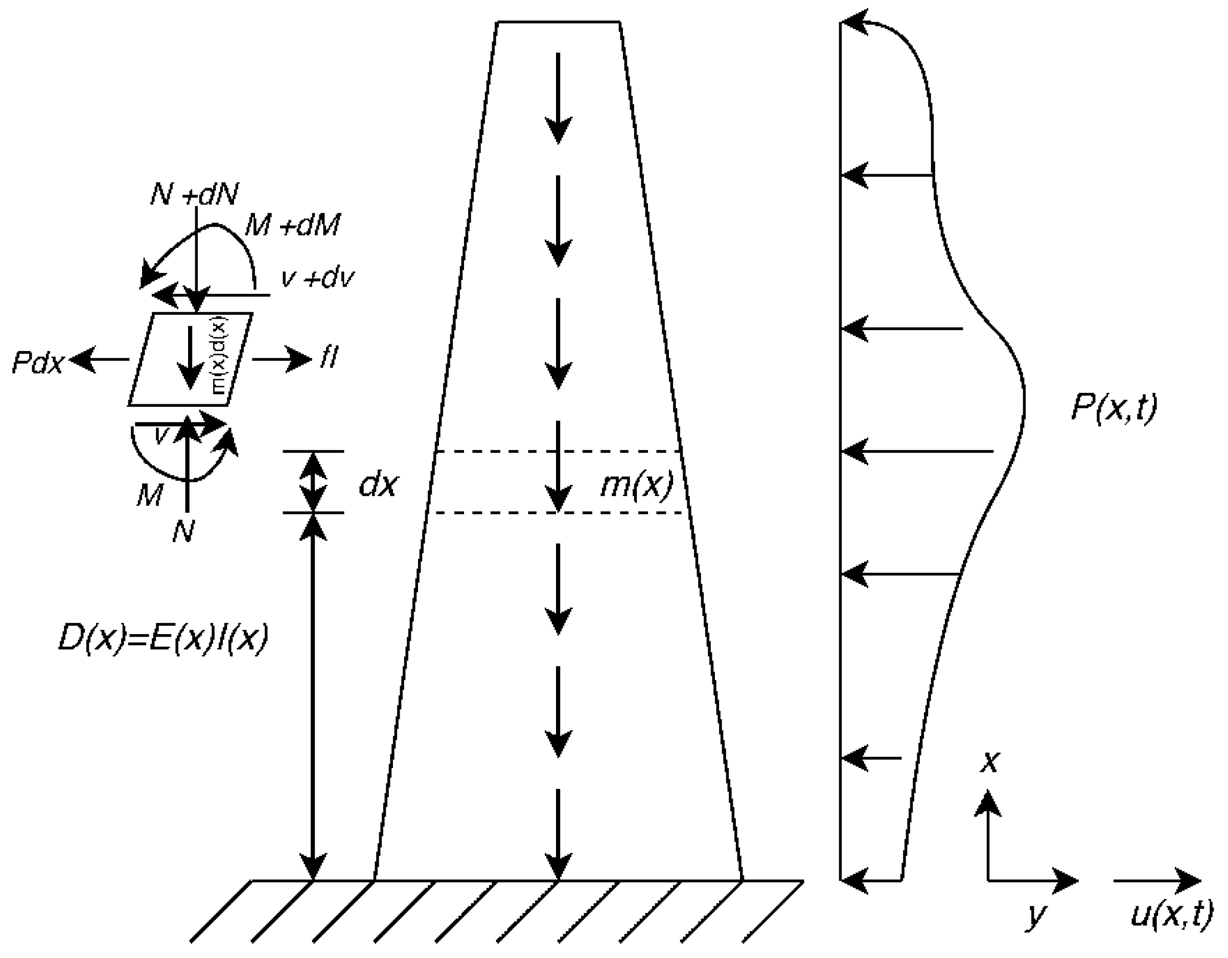
Figure 1 shows a straight-sided cantilever column without damping subjected to an external variable load, P. The governing equation for transverse vibration of this column can be written as:
where y is the lateral direction, x is the elevation from the base, u(x,t) is the motion of the column in y direction, m(x) is mass per unit length and P(x,t) is the external transverse force.
We know that:
where ν(x,t) is transverse shear, M(x,t) is the bending moment, ρ(x) is density and A(x) is the cross-sectional area. Substituting Equation (8) into Equation (7) gives:
where D(x) = E(x)I(x) is flexural rigidity, E(x) is Young’s modulus and I(x) is the area moment of inertia.
This is the general governing differential equation for vibration of a non-prismatic Bernoulli beam (column) under variable transverse force without considering damping. Setting P(x,t) = 0, the free vibration equation is obtained.
In the above system of equations, the deflection due to the shear stress in the column was ignored. The analysis of beam (column) vibration including both the effects of rotational inertia and shear deformation is called Timoshenko beam theory, which is outside the scope of this paper.
Considering the motion represented by harmonic vibration, the transverse motion of the column is obtained using the following relation:
where ϕ(x) and ω are the mode shape function and angular natural frequency of the beam, respectively. Substitution of Equation (10) into Equation (9) leads to:
For simplicity, for a column with a non-prismatic circular cross-section, we can define a non-dimensional coordinate ξ = x/L, then:
where α is the taper ratio [(D0-Dt)/D0] and D0 and Dt are the diameters of the tree at the base and top of the tree stem, respectively.
In general, we can rewrite the flexural rigidity and distributed mass as:
where I0, E0, ρ0 and A0 are the area moment of inertia, Young’s modulus, density and cross-section area at the base of the stem, respectively.
Consequently, Equation (11) can be transformed into a normalised form:
Therefore, we can define natural frequency parameter (λ) as:
The column base condition is bounded by two cases: clamped (fixed) and pinned. In general, we can consider intermediate cases using a rotational spring restraint at the base of the column. The deflection, u, is therefore related to the rotation angle, θ, by:
The boundary conditions applied to this column at the spring-supported end are:
where K is the rotational spring stiffness and the spring is assumed to be massless.
2.2. Calculation of Natural Frequency Using Numerical Analysis
The first natural frequency parameter (λ) of a column was found with the generalised eigenfrequency approach using the finite element analysis method. The commercial software SAP2000 (Computers and Structures Inc, Berkeley, CA, USA) and COMSOL Multiphysics (COMSOL Inc, Burlington, MA, USA) were used to investigate the effect of the different parameters on the natural frequency of non-prismatic circular columns. A free end–fixed base case was modelled, with rigid support for torsional moments and lateral translations. The column was discretised (sub-divided) into finite elements, with the properties varying linearly across the elements. The effect of variations in selected geometric and material properties on the vibration behaviour was investigated: column taper, end fixity, radial and longitudinal stiffness/density variation and relative crown mass and location.
2.2.1. Effect of Base Fixity
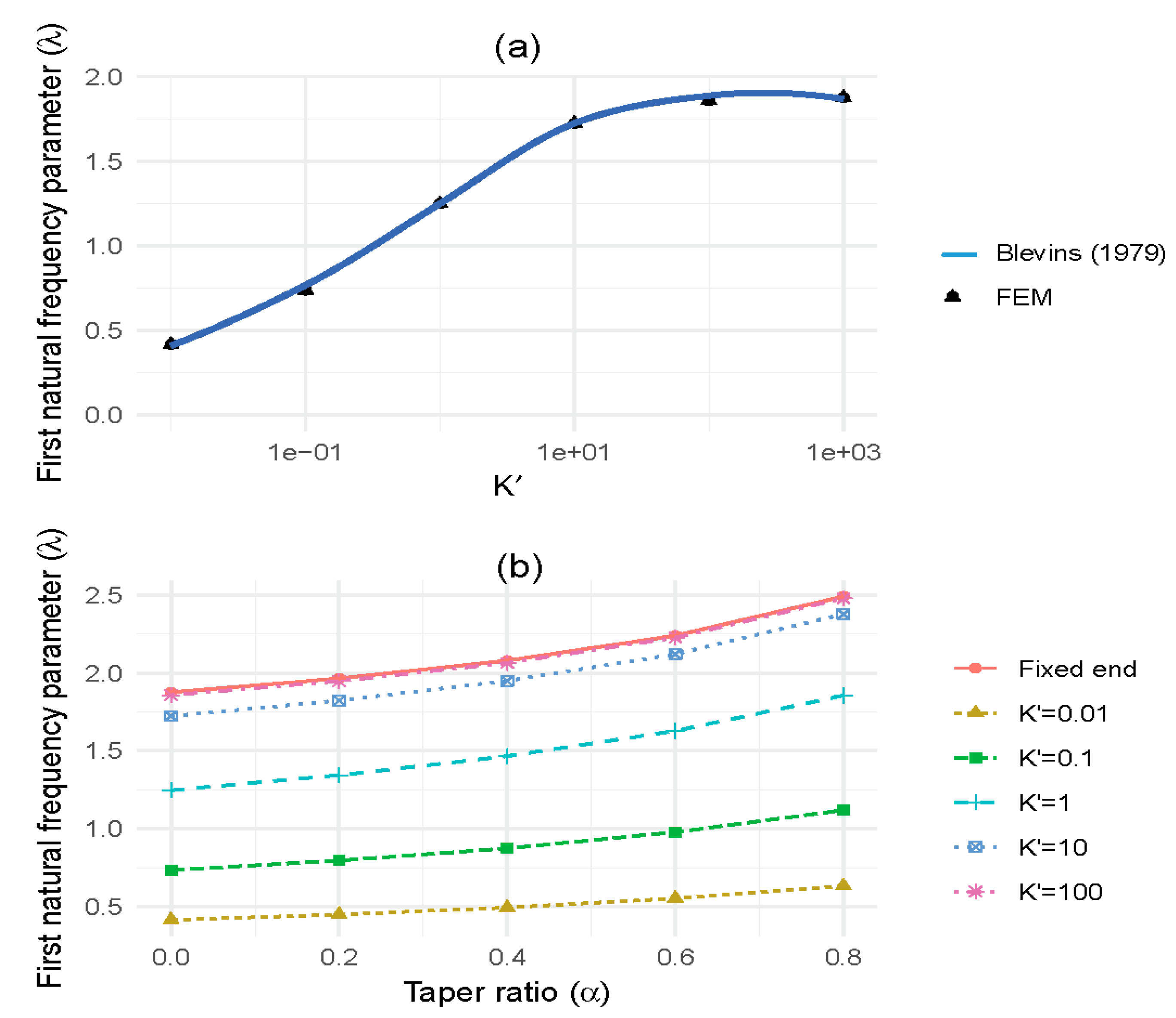
We did not attempt to model the behaviour of the whole root–soil system explicitly. Since the effect of the mass of the root–soil system on the overall behaviour has been found to be less significant with higher centres of mass of the above-ground components [18], this has been ignored. In addition, increases in the rooting depth will tend to increase the stiffness of the root–soil volume, counteracting any changes in the root–soil mass [47]. Hence, we have only included a basal rotational spring stiffness term (K) in the numerical models (assumed to be identical in the two orthogonal horizontal directions) to test the effect of the overall root–soil system rigidity on tree vibration behaviour. Each rotational stiffness was normalised by the stiffness magnitude to create a non-dimensional spring stiffness (K’) and the results are presented herein using the non-dimensional rotational stiffness K’ = KL/E0I0. The value of K’ will approach infinity for an equivalent clamped (fixed) case (θ0) and zero for a pinned condition (where M (base bending moment) 0). Validation of the models was conducted by comparison with the previous analyses of Blevins [30].
2.2.2. Effect of Longitudinal Stiffness Variation
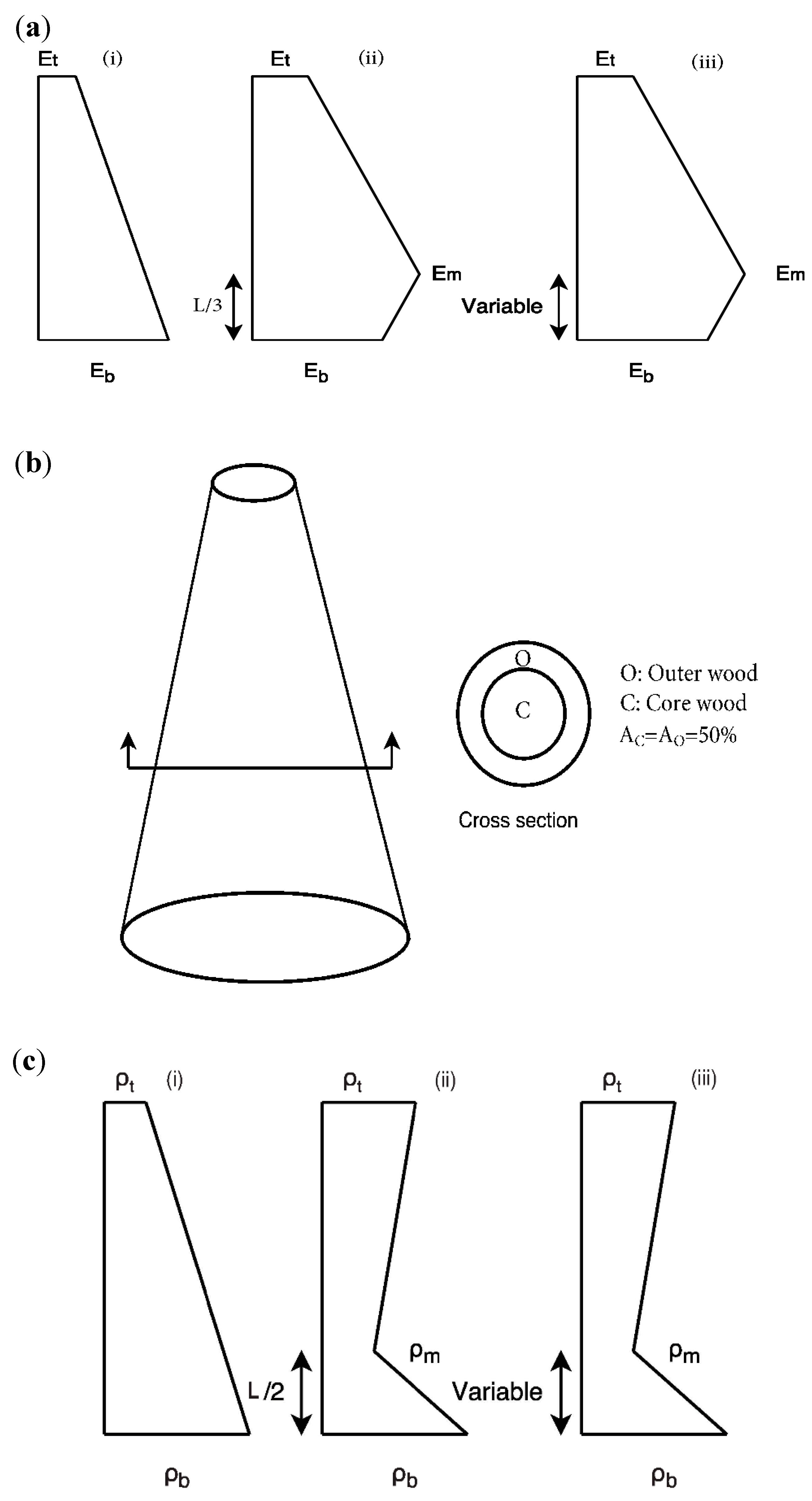
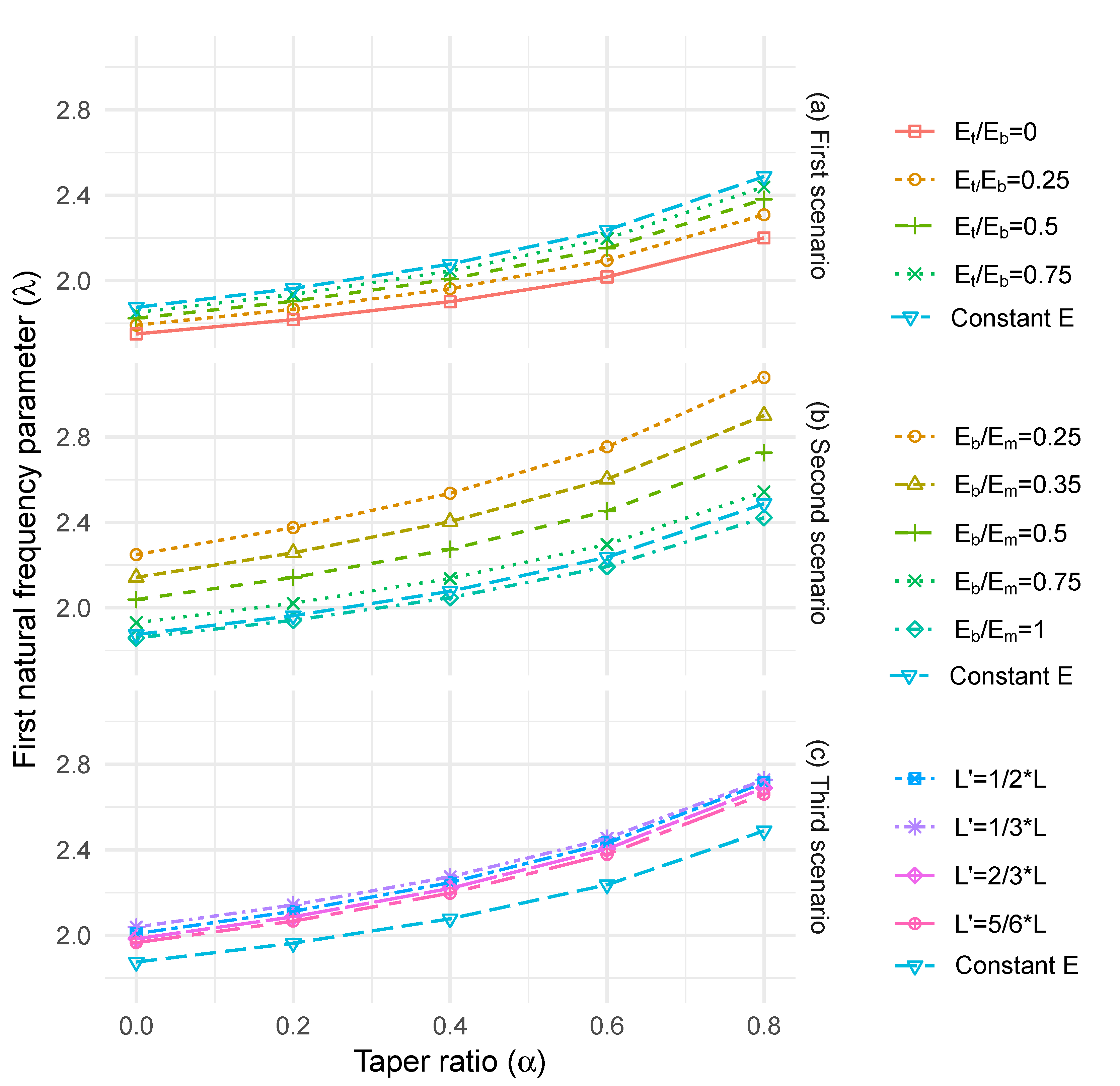
To model the longitudinal stiffness gradient variations for trees described in the literature, three cases (see Figure 2a, (i) to (iii)) were chosen for these analyses: (i) elastic modulus decreasing linearly from the bottom (Eb) to the top of the stem (Et), with Et/Eb = 0, 0.25, 0.5, 0.75 and 1, (ii) elastic modulus increasing linearly from the bottom (Eb) to one-third of the stem height (Em), followed by a linear decrease to the top of the stem (Et), with ϕ = 1/3, Et/Eb = 0.25 and Eb/Em = 0.25, 0.35, 0.5, 0.75 and 1 and (iii) Et/Eb = 0.25 and Eb/Em = 0.5 and varying the position of the gradient change (point m) with L/3, L/2, 2L/3 and 5L/6. In each case, the density (ρ) has been held constant, thus the value of E/ρ changes in a similar manner to that described in Equation (18).
2.2.3. Effect of Radial Stiffness Variation
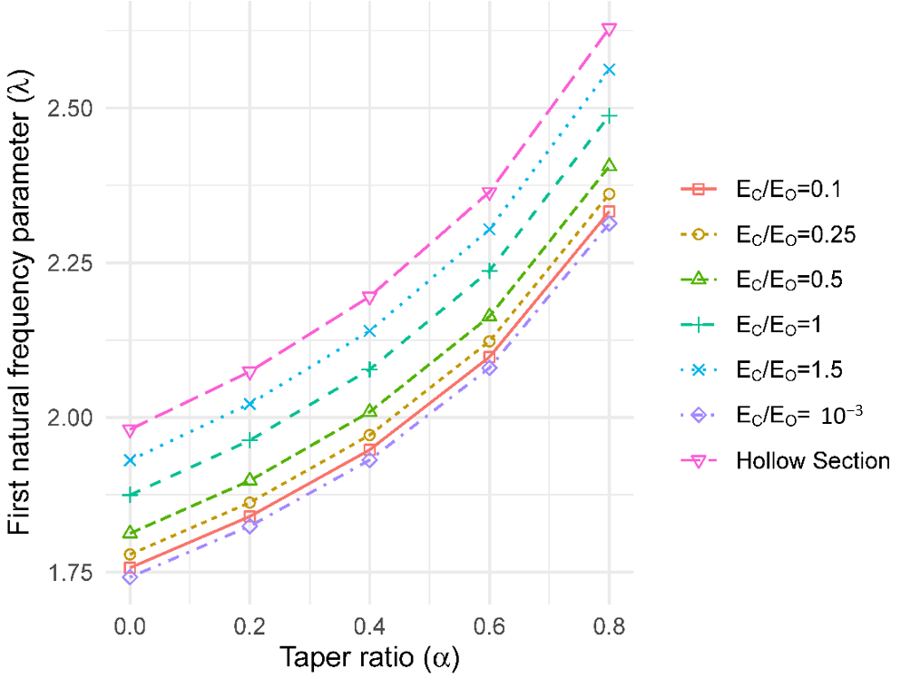
To consider the effect of radial stiffness (E) variation on the vibration behaviour, a composite section was defined with two concentric rings (see Figure 2b). Different stiffness moduli were assigned to each ring to represent the two different tree strategies (stiff core and stiff outer ring) outlined in the literature. The modelling herein assumes the presence of two rings of different radii, with the same area to represent the outer-wood and core-wood of the tree (i.e., Ao = Ac = 50% of the total area of the base cross-section). The stiffness of each ring was then varied according to the ratios: Ec/Eo of 10−3, 0.1, 0.25, 0.5, 1 and 1.5. The same density was assumed for both the outer-wood and core-wood. To calculate the values of first natural frequency parameter (λ), outer-wood properties at the base were used.
2.2.4. Effect of Longitudinal Density Variation
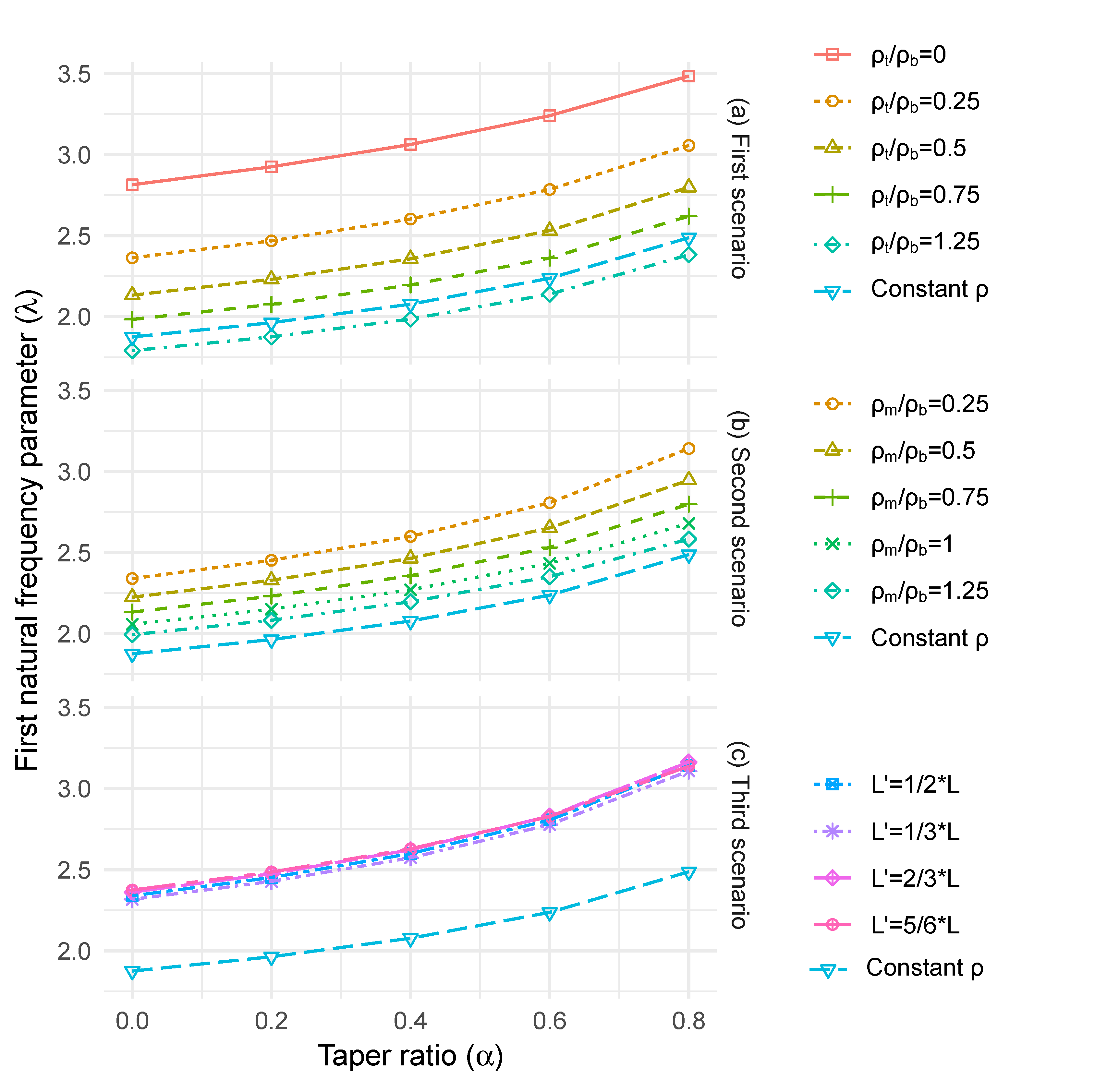
To model the longitudinal density gradients reported in the literature, three cases (see Figure 2c, (i) to (iii)) were chosen for analysis: (i) density varying linearly from the bottom (ρb) to the top of the stem (ρt), with ρt/ρb = 0, 0.25, 0.5, 0.75,1 and 1.25, (ii) density decreasing linearly from the bottom (ρb) to half of the stem height (ρm), followed by a linear increase to the top of the stem (ρt), with ϕ = 1/2, ρt/ρb = 0. 5 and ρm/ρb = 0.25, 0.5, 0.75, 1 and 1.25 and (iii) ρt/ρb = 0.5 and ρm/ρb = 0.25 and varying the position of the gradient change (point m) with L/3, L/2, 2L/3 and 5L/6. In each case, the stiffness (E) has been held constant, as shown in Equation (19).
2.2.5. Effect of Radial Density Variation
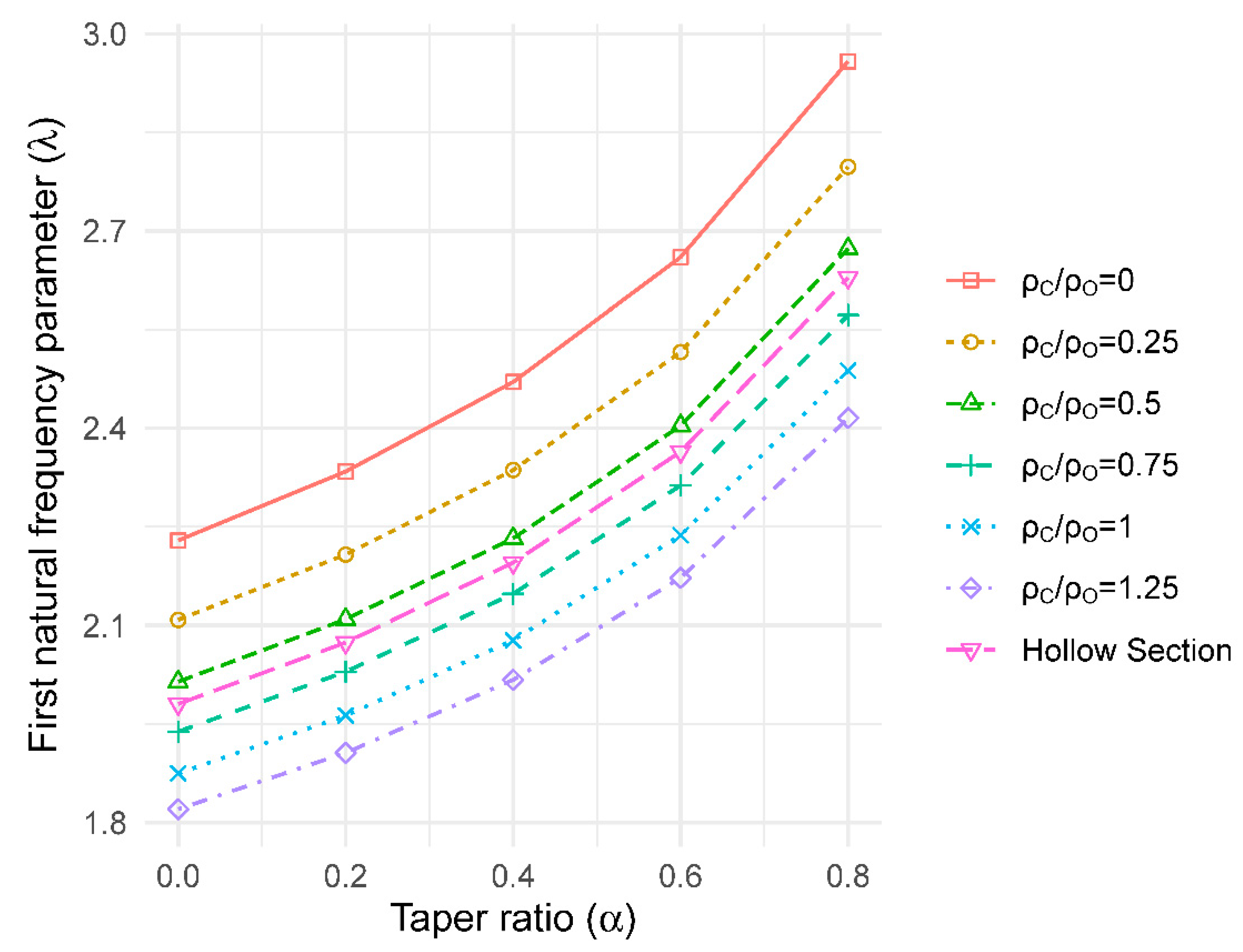
A similar approach to that used for radial stiffness variation was used to model the effect of radial density (ρ) variation on vibration behaviour. A composite section was defined with two concentric rings (see Figure 2b). Different densities were assigned to each ring to explore the two different strategies (light core and heavy outer ring) proposed in the literature. Two rings of different radii were defined, with the same area to represent the core-wood and outer-wood of the tree (i.e., Ao = Ac = 50% of the total area of the base cross-section). The density for each ring was then varied according to the ratios: ρc/ρo of 0, 0.25, 0.5, 1 and 1.25. The same elastic modulus was assumed for both the core-wood and outer-wood. To calculate the values of first natural frequency parameter (λ), outer-wood properties at the base were used.
2.2.6. Effect of Crown Mass
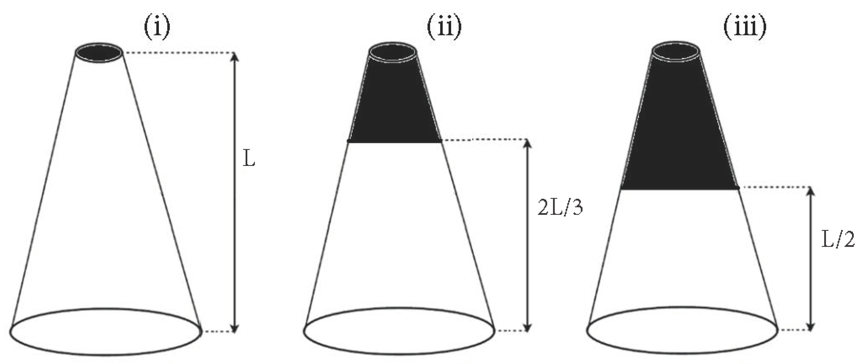
The effect of crown mass on the natural frequency was investigated by creating an equivalent “crown” using an additional mass (Wc) at different locations along the stem (see Figure 3). (i) In the first case, the additional crown mass was applied to the top of the stem, (ii) in the second, the same crown-to-stem mass ratios were applied to the upper two-thirds (by volume) of the stem and (iii) in the third case, they were applied to the upper half (by volume) of the stem. In all cases, we define different crown-to-stem mass ratios (Wc/Ws) at these particular locations.
2.3. Estimating Natural Frequency for Coniferous and Broadleaved Trees
Fundamental vibrational frequencies (fn) were collated from the literature on field studies of 703 broadleaf and conifer trees growing at different sites and under different conditions, spanning height and DBH ranges of 5.9–35.4 m and 6.9–82.8 cm, respectively [11,12,15,28,31,48,49,50,51,52,53]. These field data were used to validate the tapered cantilever beam model and provide further fundamental understanding of the sway behaviour of conifer and broadleaf trees. Results from these studies were used to estimate the natural frequencies and damping ratios of trees with the presence or absence of foliage, and for full and de-branched crowns, enabling the effects of the crown architecture to also be assessed. The field sway data covers thirteen different species: (a) conifers—Sitka spruce (Picea sitchensis), Douglas-fir (Pseudotsuga menziesii (Mirb.) Franco), Norway spruce (Picea abies), white spruce (Picea glauca (Moench) Voss.), Lodgepole pine (Pinus contorta Dougl.), Scots pine (Pinus sylvestris L.), Corsican pine (Pinus nigra Arnold) and red pine (Pinus resinosa Ait.), and (b) broadleaves—red maple (Acer rubrum L.), sugar maple (Acer saccharum Marsh.), shagbark hickory (Carya ovata (Mill) K. Koch), red oak (Quercus rubra L.) and lime (Tilia europaea L.). Data on the stiffness (E), density (ρ), taper (α) and crown/stem mass ratio (Wc/Ws) were found for each species in the literature and are summarised in Table 1 (see the Electronic Supplementary Material, Tables S1 and S2). While these properties can all vary substantially within a species due to genetic and environmental factors, we only had species-level average values as data for the individual trees were not available. Instead, we assumed that these properties were normally distributed with a standard deviation that was equal to 5% of the mean value. We then ran 100 simulations of the model to test the sensitivity to variations in these properties. The data were split into four groups for analysis: (1) conifers with full crowns, (2) broadleaves with full crowns, (3) debranched conifers and (4) leafless broadleaves. The natural frequency parameter (λ) was assumed to be 1.5, except for the case of conifers with their branches removed, when it was assumed to have a value of 2.5. Ordinary least squared regression was used to investigate the relationship between tree fundamental frequency and DBH/L2. This relationship was compared among the four analysis groups described above. Due to the limited overlap in values of DBH/L2 for several of the broadleaved species, it was not possible to test whether this relationship differed among species. The level of agreement between the predictions from the tapered cantilever beam model and the field observations of fundamental natural frequency for these groups was assessed using Lin’s concordance correlation coefficient [54,55].
3. Results
3.1. Effect of Base Fixity
The relationship between the first natural frequency parameter, λ, and the non-dimensional rotational stiffness, K’, for tapered (cylindrical) columns is found to be non-linear (Figure 4a). There is very little increase in natural frequency for large changes in rotational stiffness above a value of K’ = 10. However, once the non-dimensional rotational stiffness (K’) falls below 10, the natural frequency begins to drop rapidly. Comparison between our numerical modelling and Blevins’ solutions show differences of less than 1%. For columns with different rates of taper (α), the variation in first natural frequency parameter, λ, with the non-dimensional rotational stiffness, K’, is shown in Figure 4b. The non-dimensional rotational stiffness was varied from K’ = 0.01 (equivalent pinned condition) to 100 (approaching a clamped condition). For more tapered stems, basal rotational restraint had a greater effect on the natural frequency.
3.2. Effect of Longitudinal Stiffness Variation
For cylindrical columns with constant E, the first natural frequency parameter, λ, increased with increasing column taper ratio (α) (Figure 5a–c). With a linear decrease in E from the bottom to the top of the stem, the natural frequency parameter decreased compared with the case of constant E. The effect of this change in stiffness was relatively small for cylindrical columns (up to 7%), but more significant for highly tapered columns (up to 12%) (Figure 4a). This is due to the more rapid changes in stiffness compared to the sectional area. Under the assumption of a peak in stiffness at half stem height, the natural frequency increased relative to the uniform E case (up to 17%), with the greatest increase occurring for the more tapered stems (Figure 4b). Under the case of the varying changepoint height for E, the largest increases in natural frequency occurred at the lowest change point and for the most highly tapered stems. However, the magnitude of increase was very similar for all changepoint heights (up to 10%).
3.3. Effect of Radial Stiffness Variation
The value of the natural frequency parameter decreased with reducing stiffness ratio (i.e., outer-wood E > core-wood E), up to 7% for both cylindrical and tapered columns (Figure 6). According to the model results, the elastic ratio of 10−3 is a lower bound for the behaviour. Beyond this point, the behaviour of the stem approaches that of a hollow section. For the stiffness ratio of Ec/Eo = 1.5, an increase in the natural frequency of up to 3% was found.
3.4. Effect of Longitudinal Density Variation
For a cylindrical column with no taper, a reduction in density from the base to the top resulted in an increase in λ (up to 50%) (Figure 7a). The effect of this reduction in density on λ was less significant for highly tapered columns (up to 40%). This is due to the less rapid changes in mass compared to the sectional area. For the case of a change in density at the midpoint height of the column, the natural frequency increases (up to 23%), and this change was more evident for the highly tapered columns (Figure 7b). Even when the density at the midpoint height was greater than at the base, λ still increased as we assumed that density at the top of the column was 50% of the value at the base. For the case where the height of the minimum value varied up the column, the natural frequency increased, and the largest increase occurred with the highest change point (Figure 7c). However, the magnitude of the increase was very similar for all the changepoint heights (up to 27%).
3.5. Effect of Radial Density Variation
The value of the natural frequency parameter decreased with reducing ratio of core-wood density to outer-wood density ratio, for both cylindrical and tapered columns (Figure 8). According to the model results, the density ratio of 0 is an upper bound for the behaviour. This condition approaches that of a weightless core section.
3.6. Effect of Crown Mass
The natural frequency reduces as the relative crown weight increases (by up to 60%) (Figure 9). When there is no additional crown mass (i.e., Wc/Ws = 0), taper has a noticeable effect on the natural frequency parameter. However, as the ratio of crown mass to stem mass increases, the natural frequency becomes invariant to changes in taper, particularly when the crown mass is added at 2L/3 and L/2 (Figure 9b,c). This suggests that the crown weight is dominating the taper effect to some extent. However, adding a crown mass to the very top of a tapered column reduces the natural frequency while increased taper ratio in the absence of a crown mass increases natural frequency (Figure 9a).
3.7. Estimating Natural Frequency for Coniferous and Broadleaved Trees
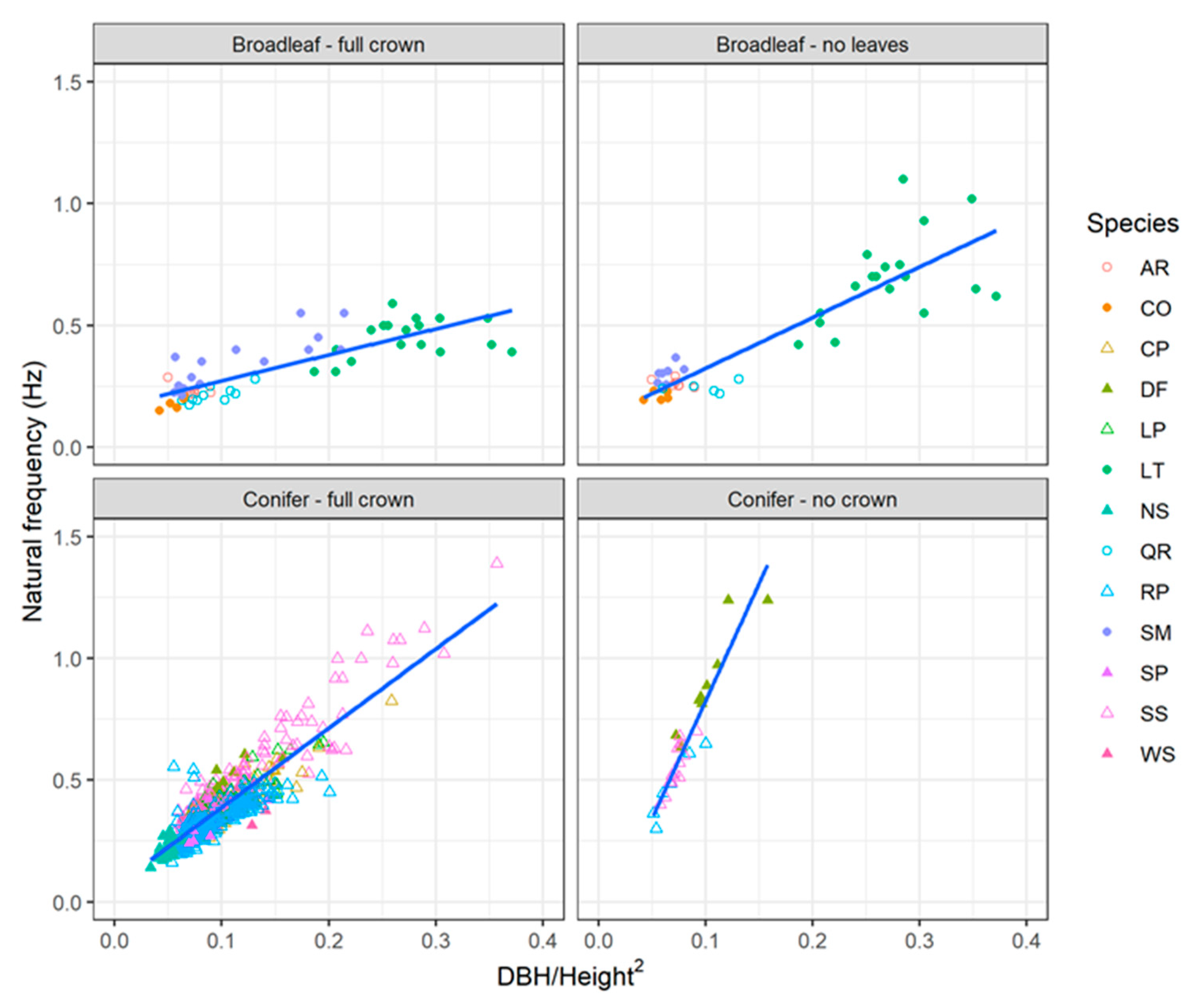
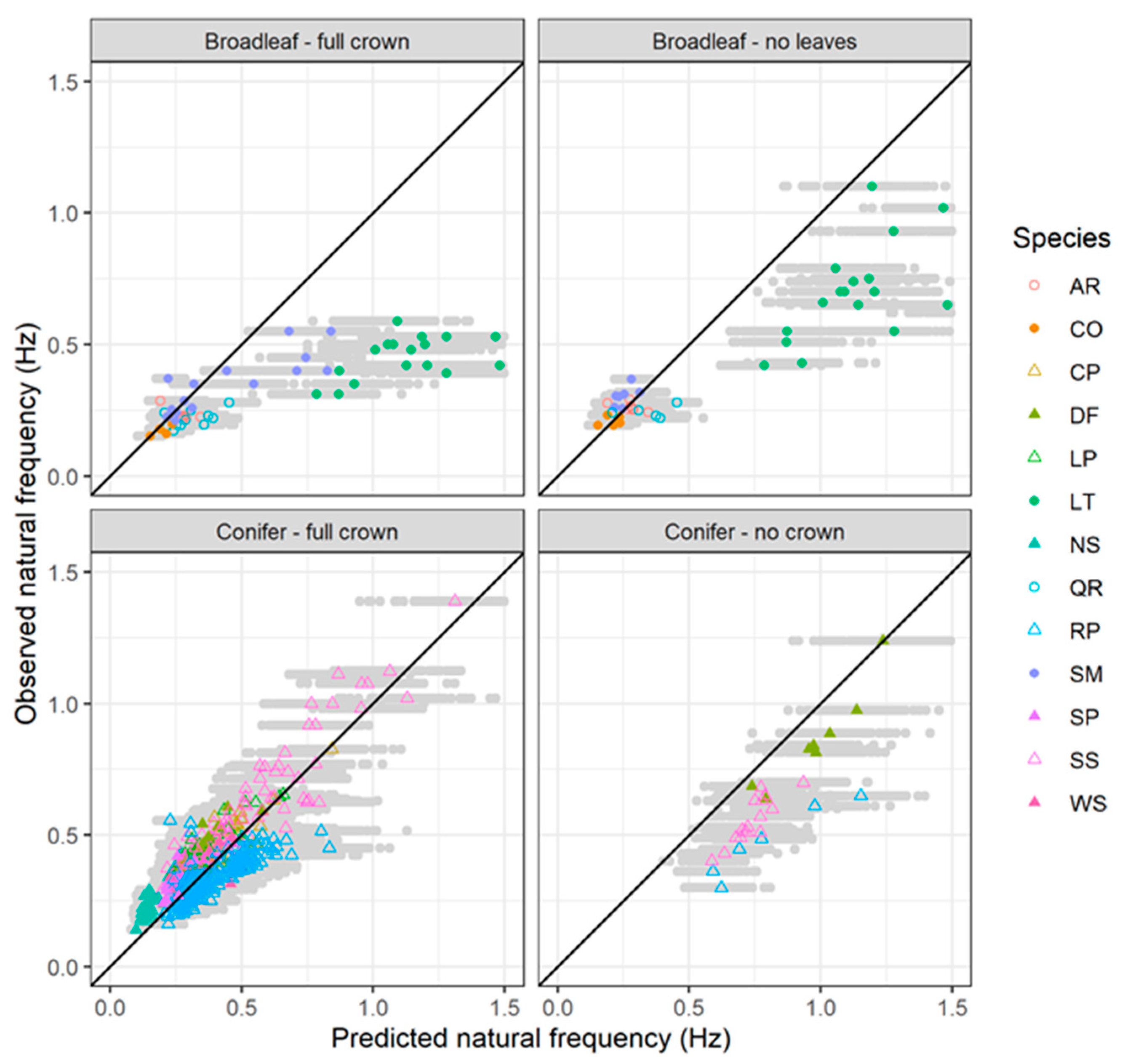
There was a strong relationship between tree natural frequency and the ratio of diameter at breast height to total tree height squared (Figure 10). However, the slope of this relationship differed significantly among the four different categories (p < 0.0001). The slope was lowest for broadleaved trees with full crown and was steepest for conifers with their branches removed. There was some indication that the relationship may be non-linear, especially for the broadleaved trees with full crown; however, this is mostly due to the dataset for lime trees which has several high leverage points (i.e., trees with high values of DBH/L2 and comparatively low natural frequency). The fundamental natural frequencies predicted by the model proposed in this paper were in general agreement with field observations for conifers with full crown (concordance correlation coefficient = 0.79) (Figure 11). The model overpredicted the natural frequencies of coniferous trees with their branches removed and had much poorer performance for broadleaved trees, particularly those with full crown (concordance correlation coefficient < 0.3). This latter result was mostly driven by the dataset for lime trees where there was a weak relationship between tree natural frequency and DBH/L2. With the exception of these data, all the simulations produced results that were in general agreement with field observations.
4. Discussion
As well as the stem geometry and material properties, the crown and branch architecture has been shown to influence the sway frequency, damping and dynamic amplification factor of trees under dynamic loading [15,22,25,32]. The crown shape of trees can vary according to the species and is due to a combination of the inherent form and their growth environment. McCurdy el al. [56] identified six distinct crown shapes: oblong, round, oval, vase, pyramidal and weeping. In forest settings, crown shape is often influenced by tree position relative to other trees in the canopy (although the basic shape is characteristic for all species). The primary factor determining these characteristic crown shapes is apical (epinastic) dominance (i.e., the upward growth of a leader at the expense of the lateral shoots) [57]. Tree species with strong apical dominance usually have height to width dominance and a single dominating trunk and leader. Examples of tree species of this type are sweet gum (Liquidambar styraciflua L.), Yellow tulip poplar (Liriodendron tulipifera L.), cottonwoods (Populus section Aigeiros), alders (Alnus spp.) and most conifers. These are termed excurrent crowns and favour oblong and pyramidal shapes [58]. In contrast, decurrent trees with weak apical dominance have crown widths that grow nearly as fast as their height (especially when open-grown) and this creates large spreading crowns. These species tend to have no predominant leader and can have similar multiple forks in the central trunk. These trees have crowns that tend to favour round or oval shapes and typical species are broadleaf trees such as oaks (Quercus spp.) and maples (Acer spp.) [58].
The tapered cantilever beam sway model proposed in this study adequately predicts the natural frequency for conifers, but not for broadleaves. As other researchers have found, excurrent trees have natural frequencies which are proportional to the product of DBH/L2 [11,32]. Interestingly, the presence of a crown seems to reduce the natural frequency and improves the fit of the model compared with the situation where the model is applied to a stem with the crown removed. Broadleaves tend to have a more complex geometry, with multiple close natural frequencies and are therefore more dependent on the branch/crown architecture and presence of leaves [17,32,53]. For the broadleaves with crowns, the model fit is generally quite poor, and as would be anticipated, this improves with the removal of the leaf mass. As occurs with excurrent trees, the natural frequency of decurrent trees also reduces with the removal of the leaf mass from the crown, although this change is relatively small compared to that for excurrent trees. These findings are supported by field studies [8,11,15,28], where pruning and seasonal changes have more profound effects on excurrent trees. The change in natural frequency with pruning have mostly been associated with mass change, but numerical studies by Kerzenmacher and Gardiner [19] showed that mass change alone could not completely account for the change in natural frequency, as trees went from a fully-branched state to a de-branched state. They hypothesized that branch swaying also had an effect on overall dynamic behaviour of trees.
In decurrent trees, the branch sway has much greater importance with relation to the natural frequency [53], leading to the divergence from the proposed mechanical sway model. The distribution of mass in conifers is also quite different, with a greater proportion of mass in the upper half of the crown, compared to broadleaves with a more distributed branch mass. Broadleaves may also have what is known as multiple resonance damping [17,24]. Transfer of mechanical energy can occur due to the overlap of the resonance spectra of the large branch structures, which increases the structural damping. The frequency of these large branches can be close to the natural frequency of the entire tree and the action of the primary and higher-order branches therefore combine to produce the overall sway response [59,60,61]. The energy exchange between these different branches is related to their amplitudes, frequencies and the phase relations, and this creates a coupled damped oscillation system with characteristics very different from the proposed tapered cantilever beam model. It may be feasible that the simpler pendulum response and crown architecture of excurrent trees may make them more vulnerable to dynamic wind damage and higher wind-induced forces.
Previous studies modelling tree dynamic behaviour have generally assumed uniform wood properties in both the radial and longitudinal directions [19,25,50]. However, this ignores the typical patterns that are observed in practice. In many wood science studies, radial and longitudinal patterns of wood density and stiffness are measured, typically at a standard moisture content [33,43,44,45]. In standing trees, these gradients may differ due to moisture content differences between sapwood and heartwood. In our simulations, we accounted for both moisture content differences and gradients in wood properties through varying the ratio of core-wood and outer-wood properties and incorporating different longitudinal gradients. These encompassed the full range of patterns that are expected to exist in nature. Our results showed that varying the internal wood properties’ distributions has a significant effect on tree dynamic behaviour. As expected, placing the stiffer material on the periphery of the stem increases natural frequency as this material is located further from the neutral axis of the stem. While the application of the model to predict natural frequencies of conifers and broadleaves trees used published values of wood density and modulus of elasticity from wood science literature, there is large variation in these properties among individuals within a species and across geographical gradients [45,62,63]. Differences in values of density-specific stiffness (E/ρ) may explain some of the differences between observed and predicted fundamental natural frequencies.
The proposed model also enabled the effect of base fixity on natural frequency to be accounted for. Previous studies that have used the equations of motion for a taper cantilever beam as the basis to study tree oscillations have either assumed the tree to be rigidly anchored and adjusted the effective stem stiffness or represented the whole root–stem system as a spring with a given rotational stiffness. This is because there is a significant body of study is available for the vibration analysis of fixed base-free end columns. Much less work has been done on columns with reduced basal rotational restraint. This is a situation encountered in civil engineering for columns connecting to foundations with relatively ‘soft’ bases and electro-mechanics where nanostructures are fixed to elastic substrates. This problem has been modelled by introducing rotational spring restraint in place of the fixed (clamped) column base condition. For trees, this represents a scenario where the rotational restraint of the root plate is relatively low, e.g., from loss of soil, reduced soil strength/stiffness or root damage [64]. The effect of changing the root system stiffness may be approximately assessed by inspection of the classical equation for rotational stiffness (K) of a rigid circular plate located on the surface of an elastic half-space [65]:
where G is the composite shear modulus of the soil and roots, R is the radius of the root plate and ν is the Poisson’s ratio of the soil and roots. This model is often applied to foundation problems, but in the current case, G and ν are related to the composite behaviour of the soil and roots in the root plate. This suggests that quite significant changes in soil packing (density) or moisture content are required for the rotational root plate stiffness to affect the vibration behaviour, particularly for trees with high taper ratios.
Overall, the modelling approach employed here has enabled the relative effect of variation in tree taper, internal wood properties, crown mass distribution and the base fixity on tree dynamic behaviour to be investigated. It provides an important advancement over earlier models that make much simpler assumptions for these factors and enables the various biomechanical strategies employed by trees to be investigated. Although the proposed model appears to predict the behaviour of conifers adequately, modelling the mechanical behaviour of broadleaved trees can still be undertaken using the finite element method, but will require a more detailed description of the tree topology. New technologies such as terrestrial laser scanning systems provide a means for capturing the data required to generate realistic descriptions of tree architecture and the resulting mass and stiffness distributions needed to predict their dynamic behaviour [32].
5. Conclusions
Finite element-based vibration analysis was used to investigate the behaviour of free end–fixed base columns. A non-prismatic elastic circular column of height L was analysed, taking self-weight into account. Various scenarios were considered: column taper, base fixity, stiffness (E) and density (ρ) variation along the height and cross-section, and crown mass. The effect on the sway natural frequency was assessed in each case. Validation against benchmark problems was conducted satisfactorily. The results indicate that column taper, base fixity, ellipticity and E/ρ ratio are particularly important for this problem. Comparison with published literature results from actual field-based tree swaying tests shows that the model is able to adequately represent the behaviour of conifer trees but is less suited to broadleaved trees with their more complex architecture. Due to the simple presentation, use of the results contained in the paper should improve estimates of natural frequency for trees and allow more subtle characterisation and understanding of the problem.
Supplementary Materials
The following are available online at https://0-www-mdpi-com.brum.beds.ac.uk/1999-4907/11/9/915/s1: Supplement 1: Sources of information on wood properties, tree mass and taper values used to predict tree sway frequencies (Tables S1 and S2).
Author Contributions
Conceptualisation, T.N.; methodology, M.D. and T.N.; formal analysis, T.N., M.D. and J.R.M.; visualisation, M.D. and J.R.M.; writing—original draft preparation, M.D.; writing—review and editing, J.R.M. and T.N.; supervision, T.N. All authors have read and agreed to the published version of the manuscript.
Funding
The authors would like to acknowledge the financial support of Natural Sciences and Engineering Research Council (Grant No.: RGPIN-2015-06062).
Conflicts of Interest
The authors declare no conflict of interest. The funders had no role in the design of the study; in the collection, analyses, or interpretation of data; in the writing of the manuscript, or in the decision to publish the results.
References
- De Langre, E. Effects of wind on plants. Annu. Rev. Fluid Mech. 2008, 40, 141–168. [Google Scholar] [CrossRef] [Green Version]
- Gardiner, B.; Berry, P.; Moulia, B. Review: Wind impacts on plant growth, mechanics and damage. Plant Sci. 2016, 245, 94–118. [Google Scholar] [CrossRef] [PubMed]
- Moore, J.; Gardiner, B.; Sellier, D. Tree Mechanics and Wind Loading. In Plant Biomechanics; Geitmann, A., Gril, J., Eds.; Springer International Publishing: Cham, Switzerland, 2018; pp. 79–106. ISBN 978-3-319-79098-5. [Google Scholar]
- Grace, J. Plant Response to Wind; Academic Press: London, UK, 1977. [Google Scholar]
- Telewski, F.W. Wind-induced physiological and developmental responses in trees. In Wind and Trees; Coutts, M.P., Grace, J., Eds.; Cambridge University Press: Cambridge, UK, 1995; pp. 237–263. [Google Scholar]
- Moulia, B.; Coutand, C.; Julien, J.-L. Mechanosensitive control of plant growth: Bearing the load, sensing, transducing, and responding. Front. Plant Sci. 2015, 6, 52. [Google Scholar] [CrossRef] [PubMed]
- Fournier, M.; Dlouhá, J.; Jaouen, G.; Almeras, T. Integrative biomechanics for tree ecology: Beyond wood density and strength. J. Exp. Bot. 2013, 64, 4793–4815. [Google Scholar] [CrossRef] [PubMed] [Green Version]
- Gardiner, B.A. Mathematical modelling of the static and dynamic characteristics of plantation trees. In Mathematical Modelling of Forest Ecosystems; Franke, J., Roeder, A., Eds.; Sauerlander’s Verlag: Frankfurt am Main, Germany, 1992; pp. 40–61. [Google Scholar]
- Gardiner, B.; Peltola, H.; Kellomäki, S. Comparison of two models for predicting the critical wind speeds required to damage coniferous trees. Ecol. Model. 2000, 129, 1–23. [Google Scholar] [CrossRef]
- Mayer, H. Wind-induced tree sways. Trees 1987, 1, 195–206. [Google Scholar] [CrossRef]
- Moore, J.R.; Maguire, D.A. Natural sway frequencies and damping ratios of trees: Concepts, review and synthesis of previous studies. Trees-Struct. Funct. 2004, 18, 195–203. [Google Scholar] [CrossRef]
- Jonsson, M.J.; Foetzki, A.; Kalberer, M.; Lundström, T.; Ammann, W.; Stöckli, V. Natural frequencies and damping ratios of Norway spruce (Picea abies (L.) Karst) growing on subalpine forested slopes. Trees 2007, 21, 541–548. [Google Scholar] [CrossRef]
- Blackwell, P.G.; Rennolls, K.; Coutts, M.P. A root anchorage model for shallowly rooted Sitka spruce. Forestry 1990, 63, 73–91. [Google Scholar] [CrossRef]
- Baker, C.J. Measurements of the natural frequencies of trees. J. Exp. Bot. 1997, 48, 1125–1132. [Google Scholar] [CrossRef]
- Moore, J.R.; Maguire, D.A. Natural sway frequencies and damping ratios of trees: Influence of crown structure. Trees 2005, 19, 363–373. [Google Scholar] [CrossRef]
- James, K.R.; Haritos, N.; Ades, P.K. Mechanical stability of trees under dynamic loads. Am. J. Bot. 2006, 93, 1522–1530. [Google Scholar] [CrossRef] [PubMed]
- Kane, B.; James, K.R. Dynamic properties of open-grown deciduous trees. Can. J. For. Res. 2011, 41, 321–330. [Google Scholar] [CrossRef]
- Horvath, E.; Sitkei, G. Energy consumption of selected tree shakers under different operational condition. J. Agric. Eng. Res. 2001, 80, 191–199. [Google Scholar] [CrossRef]
- Kerzenmacher, T.; Gardiner, B. A mathematical model to describe the dynamic response of a spruce tree to the wind. Trees 1998, 12, 385. [Google Scholar] [CrossRef]
- Saunderson, S.E.T.; England, A.H.; Baker, C.J. A Dynamic Model of the Behaviour of Sitka Spruce in High Winds. J. Theor. Biol. 1999, 200, 249–259. [Google Scholar] [CrossRef] [PubMed]
- Sellier, D.; Fourcaud, T. A mechanical analysis of the relationship between free oscillations of Pinus pinaster Ait. saplings and their aerial architecture. J. Exp. Bot. 2005, 56, 1563–1573. [Google Scholar] [CrossRef] [Green Version]
- Sellier, D.; Fourcaud, T.; Lac, P. A finite element model for investigating effects of aerial architecture on tree oscillations. Tree Physiol. 2006, 26, 799–806. [Google Scholar] [CrossRef] [Green Version]
- Sellier, D.; Brunet, Y.; Fourcaud, T. A numerical model of tree aerodynamic response to a turbulent airflow. Forestry 2008, 81, 279–297. [Google Scholar] [CrossRef] [Green Version]
- Spatz, H.-C.; Bruchert, F.; Pfisterer, J. Multiple resonance damping or how do trees escape dangerously large oscillations? Am. J. Bot. 2007, 94, 1603–1611. [Google Scholar] [CrossRef]
- Moore, J.R.; Maguire, D.A. Simulating the dynamic behavior of Douglas-fir trees under applied loads by the finite element method. Tree Physiol. 2008, 28, 75–83. [Google Scholar] [CrossRef] [PubMed]
- Rodriguez, M.; de Langre, E.; Moulia, B. A scaling law for the effects of architecture and allometry on tree vibration modes suggests a biological tuning to modal compartmentalization. Am. J. Bot. 2008, 95, 1523–1537. [Google Scholar] [CrossRef] [PubMed]
- Spatz, H.-C.; Speck, O. Oscillation frequencies of tapered plant stems. Am. J. Bot. 2002, 89, 1–11. [Google Scholar] [CrossRef] [PubMed] [Green Version]
- Milne, R. Dynamics of swaying of Picea sitchensis. Tree Physiol. 1991, 9, 383–399. [Google Scholar] [CrossRef]
- Humar, J.L. Dynamics of Structures, 3rd ed.; CRC Press-Taylor & Francis Croup: Boca Raton, FL, USA, 2012; ISBN 978-0-415-62086-4. [Google Scholar]
- Blevins, R.D. Formulas for Natural Frequency and Mode Shape; Van Nostrand Reinhold Co.: New York, NY, USA, 1979; ISBN 978-0-442-20710-6. [Google Scholar]
- Mayhead, G.J. Sway periods of forest trees. Scott. For. 1973, 27, 19–23. [Google Scholar]
- Jackson, T.; Shenkin, A.; Moore, J.; Bunce, A.; van Emmerik, T.; Kane, B.; Burcham, D.; James, K.; Selker, J.; Calders, K.; et al. An architectural understanding of natural sway frequencies in trees. J. R. Soc. Interface 2019, 16, 20190116. [Google Scholar] [CrossRef] [Green Version]
- Lachenbruch, B.; Moore, J.R.; Evans, R. Radial Variation in Wood Structure and Function in Woody Plants, and Hypotheses for Its Occurrence. In Size- and Age-Related Changes in Tree Structure and Function; Tree, Physiology; Meinzer, F.C., Lachenbruch, B., Dawson, T.E., Eds.; Springer: Dordrecht, The Netherlands, 2011; Volume 4, pp. 121–164. ISBN 978-94-007-1241-6. [Google Scholar]
- Niklas, K.J. Plant Biomechanics: An Engineering Approach to Plant Form and Function; University of Chicago Press: Chicago, IL, USA, 1992; ISBN 978-0-226-58630-4. [Google Scholar]
- Niklas, K. Mechanical properties of black locust (Robinia pseudoacacia L.) wood. Size- and age-dependent variations in sap- and heartwood. Ann. Bot. 1997, 79, 265–272. [Google Scholar] [CrossRef] [Green Version]
- Koch, P. Utilization of Hardwoods Growing on Southern Pine Sites-Volume 1; USDA-Forest Service, Southern Forest Experiment Station: Asheville, NC, USA, 1985.
- Rich, P.M. Mechanical structure of the stem of arborescent palms. Bot. Gaz. 1987, 148, 42–50. [Google Scholar] [CrossRef] [Green Version]
- Wiemann, M.C.; Williamson, G.B. Wood specific gravity gradients in tropical dry and montane rain forest trees. Am. J. Bot. 1989, 76, 924–928. [Google Scholar] [CrossRef]
- Xu, P.; Walker, J.C.F. Stiffness gradients in radiata pine trees. Wood Sci. Technol. 2004, 38, 1–9. [Google Scholar] [CrossRef]
- Waghorn, M.J.; Mason, E.G.; Watt, M.S. Influence of initial stand density and genotype on longitudinal variation in modulus of elasticity for 17-year-old Pinus radiata. Forest Ecol. Manag. 2007, 252, 67–72. [Google Scholar] [CrossRef]
- Hirakawa, Y.; Fujisawa, Y. The S2 microfibril angle variations in the vertical direction of latewood tracheids in sugi (Cryptomeria japonica) trees. Mokuzai Gakkaishi/J. Jpn. Wood Res. Soc. 1996, 42, 107–114. [Google Scholar]
- Perstorper, M. Lengthwise variation in grading parameters and comparison with bending strength tests. In Proceedings of the 10th International Symposium on Nondestructive Testing of Wood; Santoz, J.L., Ed.; Presses Polytechniques et Universitaires Romandes: Lausanne, Switzerland, 1996; pp. 341–350. [Google Scholar]
- Gardiner, B.; Leban, J.-M.; Auty, D.; Simpson, H. Models for predicting wood density of British-grown Sitka spruce. Forestry 2011, 84, 119–132. [Google Scholar] [CrossRef]
- Auty, D.; Achim, A.; Macdonald, E.; Cameron, A.D.; Gardiner, B.A. Models for predicting wood density variation in Scots pine. Forestry 2014, 87, 449–458. [Google Scholar] [CrossRef] [Green Version]
- Kimberley, M.O.; Cown, D.J.; McKinley, R.B.; Moore, J.R.; Dowling, L.J. Modelling variation in wood density within and among trees in stands of New Zealand-grown radiata pine. N. Z. J. For. Sci. 2015, 45, 22. [Google Scholar] [CrossRef] [Green Version]
- ght loading. For. Int. J. For. Res. 2019, 92, 393–405. [CrossRef]
- Hushmand, B. Experimental Studies of Dynamic Response of Foundations. Ph.D. Thesis, California Institute of Technology, Pasadena, CA, USA, 1983. [Google Scholar]
- Gardiner, B.A.; Stacey, G.R.; Belcher, R.E.; Wood, C.J. Field and wind tunnel assessments of the implications of respacing and thinning for tree stability. Forestry 1997, 70, 233–252. [Google Scholar] [CrossRef]
- Bunce, A.; Volin, J.C.; Miller, D.R.; Parent, J.; Rudnicki, M. Determinants of tree sway frequency in temperate deciduous forests of the Northeast United States. Agric. For. Meteorol. 2019, 266, 87–96. [Google Scholar] [CrossRef] [Green Version]
- Flesch, T.K.; Wilson, J.D. Wind and remnant tree sway in forest cutblocks. II. Relating measured tree sway to wind statistics. Agric. For. Meteorol. 1999, 93, 243–258. [Google Scholar] [CrossRef] [Green Version]
- Webb, V.A.; Rudnicki, M.; Muppa, S.K. Analysis of tree sway and crown collisions for managed Pinus resinosa in southern Maine. For. Ecol. Manag. 2013, 302, 193–199. [Google Scholar] [CrossRef]
- Sugden, M.J. Tree sway period—A possible new parameter for crown classification and stand competition. For. Chron. 1962, 38, 336–344. [Google Scholar] [CrossRef]
- Kane, B.; Modarres-Sadeghi, Y.; James, K.R.; Reiland, M. Effects of crown structure on the sway characteristics of large decurrent trees. Trees 2014, 28, 151–159. [Google Scholar] [CrossRef]
- Lin, L.I.-K. A Concordance Correlation Coefficient to Evaluate Reproducibility. Biometrics 1989, 45, 255. [Google Scholar] [CrossRef] [PubMed]
- Lin, L.I.-K. A note on the concordance correlation coefficient. Biometrics 2000, 56, 324–325. [Google Scholar] [CrossRef]
- McCurdy, D.R.; Spangenberg, W.G.; Doty, C.P. How to Choose Your Tree: A Guide to Parklike Landscaping in Illinois, Indiana, and Ohio; Southern Illinois University Press: Carbondale, IL, USA, 1972; ISBN 978-0-8093-0514-8. [Google Scholar]
- Cline, M.G. Apical dominance. Bot. Rev. 1991, 57, 318–358. [Google Scholar] [CrossRef]
- Ford, E.D. Branching, crown structure and the control of timber production. In Attributes of Trees as Crop Plants; Cannell, M.G.R., Jackson, J.E., Eds.; Institute of Terrestrial Ecology: Huntingdon, UK, 1985; pp. 228–252. [Google Scholar]
- Scannell, B. Quantification of the Interactive Motions of the Atmospheric Surface Layer and a Conifer Canopy. Ph.D. Thesis, Cranfield Institute of Technology, Bedford, UK, 1983. [Google Scholar]
- Moore, J.R. Mechanical Behavior of Coniferous Trees Subjected to Wind Loading. Ph.D. Thesis, Oregon State University, Corvallis, OR, USA, 2002. [Google Scholar]
- Ciftci, C.; Brena, S.F.; Kane, B.; Arwade, S.R. The effect of crown architecture on dynamic amplification factor of an open-grown sugar maple (Acer saccharum L.). Trees 2013, 27, 1175–1189. [Google Scholar] [CrossRef]
- Antony, F.; Jordan, L.; Schimleck, L.R.; Clark, A.; Souter, R.A.; Daniels, R.F. Regional variation in wood modulus of elasticity (stiffness) and modulus of rupture (strength) of planted loblolly pine in the United States. Can. J. For. Res. 2011, 41, 1522–1533. [Google Scholar] [CrossRef]
- Kimberley, M.O.; Moore, J.R.; Dungey, H.S. Modelling the effects of genetic improvement on radiata pine wood density. N. Z. J. For. Sci. 2016, 46, 8. [Google Scholar] [CrossRef] [Green Version]
- Neild, S.A.; Wood, C.J. Estimating stem and root-anchorage flexibility in trees. Tree Physiol. 1999, 19, 141–151. [Google Scholar] [CrossRef]
- Borowicka, H. Uber ausmittig belaste starre Platten auf elastischisotorpem Untergrund. Ing. Arch. Berl. 1943, 1, 1–8. [Google Scholar]
Figure 1.
Schematic cantilever column without damping subjected to an external variable load.

Figure 2.
(a) Schematic of longitudinal stiffness variation scenarios (i) to (iii), (b) schematic of radial stiffness variation scenarios and (c) schematic of longitudinal density variation scenarios (i) to (iii).
Figure 2.
(a) Schematic of longitudinal stiffness variation scenarios (i) to (iii), (b) schematic of radial stiffness variation scenarios and (c) schematic of longitudinal density variation scenarios (i) to (iii).

Figure 3.
Schematic of crown mass location scenarios.

Figure 4.
(a) Comparison of theoretical and numerical first natural frequency parameter ratio with relative rotational base stiffness, and (b) taper ratio versus first natural frequency parameter ratio with varying rotational base stiffness.
Figure 4.
(a) Comparison of theoretical and numerical first natural frequency parameter ratio with relative rotational base stiffness, and (b) taper ratio versus first natural frequency parameter ratio with varying rotational base stiffness.

Figure 5.
(a) Taper ratio versus first natural frequency parameter ratio with longitudinal stiffness variation linearly from the bottom to the top end of the tree (first scenario), (b) taper ratio versus first natural frequency parameter ratio with longitudinal stiffness variation linearly from the bottom to one-third of the tree height, followed by a linear variation till the top end of the tree (second scenario) and (c) taper ratio versus first natural frequency parameter ratio with longitudinal stiffness variation linearly from the bottom to L’, followed by a linear variation till the top end of the tree (third scenario).

Figure 6.
Taper ratio versus first natural frequency parameter ratio with radial stiffness variation.
Figure 6.
Taper ratio versus first natural frequency parameter ratio with radial stiffness variation.

Figure 7.
(a) taper ratio versus first natural frequency parameter ratio with longitudinal density variation linearly from the bottom to the top end of the tree (first scenario), (b) taper ratio versus first natural frequency parameter ratio with longitudinal density variation linearly from the bottom to the half of the tree height, followed by a linear variation till the top end of the tree (second scenario) and (c) taper ratio versus first natural frequency parameter ratio with longitudinal density variation linearly from the bottom to L’, followed by a linear variation till the top end of the tree (third scenario).

Figure 8.
Taper ratio versus first natural frequency parameter ratio with radial density variation.

Figure 9.
(a) Taper ratio versus first natural frequency parameter ratio with crown mass ratio (first scenario; the additional crown mass was applied to the top of the stem), (b) taper ratio versus first natural frequency parameter ratio with crown mass ratio (second scenario; the additional crown mass was applied to the upper two-thirds (by volume) of the stem) and (c) taper ratio versus first natural frequency parameter ratio with crown mass ratio (third scenario; the additional crown mass was applied to the upper half (by volume) of the stem).

Figure 10.
Relationship between natural frequency and the ratio of diameter at breast height (DBH) to total tree height squared for selected trees from the published literature.
Figure 10.
Relationship between natural frequency and the ratio of diameter at breast height (DBH) to total tree height squared for selected trees from the published literature.

Figure 11.
Comparison between predicted natural frequency and observed natural frequency for selected trees from the published literature. The grey points show the range of simulated values and the coloured symbols represent the mean result for each tree. The solid black line indicates a 1:1 relationship.


Table 1.
Average values of wood properties (modulus of elasticity of green wood, Eg, and density ρ), tree taper (α) and the ratio of crown mass to stem mass (Wc/Ws) for each species used in the analysis to estimate fundamental natural sway frequency. The number of trees (n) for which sway data were obtained from the literature is also given.
| Code | Tree Species | n | Eg (GPa) | ρ (kg/m3) | Eg/ρ | Taper (α) | Wc/Ws |
|---|---|---|---|---|---|---|---|
| CP | Corsican pine (Pinus nigra) | 57 | 8.70 | 657 | 0.013 | 0.85 | 0.34 |
| DF | Douglas-fir (Pseudotsuga menziesii) | 17 | 9.83 | 583 | 0.017 | 0.77 | 0.16 |
| LP | Lodgepole pine (Pinus contorta) | 40 | 6.90 | 487 | 0.014 | 0.83 | 0.33 |
| NS | Norway spruce (Picea abies) | 32 | 6.23 | 598 | 0.010 | 0.90 | 0.32 |
| RP | Red pine (Pinus resinosa) | 300 | 8.80 | 410 | 0.021 | 0.81 | 0.22 |
| SP | Scots pine (Pinus sylvestris) | 20 | 7.33 | 700 | 0.010 | 0.90 | 0.29 |
| SS | Sitka spruce (Picea sitchensis) | 175 | 7.53 | 447 | 0.017 | 0.84 | 0.50 |
| WS | White spruce (Picea glauca) | 6 | 7.40 | 466 | 0.016 | 0.91 | 0.34 |
| Averages | 7.77 | 551 | 0.015 | 0.85 | 0.31 | ||
| LT | Lime (Tilia europaea) | 18 | 11.7 | 530 | 0.022 | 0.84 | 0.18 |
| AR | Red maple (Acer rubrum) | 7 | 9.6 | 524 | 0.018 | 0.67 | 0.22 |
| QR | Red oak (Quercus rubra) | 11 | 9.9 | 665 | 0.015 | 0.75 | 0.32 |
| CO | Shagbark hickory (Carya ovata) | 5 | 10.8 | 649 | 0.017 | 0.76 | 0.39 |
| SM | Sugar maple (Acer saccharum) | 15 | 10.7 | 560 | 0.019 | 0.79 | 0.18 |
| Averages | 10.54 | 585.6 | 0.018 | 0.76 | 0.26 |
© 2020 by the authors. Licensee MDPI, Basel, Switzerland. This article is an open access article distributed under the terms and conditions of the Creative Commons Attribution (CC BY) license (http://creativecommons.org/licenses/by/4.0/).
Share and Cite
MDPI and ACS Style
Dargahi, M.; Newson, T.; R. Moore, J. A Numerical Approach to Estimate Natural Frequency of Trees with Variable Properties. Forests 2020, 11, 915. https://0-doi-org.brum.beds.ac.uk/10.3390/f11090915
AMA Style
Dargahi M, Newson T, R. Moore J. A Numerical Approach to Estimate Natural Frequency of Trees with Variable Properties. Forests. 2020; 11(9):915. https://0-doi-org.brum.beds.ac.uk/10.3390/f11090915
Chicago/Turabian StyleDargahi, Mojtaba, Timothy Newson, and John R. Moore. 2020. "A Numerical Approach to Estimate Natural Frequency of Trees with Variable Properties" Forests 11, no. 9: 915. https://0-doi-org.brum.beds.ac.uk/10.3390/f11090915
Note that from the first issue of 2016, this journal uses article numbers instead of page numbers. See further details here.