
Simulating the Effects of Thinning Events on Forest Growth and Water Services Asks for Daily Analysis of Underlying Processes


1
Institute of Forestry and Conservation, John Daniels Faculty of Architecture, Landscape and Design, University of Toronto, 22 Ursula Franklin Str., Toronto, ON M5S 3H4, Canada
2
Chair of Forestry Economics and Forest Planning, Faculty of Environment and Natural Resources, University of Freiburg, Tennenbacher Str. 4, 79106 Freiburg im Breisgau, Germany
*
Author to whom correspondence should be addressed.
Forests 2021, 12(12), 1729; https://0-doi-org.brum.beds.ac.uk/10.3390/f12121729
Submission received: 25 October 2021
/
Revised: 25 November 2021
/
Accepted: 30 November 2021
/
Published: 8 December 2021
(This article belongs to the Section Forest Ecology and Management)
Abstract
:Forest growth function and water cycle are affected by climatic conditions, making climate-sensitive models, e.g., process-based, crucial to the simulation of dynamics of forest and water interactions. A rewarded and widely applied model for forest growth analysis and management, 3PG, is a physiological process-based forest stand model that predicts growth. However, the model runs on a monthly basis and uses a simple soil-water module. Therefore, we downscale the temporal resolution to operate daily, improve the growth modifiers and add a responsive hydrological sub-model to represents the key features of a snow routine, a detailed soil-water model and a separated soil-evaporation calculation. Thereby, we aim to more precisely analyze the effects of thinning events on forest productivity and water services. The novel calibrated 3PG-Hydro model was validated in Norway spruce sites in Southern Germany and confirmed improvements in building forest processes (evapotranspiration) and predicting forest growth (biomass, diameter, volume), as well as water processes and services (water recharge). The model is more sensitive to forest management measures and variability in soil water by (1) individualization of each site’s soil, (2) simulation of percolation and runoff processes, (3) separation of transpiration and evapotranspiration to predict good evapotranspiration even if high thinning is applied, (4) calculation in daily time steps to better simulate variation and especially drought and (5) an improved soil-water modifier. The new 3PG-Hydro model can, in general, better simulate forest growth (stand volume, average diameter), as well as details of soil and water processes after thinning events. The novel developments add complexity to the model, but the additions are crucial and relevant, and the model remains an easy-to-handle forest simulation tool.
1. Introduction
Rising afforestation necessitates the adaptive management of the provision of ecosystem services from natural forest resources in response to the observed and foreseen changes in climatic conditions [1,2,3]. Forests are facing and will continue to deal with an increase in droughts and waterlogging—two of the most limiting factors to growth and production system [2]. Therefore, as manifested in the Global Forest Goals Agenda of 2030 [4], well-balanced water management plays a crucial role not only for forest growth but for sustaining water quality and water yield of the whole catchment area [2,5,6]. This makes the development and application of reliable models of forest and water interactions indispensable to the achievement of intelligent planning and decision making [5,7].
Forest growth (carbon) and water cycles are affected by climatic conditions, making climate-sensitive models, e.g., process-based, crucial to the simulation of dynamics of forest and water interactions. A rewarded and widely applied model for forest growth analysis and management is 3PG [8,9]. 3PG is a physiological process-based forest stand model that predicts growth and operates in annual or monthly time-steps [10,11]. The underlying hydrological model is a simple water balance consisting of one soil-water content (SW) ranging between a minimum and maximum, which influences plant growth by a soil-moisture-dependent modifier. Input consists of precipitation, infiltrating until the maximum SW is reached, with excess water either pooling or running off. Output of the soil is evapotranspiration by the stand. In an updated version of 3PG (3PG vsn 2.7: [11,12]), the hydrological processes were improved by including a snow routine and separating evapotranspiration in the canopy and the understory [13].
Even though relevant forest growth dynamics display in years or centuries, important hydrological processes are taking place rapidly on a smaller timescale, from hours to weeks [14,15]. This makes a temporal downscaling of 3PG necessary for a good representation of forest and water interactions. Especially when it comes to intense precipitation and runoff formation, short time steps are needed for a more accurate modelling [16].
Simulating forest growth responses to SW availability and displaying forest-water interactions (e.g., water yield) demands an accurate prediction of SW [5,17]. Therefore, the simple soil model of 3PG is not sufficient because, firstly, plants primarily depend on water of an effective root zone, whereas water processes affect soil properties [18,19]. Secondly, these processes are complex and highly texture-dependent [6,17,20,21].
Evaporation and transpiration are calculated as one mass flow in 3PG, which can cause simulated evapotranspiration and thus SW to significantly deviate from real conditions, especially when the stand is thinned or a clear-cut [22,23]. Therefore, in order to achieve a better simulation of SW prediction that is more sensitive to stand management applications, a separated calculation of soil evaporation is necessary [24,25]. The van-Genuchten-Mualem model (VGM) is the most used soil parametrization for water flow modelling in porous media and is flexible in application. Hence, it is a good approach for modelling soil-water processes [26,27,28].
3PG has been processed intensively, e.g., for spatial analysis with GIS [29], a large-scale application for analyzing ecosystem services [30], or applied to a catchment [31], as well as by enhancing the water balance with a hydrological sub-model [32]. However, a sufficient representation of forest soil layers and water processes is still in development [13].
Developing a new and more detailed hydrological sub-model requires a different hydrological approach. This approach should keep the model and its applicability simple by adding the least possible number of new parameters while improving the mentioned deficiencies. Nevertheless, this updated version requires the addition of new temporal resolution to the model so that it can use daily input data and a set of new parameters for the soil. Without daily climate data, precipitation and hydrological processes would be displayed inaccurately in their variability, and the same would be true for SW and forest growth [14,15,16]. The new soil parameters are essential to the application of the model to different soil types and the simulation of the variability of soil hydrological characteristics because soils differ significantly in terms of texture [21,33]. To simplify this, we integrated VGM parameter presets for each soil class of the original 3PG and left VGM parametrization optional.
The ultimate goal of the model development was to support the discovery of adaptive thinning regimes to cope with the climate change—especially drought events—and to incorporate forest water services in the analysis, in addition to timber production and carbon storage. Therefore, the new version of the 3PG-Hydro model was developed to investigate (1) the interaction between water cycles and forest growth and (2) how forest management may deal with the effects of climate change on these interacting processes. To check the performance of our new version, we tested 3PG-Hydro on three stands of Norway spruce (Picea abies (L.) H. Karst.) and validated it for forest-growth and soil-water-content prediction. Hereby, we focused on comparing the results of the 3PG-Hydro against those of 3PG vsn. 2.7 on both daily and monthly resolution.
2. Materials and Methods
2.1. Upgrade Overview
We implemented 3PG-Hydro in 3PG vsn. 2.7 using the model described by Sands (2004 & 2010) and Meyer et al. (2018) [11,12,13]. The changes consist of downscaling the temporal resolution to operate daily, improving the growth modifiers and adding a hydrological sub-model. The hydrological sub-model represents the core upgrade of 3PG-Hydro with the key features of a snow routine, a detailed soil-water model and a separated soil-evaporation calculation (Figure 1).
2.2. Temporal Resolution
The downscaling from monthly to daily processing was achieved by using daily input data (temperature, precipitation, solar radiation and optional vapor pressure deficit (VPD)) and transforming the time-dependent equations, which affected every main routine of 3PG. The equations, from growth modifiers (temperature, VPD, soil water, frost, age and physiological modifier) to calculation of leaf area index (LAI), canopy conductance, net primary production (NPP), gross primary production (GPP), evapotranspiration and water balance till stand growth and dying (stem, foliage, roots), were downscaled temporally to daily calculations. Besides the original options for monthly and annual output, outputs are now available in daily resolution.
2.3. Upgraded Modifiers
Apart from downscaling the growth modifiers, the frost modifier, as well as the soil-water modifier, was upgraded. The improved frost modifier labels a day as a frost day if daily mean temperature drops below 0 °C, rather than having numbers of frost days per month as an input. This makes the application easier by demanding one less input variable. The original equation of the soil-water modifier, fθ [9], was upgraded by making it only dependent on the usable field capacity of the effective root zone (ER) [18,34], making fθ more sensitive to changes in the ER moisture:
where θER is the volumetric water content of the ER (m3 × m−3), θwp is the wilting point (m3 × m−3) and θfc is the volumetric wilting point of the ER (m3 × m−3), with all three being new variables of 3PG-Hydro (explained in Section 2.4.2). csw is the soil-water constant (−), and psw is the soil water power (−), both original parameters of 3PG.
2.4. Hydrological Sub-Model
2.4.1. Snow Routine
An accurate snow routine had been missing in 3PG vsn. 2.7 and was therefore implemented. To keep it simple, the routine consists of a snow balance, changing precipitation to snow if mean temperature drops below 0 °C and melting it vice versa. Snow gets separately accumulated as intercepted snow by canopy and understory, as well as throughfall, which is calculated in the similar way as rain [9]. The melting process is calculated by the day-degree equation (Appendix A.1.1) [35,36], which needs a new parameter, the snowmelt factor, cmelt, because of its spatial variability [37,38]. This consists of melting and direct evaporation of accumulated intercepted snow, as well as melting and transferring of accumulated throughfall snow in the water model.
2.4.2. Soil-Water Model
The soil-water model represents the core of 3PG-Hydro by simulating the processes for forest growth, as well as soil-water interactions, on a more detailed scale. To achieve this, the single-box soil model of 3PG vsn. 2.7 was enlarged to two boxes, representing the effective root zone (ER), where the majority of primary roots and therefore water uptake occurs, and the deep root zone (DR), which is mainly affected by soil-water processes but can also be affected by deep-root water uptake (Figure 1). The depth of the ER depends on species, age and soil type but generally varies between 0.5 and 2 m [18,34,39,40,41]. The depth of the DR is defined as the water table. The processes affecting the ER water content, SWER (mm), and the DR water content, SWDR (mm), are presented by two water balances. In all following equations, mm is defined as liter × m−2:
where t is time (day), I is infiltration (mm × day−1), ET is evapotranspiration (mm × day−1), PC is percolation from ER to DR (mm × day−1), CRER is capillary rise from DR to ER (mm × day−1), TranspDR is deep-root transpiration (mm × day−1), DP is deep percolation as outflow of the DR (mm × day−1) and CRDR is capillary rise from water table to DR (mm × day−1). SWER(t = 0) and SWDR(t = 0) are initial water contents of each layer, respectively. Infiltration is calculated as the daily sum of throughfall, snowmelt, pooled soil water and irrigation infiltrating in the ER to a threshold, either being the saturated hydraulic conductivity, Ksat, of 1 m2 area of the ER (mm × day−1) or until SWER reaches the maximum soil water content of the ER, SWERsat (mm), with exceeding water becoming runoff (Appendix A.1.2). Ksat is a new optional parameter with a preset for each 3PG soil type: sand, sandy loam, clay loam and clay (Table A1) [42,43]. SWERsat is calculated in the initialization of 3PG-Hydro:
where VER is the soil volume of 1 m2 area and ER height (m3), A is the area of 1 m2, fskER is the fraction of skeleton in the ER (−), θsat is the volumetric saturation water content (m3 × m−3) and the 1000 conversion factor from m3 × m−2 to mm. SWDRsat is calculated similarly but with VDR being the soil volume of 1 m2 area and DR height (m3) and fskDR being the fraction of skeleton in the DR (−) (Appendix A.1.3). The fraction of skeleton in soil is important because of its influence on absolute soil water content [2], a making it a mandatory parameter for both ER and DR to be set before simulations. θsat, along with θr, the volumetric residual water content (m3 × m−3), the Van Genuchten n (−) and Van Genuchten α (m−1) are the initialization parameters for the soil characteristics based on van-Genuchten-Mualem equations (VGM) [27,28]. All parameters are part of the preset for each 3PG soil type (Table A1) [44,45]. However, they can optionally be changed. With these parameters, the volumetric field capacity, θfc, and volumetric wilting point, θwp, respectively, (m3 × m−3) are calculated by VGM in the initialization of 3PG-Hydro (Appendix A.1.4) and are essential for further simulation of soil and water processes.
Soil properties change with depth due to compaction and pore-size shrinkage [46,47,48]. Therefore, soil properties should display a difference between ER and DR. To simulate this change by depth but also keep the parametrization simple, we implemented it in an internal calculation, where θfc is decreased by 20% [45,49,50] and Ksat is decreased by a factor, depending on soil texture (Appendix A.1.5) [45,51,52].
The percolation, PC (mm × day−1), and capillary rise, CRER (mm × day−1), per day and area of 1 m2 are modeled as a single vertical stationary flow based on the Darcy-Buckingham-Law and Richards equation:
where Ku(ΘER) is the unsaturated hydraulic conductivity (m × day−1) as a function of the ER water content, ΘER (m3 × m−3), ∂h is the pressure-head gradient of the pressure head of the ER, hER, and DR is hDR, all respectively (m). zER is the height of the ER (m), and the term +1 represents the gravitational potential and 1000 the conversion factor from m3 × m−2 to mm. Percolation is subjected to the condition of the ER volumetric water content, θER being higher than volumetric field capacity, θfc [19,20]. The matric potential below the gravitational potential is expressed by the term ∂h × zER−1 > −1. The conditions for capillary rise are θER being below θfc, the DR volumetric water content, θDR, above DR volumetric field capacity, θfcDR, and the matric potential being higher than the gravitational potential, expressed by the term ∂h × zER−1 < −1. The deep percolation out of the DR DPDR and the capillary rise from the water table to the DR CRDR are calculated in a similar way and under similar conditions but with KuDR(ΘDR) being the unsaturated hydraulic conductivity of the DR (m × day−1) as a function of the DR water content ΘDR (m3 × m−3), ∂h being the pressure head of the DR hDR and the water table (at saturation) h0 = 0, all respectively (m), and zDR being the height of the DR (m) (Appendix A.1.6). The needed variables for the conditions and equations of PC, CRER, DP and CRDR are calculated step-by-step as θER and θDR, ΘER and ΘDR (Appendix A.1.7), as well as hER and hDR, by transposing the VGM water-content equation to the pressure head as a function of water content, hER(ΘER) (m) (hDR(ΘDR), Appendix A.1.8):
where α is the Van-Genuchten α (m−1), n is the Van-Genuchten n (−) and ΘER is the water content of the ER (m3 × m−3). The values of hER(ΘER) and hDR(ΘDR) are positive for simplification [27] rather than being negative. This was considered in further application. At last, the values of Ku(ΘER) and KuDR(ΘDR), respectively (m × day−1), are calculated by VGM for each time step, decreasing with lower water content and depending on soil texture (Appendix A.1.10).
As mentioned earlier, in the DR, there is the possibility of water uptake by deep roots if SWER cannot cover the transpiration demand of the canopy. This shift/supply by the DR is simulated by a fraction of the required transpiration water, TranspDR (mm × day−1):
where Transp is transpiration of the canopy (mm × day−1), fdr is maximum fraction deep root transpiration (−), WRt is weight of root dry biomass per tree (kg × tree−1) and WRamt is the average mature tree-root dry biomass (kg × tree−1). fdr can cover up to 20% of total transpiration, depending on species mass of roots in deeper soil [53]. The ratio between WRt and WRamt is used to apply an age dependence to the deep-root uptake, reducing it for younger trees. fdt and WRamt are new mandatory species parameters, but both can be derived from the literature [53,54].
2.4.3. Soil Evaporation
To enhance the prediction of forest management effects on evapotranspiration and use the opportunity given by a more accurate water content of the upper soil, evapotranspiration was partitioned into transpiration and soil evaporation. Transpiration is calculated by the Penman-Monteith-equation (P-M), as in the original 3PG [9], but using canopy-intercepted radiation instead of total radiation as input. The soil evaporation, Esoil (mm × day−1), is calculated with a simple adaptation of the 3PG original P-M:
where gs is the soil conductance (m × s−1) substituted for canopy conductance from the original equation [55], gas is the soil aerodynamic conductance (m × s−1) substituted for the aerodynamic boundary-layer conductance from the original equation and RADsoil (W × m−2) as part of the equation for soil absorbed radiation, φna, is the residual radiation, being the solar radiation subtracted by intercepted radiation. The other variables are similar to those in the original 3PG P-M and can be read in Landsberg & Sands [9]. gs is calculated similarly to canopy conductance in the original 3PG:
where maxgs is the maximum value of gs (m × s−1), being a new mandatory parameter to be set before simulations varying between 10−3 and 10−5 m × s−1, depending on soil type [56] and able to be adjusted if soil evaporation is over- or underestimated. maxgs decreases exponentially by the saturation of the soil, expressed as the ratio between the volumetric soil water content of the ER (m3 × m−3), θER, and the volumetric saturation water content (m3 × m−3), θsat [57]. gas is the inverse of aerodynamic resistance and can be estimated for wind speeds in forests to around 0.02 m × s−1 [58,59]; however, it can be changed optionally. Because not only soil conductance but also total soil evaporation, Esoil, are directly linked to soil moisture and get hyperbolically reduced due to drying [58,60,61,62], Esoil was subdivided into two conditions: a wet soil and a drying soil:
where the conditions of days without rain ≤ 1 (day) expresses the state of wet soil, being a day with rain prolonging to one day without rain, where Esoil is not affected, and days without rain > 1 (day) expresses the state of a drying soil, starting on the second day without rain and reducing Esoil hyperbolically by a reduction equation, where the soil is dry after 10 days without rain and Esoil becomes 0.
2.5. Model Application
We applied 3PG-Hydro on three stands of Picea abies in southwestern Germany at the locations called by their region: Conventwald, Heidelberg and Ochsenhausen. Conventwald stand was 76 years, Heidelberg was 84 years and Ochsenhausen was 77 years old at the start of each simulation. All sites were planted with a unique provenances of Norway spruce from the Black Forest area. The stands and their site characteristics were monitored over a period of 20, 16 and 14 years. The management of the sites before the monitored periods is unknown. Thinning was applied at all three sites with low intensities (Table A2). Model input for each stand was species-specific parameters of Picea abies, site soil characteristics (calibrated for Conventwald, preset of sandy loam for Heidelberg and clay loam for Ochsenhausen (Table A1)), climate data (daily precipitation, daily mean, minimum and maximum temperature, and daily solar radiation) and the thinning regimes. We analyzed the output of forest growth (stand volume and mean diameter) and forest processes (transpiration and evaporation), as well as soil processes (SWC, percolation, deep percolation and runoff). Stand and site data, climate data for Conventwald, as well as soil moisture data at Conventwald (measured over a period of 3-years), were provided by the regional forest research institute (FVA-BW). Climate data for the Heidelberg and Ochsenhausen sites were derived from the open-data platform of the German weather service (DWD). The species-specific parameters for Picea abies were adjusted based on the values found in the literature [34,63,64,65].
2.5.1. Performance Evaluation
For performance evaluation of 3PG-Hydro, we used the residual mean square error RMSE and the Nash-Sutcliff-Efficiency NSE. RMSE is a common statistical method for measuring the difference between simulated and observed data, with a value of 0 being no error (Appendix A.1.10). For the validation of soil water content, we adjusted the RMSE to evaluate how the simulation underestimates the first quartile of total observed data, RMSEQ1, overestimates the third quartile of total observed data, RMSEQ3, as well as performs in between the first and third quartile, RMSEQ:
where n is the number of observations, Yisim is the simulated value, YiobsQ1 is the value of the first quartile of observed data and YiobsQ3 is the value of the third quartile of observed data. The NSE is a test for model performance, comparing residuals of simulated and observed data to variance of observed data [66]:
where n is the number of observations, Yiobs is the observed data, Yisim is the simulated value and Ῡobs is the mean of total observed data. Even though the equation of NSE is similar to that of the coefficient of determination, R2, the difference is that NSE evaluates the performance of a model simulation instead of a statistical model, and therefore, NSE can be below 0, signifying the simulation is worse than the mean of total observed data. Values above 0 mean better performance than the mean, with 1 being perfect fit. For the validation of soil water content, we also adjusted NSE to quantify how well the simulation predicts the observed data by not underestimating low values (first quartile), NSEQ1, not overestimating high values (third quartile), NSEQ3, and performing in between NSEQ:
where n is number of observations, Yisim is the simulated value, YiobsQ1 is the value of the first quartile of observed data, ῩobsQ1 is the mean of total the first quartile of observed data, YiobsQ3 is the value of the third quartile of observed data and ῩobsQ3 is the mean of total third quartile of observed data.
2.5.2. Calibration
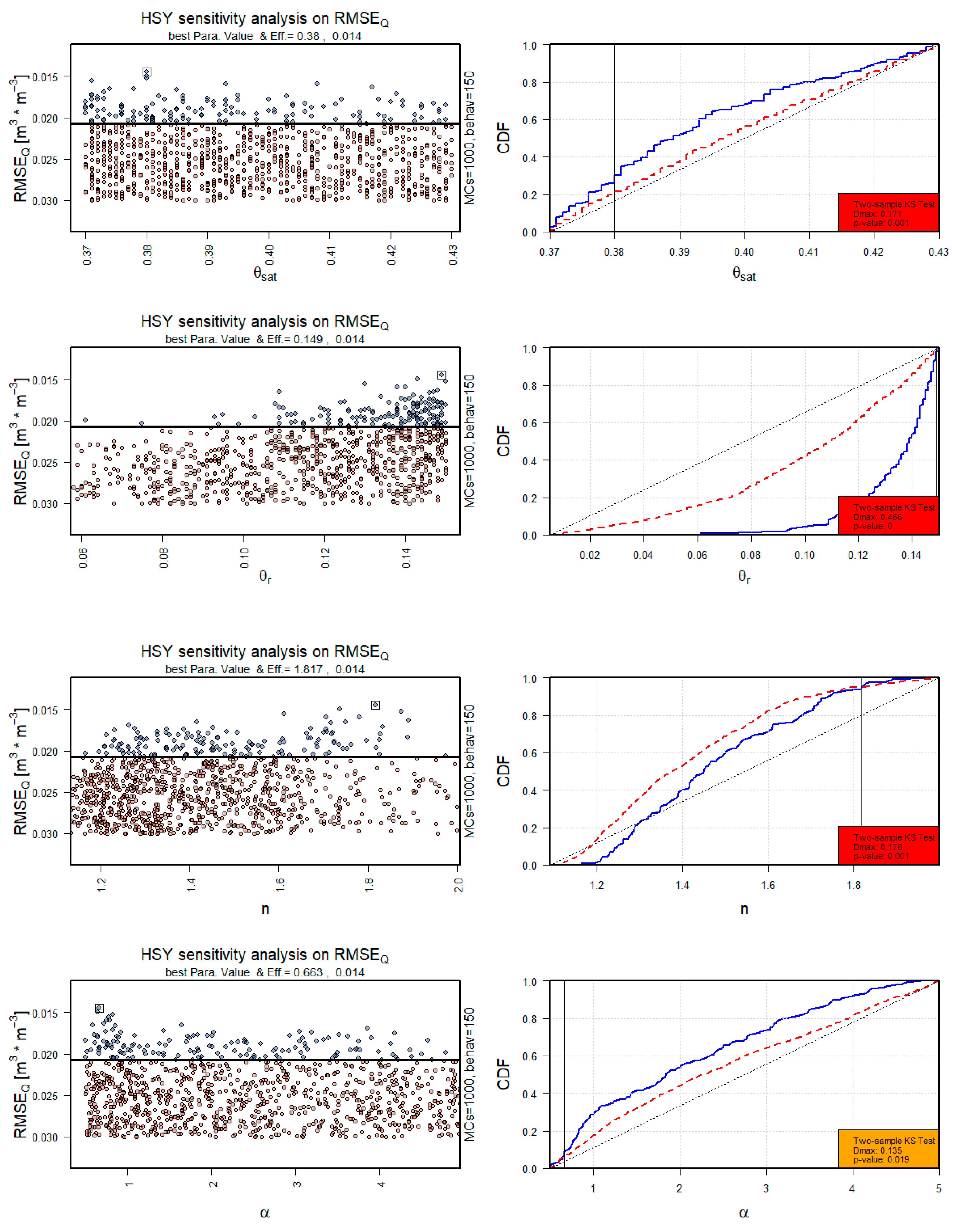
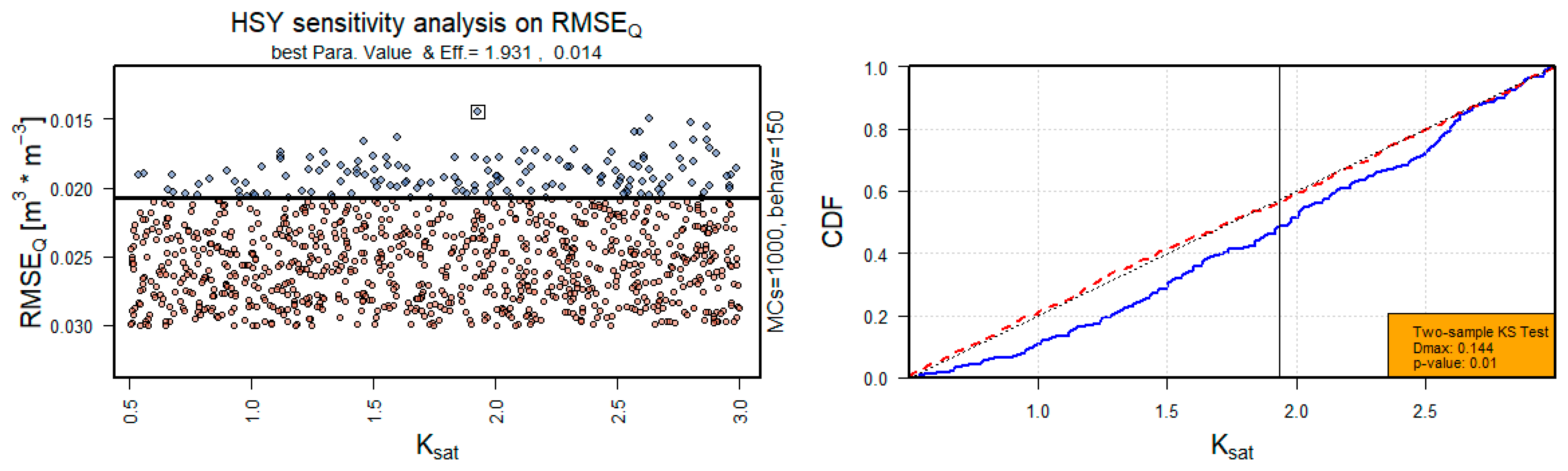
The soil parameters θsat, θr, n, α and Ksat were calibrated for prediction error of simulated volumetric soil water content red to observed data over a period of 2 years (number of observations N = 730). Calibration was done by the Monte-Carlo method [67], where 5000 parameter sets were randomly selected of a range resembling that of values for soils from sand to clay loam, evaluating the prediction on RMSE and RMSEQ to get the minimal divergence of simulated and observed data. Furthermore, a sensitivity analysis was done by the Hornberger-Spear-Young method (HSY) for the 1000 parameter sets with least RMSE and RMSEQ with a behavioral rate of 15% (150 best outcomes) [68]. Sensitivity was tested with a two-sample Kolmogorov-Smirnov Test (KS-Test), defining sensitivity and slight sensitivity as significance p ≤ 0.01 and p ≤ 0.05, respectively, and critical value D0.01 = 0.15 and D0.05 = 0.12, respectively [69].
2.5.3. Validation
Forest growth was simulated with 3PG-Hydro, as well as with 3PG vsn. 2.7, on daily and monthly calculation resolution. We validated each simulation for all stands over the monitored period to see not only how the hydrological sub-model performs but also how the downscaling of temporal resolution affected forest-growth prediction. We simulated soil water content of the ER (depth = 0.6 m) with 3PG-Hydro daily, with the calibrated soil parameters as input. For comparison purposes, we simulated the soil water content of the ER with 3PG vsn. 2.7 on daily resolution. We set the 3PG vsn. 2.7 soil parameters (minimum and maximum available soil water) to the calibrated values of θr and θsat, respectively. We compared the results to measured data at 0.3 m and 0.6 m depth over a 3-year period at Conventwald (N = 1096). To evaluate the effect of temporal downscaling on soil-water processes, we compared percolation prediction by 3PG-Hydro daily to prediction by 3PG-Hydro monthly. Evapotranspiration (ET) simulation was not validated due to non-availability of forest ET data. However, to get an overview of the ET performance, it was simulated with 3PG-Hydro daily and 3PG vsn. 2.7 daily for all stands over the monitored periods and visually evaluated. Furthermore, we simulated ET of a clear-cut (0 trees × hectar−1) area for each stand and visually compared the results to data of actual ET of grass obtained from nearby areas to check how the separated soil evaporation predicted ET without trees. Furthermore, we did a water balance for all stands over the monitored periods.
3. Results
3.1. Calibration
RMSE and RMSEQ, respectively (m3 × m−3), showed almost the same deviation. Apparently, θsat, θr, n and α display a minor difference, while Ksat shows a greater difference. For further evaluation, we decided to use the parameters from the calibration on RMSEQ because our aim was to achieve good performance within water-content range from the first to third quartile. A sensitivity was not visible by examining the outcome of the 5000 parameter sets (Figure A2) but by analysis with HSY (Figure A3). The KS-Test of the parameters obtained with calibration on RMSE led to sensitivity of θsat, θr, α and Ksat and no sensitivity of n. Calibration on RMSEQ led to sensitivity of θsat and θr as well as slight sensitivity of α and Ksat and no sensitivity of n (Figure A3).
3.2. Validation
3.2.1. Forest Growth
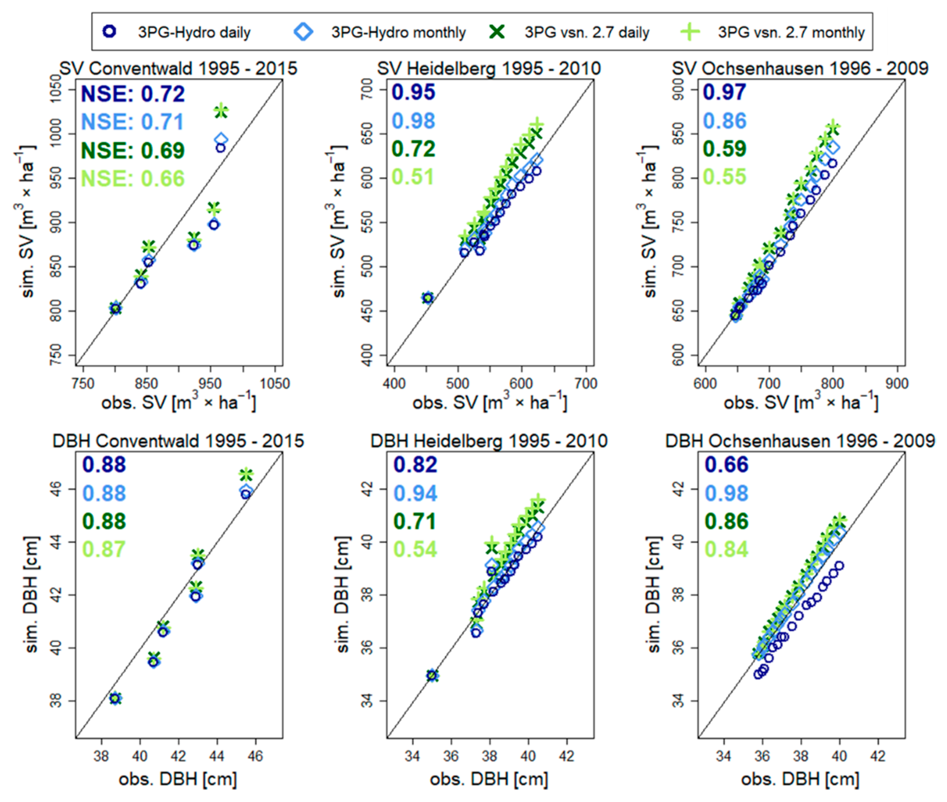
The evaluation of stand-volume (SV) simulation (Figure 2) indicates a better performance of 3PG-Hydro compared to 3PG vsn. 2.7, with almost perfect prediction at Heidelberg and Ochsenhausen. Comparing the prediction of daily versus monthly calculations, the deviation from 3PG-Hydro is of minor significance at Conventwald and Heidelberg, but calculations are better at Ochsenhausen for 3PG vsn. 2.7. The better performance of the daily resolution is evident. For mean diameter at breast height (DBH), a different picture emerges, showing very good and similar performance of all models at Conventwald, better performance of 3PG-Hydro and especially 3PG-Hydro on monthly resolution at Heidelberg and at Ochsenhausen. The worst performance was achieved by 3PG-Hydro daily calculations, while the best and almost perfect prediction what achieved by 3PG-Hydro monthly calculations. However, the RMSE of 3PG-Hydro daily at Ochsenhausen is only 2%, compared to 0.8% of 3PG-Hydro monthly. Generally, DBH simulation by 3PG-Hydro is better on monthly resolution, while 3PG vsn. 2.7 performs better on daily resolution.
3.2.2. Thinning
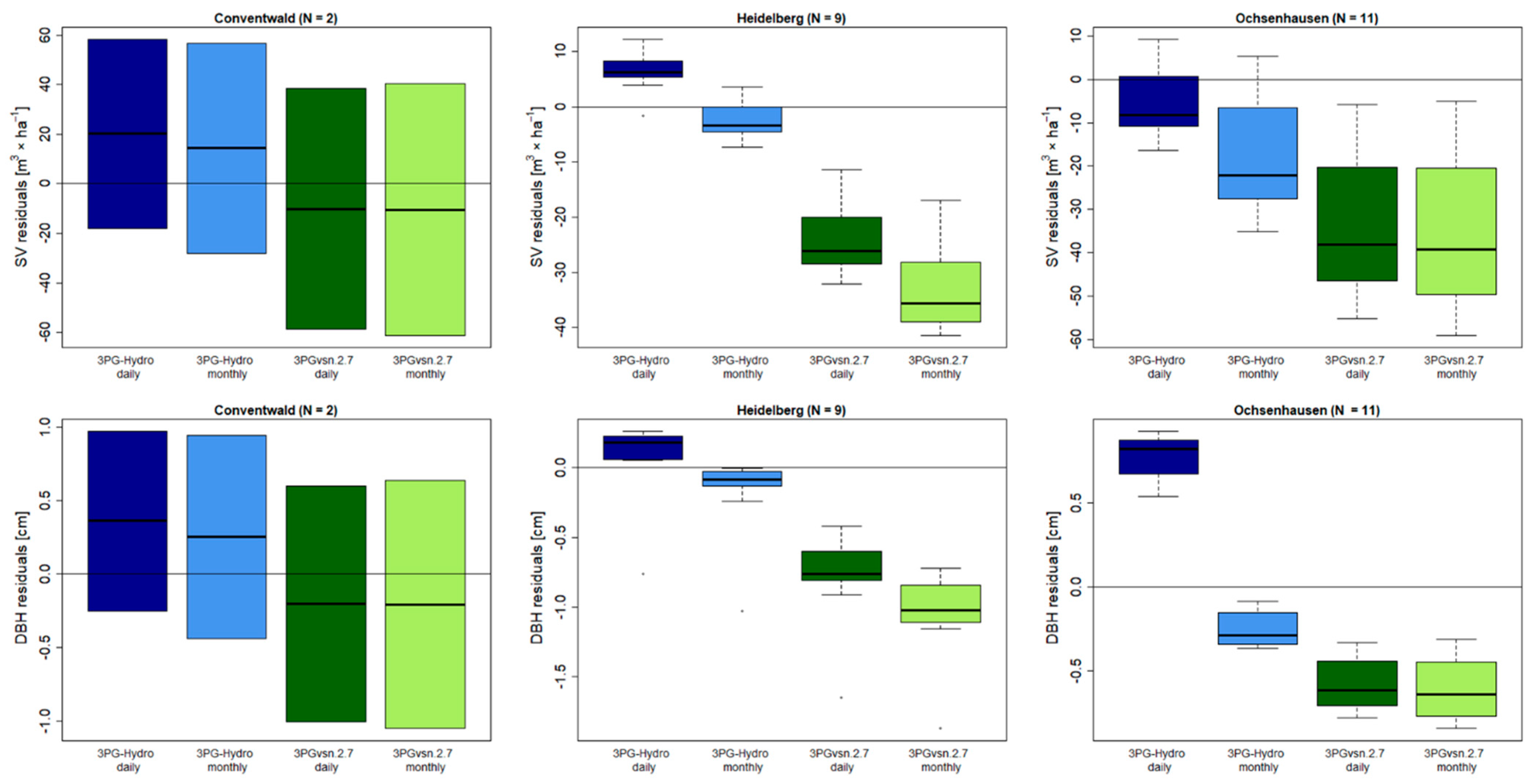
Thinning was applied with very low intensities at Heidelberg, Ochsenhausen and Coventwald (Table A2). Figure 3 displays the residuals (observed data—simulated data) of SV and DBH for the years after a thinning event until the next thinning event. This shows a poorer performance of 3PG-Hydro for low thinning at the Conventwald site (Figure 3). However, the available data for this site are very few (N = 2) and should be interpreted very carefully. For the sites with more data and very low thinning, the performance of 3PG-Hydro was clearly better. 3PG-Hydro underestimates SV and DBH growth after thinning, while 3PG vsn 2.7 overestimates SV and DBH growth after thinning. This is important when it comes to correctly planning thinning to achieve certain yields.
3.2.3. Soil Water Content
Visual reflection of the SW prediction (Figure 4) clearly shows the better predictions of 3PG-Hydro, following the behavior of the observed data and staying within the range of the first (Q1) and third quartile (Q3), with a few exceptions. In contrast, 3PG vsn. 2.7 highly overestimates the observed data and is generally out of range. These observations reflect in the performance evaluation (Table 2), presenting a total RMSE on the mean observed data for 3PG-Hydro of 10% compared to 36% for 3PG vsn 2.7. Within the range of Q1 and Q3, the RMSEQ of 3PG-Hydro is almost six times lower than that of 3PG vsn 2.7. Validated on the mean observed data (NSE), 3PG-Hydro performs worse than the mean of all observed data, but this indicates no failure because the performance within the range is very good (NSEQ = 0.88). In comparison, 3PG vsn. 2.7 not only performs poorly on mean data (NSE) but also within the range (NSEQ), with NSEQ3 clearly indicating the overestimation of high values.
3.3. Evaluation
3.3.1. Percolation
The advantage of daily resolution is better depiction of percolation after high and low precipitation events, whereas monthly resolution takes the mean and thus misses the dynamic variability. This is especially the case for high daily precipitations (Figure A4). At Conventwald, the importance of daily resolution is visible due to the strong reaction to higher rainfall. At Heidelberg and Ochsenhausen, the difference appears minor but is still evident for very significant precipitation events. (Figure A4). The discrepancies at the sites are due to the different soil characteristics and the overall precipitation dynamics.
3.3.2. Evapotranspiration
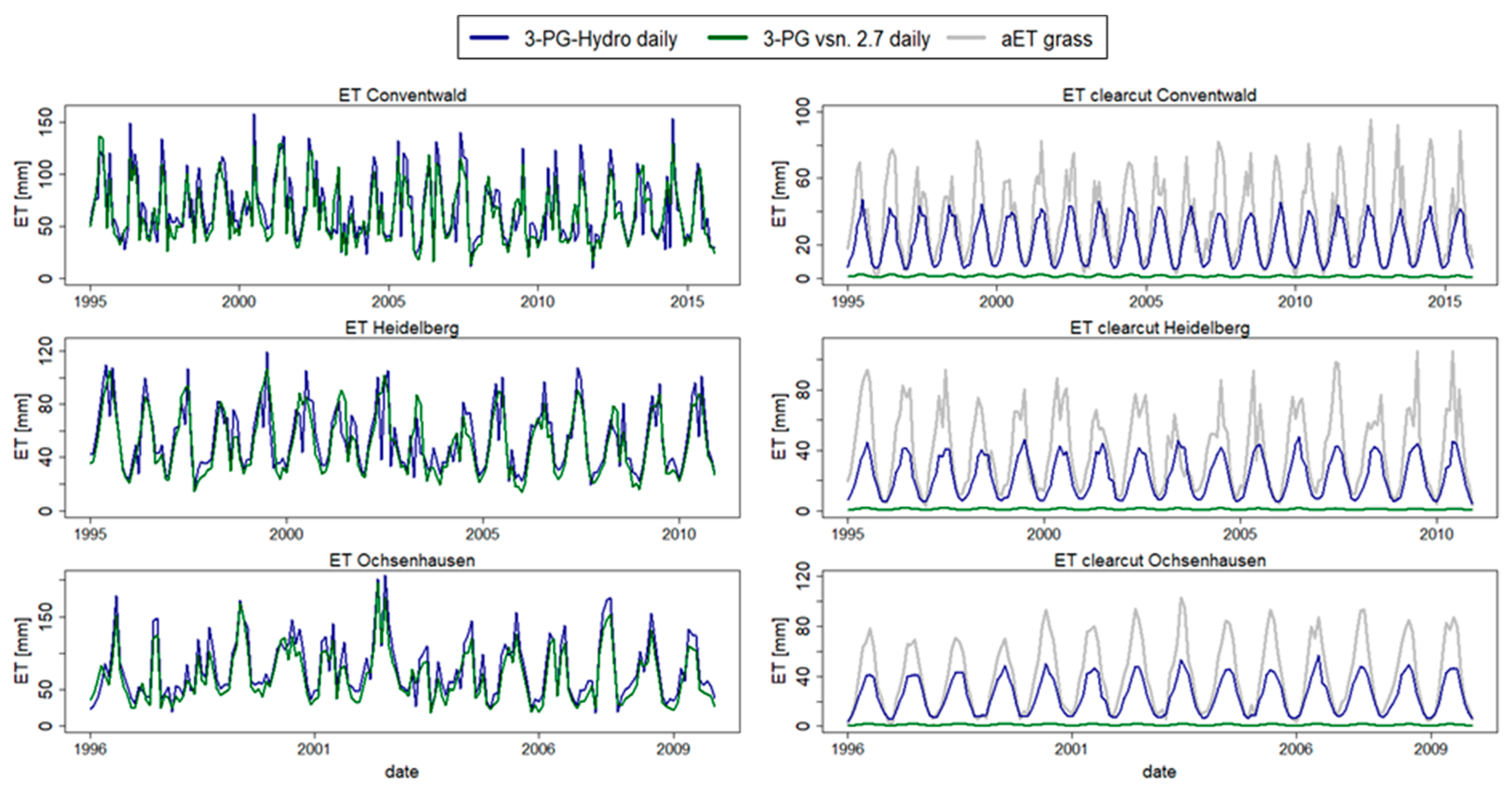
The mean monthly evapotranspiration (ET) simulated on daily resolution by 3PG-Hydro and 3PG vsn 2.7 show very similar behavior between the separated and the original one-mass-flow calculation at all three sites, with only small deviations (Figure A4). In contrast, the clear-cut simulations clearly show the better performance and the advantage of a separation. 3PG-Hydro estimates the evaporation close to the value of actual evaporation of grass in terms of periodicity and quantity, whereas 3PG vsn. 2.7 simulates values close to 0 (Figure A5).
3.3.3. Water Balance
The water balance shows all input, output and storage contents (mm) summed up over the whole observed periods of 20, 16 and 14 years, respectively for each site (Table 3). Input is dominated by rain, with low contribution of snow, depending on, site and not affected by deep capillary rise. Output is clearly dominated by evapotranspiration, with shares of around 90% at Conventwald and Heidelberg, as well as 98.6% at Ochsenhausen, with remaining portion being deep percolation, while runoff plays no role. The end-of-simulation storage depicts water being stored in snow beyond simulation time, as well as a soil water increase of around 25% in the ER (SWER) and DR (SWDR) at Ochsenhausen, whereas changes at the other stands were minor. Comparison to the mean SWER and SWDR of the whole period to check if these changes were only of temporary showed that, indeed, the change of SWER was temporary but that SWDR increase is robust. The comparison also pointed out a SWER decrease of 27% at Heidelberg.
4. Discussion
4.1. The Model
Environmental models combining accurate forest-growth prediction and good SW depiction are scarce but of high importance when it comes to simulation of the effects of future climate change scenarios on forest growth. Our results reflect that the previous version of 3PG did not fulfill the combination of both accurate forest-growth prediction and good SW depiction. However, the updated 3PG-Hydro model achieved a reliable performance, coupling forest growth and soil-water-processes by temporal downscaling, as well as by adding a hydrological sub-model with upgraded modifiers. Daily resolution predicted forest growth better, except for smaller deviations on DBH prediction due to the small magnitude and therefore higher sensitivity of the values. 3PG-Hydro simulated very low thinning better than 3PG vsn. 2.7 because of its daily resolution and more accurate soil water prediction, therefore achieving a higher sensitivity. However, the results are limited due to the low density of data used to analyze the effects of thinning events on forest growth. Higher thinning regimes could not be tested because of the lack of data for validation. However, due to the good separation of evapotranspiration (Figure A5), we assume a better performance of 3PG-Hydro. Further, the particular advantage of a daily simulation is the depiction of variability in precipitation, especially extreme rainfall, and consequently, SW, both being necessary for climate change simulations, where droughts and intense rainfall events are expected to increase [70,71] (Trenberth, 2011; Teuling, 2018). This advantage is reflected in the reaction of percolation to intense rainfall (Figure A4). To further illustrate this point, we created a very extreme scenario. We applied 3PG-Hydro daily to simulate stand volume with precipitation data, where every month had 29 days without rain, followed by one day with 150 mm of rain. We applied 3PG-Hydro monthly with the same precipitation data (interpreted as 150 mm × month−1, daily mean of 5 mm × day−1). We found that the monthly calculation diverges extremely from the daily calculations as a consequence of misrepresenting precipitation details and thus the soil-water processes (Figure 5).
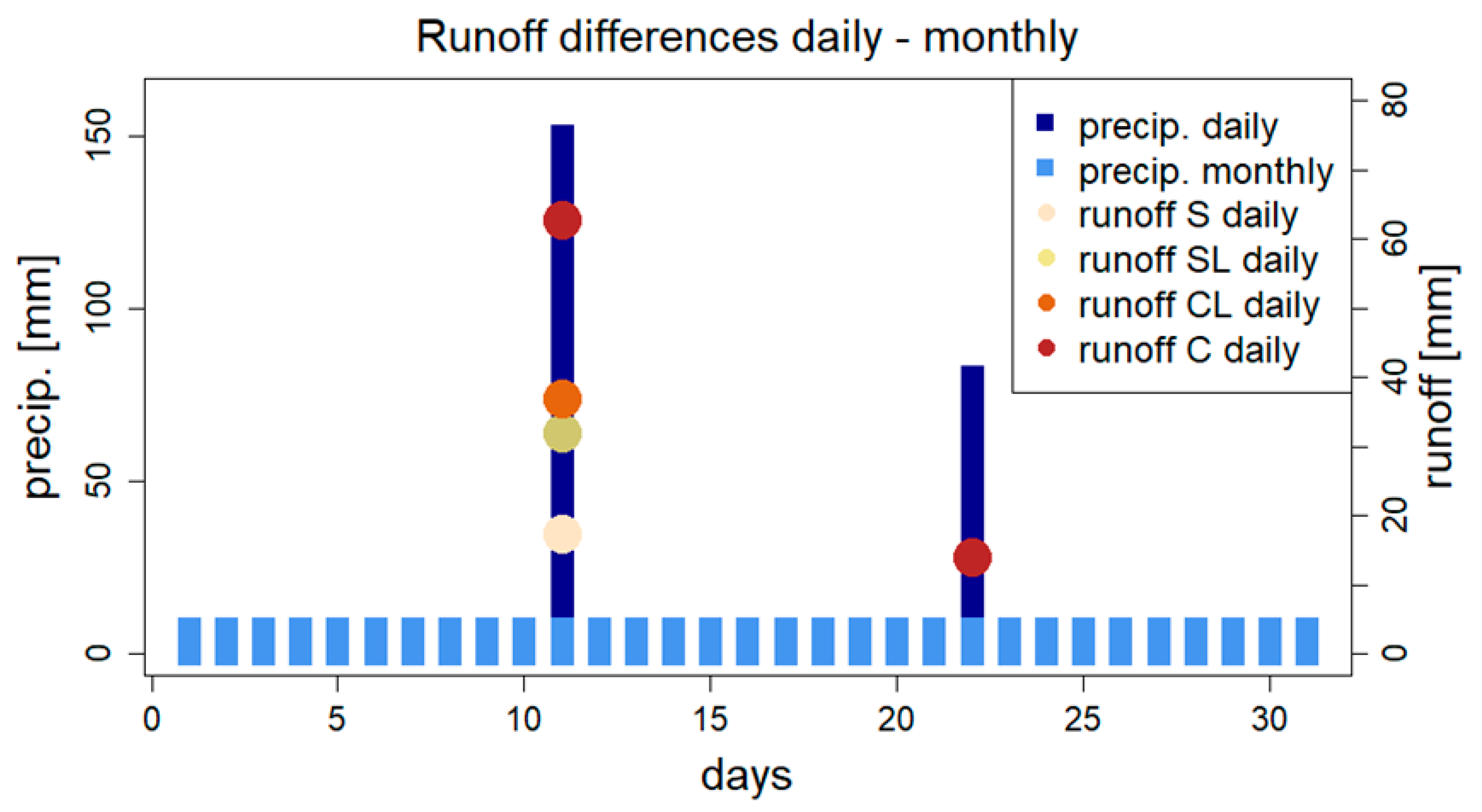
Furthermore, heavy rainfalls lead to runoff formation, which is illustrated in Figure 6, where runoff was predicted by 3PG-Hydro (daily and monthly resolution) with each of the four soil-type presets (Table A1). We used a precipitation scenario of 29 days without rain and 2 days of extreme rainfall (150 mm, 80 mm) as daily input, whereas monthly resolution treated the data as 230 mm × month−1 (daily mean of 7.4 mm × day−1). No runoff was predicted with 3PG-Hydro on monthly resolution due to precipitation being very low. The simulation with daily resolution led to runoff with each soil type in response to the event of 150 mm × day−1. Further, the dependence of runoff magnitude on soil type is evident, indicating the importance of soil texture implementation in the model, which is also reflected in the sensitivity analysis, with four of the five soil parameters being sensitive or slightly sensitive (Section 3.1).
In general, the hydrological sub-model predicted forest growth better than 3PG vsn. 2.7 (Figure 2) and can be verified with a very satisfying outcome, which is also due to its qualified SW prediction at Conventwald (Figure 4). The performance in between the range of observed data (NSEQ = 0.88) is good, especially because, after all, 3PG is a forest-growth model and a complex coupling of many processes, therefore posing difficulty in combining it with other sub-models. Furthermore, the deviations of SW prediction are marginal because only low overestimations of SW were observed, which is extremely important when it comes to modelling water resources in times of drought. On the other hand, 3PG vsn. 2.7 constantly overestimated SW. Certainly, the maximum soil water parameter of 3PG vsn 2.7 can be set lower, improving the overestimation of SW, but this fitted value would diverge from real conditions (θsat). The hydrological processes of runoff, percolation (PC), deep percolation (DP) and capillary rise (CRER, CRDR) can only be vaguely analyzed and interpreted. First, their complexity is very simplified by the sub-model, and second, there is a lack of observed data to compare. Runoff did almost not appear at any site (Table 3), mainly for two reasons: one is the high infiltration (Ksat) and storage capacity of the simulated soils, and the other is that 3PG-Hydro only simulates infiltration based on daily precipitation values, but runoff generation is highly dependent on hourly intensities [16]. This leads to a general underestimation of runoff by 3PG-Hydro. PC, being directly influenced by infiltration and displaying the variability of precipitation and soil texture, appeared in high rates at Conventwald (Table 3). Therefore, the accuracy of SWER simulation can be assessed as good. At Heidelberg, PC also played a major role (Table 3) due to the specific soil characteristics of relatively high hydraulic conductivities (sandy loam, Table A1). At Ochsenhausen, it only played a minor role (Table 3) due to the high storage capacity and low hydraulic conductivity of the set soil (clay loam, Table A1). The outflow to the water table is classified as deep percolation (DP) and not groundwater recharge due to it being only one-dimensional (vertical) and therefore not representing important lateral-flow processes, resulting in no accurate recharge. However, DP values can be used to assess forest management (e.g., thinning, rejuvenation, species) influences on water yield. DP showed a similar pattern as PC due to the specific soil characteristics and was of higher importance at Conventwald and Heidelberg but played no role at Ochsenhausen (Table 3). Capillary rise only becomes important in soils under very dry conditions, which was not the case at the test sites (Table 3).
The separation of ET was successfully carried out because of only small differences between the ET simulations of 3PG-Hydro and 3PG vsn. 2.7 (Figure A5). This implies that separation did not lead to over- or underestimation of ET. The great advantage of a separated ET calculation is the improvement in prediction of forest management effects (e.g., clear-cut, Figure A5) on forest and water processes. The generally high shares of ET on output (Table 3) are a peculiarity of 3PG due to ET being calculated on potential VPD, with all intercepted rain gets fully evaporated [9]. For further improvement of 3PG-Hydro, a surface model could be integrated to simulate lateral soil water flow, runoff could be enhanced by adding hourly precipitation intensities for heavy rainfall events and evapotranspiration calculation could be further improved. However, it is important to consider the trade-off between model precision and relevance and carefully add complexity to the relatively easy-to-handle 3PG and 3PG-Hydro models.
4.2. Advantages for Forest Management Application
The motivation for develop ing 3PG-Hydro was to enhance the simulation of forest management measures on both growth and water cycle, especially in the view of a changing climate and drought. 3PG-Hydro can effectively help to investigate how forest management measures (e.g., thinning) (1) can improve individual tree growth by limiting decrease in SW in times of drought and (2) increase the water yield (deep percolation and runoff) for ecological, as well as economical (commercial water), reasons. This is achieved by (1) individualization of each site’s soil characteristics with a preset or by specific parametrization, (2) simulating percolation and runoff processes, (3) separating transpiration and evapotranspiration to predict good evapotranspiration, even if high thinning is applied, (4) calculating in daily time steps to simulate variation and especially drought better and (5) improving the soil-water modifier. This results in a growth simulation more sensitive to forest management measures and variability in soil water. This is a crucial base for evaluating forest water service and studies of its cost-effectiveness [72].
5. Conclusions
3PG-Hydro achieved its set purpose of coupling higher temporal resolved forest-growth prediction with a reliable soil-water model. In its entity, 3PG-Hydro performed very well for all validated and evaluated upgrades compared to 3PG vsn. 2.7. Moreover, the novel development (daily temporal resolution, detailed soil-water processes) aligns with the specific research questions and the crucial need to analyze forest-growth interactions with water and soil processes. 3PG-Hydro can, in general, better simulate forest growth (stand volume, average diameter), as well as details of soil and water processes after thinning events. However, the marginal benefit is not very high regarding intensive data needs and increased model complexity. Overall, 3PG-Hydro offers a good balance of input (low data intensity) and output (relevant decision parameters) crucial in analysis of forest water interactions under changing climate conditions. This is essential to the study of forest drought and analysis of thinning effects on forest growth, water and carbon values.
Author Contributions
Conceptualization, R.Y.; methodology, software, validation, formal analysis and investigation, R.Y. and M.D.; resources and data curation, R.Y.; writing—original draft preparation, review and editing, visualization, R.Y. and M.D.; supervision, project administration, funding acquisition, R.Y. All authors have read and agreed to the published version of the manuscript.
Funding
This research received no external funding.
Institutional Review Board Statement
Not applicable.
Informed Consent Statement
Not applicable.
Acknowledgments
We acknowledge Forest research Institute of Baden Württemberg (FVA-BW) and ICP-Forests for providing the forest data and Gesa Meyer for guidance at the early stage of this research. The study is supported by the activities and exchanges in project “PESFOR-W” and “DecisionES” funded by the European Commission.
Conflicts of Interest
The authors declare no conflict of interest.
Appendix A
Appendix A.1. Additional Equations
Appendix A.1.1. Daily Melting Snow Snowmelt (mm × day−1)
Appendix A.1.2. Infiltration I and Runoff Runoff Respectively (mm × day−1)
Appendix A.1.3. DR Soil Water Saturation SWDRsat (mm)
Appendix A.1.4. Field Capacity (FC) and Wilting Point (WP)
Calculation of water content Θ (m3 × m−3) at FC (−1500 kPa = 3.365 m) and WP (−33 kPa = 152.961 m) after VGM:
where h is hydraulic head (m), α is Van-Genuchten α (m−1) and n is Van-Genuchten n (−), using it as input for calculation of volumetric FC (m3 × m−3) and WP (m3 × m−3):
where θsat is the volumetric saturation water content and θr is the volumetric residual water content (m3 × m−3).
Appendix A.1.5. Change by Depth
Change of field capacity in DR θfcDR (m3 × m−3):
where θfc is the volumetric field capacity (m3 × m−3) and fθDR is the compaction factor of 20% (−).
Change of hydraulic conductivity in DR KsatDR (m × day−1):
where Ksat is saturated hydraulic conductivity (m × day−1) and fkDR is the compaction factor (for sand: 1, sandy loam: 0.8, clay loam: 0.6 and clay: 0.5).
Appendix A.1.6. Deep Percolation, DP, and Deep Capillary Rise, CRDR, Respectively (mm × day−1)
Appendix A.1.7. Water Content of the ER ΘER and DR ΘDR, Respectively (m3 × m−3)
Appendix A.1.8. Hydraulic Head of DR as a Function of DR Water Content hDR(ΘDR) (m)
Appendix A.1.9. Unsaturated hydraulic conductivity of ER and DR as a function of ER and DR water content, Ku(ΘER) and KuDR(ΘDR), respectively (m × day−1)
Appendix A.1.10. Residual mean square error RMSE
Appendix A.2. Preset Soil Parameters

Table A1.
VGM preset soil parameters. Values from Jabro (1992), Gootman et al. (2020), Hodnett & Tomasella, (2002) and Nemes et al. (2001) were considered and further modified.
Table A1.
VGM preset soil parameters. Values from Jabro (1992), Gootman et al. (2020), Hodnett & Tomasella, (2002) and Nemes et al. (2001) were considered and further modified.
| Soil Type | θsat (m3 × m−3) | θres (m3 × m−3) | n (−) | α (m−1) | Ksat (m × day−1) |
|---|---|---|---|---|---|
| sand | 0.38 | 0.02 | 1.55 | 4 | 3.50 |
| sandy loam | 0.4 | 0.08 | 1.35 | 3.5 | 1 |
| clay loam | 0.44 | 0.1 | 1.25 | 2.8 | 0.4 |
| clay | 0.5 | 0.12 | 1.1 | 2.4 | 0.1 |
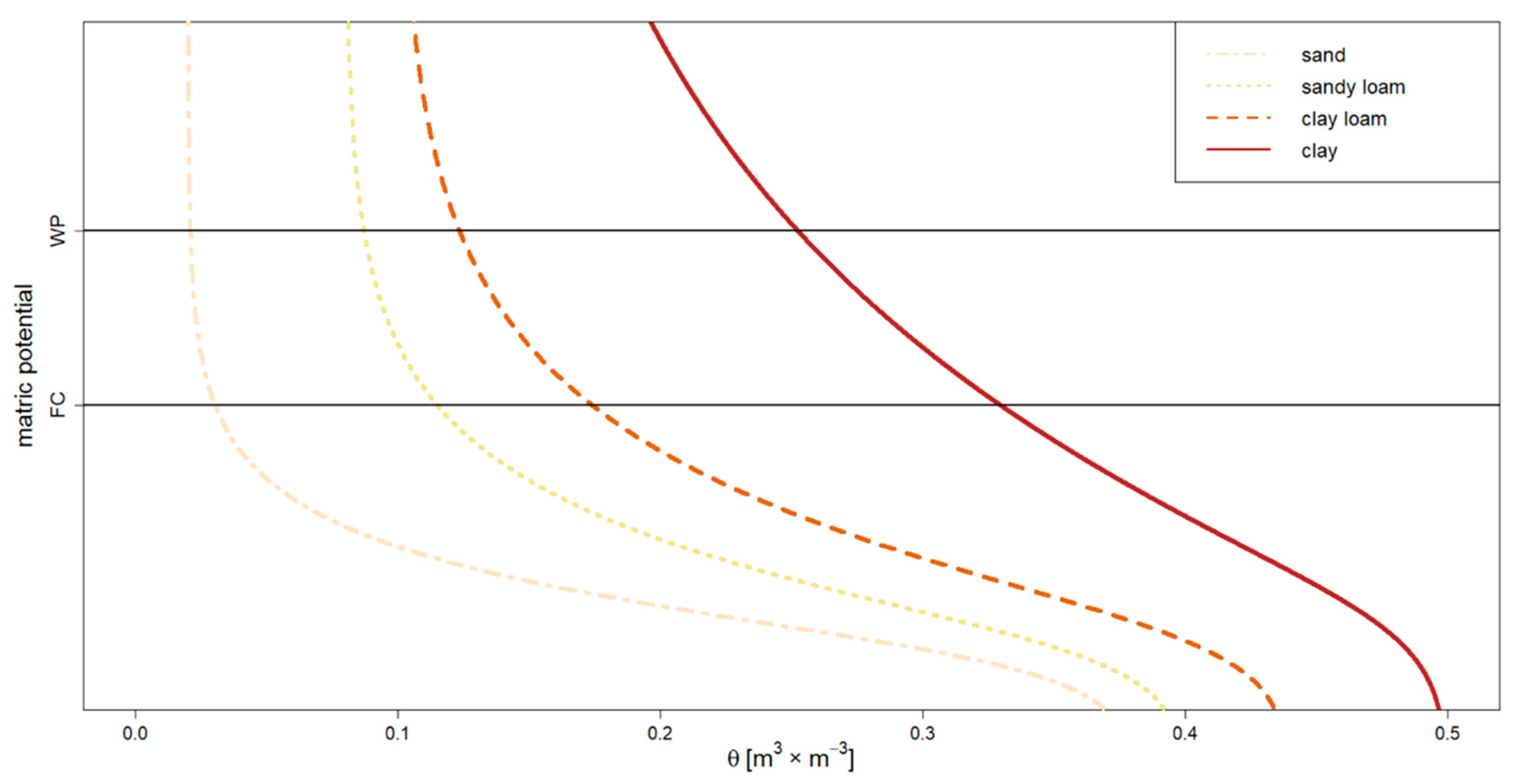
Figure A1.
The figure displays the water retention curves of each pre-set soil of 3PG-Hydro.

Appendix A.3. Thinning Regimes
Table A2.
Three thinning regimes applied at the sites. Stems are the stems before thinning took place. The percentage is the proportion of thinned stems to stems before thinning.
Table A2.
Three thinning regimes applied at the sites. Stems are the stems before thinning took place. The percentage is the proportion of thinned stems to stems before thinning.
| Age | Stems | Thinned Stems | Method | |
|---|---|---|---|---|
| Conventwald | 80 | 528 | 60 (11.4%) | Below |
| 85 | 468 | 52 (11.1%) | Below | |
| Heidelberg | 89 | 380 | 20 (5.3%) | Below |
| 91 | 360 | 15 (4.2%) | Below | |
| Ochsenhausen | 77 | 496 | 4 (0.8%) | Middle |
| 79 | 492 | 8 (1.6%) | Middle | |
| 80 | 484 | 4 (0.8%) | Middle |
Appendix A.4. Additional Calibration Results
Figure A2.
The 5000 MC calibration runs for θr (m3 × m−3), n (−), α (m−1), Ksat (m × day−1) on the RMSE and RMSEQ delivered the following results, with red dots marking the lowest RMSE or RMSEQ.
Figure A2.
The 5000 MC calibration runs for θr (m3 × m−3), n (−), α (m−1), Ksat (m × day−1) on the RMSE and RMSEQ delivered the following results, with red dots marking the lowest RMSE or RMSEQ.

Figure A3.
The following figures present the outcomes of the sensitivity analysis by HSY method and with a two-sample KS-Test on RMSE and RMSEQ with θsat and θr (m3 × m−3), n (−), α (m−1) and Ksat (m × day−1). The colour of the legend of CDF-plot (right) indicates if it is sensitive (red) or slighlty sensitive (orange). Even though the parameter n is marked as sensitive, it was rejected as not sensitive because of the similarity between behavioral and non-behavioral.


Appendix A.5. Additional Figures
Figure A4.
Variation of percolation from ER to DR (PC) due to daily or monthly calculation resolution, where ∆ perc. (mm × day−1) is the difference between the simulated percolation with daily and monthly resolution. Monthly precipitation (precip. monthly, mm × day−1) is the daily mean of monthly precipitation.

Figure A5.
Evapotranspiration (mm × month−1) simulations by 3-PG-Hydro and 3-PG vsn. 2.7 calculated with daily resolution and displayed as monthly sum. The three plots on the left show the ET simulation at all three stands. The plots on the right display the clear-cut simulation (0 trees × hectar−1) for each stand. It is compared to observed actual evaporation of grassland at the site.

References
- Chazdon, R.L. Beyond deforestation: Restoring forests and ecosystem services on degraded lands. Science 2008, 320, 1458–1460. [Google Scholar] [CrossRef] [PubMed] [Green Version]
- Bredemeier, M.; Cohen, S.; Godbold, D.L.; Lode, E.; Pichler, V.; Schleppi, P. Forest Management and the Water Cycle. An Ecosystem-Based Approach; Springer: Berlin/Heidelberg, Germany, 2011. [Google Scholar]
- Yousefpour, R.; Temperli, C.; Jacobsen, J.B.; Thorsen, B.J.; Meilby, H.; Lexer, M.J.; Lindner, M.; Bugmann, H.; Borges, J.G.; Palma, J.H.N.; et al. A framework for modeling adaptive forest management and decision making under climate change. Ecol. Soc. 2017, 22, 40. [Google Scholar] [CrossRef]
- Campos Arce, J.J. Forests, Inclusive and Sustainable Economic Growth and Employment. Background Study Prepared for the 14th Session of the United Nations Forum on Forests; United Nations Forum on Forests: New York, NY, USA, 2019. [Google Scholar]
- Levia, D.F.; Carlyle-Moses, D.E.; Ilida, S.; Michalzik, B.; Nanko, K.; Tischer, A. Forest-Water Interactions. Ecological Studies; Springer: Berlin/Heidelberg, Germany, 2020. [Google Scholar]
- Hewlett, J.D. Principles of Forest Hydrology; University of Georgia Press: Athens, GA, USA, 1969. [Google Scholar]
- Sturtevant, B.R.; Fall, A.; Kneeshaw, D.D.; Simon, N.P.P.; Papaik, M.J.; Berninger, K.; Doyon, F.; Morgan, D.G.; Messier, C. A toolkit modeling approach for sustainable forest management planning: Achieving balance between science and local needs. Ecol. Soc. 2007, 12, 7. [Google Scholar] [CrossRef] [Green Version]
- Landsberg, J.J.; Waring, R.H. A generalised model of forest productivity using simplified concepts of radiation-use efficiency, carbon balance and partitioning. For. Ecol. Manag. 1997, 95, 209–228. [Google Scholar] [CrossRef]
- Landsberg, J.J.; Sands, P.J. Physiological Ecology of Forest Production. Principles, Processes and Models; Terrestrial Ecology; Academic Press: London, UK, 2010. [Google Scholar]
- Landsberg, J.J.; Waring, R.H.; Coops, N.C. Performance of the forest productivity model 3-PG applied to a wide range of forest types. For. Ecol. Manag. 2003, 172, 199–214. [Google Scholar] [CrossRef]
- Sands, P.J. 3PGpjs vsn 2.4—A User-Friendly Interface to 3PG, the LANDSBERG and Waring Model of Forest Productivity. Technical Report. No. 140; CRC Sustainable Production Forestry: Hobart, Australia, 2004. [Google Scholar]
- Sands, P.J. 3PGpjs User Manual. Software Versions: 3PGpjs vsn 2.7/3PG vsn September 2010. 2010. Available online: chrome-extension://bocbaocobfecmglnmeaeppambideimao/pdf/viewer.html?file=https%3A%2F%2F3pg.forestry.ubc.ca%2Ffiles%2F2014%2F04%2F3PGpjs_UserManual.pdf (accessed on 15 November 2021).
- Meyer, G.; Black, T.A.; Jassal, R.S.; Nesic, Z.; Coops, N.C.; Christen, A.; Fredeen, A.L.; Spittlehouse, D.L.; Grant, N.J.; Foord, V.N.; et al. Simulation of net ecosystem productivity of a lodgepole pine forest after mountain pine beetle attack using a modified version of 3-PG. For. Ecol. Manag. 2018, 412, 41–52. [Google Scholar] [CrossRef]
- Blöschl, G.; Sivapalan, M. Scale issue in hydrological modelling: A review. Hydrol. Process. 1995, 9, 251–290. [Google Scholar] [CrossRef]
- Skøien, J.O.; Bloschl, G.; Western, A.W. Characteristic space scales and timescales in hydrology. Water Resour. Res. 2003, 39, 1304. [Google Scholar] [CrossRef]
- Dunne, T.; Zhang, W.; Aubry, B.F. Effects of rainfall, vegetation and microtopography on infiltration and runoff. Water Resour. Res. 1991, 27, 2271–2285. [Google Scholar] [CrossRef]
- Chang, M. Forest Hydrology: An Introduction to Water and Forests, 2nd ed.; Taylor & Francis: Abingdon, UK, 2006. [Google Scholar]
- Renger, M.; Strebel, O. Jährliche Grundwasserneubildung in Abhängigkeit von Bodennutzung und Bodeneigenschaften. Wasser Boden 1980, 32, 362–366. [Google Scholar]
- Kučera, A.; Same, P.; Bajer, A.; Skene, K.; Vichta, T.; Vranová, V.; Meena, R.S.; Datta, R. Forest soil water in landscape context. In Soil Moisture Importance; Meena, R.S., Datta, R., Eds.; InTech: London, UK, 2020. [Google Scholar]
- Scheffer, F.; Schachtschabel, P.; Blume, H.P.; Brümmer, G.W.; Horn, R.; Kandeler, E.; Kögel-Knabner, I.; Kretzschmar, R.; Stahr, K.; Wilke, B.-M. Lehrbuch der Bodenkunde; 16. Auflage; Springer: Berlin/Heidelberg, Germany, 2010. [Google Scholar]
- Saxton, K.E.; Rawls, W.J. Soil Water Characteristic Estimates by Texture and Organic Matter for Hydrologic Solutions. Soil Sci. Soc. Am. J. 2006, 70, 1569–1578. [Google Scholar] [CrossRef] [Green Version]
- Adams, R.S.; Black, T.A.; Fleming, R.L. Evapotranspiration and surface conductance in a high elevation, grass-covered forest clearcut. Agric. For. Meteorol. 1991, 56, 173–193. [Google Scholar] [CrossRef] [Green Version]
- Marc, V.; Robinson, M. The long-term water balance (1972–2004) of upland forestry and grassland at Plynlimon, mid-Wales. Hydrol. Earth Syst. Sci. 2007, 11, 44–60. [Google Scholar] [CrossRef] [Green Version]
- Baldocchi, D.; Ryu, Y. A Synthesis of Forest Evaporation Fluxes—From Days to Years—As Measured with Eddy Covariance. In Forest Hydrology and Biogeochemistry; Springer: Dordrecht, The Netherlands, 2011; pp. 101–116. [Google Scholar]
- Lode, E.; Leivits, M. The LiDAR-based topo-hydrological modelling of the Nigula mire, SW Estonia. Est. J. Earth Sci. 2011, 60, 232–248. [Google Scholar] [CrossRef]
- Vereecken, H.; Weynants, M.; Javaux, M.; Pachepsky, Y.; Schaap, M.G.; van Genuchten, M. Using Pedotransfer Functions to Estimate the van Genuchten-Mualem Soil Hydraulic Properties: A Review. Vadose Zone J. 2010, 9, 795–820. [Google Scholar] [CrossRef]
- van Genuchten, M.T. A Closed-form equation for predicting the hydraulic conductivity of unsaturated soils. Soil Sci. Soc. Am. J. 1980, 44, 892–898. [Google Scholar] [CrossRef] [Green Version]
- Mualem, Y. A new model for predicting the hydraulic conductivity of unsaturated porous media. Water Resour. Res. 1976, 12, 513–522. [Google Scholar] [CrossRef] [Green Version]
- Tickle, P.K.; Coop, N.C.; Hafner, S.D.; The Bago Science Team. Assesing forest productivity at local scales across a native eucalypt forest using a process model, 3PG-SPATIAL. For. Ecol. Manag. 2001, 152, 275–291. [Google Scholar] [CrossRef]
- Augustynczik, A.L.D.; Yousefpour, R. Assessing the synergistic value of ecosystem services in European beech forests. Ecosyst. Serv. 2021, 49, 101264. [Google Scholar] [CrossRef]
- Feikema, P.M.; Morris, J.D.; Beverly, C.R.; Collopy, J.J.; Baker, T.G.; Lane, P.N. Validation of plantation transpiration in south-eastern Australia estimated using the 3PG+ forest growth model. For. Ecol. Manag. 2010, 260, 663–678. [Google Scholar] [CrossRef]
- Almeida, A.C.; Sands, P.J. Improving the ability of 3PG to model the water balance of forest plantations in contrasting environments. Ecohydrology 2015, 9, 610–630. [Google Scholar] [CrossRef]
- Groenendyk, D.G.; Ferre, P.; Thorp, K.R.; Rice, A.K. Hydrologic-process-based soil texture classifications for improved visualization of landscape function. PLoS ONE 2015, 10, e0131299. [Google Scholar]
- Brinkmann, N.; Eugster, W.; Buchmann, N.; Kahmen, A. Species-specific differences in water uptake depth of mature temperate trees vary with water availability in the soil. Plant Biol. 2018, 21, 71–81. [Google Scholar] [CrossRef] [PubMed] [Green Version]
- Hock, R. Temperature index melt modelling in mountain areas. J. Hydrol. 2003, 282, 104–115. [Google Scholar] [CrossRef]
- Rango, A.; Martinec, J. Revisiting the degree-day method for snowmelt computations. JAWRA J. Am. Water Resour. Assoc. 1995, 31, 657–669. [Google Scholar] [CrossRef]
- Ismail, M.F.; Bogacki, W.; Muhammad, N. Degree day factor models for forecasting the snowmelt runoff for Naran watershed. Sci. Int. 2015, 27, 1951–1959. [Google Scholar]
- Fassnacht, S.R.; López-Moreno, J.I.; Ma, C.; Weber, A.N.; Pfohl, A.K.D.; Kampf, S.K.; Kappas, M. Spatio-temporal snowmelt variability across the headwaters of the Southern Rocky Mountains. Front. Earth Sci. 2017, 11, 505–514. [Google Scholar] [CrossRef]
- Yang, Y.; Donohue, R.J.; McVicar, T. Global estimation of effective plant rooting depth: Implications for hydrological modeling. Water Resour. Res. 2016, 52, 8260–8276. [Google Scholar] [CrossRef] [Green Version]
- Raissi, F.; Müller, U.; Meesenburg, H. Ermittlung der effektiven Durchwurzelungstiefe von Forststandorten. LBEG. Geofakten 2009, 9, 1–7. [Google Scholar]
- Lehnhardt, F.; Brechtel, H.M. Durchwurzelungs- und Schöpftiefen von Waldbeständen verschiedener Baumarten und Altersklassen bei unterschiedlichen Standortverhältnissen. Allgem. Forst-u. Jagdzeitg. 1980, 151, 120–127. [Google Scholar]
- Jabro, J.D. Estimation of saturated hydraulic conductivity of soils from particle size distribution and bulk density data. Trans. ASAE 1992, 35, 557–560. [Google Scholar] [CrossRef]
- Gootman, K.S.; Kellner, E.; Hubbart, J.A. A comparison and validation of saturated hydraulic conductivity models. Water 2020, 12, 2040. [Google Scholar] [CrossRef]
- Hodnett, M.; Tomasella, J. Marked differences between van Genuchten soil water-retention parameters for temperate and tropical soils: A new water-retention pedo-transfer functions developed for tropical soils. Geoderma 2002, 108, 155–180. [Google Scholar] [CrossRef]
- Nemes, A.; Lilly, A.; Wösten, H. Development of soil hydraulic pedotransfer functions on a European scale: Their usefulness in the assessment of soil quality. In Sustaining the Global Farm; Stott, D.E., Mohtar, R.H., Steinhardt, G.C., Eds.; International Soil Conservation Organization: Aberdeen, UK, 2001. [Google Scholar]
- Nimmo, J.R. Porosity and pore size distribution. Encycl. Soils Environ. 2004, 3, 295–303. [Google Scholar]
- Reynolds, W.D.; Drury, C.F.; Tan, C.S.; Fox, C.A.; Yang, X.M. Use of indicators and pore volume-function characteristics to quantify soil physical quality. Geoderma 2009, 152, 252–263. [Google Scholar] [CrossRef]
- Craul, P.J. Soil compaction on heavily used sites. J. Arboric. 1994, 20, 109–117. [Google Scholar]
- Tomasella, J.; Hodnett, M.G. Soil Hydraulic Properties and Van Genuchten Parameters for an Oxisol under Pasture in Central Amazonia. In Amazonian Deforestation and Climate; Gash, J.H.C., Nobre, C.A., Robert, J.M., Victoria, R.L., Eds.; J. Wiley and Sons: New York, NY, USA, 1996; pp. 101–124. [Google Scholar]
- Lebon, E.; Dumas, V.; Pieri, P.; Schultz, H.R. Modelling the seasonal dynamics of the soil water balance of vineyards. Funct. Plant Biol. 2003, 30, 699–710. [Google Scholar] [CrossRef]
- Nyberg, L. Water flow path interactions with soil hydraulic properties in till soil at Gårdsjön, Sweden. J. Hydrol. 1995, 170, 255–275. [Google Scholar] [CrossRef]
- Ren, X.; Santamarina, J. The hydraulic conductivity of sediments: A pore size perspective. Eng. Geol. 2018, 233, 48–54. [Google Scholar] [CrossRef] [Green Version]
- Flint, A. Use of pristley-taylor evaporation equation for Soil water limited conditions in a small forest clearcut. Agric. For. Meteorol. 1991, 56, 247–260. [Google Scholar] [CrossRef]
- Eckmüller, O. Allometric relations to estimate needle and branch mass of Norway spruce and Scots pine in Austria. Austrian J. For. Sci. 2006, 123, 7–15. [Google Scholar]
- Kang, Y.X.; Lu, G.H.; Wu, Z.Y.; He, H. Comparison and analysis of bare soil evaporation models combined with ASTER data in Heihe River Basin. Water Sci. Eng. 2009, 2, 16–27. [Google Scholar]
- Mahfouf, J.F.; Noilhan, J. Comparative study of various formulations of evaporations from bare soil using in situ data. J. Appl. Meteorol. 1991, 30, 1354–1365. [Google Scholar] [CrossRef] [Green Version]
- Daamen, C.C.; Simmonds, L.P. Measurement of evaporation from bare soil and its estimation using surface resistance. Water Resour. Res. 1996, 32, 1393–1402. [Google Scholar] [CrossRef]
- Lindroth, A. Aerodynamic and canopy resistance of short-rotation forest in relation to leaf area index and climate. Boundary-Layer Meteorol. 1993, 66, 265–279. [Google Scholar] [CrossRef]
- Bond-Lamberty, B.; Gower, S.T.; Amiro, B.; Ewers, B.E. Measurement and modelling of bryophyte evaporation in a boreal forest chronosequence. Ecohydrology 2011, 4, 26–35. [Google Scholar] [CrossRef]
- Han, J.; Zhou, Z. Dynamics of soil water evaporation during soil drying: Laboratory experiment and numerical analysis. Sci. World J. 2013, 2013, 240280. [Google Scholar] [CrossRef] [PubMed] [Green Version]
- Nobel, P.S.; Cui, M. Hydraulic conductances of the soil, the root-soil air gap, and the root: Changes for desert succulents in drying soil. J. Exp. Bot. 1992, 43, 319–326. [Google Scholar] [CrossRef] [Green Version]
- Ritchie, J.T. Model for predicting evaporation from a row crop with incomplete cover. Water Resour. Res. 1972, 8, 1204–1213. [Google Scholar] [CrossRef] [Green Version]
- Trotsiuk, V.; Hartig, F.; Cailleret, M.; Babst, F.; Forrester, D.I.; Baltensweiler, A.; Buchmann, N.; Bugmann, H.; Gessler, A.; Gharun, M.; et al. Assessing the response of forest productivity to climate extremes in Switzerland using model–data fusion. Glob. Chang. Biol. 2020, 26, 2463–2476. [Google Scholar] [CrossRef] [PubMed]
- Schober, R. Ertragstafel wichtiger Baumarten; J.D. Sauerländer’s Verlag: Frankfurt, Germany, 1975. [Google Scholar]
- Wirth, C.; Schumaker, J.; Detlef, S.E. Generic biomass functions for Norway Spruce in Central Europe—A meta-analysis approach towards prediction and uncertainty estimation. Tree Physiol. 2004, 24, 121–139. [Google Scholar] [CrossRef] [PubMed] [Green Version]
- Nash, J.E.; Sutcliffe, J.V. River flow forecasting through conceptual models part I—A discussion of principles. J. Hydrol. 1970, 10, 282–290. [Google Scholar] [CrossRef]
- Metropolis, N.; Ulam, S. The Monte Carlo method. J. Am. Stat. Assoc. 1949, 44, 335–341. [Google Scholar] [CrossRef]
- Spear, R.C.; Hornberger, G.M. Eutrophication in peel-inlet—II. identification of critical uncertainties via generalized sensitivity analysis. Water Res. 1978, 14, 43–49. [Google Scholar] [CrossRef]
- Wilcox, R. Chapter 5—Comparing two groups. Statistical modeling and decision science. In Introduction to Robust Estimation and Hypothesis Testing, 4th ed.; Academic Press: Cambridge, MA, USA, 2017. [Google Scholar]
- Trenberth, K.E. Changes in precipitation with climate change. Clim. Res. 2011, 47, 123–138. [Google Scholar] [CrossRef] [Green Version]
- Teuling, A.J. A hot future for European droughts. Nat. Clim. Chang. 2018, 8, 364–365. [Google Scholar] [CrossRef]
- Valatin, G.; Ovando, P.; Abildtrup, J.; Accastello, C.; Andreucci, M.; Chikalanov, A.; El Mokaddem, A.; Garcia, S.; Gonzalez-Sanchis, M.; Gordillo, F.; et al. Approaches to cost-effectiveness of payments for tree planting and forest management for water quality services. Ecosyst. Serv. 2021, 53, 101373. [Google Scholar] [CrossRef]
Figure 1.
Schematic overview of 3PG-Hydro reproduced, adapted and modified from Meyer et al. (2018) [13], with permission from Elsevier, 2021.
Figure 1.
Schematic overview of 3PG-Hydro reproduced, adapted and modified from Meyer et al. (2018) [13], with permission from Elsevier, 2021.

Figure 2.
Validation of forest-growth prediction (stand volume (SV) and mean diameter at breast height (DBH)) for all stands over observed periods: plotting simulated data (sim.) against observed data (obs.). Numbers of observations at Conventwald, N = 6; Heidelberg, N = 15; Ochsenhausen, N = 17. Colors of NSE indicating each simulation model as in legend assigned.

Figure 3.
Residual plots (observed data—simulated data) for growth (SV and DBH) influenced by thinning events. Simulated with 3PG Hydro daily, 3PG-Hydro monthly, 3PG vsn. 2.7 daily and 3PG vsn. 2.7 monthly.
Figure 3.
Residual plots (observed data—simulated data) for growth (SV and DBH) influenced by thinning events. Simulated with 3PG Hydro daily, 3PG-Hydro monthly, 3PG vsn. 2.7 daily and 3PG vsn. 2.7 monthly.

Figure 4.
Comparison of volumetric soil water content (θ) simulation by 3PG-Hydro and 3PG vsn. 2.7 at Conventwald over the period of 3 years. Dark grey: mean of observed θ; light grey polygon: lower limit first quartile of observed θ, upper limit thrd quartile of observed θ.
Figure 4.
Comparison of volumetric soil water content (θ) simulation by 3PG-Hydro and 3PG vsn. 2.7 at Conventwald over the period of 3 years. Dark grey: mean of observed θ; light grey polygon: lower limit first quartile of observed θ, upper limit thrd quartile of observed θ.

Figure 5.
Differences in simulated stand volume (SV) growth at Heidelberg over the period of 14 years using a modified precipitation data set.
Figure 5.
Differences in simulated stand volume (SV) growth at Heidelberg over the period of 14 years using a modified precipitation data set.

Figure 6.
Runoff magnitude simulated by 3-PG-Hydro on daily and monthly resolution with each soil preset (sand (S), sandy loam (SL), clay loam (CL) and clay (C)) and modified precipitation data.
Figure 6.
Runoff magnitude simulated by 3-PG-Hydro on daily and monthly resolution with each soil preset (sand (S), sandy loam (SL), clay loam (CL) and clay (C)) and modified precipitation data.

Table 1.
Calibration parameter sets. θsat (m3 × m−3), θr (m3 × m−3), n (−), α (m−1), Ksat (m × day−1), RMSE & RMSEQ (m3 × m−3).
Table 1.
Calibration parameter sets. θsat (m3 × m−3), θr (m3 × m−3), n (−), α (m−1), Ksat (m × day−1), RMSE & RMSEQ (m3 × m−3).
| θsat | θr | n | α | Ksat | RMSE | RMSEQ | |
|---|---|---|---|---|---|---|---|
| On RMSE | 0.38 | 0.143 | 1.737 | 0.647 | 2.632 | 0.026 | 0.015 |
| On RMSEQ | 0.38 | 0.149 | 1.817 | 0.663 | 1.931 | 0.027 | 0.014 |
Table 2.
Performance evaluation of 3PG-Hydro and 3PG vsn. 2.7. Observations, N = 1096. RMSE respectively (m3 × m−3).
Table 2.
Performance evaluation of 3PG-Hydro and 3PG vsn. 2.7. Observations, N = 1096. RMSE respectively (m3 × m−3).
| RMSE | RMSEQ1 | RMSEQ3 | RMSEQ | NSE | NSEQ1 | NSEQ3 | NSEQ | |
|---|---|---|---|---|---|---|---|---|
| 3PG-Hydro | 0.026 | 0.01 | 0.007 | 0.012 | −0.14 | 0.83 | 0.93 | 0.88 |
| 3PG vsn. 2.7 | 0.09 | 0.008 | 0.067 | 0.068 | −11.8 | 0.88 | −5.2 | −2.16 |
Table 3.
Water balances over the whole periods at all three stands. All values in (mm), (%) indicating the share of input or output, respectively. (*) mean SWER and SWDR are not part of the balance (storage) but displayed for interpretation purposes.
Table 3.
Water balances over the whole periods at all three stands. All values in (mm), (%) indicating the share of input or output, respectively. (*) mean SWER and SWDR are not part of the balance (storage) but displayed for interpretation purposes.
| Input | |||||
| Precipitation | Soil Water | ||||
| Rain | Snow | Initial Water ER | Initial Water DR | Deep Capillary Rise | |
| Conventwald Heidelberg Ochsenhausen | 18,806 (95.7%) | 302 (1.5%) | 66 (0.3%) | 484 (2.5%) | 0 (0%) |
| 11,565 (93.8%) | 241 (2%) | 100 (0.8%) | 420 (3.4%) | 0 (0%) | |
| 13,062 (90.6%) | 776 (5.4%) | 93.5 (0.6%) | 490 (3.4%) | 0 (0%) | |
| Output | |||||
| Evapotranspiration | Soil processes | ||||
| Transpiration | Intercept. evap. | Soil evap. | Runoff | Deep percolation | |
| Conventwald Heidelberg Ochsenhausen | 11,446 (59.8%) | 3089 (16.1%) | 2622 (13.7%) | 11 (0.1%) | 1970 (10.3%) |
| 6529 (55.7%) | 1603 (13.7%) | 2442 (20.8%) | 0 (0%) | 1140 (9.7%) | |
| 9624 (70.3%) | 2260 (16.5%) | 1613 (11.8%) | 0 (0%) | 188 (1.4%) | |
| Storage | |||||
| Final SWER | Final SWDR | Snow storage | Mean SWER * | Mean SWDR * | |
| Conventwald Heidelberg Ochsenhausen | 66 | 454 | 0 | 61 | 458 |
| 106 | 489 | 17 | 73 | 429 | |
| 116 | 621 | 1.5 | 92 | 607 | |
Publisher’s Note: MDPI stays neutral with regard to jurisdictional claims in published maps and institutional affiliations. |
© 2021 by the authors. Licensee MDPI, Basel, Switzerland. This article is an open access article distributed under the terms and conditions of the Creative Commons Attribution (CC BY) license (https://creativecommons.org/licenses/by/4.0/).
Share and Cite
MDPI and ACS Style
Yousefpour, R.; Djahangard, M. Simulating the Effects of Thinning Events on Forest Growth and Water Services Asks for Daily Analysis of Underlying Processes. Forests 2021, 12, 1729. https://0-doi-org.brum.beds.ac.uk/10.3390/f12121729
AMA Style
Yousefpour R, Djahangard M. Simulating the Effects of Thinning Events on Forest Growth and Water Services Asks for Daily Analysis of Underlying Processes. Forests. 2021; 12(12):1729. https://0-doi-org.brum.beds.ac.uk/10.3390/f12121729
Chicago/Turabian StyleYousefpour, Rasoul, and Marc Djahangard. 2021. "Simulating the Effects of Thinning Events on Forest Growth and Water Services Asks for Daily Analysis of Underlying Processes" Forests 12, no. 12: 1729. https://0-doi-org.brum.beds.ac.uk/10.3390/f12121729
Note that from the first issue of 2016, this journal uses article numbers instead of page numbers. See further details here.