Ecological Land Protection or Carbon Emission Reduction? Comparing the Value Neutrality of Mainstream Policy Responses to Climate Change

Abstract

Improving the quality of forest, water, farmland, and other types of land use with outstanding ecosystem optimization, restoration functions (ecological lands) and reducing anthropogenic carbon emissions are recognized as the two main approaches of current mainstream climate change policies. The paper aims to evaluate and compare the value neutrality within these two main types of policy responses to climate change. To do that, a case study was conducted at the Yangtze River Economic Belt, China. We first summarized the implementation status of all climate change policies in the study area and collected data related to climate and economy at the policy pilot sites. Next, the coupling relationship between climate and socio-economic conditions at policy pilot sites was calculated by the Tapio model. Finally, we constructed dummy variables that reflected the status of policy implementation, to estimate the value neutrality of mainstream climate change policies and their impact on the coupling relationship by DID models. The results showed that the proportion of policies related to ecological lands that significantly improved the coupling degree between climate and socio-economic conditions of the pilot sites is more than that of carbon emission-related ones. Moreover, the average coupling degree between climate and socio-economic conditions of the pilot sites of ecological land policies was significantly increased by 3.99 units after policy implementation, which is 27.8% higher than that of carbon emission reduction policies. Generally, the two main findings directly evidenced that the climate change policies aimed at improving the area and quality of ecological lands were more conducive to the coupling development of the climate–economy nexus than the policies focusing on restricting carbon emissions, which provides important enlightenment for the establishment of relevant environmental policies around the world.

1. Introduction

In order to deal with the negative impacts of climate change [1], national governments around the world have issued policies to curb the harm on human health and destruction of natural resources caused by it [2,3]. The optimization of management of forests and water ecosystems and the reduction of greenhouse gas emissions were recognized as the priority areas of climate change response policies [4,5]. On the one hand, forest, water, farmland, and other types of land use with outstanding ecosystem optimization and restoration functions are defined as ecological lands [6,7]. Promoting the area and quality of ecological lands significantly improved the regional climate change adaptability and effectively resisted extreme weather events and natural disasters [8]. On the other hand, a large number of confirmed basic scientific correlations evidenced that the concentration of greenhouse gases in the earth’s atmosphere directly affects the global average temperature [9,10]. Since the industrial revolution, the concentration of greenhouse gases has been rising, and the global average temperature has also increased [11]. Therefore, reducing greenhouse gas emissions (especially carbon dioxide) from human activities was considered to be an effective approach to reduce the pace and side-effects of climate change [12,13].

The environment optimization capability of climate change policies with different content and objectives has been widely reported in the literature. Dhakal [14] and Andersson [15] evidenced that the policies related to carbon emission reduction optimized the climate environment by controlling greenhouse gases and aerosol particles and cutting off the source of climate pollutants emissions. Agrell et al. [16] and Tan et al. [17] suggested that the policies with ecological land as the core restored the chemical and hydrological cycle of ecosystems by optimizing land-use cover and further promoted the stable development of regional ecosystem. In contrast, as the world economy is generally facing downward pressure, doubts about whether climate change response policies will affect economic development are rising continuously [18,19]. The conclusions of a great number of studies pointed out that environmental policies with the main purpose of limiting carbon emissions led to economic fluctuations and reduced economic output and consumption levels at the same time [20,21], and the policies with ecological land and ecosystem restoration at the core brought a huge funding gap for local governments and increased the local financial burden [22].

Therefore, comprehensive assessment of the impact of climate policy on both sides of “environment” and “economy” has become the research focus of the field of environmental policy assessment and government decision making [23,24]. At present, most of the research sheds light on evaluating and comparing the impacts of environmental policies on economic phenomena and climatic events [25], specifically related to economic growth, urbanization process, population structure, and environmental systems [26]. The research methods and models mainly included traditional econometric models (VAR, PVAR), the Kuznets curve (EKC), the environmental economic model (DICE/RICE), the dynamic stochastic general equilibrium model (DSGE), and the agent-based model (ABM) [27,28,29,30,31,32]. In general, these works have made great contributions to the estimation and prediction of the future efficiency of environmental policies, surface temperatures, and carbon emissions all over the world.

However, since the climatic, environmental, and economic impacts of climate change policies were various and reflected in different aspects, it was also claimed that the dynamic two-way coupling relationship between environmental system and economic system is the essence of environmental policy assessment [33]. On this basis, this study attempted to put forward a new framework to evaluate the two-way effectiveness and value of climate change policies from the perspectives of both environment and economy. We proposed the concept of value neutrality in policy assessment and defined the environmental policy that coordinates the development trends of the climate and the economy systems to achieve a two-way coupling state as a value neutral policy. Furthermore, by quantifying the capability of climate change policies on coupling the operation states of the climate–economy nexus, the value neutrality could be further judged. Therefore, there are two specific objectives of this study: (1) designing a new approach to quantify the value neutrality of policy responses to climate change; and (2) comparing the value neutrality of climate change policies related to ecological land protection and carbon emission reduction in the case study area (Yangtze River Economic Belt of China). The results of this study are expected to provide empirical evidence for policy makers to further understand the two-way effectiveness and value of climate change policies from perspectives of both environment and economy.

The remaining parts of the paper proceed as follows. The Materials and Methods Section introduces the basic dataset and modeling framework. The Results Section illustrates the calculation results and robustness tests of value neutrality analysis on the climate change policies in a case study from Yangtze River Economic Belt. The Discussion and Conclusions Sections synthesize the main findings and policy implications from this work.

2. Materials and Methods

2.1. Research Procedure

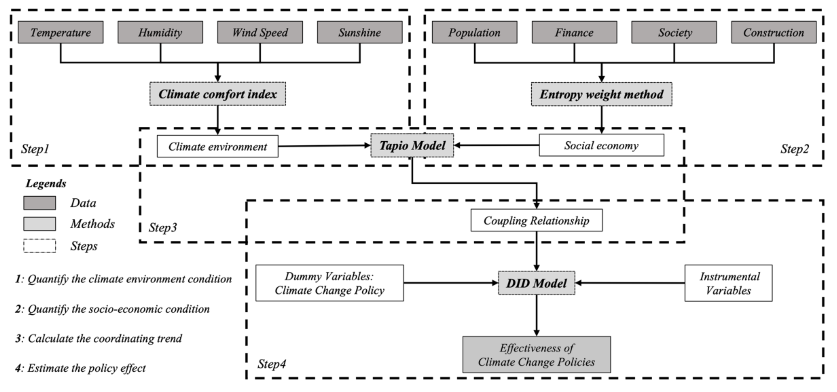
We designed a four-step research procedure to evaluate the value neutrality of policies related to ecological land protection and carbon emission reduction in a case study of Yangtze River Economic Belt, China (Figure 1).

In the first and second steps, we collected the climate and socio-economic data of the Yangtze River Economic Belt from 2008 to 2017 and quantified the level of climate and socio-economic conditions, respectively, based on the relative climate index and entropy weight method. In the third step, we calculated the coupling relationship between the climate and socio-economic conditions of the Yangtze River Economic Belt from 2008 to 2017 by using the Tapio model. In the fourth step, by sorting out the implementation status of climate change policies proposed in the white paper of “China’s policies and actions for addressing climate change” from 2008 to 2017, we estimated the impacts of mainstream climate change policies on the coupling degree between the subsystems of climate and economy by Difference-in-Difference (DID) model and further judged the value neutrality of policies related to low carbon and ecological land with various contents, objectives, and implementation strategies.

2.2. Data and Study Area

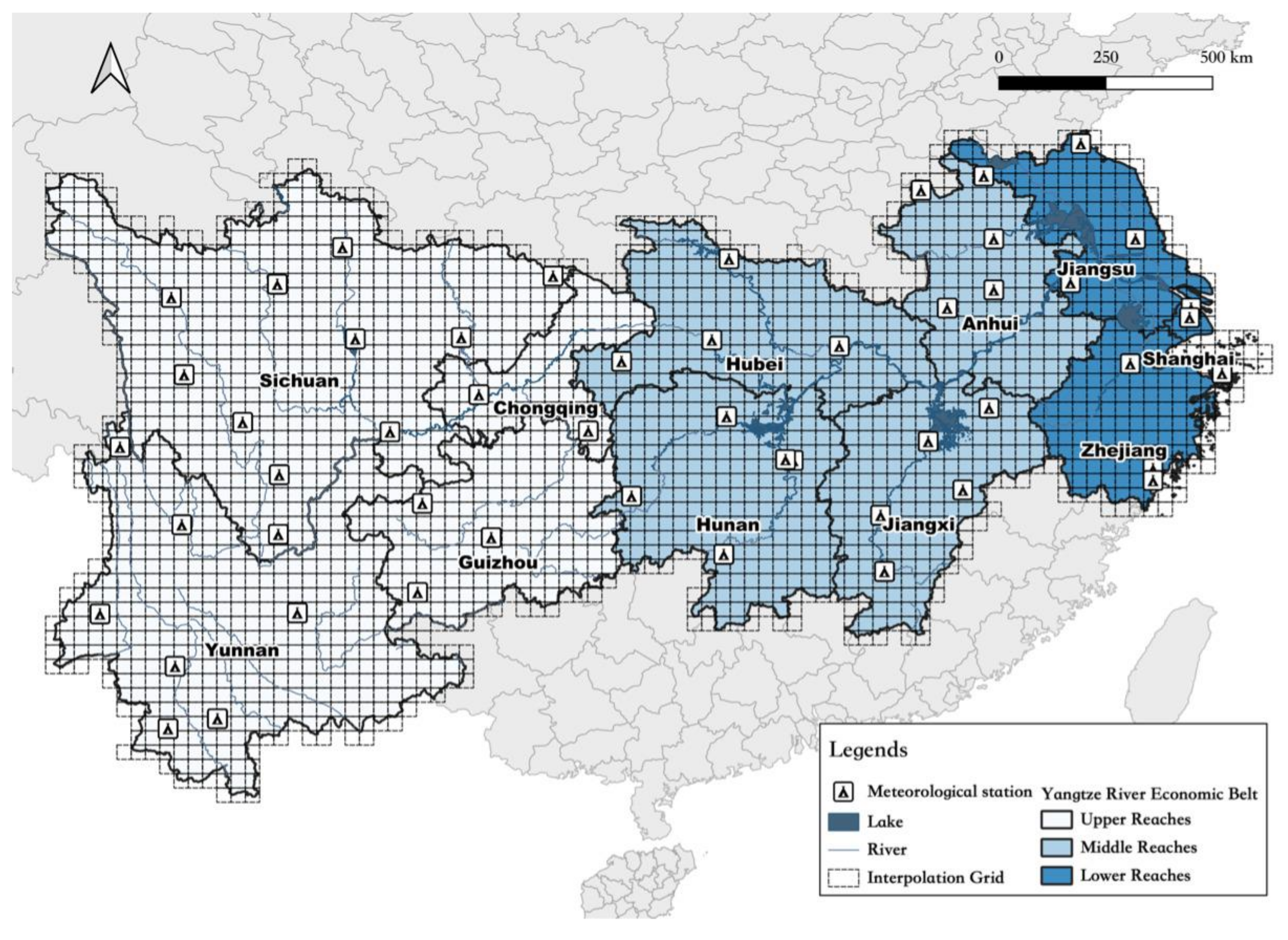
The case study was conducted at the Yangtze River Economic Belt, including 11 provinces (municipalities): Shanghai, Jiangsu, Zhejiang, Anhui, Jiangxi, Hubei, Hunan, Chongqing, Sichuan, Yunnan, and Guizhou.

This area was chosen for two reasons. First, the climate condition in this area is complex. The Yangtze River Economic Belt is across China (east–west direction) and covers three major climate zones. The case study in this region effectively eliminated the impact of climate zones on the accuracy of the analysis results. Second, the contradiction between climate and development is prominent in the Yangtze River Economic Belt [34]. While carrying out the policies of traffic system reconstruction and industrial structure optimization, the Chinese government also calls for the construction of this area as a demonstration zone for the protection and restoration of ecological environment systems [35]. Therefore, under the dual pressures of economic development and environmental governance, it is representative to study the coupling relationship between climate and economy at the Yangtze River Economic Belt.

The data regarding socio-economic conditions of the 11 provinces (or municipalities) in the Yangtze River Economic Belt was collected from the National Bureau of Statistics of China, which contained the annual data of urban population, finance, social life and space. The climate data came from the National Meteorological Science Data Center of China Meteorological Administration, including monthly temperature (°C), relative humidity (%), wind speed (m/s), and sunshine duration (h) at 48 meteorological stations within the Yangtze River Economic Belt.

It is worth mentioning that the spatial distribution of meteorological stations in the study area is uneven and the density is insufficient. The regional meteorological data outside the stations had to be estimated by certain mathematical methods from the observation values of adjacent stations [36]. In this work, we applied the Inverse Distance Weighted (IDW) method to interpolate the climate data [37]. The resolution of the interpolation grid was set as 0.03 longitude ×0.03 latitude according to the accuracy of original data, and a total of 2105 grids were constructed within the study area (Figure 2).

2.3. Relative Climate Index (RCI)

Referring to China’s local national standard of “DB46/T461-2018” [38], the Relative Climate Index, which is based mainly on the Temperature Humidity Index [39] and Wind Effect Index [40], was chosen to be the quantitative method of climate condition. The specific calculation formulas are shown in Formulas (1)–(3):

$$THI=1.8t +32 - 0.55(1 - h\left)\right(1.8t - 26)$$

(1)

$$K=8.55s - (10\sqrt{v}- v+10.45\left)\right(33 - t)$$

(2)

$$RCI=0.65THI+0.35K$$

(3)

where, THI denotes temperature humidity index; K denotes wind effect index; RCI denotes relative climate index; t denotes monthly average temperature (°C); h denotes monthly average relative humidity (%); v denotes monthly wind speed (m/s); s denotes monthly average sunshine duration (hour). The climate condition with the RCI value distributed in [−244.25, −24.5] is defined as suitable climate condition according to China’s local national standard “DB46/T461-2018” [38].

Using the Formulas (1)–(3), we could judge whether the monthly climate condition of the 2105 interpolation grids in the Yangtze River Economic Belt reaches the suitable level from 2008 to 2017. Furthermore, we calculated the length of the climate suitable period, the coverage of climate suitable zone, and the climate inequality of each province in the Yangtze River Economic Belt during the study period. The specific calculation formulas are as shown in Formulas (4)–(6):

$$LEN=\frac{{{\displaystyle \Sigma }}_{n=1}^k{l}_i^k}{n_i}$$

(4)

$$AREA=\frac{s_i}{n_i} \times 100\%$$

(5)

$$INEQ=\frac{1}{n_i}\underset{n_i=1}{\overset{n_i}{{\displaystyle \Sigma }}}ln(\frac{LEN}{l_i^k})$$

(6)

(The Theil entropy index was originally designed as a statistic to measure economic inequality. It has also been used to measure other social inequalities, such as apartheid [41]. Recently, it has also been introduced into the problem of uneven spatial distribution of climate and environmental indicators [42,43].) where, LEN denotes the length of climate suitable period (month); AREA denotes the coverage of climate suitable zone (%); INEQ denotes the Theil index of climate inequality [−1, 1]; i denotes the serial number of provinces; k denotes the serial number of interpolation girds; $l_i^k$ denotes the number of months with suitable climate in grid k of province i within 12 months; $s_i$ denotes the number of girds with suitable periods longer than 4 months in province i; $n_i$ denotes the total number of girds in province i.

2.4. Entropy Weight Method

Before measuring the coupling relationship between climate and socio-economic conditions under climate change policies, we need to further convert the calculation results of the climatic indicators (LEN, AREA and INEQ) and socio-economic data into indices reflecting the level of regional climate and socio-economic condition. In this study, we constructed an evaluation index system based on entropy weight method to form the climate index and economy index. Entropy weight method is an objective weighting method based on Shannon’s information entropy theory. In this method, we need to first judge the impact of each index on the evaluation target subjectively [44]. Formulas (7) and (8) present the method for standardizing the positive and negative indices, respectively.

Positive indicator (i.e., the larger the index value, the better the evaluation result):

$$X_{ij}{=X}_{ij}-min\left\{X_j\right\}/max\left\{X_j\right\}-min\left\{X_j\right\}$$

(7)

Negative indicator (i.e., the larger the index value, the worse the evaluation result):

$$X_{ij}=max\left\{X_j\right\}-X_{ij}/max\left\{X_j\right\}-min\left\{X_j\right\}$$

(8)

According to the variation degree of each indicator, the entropy weight of each indicator was calculated by using the information entropy, and then the weight of each indicator was modified by the entropy weight, so as to obtain the objective weight of each indicator [45].

In addition to the three climate indicators (LEN, AREA, and INEQ) mentioned in Section 2.2, we also selected 16 indicators to reflect the developing level of population, finance, social life, and space to construct evaluation index systems on climate and economy with the help of entropy weight method. The definition, information entropy, redundancy, and weight of 19 indicators are shown in

Table 1. Evaluation index systems of climate and socio-economic conditions.

System	Subsystem	Index	Description (Unit)	Effect	Entropy	Redundancy	Weight
Climate Condition (C)	Temporal	LEN	Length of periods with suitable climate (Month)	Positive	0.976	0.024	0.169
	Spatial	AREA	Coverage rate of areas with suitable climate (%)	Positive	0.891	0.109	0.767
	Inequality	INEQ	Theil Index (Range: [0, 1])	Negative	0.991	0.009	0.065
Socio-economic Condition (S)	Finance	FE	Fiscal expenditure per capita (10,000 RMB)	Positive	0.939	0.061	0.063
		RC	Resident consumption level per capita (RMB)	Positive	0.929	0.071	0.073
		GRP	Real GDP per capita (RMB)	Positive	0.943	0.057	0.059
		DI	Disposable and discretionary income (RMB)	Positive	0.925	0.075	0.078
	Population	PU	Proportion of urban population (%)	Positive	0.964	0.036	0.037
		SE	Social employees in enterprises, and institutions (%)	Positive	0.925	0.075	0.077
		PI	Private enterprises and individual employees (%)	Positive	0.912	0.088	0.091
		PD	Population density (Person/km2)	Positive	0.944	0.056	0.057
	Society	CU	Number of students in colleges and universities (Person/100,000 population)	Positive	0.975	0.025	0.026
		IT	Receiving international tourists (Millions of people)	Positive	0.939	0.061	0.062
		CP	Collection of public libraries (Volumes/10,000 population)	Positive	0.859	0.141	0.146
		MH	Medical and health institutions (Units/10,000 population)	Positive	0.961	0.039	0.040
	Space	BA	Urban built-up area (%)	Positive	0.956	0.044	0.046
		CL	Construction land (km2/10,000 population)	Positive	0.904	0.096	0.099
		GC	Green coverage rate of built-up area (%)	Positive	0.990	0.010	0.010
		RA	Road area (m2/person)	Positive	0.965	0.035	0.036

. Finally, using the entropy weight method, we quantified the climate and socio-economic conditions of the Yangtze River Economic Belt from 2008 to 2017 into two indicators: C (Climate condition) and S (Socio-economic condition).

2.5. Tapio Decoupling Model

The Tapio model, which had been widely used in the measurement of coupling relationships, was applied to measure the link between climate (C) and economy (S) [46]. The formula of the Tapio model is shown in Formula (9):

$$\phi =\frac{\Delta S_{t-1}/S}{\Delta C_{t-1}/C}$$

(9)

where, $\phi$ denotes the coupling coefficient between the climate and socio-economic condition; $\Delta S_{t-1}$ and $\Delta C_{t-1}$ denote the changes of climate and economy index from time t − 1 to t, respectively; S and C denote the climate condition and socio-economic condition of time t, respectively.

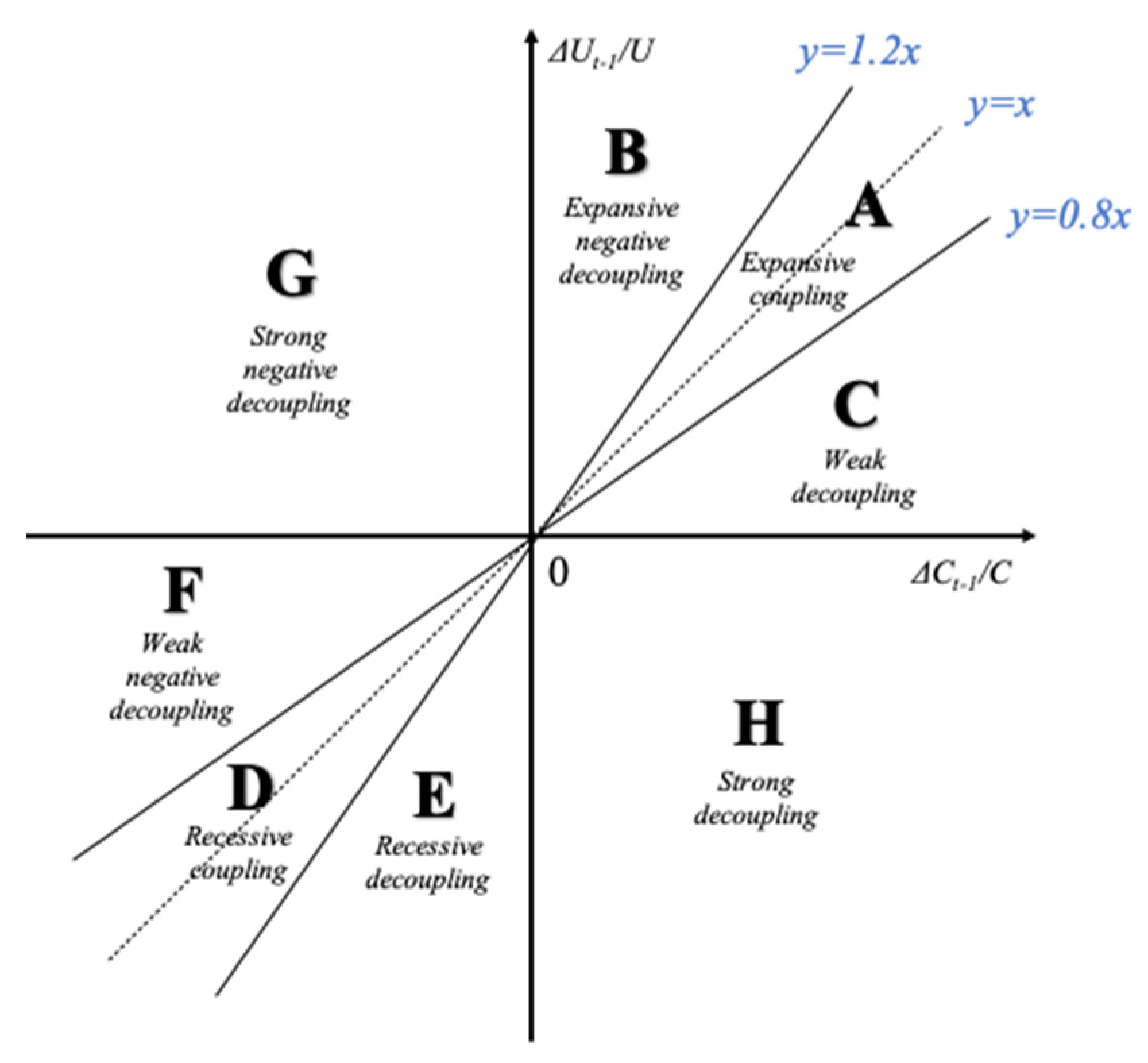
Furthermore, the coupling relationship between climate and socio-economic condition were divided into 8 types (A–H) according to signature of $\Delta S_{t-1}/S$ and $\Delta C_{t-1}/C$ and the value of $\phi$. According to Figure 3, when the change rate of socio-economic index and climate index are on the positive and negative sides respectively, the coupling coefficient is negative, and the two are in a strong decoupling relationship. When the change rate of socio-economic index (S) and climate index (C) are both located in the positive or negative side, the coupling coefficient is positive, and the type of coupling relationship depends on the distance from the coupling coefficient to 1. Specifically, when the coupling coefficient is distributed in [0.8, 1.2], climate and economy are in a state of coupling and are coordinated. When the coefficient is distributed in [0, 0.8], the greater the coupling coefficient, the stronger the coupling relationship. When the coefficient is distributed in [1.2, +∞], the smaller the coefficient, the stronger the coupling relationship. Moreover, the Jenks natural breaks optimization was applied to reclassify the coupling degree into integer grades of 1–10 according to the coupling coefficient between climate and socio-economic condition [47]. The reclassification results are shown in

Table 2. Classification rank of decoupling coefficient.

Coupling Degree	Value of φ	Definition
1	(−∞, −10.412]	Decoupling
2	(−10.412, −7.629]
3	(−7.629, −0.480]
4	(−0.480, 0]
5	(0, 0.156] and (30.091, +∞]	Relative coupling
6	(0.156, 0.289] and (19.743, 30.091]
7	(0.289, 0.424] and (3.237, 19.743]
8	(0.424, 0.520] and (1.832, 3.237]
9	(0.520, 0.8) and (1.2, 1.832]
10	[0.8, 1.2]	Coupling

Note: Jenks natural breaks optimization algorithm is applied to reclassify the coupling degree (value of φ).

. The higher the numerical grade of the coupling coefficient, the relationship between the variation trends of climate and socio-economic condition is more coordinated and sounder.

2.6. Difference-in-Difference Model

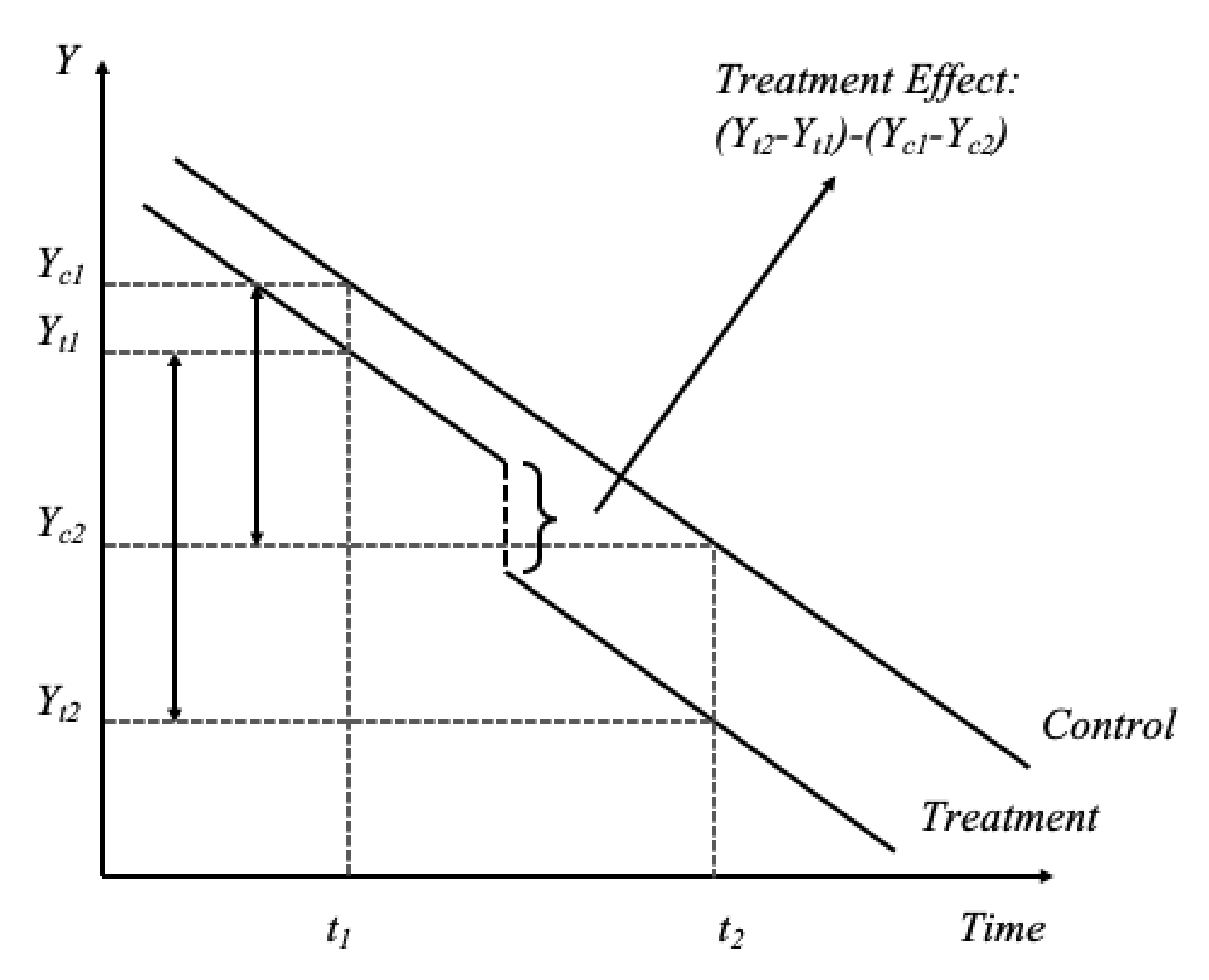
The Difference-in-Difference (DID) model was introduced to estimate the impact of climate change policies on the coupling relationship between regional climate condition and economic development and judge the value neutrality of polices. The DID model has been widely used in econometrics to quantitatively evaluate the implementation effect of public policies or projects [48,49]. DID is a quasi-experimental design that makes use of longitudinal data from treatment and control groups to obtain an appropriate counterfactual to estimate a causal effect. DID is typically used to estimate the effect of a specific intervention or treatment (such as a passage of law, enactment of policy, or large-scale program implementation) by comparing the changes in outcomes over time between a population that is enrolled in a program (the intervention group) and a population that is not (the control group) (see in Figure 4).

3. Results

3.1. Model Construction

In this work, the DID model was introduced to estimate the impact of policies and actions for addressing climate change proposed by the Chinese government from 2008 to 2017 on the coupling relationship between climate and economy within the white paper of “China’s policies and actions for addressing climate change” [50].

Specifically, the main contents regarding experimental sites of from 2008 to 2017 are shown in

Table 3. Major environmental policies and regarding experimental sites.

Policy	Main Contents	Starting Time	Experimental Sites
Low Carbon Province (LCP)	(1) Establishing the low-carbon industrial system; (2) Constructing the greenhouse gas emission dataset and management system	2010	Hubei, Yunnan
Low Carbon Community (LCC)	(1) Building zero-carbon architectures; (2) Utilizing new low-carbon energy sources; (3) Popularizing environmental-friendly building materials	2012	Chongqing
Ecological Civilization Construction (ECC)	(1) Improving forest coverage; (2) Increasing forest resource reserves; (3) Restoring the function of wetland ecosystem	2015	Guizhou
Ecosystem Protection and Restoration (EPR)	(1) Constructing national park (2) Strengthening forest and river ecosystem protection (Yangtze river) (3) Restoring biodiversity of forest and river ecosystem	2016	Sichuan

. From 2008 to 2017, four main climate change policies of Low Carbon Province (2010), Low Carbon Community (2012), Ecological Civilization Construction (2015), and Ecosystem Protection and Restoration (2016) had been proposed by the Ministry of Ecology and Environment of the People’s Republic of China in the main pilot sites of Hubei, Yunnan, Chongqing, Guizhou and Sichuan, which provided us with experimental conditions for a quasi-natural experiment to adopt the DID model. Among them, the first two policies are aimed at controlling regional carbon emissions, while the latter two are mainly committed to ecological land restoration, especially forests land. So far, this study constructed a two-way fixed-effect DID model as shown in Formula (10):

$$Y_{it}{=\beta }_0{+\beta }_1{Policy}_{it}{+\alpha X}_{it}{+t}_i{+s}_i{+\epsilon }_{it}$$

(10)

where, i and t denote the serial number of province and year, respectively. $Y_{it}$ denotes the dependent variables and represents the reclassification results of the coupling index between climate and socio-economic condition (Table 2). $Polic{y}_{it}$ denotes the dummy variable of the status of policy implementation. Since one province was chosen as the policy pilot site, the corresponding value of dummy variable $Polic{y}_{it}$ was taken as 1. Otherwise, the corresponding value was taken as 0. $t_i$ and $s_i$ denote the time and space fixed effect, respectively. $X_{it}$ denotes the instrumental variables including the value and change of climate and socio-economic condition indices. For the model, the signature and value of ${\beta }_1$ and the significance of $Polic{y}_{it}$ are crucial to the estimation of net effect of environmental policies. Specifically, the definitions and descriptive statistics of the variables included in the DID model are shown in

Table 4. Descriptive statistics of variables.

Variables	Definition	Min.	Mean	Max.
CCI	Change rate of climate condition index	−2.084	−0.108	0.633
CI	Climate condition index	0.430	1.008	1.623
CSEI	Change rate of socio-economic index	−0.268	0.096	0.421
SEI	Socio-economic index	0.086	0.288	0.799
CPR	Coupling index after reclassification	0	5.343	10
LCP	Dummy variable of policy of Low Carbon Province (0, 1)	0	0.162	1
LCC	Dummy variable of policy of Low Carbon Community (0, 1)	0	0.061	1
ECC	Dummy variable of policy of The Construction of Ecological Civilization (0, 1)	0	0.061	1
EPR	Dummy variable of policy of Ecosystem Protection and Restoration Program (0, 1)	0	0.000	1
PLA	Variable that determines whether an area is located in Plateau Climate Zone	0	0.091	1
SUB	Variable that determines whether an area is located in Subtropics Climate Zone	0	0.727	1
WAR	Variable that determines whether an area is located in Warm Climate Zone	0	0.182	1

.

In addition, considering that much attention has been drawn to the significant impact of climate zones on local climate and socio-economic conditions, the variables of PLA, SUB, and WAR were set to eliminate errors and improve the accuracy of the estimation. When the experimental sites are located in the plateau, subtropics, and warm climate zones, the values of variables PLA, SUB, and WAR were taken as 1, respectively.

3.2. Parametric Estimation

The results of global DID models are shown in

Table 5. Results of DID model.

Variables	(1)	(2)	(3)	(4)	(5)	(6)	(7)	(8)
LCP	3.111	2.611	—	—	—	—	—	—
	(1.848)	(1.596)
LCC	—	—	2.900	3.121 *	—	—	—	—
			(1.915)	(2.189)
ECC	—	—	—	—	3.567 *	3.725 **	—	—
					(2.381)	(2.639)
EPR	—	—	—	—	—	—	4.386 *	4.255 **
							(2.577)	(2.649)
CCI	—	1.181 **	—	1.289 **	—	1.313 **	—	1.222 **
		(3.510)		(3.897)		(4.025)		(3.776)
CI	—	0.233	—	0.107	—	0.035	—	0.216
		(0.456)		(0.222)		(0.074)		(0.444)
CSEI	—	−0.830	—	0.074	—	0.723	—	1.355
		(−0.262)		(0.023)		(0.267)		(0.509)
SEI	—	−0.413	—	0.249	—	0.553	—	−0.239
		(−0.239)		(0.174)		(0.394)		(−0.164)
(Intercept)	6.778 **	6.305 **	5.667 **	5.672 **	5.467 **	5.435 **	5.414 **	5.288 **
	(10.016)	(5.513)	(15.201)	(6.556)	(20.963)	(7.382)	(22.386)	(7.190)
R2	0.059	0.173	0.049	0.198	0.069	0.227	0.066	0.210

Note: * represents that 0.01 < p-value < 0.05; ** represents that 0 < p-value < 0.01; the number in brackets represents the T-value.

. In Table 5, models (1), (3), (5), and (7) were constructed to estimate the impacts of policies of Low Carbon Province, Low Carbon Community, Ecological Civilization Construction, and Ecosystem Protection and Restoration on the coupling development trend between climate and socio-economic conditions without adding instrumental variables, while models (2), (4), (6), and (8) were the same but included adding instrumental variables.

The outputs of the models indicated that the four main types of climate change policy all had a positive impact on the coupling development trend whether or not the instrumental variables were added. After adding the instrumental variables, the three policies (except Low Carbon Provinces) showed positive impacts on the coupling index at the significance level of 5%. Specifically, by observing the parametric estimation results of the models with better goodness-of-fit and instrumental variables, the coupling relationship between climate and socio-economic condition in experimental sites of Low Carbon Community, Ecological Civilization Construction, and Ecosystem Protection and Restoration were 3.121 (5% significance level), 3.725, and 4.235 units (1% significance level) higher than the control group.

These findings illustrated that the proportion of policies related to ecological lands that significantly improved the coupling degree between climate and socio-economic conditions of the pilot sites is more than that of carbon emission-related ones. Moreover, the average coupling degree between climate and socio-economic conditions in the pilot sites of ecological land policies was significantly increased by 3.99 units after policy implementation, which is 27.8% higher than that of carbon emission reduction policies.

In general, these two main results directly evidenced that the climate change policies aimed at improving the area and quality of ecological lands were more conducive to the coupling development of the climate–economy nexus than the policies focusing on restricting carbon emissions, which provides important enlightenment for the establishment of relevant environmental policies around the world.

3.3. Robustness Test: Climate Zones

The accuracy of the results of DID models was based on the premise that the control and experimental groups showed the same change trend [51]. Therefore, the verification of whether there was a similar change trend in the coupling degree between climate and socio-economic conditions within the research objects in this study was the priority issue. If there were significant differences in the coupling relationships between climate and socio-economic condition of cities in different climate zones, the conclusions drawn by DID model could not pass the robustness test. Therefore, the climate zone variables of PLA, SUB, and WAR were set in three additional DID models. The results of spatial robustness test are presented in

Table 6. Robustness test: climate zones.

Variables	(9)	(10)	(11)
PLA	−0.336	—	—
	(−0.455)
SUB	—	−0.275	—
		(−0.614)
WAR	—	—	0.563
			(1.063)
CCI	1.268 **	1.258 **	1.276 **
	(3.8726)	(3.806)	(3.872)
CI	0.250	0.144	0.197
	(0.502)	(0.297)	(0.412)
CSEI	0.683	0.549	0.566
	(0.253)	(0.203)	(0.211)
SEI	−0.406	−0.294	−0.658
	(−0.277)	(−0.207)	(−0.450)
(Intercept)	5.310 **	5.565 **	5.315 **
	(7.039)	(6.373)	(7.086)
R2	0149	0.150	0.157

Note: ** represents that 0 < p-value < 0.01; the number in brackets represents the T-value.

.

In Table 6, models (9)–(11) were constructed to verify the differences in the impact of climate change policies on coupling development trends between climate and socio-economic condition in plateau, subtropics, and warm climate zones, respectively. The results showed that the significance levels of PLA, SUB, and WAR were all greater than 5% and there was no significant difference in the coefficients, significance of other instrumental variables, or the goodness-of-fit between models (9)–(11) and (1)–(8). This further indicated that no matter which climate zone the pilot site was located in, there was no statistical difference in the coupling development trend between climate and economy at the provincial level. These outputs documented that the coupling coefficients of pilot sites involved in the study showed a common change trend. Therefore, the estimated results of DID models in Table 5 passed the common trend test.

3.4. Robustness Test: Time Effects

In addition, if the outputs of DID models are robust, which means the differences in coupling coefficients of the research objects were caused by the promulgation of climate change policies, the significant differences in climate and socio-economic condition between the pilot sites, and the control sites should only appear before and after the time points when the policies are launched. Therefore, this study further assumed that the first promulgation time of policies in each pilot province of the Yangtze River Economic Belt is 1 and 2 years ahead of schedule, and the time effect of DID models was verified by judging whether the coefficients of virtual dummy variables were significantly positive. The results of temporal robustness tests are presented in

Table 7. Robustness test: time effects.

Variables	(12)	(13)	(14)	(15)	(16)	(17)
POLICY A1	1.901	—	2.412	—	2.691	—
	(1.1.50)		(1.745)		(1.877)
POLICY A2	—	−1.503	—	1.964	—	1.687
		(−0.686)		(1.428)		(1.188)
DCL	1.286 **	1.207 **	1.340 **	1.212 **	1.360 **	1.386 **
	(3.761)	(3.556)	(3.847)	(3.683)	(4.072)	(3.934)
CL	1.622	0.127	0.014	0.076	0.225	0.220
	(0.330)	(0.257)	(0.029)	(0.155)	(0.456)	(0.439)
DURB	0.597	0.202	0.184	−0.052	0.169	0.367
	(0.190)	(0.064)	(0.064)	(−0.017)	(0.061)	(0.123)
URB	0.077	−0.007	0.427	0.246	0.032	0.057
	(0.053)	(−0.005)	(0.299)	(0.172)	(0.022)	(0.038)
(Intercept)	5.441 **	5.490 **	5.575 **	5.572 **	5.512 **	5.517 **
	(5.815)	(4.941)	(7.213)	(6.912)	(7.324)	(7.065)
R2	0.164	0.157	0.194	0.180	0.192	0.172

Note: ** represents that 0 < p-value < 0.01; the number in brackets represents the T-value.

.

In Table 7, model (12), (14), and (16) were constructed to estimate the impacts of climate change policies in cases that the policies were launched 1 year in advance, while model (13), (15), and (17) represent the results of 2 years in advance. The results presented in Table 7 indicated that the policies did not significantly affect the coupling development trend in the hypothetical scenario since the significance levels of coefficients POLICY A1 and POLICY A2 in model (12)–(17) were all greater than the threshold value of 5%. These results further illustrated that the impacts of climate change policies on the coupling development trend only existed before and after the promulgation of each policy, and the temporal robustness of DID models was verified, as well.

In summary, the effect of climate change policies on coupling the development trend of climate–economy nexus only occurred after the implementation of the policy. Therefore, the main results of this study on the value neutrality in China’s environmental policies are robust and reliable.

4. Discussions

The empirical results in Section 3 indicated that China’s climate change policies, except for Low Carbon Provinces, effectively promoted the coupling trend between climate and socio-economic conditions in China, showing strong value neutrality. However, the policies with different content and objectives showed a significant difference in the impacts on the environment–development nexus. Specifically, the environmental policies targeting improving the area and quality of ecological lands with forests as the core (Ecological Civilization Construction and Ecosystem Protection and Restoration) are more conducive to the coupling development of the environment–development nexus and show stronger value neutrality than the policies focusing on restricting carbon emissions (Low Carbon Provinces and Low Carbon Community). There are two possible explanations for this.

On the one hand, the more specific implementation contents might be the key to the stronger value neutrality of ecological land policies. Within the case study area, the carbon emission policies proposed by the provincial governments of China didn’t include the implementation path to achieve the low-carbon goals. The governments of Hubei and Yunnan province only take the establishment of the low-carbon industrial system and the construction of greenhouse gas emission dataset as the core and objectives of carbon emission reduction policies. This result ties well with recent studies on China’s policy of carbon emission. It has been demonstrated that proposing targets for industrial transformation and developing environmental plans is not effective in moderating regional carbon emission levels. Starting with the carbon trading process and improving the core technology of carbon dioxide emission are reasonable approaches to deal with climate change [52,53]. In contrast, the policies related to ecological land protection stipulated specific objects and strategies to optimize the area and quality of forests, water, and other types of land-use with outstanding ecosystem optimization and restoration functions. Improving the regional forest coverage, forest reserves, and establishing national parks, which could comprehensively improve the biodiversity and ecological vitality of regional forest and water ecosystems, were recognized as the three main approaches to deal with the negative impact of the dramatic climate change. This is also reported in Sotirov and Storch’s investigation on European forest policies; the objectives, tools, and practices of forest policies in France, Germany, the Netherlands, and Sweden have demonstrated effectiveness and stability over the past decades. The implementation guidelines of these policies, which directly address timber production, timber harvesting, sustainable forest management, and biodiversity conservation, are an important guarantee of their effectiveness [54,55].

On the other hand, the stronger value neutrality of climate change policies related to ecological land protection might be the result of the upgrade in implementation strategy of China’s environmental policies and the promotion of citizens’ environmental awareness. Carbon emission reduction policies were mainly released before 2012, while the main content of climate change response policies after 2015 turned out to be ecological land protection. Tang and Chen [56] summarized that Chinese central government regarded environmental protection as the main task in China’s future growth after 2015, and the motivation of local government’s environmental governance was also increasing. In addition, the continuous improvement of public attention to environmental protection and the rapid development of new media had also promoted the rapid increase of Chinese citizens’ ecological protection awareness, which has greatly promoted the efficient implementation of environmental policies in recent years [57]. As a result, the climate change policies related to ecological lands launched after 2012 could effectively promote the coupling development trend between climate and socio-economic conditions. Overall, our assumptions on the link between environmental awareness and value neutrality of climate change policies are in accordance with findings reported in previous literature. As the environmental policies of urban residents improve, the regional environmental quality and the efficiency of environmental policy implementation will increase in parallel. In addition to this, environmental awareness and environmental policy have a mutual influence mechanism with each other [58,59,60]. Moreover, since the impact of the upgrading of citizens’ environmental awareness on the implementation efficiency of environmental policies is sometimes ignored, environmental education and climate protection publicity should also be carried out together with the proposal of environmental policies.

In addition, it is important to highlight that although the empirical results of this study suggest the climate change policies aimed at improving the area and quality of ecological lands were more conducive to the coupling development of the climate–economy nexus than the policies focusing on restricting carbon emissions, the shortcomings and expertise of both types of climate change policies had also been widely reported in related literature. Specifically, climate change policies related to ecological land run the risk of creating conflicts of interest in biological resources while addressing the negative impacts of climate change by restoring regional ecosystems and biodiversity, especially in the Pacific Northwest [61]. While the policies related to carbon emissions are seen as having a negative economic impact in the short term, they promote the use of natural gas and renewable energy and the transformation of the energy structure in the long term [62].

5. Conclusions and Policy Implications

In this paper, we proposed a quantitative framework to measure the effectiveness of climate change policies and compared the value neutrality of policies aiming at reducing carbon emissions and optimizing forests. Taking the Yangtze River Economic Belt in China as an example, we clarified the impact of climate change policies on the coupling development trend between regional climate and socio-economic conditions and judged the value neutrality of these policies.

The results showed that the proportion of policies related to ecological lands that significantly improved the coupling degree between climate and socio-economic conditions of the pilot sites is more than that of carbon emission related ones. Moreover, the average coupling degree between climate and socio-economic conditions in the pilot sites of ecological land policies was significantly increased by 3.99 units after policy implementation, which is 27.8% higher than that of carbon emission reduction policies. Together, these findings confirmed that the climate change policies aimed at improving the area and quality of ecological lands were more conducive to the coupling development of the climate–economy nexus than the policies focusing on restricting carbon emissions.

Based on the above conclusions, we put forward the following policy implications for the Chinese government. Firstly, the coupling index between climate and socio-economic conditions among policy pilot sites before and after policy implementation should be considered as the indicators of policy effectiveness evaluation. Compared with the direct statistics of environmental and economic data, coupling relationship is more conductive to judge the long-tern comprehensive impact of policy implementation on the regional climate–economy nexus and evaluate the value neutrality within the climate change policies. Secondly, the objectives and implementation strategies of climate policies should be specific. For example, the policies aiming at reducing carbon emissions could take optimizing the carbon cycle system of new building materials, improving the utilization rate of low-carbon energy in the industrial system, and actively promoting the utilization rate of public transport as the primary implementation strategies. In general, taking the coupling relationship between economic and environmental systems in pilot regions into consideration and refining specific measures for policy implementation are summarized as two potential improvement directions for global future policy responses for climate change from this pilot study.

The main academic contribution of this study is to design a new evaluation framework for the value neutrality of climate change policies from the perspective of dynamic coupling, and quantitatively compare the difference in the effectiveness of the current mainstream climate change policies. It brings a new perspective and methodology for the future evaluation of environmental policies and provides a quantitative basis for the formulation and implementation of future climate change policies.

Due to the limitations in data and methods to measure the implementation mode of environmental policies, the relationship between implementation mode and efficiency of policies was not included in the regression models. This is the main deficiency of this paper. Therefore, clarifying the impact mechanism of different implementation modes on the effectiveness of environmental policies will be the future direction of this study.

References

- Watson, R.T.; Zinyowera, M.C.; Moss, R.H.; Dokken, D.J. The Regional Impacts of Climate Change; IPCC: Geneva, Switzerland, 1998. [Google Scholar]
- Tompkins, E.L.; Adger, W.N. Does Adaptive Management of Natural Resources Enhance Resilience to Climate Change? Ecol. Soc. 2004, 9, 10. [Google Scholar] [CrossRef]
- McMichael, A.J.; Woodruff, R.E.; Hales, S. Climate Change and Human Health: Present and Future Risks. Lancet 2006, 367, 859–869. [Google Scholar] [CrossRef]
- Taylor, R.G.; Scanlon, B.; Döll, P.; Rodell, M.; Van Beek, R.; Wada, Y.; Longuevergne, L.; Leblanc, M.; Famiglietti, J.S.; Edmunds, M.; et al. Ground Water and Climate Change. Nat. Clim. Chang. 2013, 3, 322–329. [Google Scholar] [CrossRef] [Green Version]
- Malmsheimer, R.W.; Heffernan, P.; Brink, S.; Crandall, D.; Deneke, F.; Galik, C.; Gee, E.; Helms, J.A.; McClure, N.; Mortimer, M.; et al. Forest Management Solutions for Mitigating Climate Change in the United States. J. For. 2008, 106, 115–173. [Google Scholar]
- Colding, J. ‘Ecological Land-Use Complementation’ for Building Resilience in Urban Ecosystems. Landsc. Urban Plan. 2007, 81, 46–55. [Google Scholar] [CrossRef]
- Peng, J.; Zhao, M.; Guo, X.; Pan, Y.; Liu, Y. Spatial-Temporal Dynamics and Associated Driving Forces of Urban Ecological Land: A Case Study in Shenzhen City, China. Habitat Int. 2017, 60, 81–90. [Google Scholar] [CrossRef]
- Chuai, X.; Huang, X.; Wu, C.; Li, J.; Lu, Q.; Qi, X.; Zhang, M.; Zuo, T.; Lu, J. Land Use and Ecosystems Services Value Changes and Ecological Land Management in Coastal Jiangsu, China. Habitat Int. 2016, 57, 164–174. [Google Scholar] [CrossRef]
- Hegerl, G.C.; voN SToRcH, H.; Hasselmann, K.; Santer, B.D.; Cubasch, U.; Jones, P.D. Detecting Greenhouse-Gas-Induced Climate Change with an Optimal Fingerprint Method. J. Clim. 1996, 9, 2281–2306. [Google Scholar] [CrossRef] [Green Version]
- Smith, S.M.; Lowe, J.A.; Bowerman, N.H.; Gohar, L.K.; Huntingford, C.; Allen, M.R. Equivalence of Greenhouse-Gas Emissions for Peak Temperature Limits. Nat. Clim. Chang. 2012, 2, 535–538. [Google Scholar] [CrossRef]
- Martinez, L.H. Post Industrial Revolution Human Activity and Climate Change: Why the United States Must Implement Mandatory Limits on Industrial Greenhouse Gas Emissions. J. Land Use Environ. Law 2005, 403–421. [Google Scholar]
- Manabe, S. Role of Greenhouse Gas in Climate Change. Tellus A Dyn. Meteorol. Oceanogr. 2019, 71, 1620078. [Google Scholar] [CrossRef] [Green Version]
- Wang, Q.; Wang, S.; Li, R. Determinants of decoupling economic output from carbon emission in the transport sector: A comparison study of four municipalities in China. Int. J. Environ. Res. Public Health 2019, 16, 3729. [Google Scholar] [CrossRef] [Green Version]
- Dhakal, S. Urban Energy Use and Carbon Emissions from Cities in China and Policy Implications. Energy Policy 2009, 37, 4208–4219. [Google Scholar] [CrossRef]
- Andersson, F.N. International Trade and Carbon Emissions: The Role of Chinese Institutional and Policy Reforms. J. Environ. Manag. 2018, 205, 29–39. [Google Scholar] [CrossRef]
- Agrell, P.J.; Stam, A.; Fischer, G.W. Interactive Multiobjective Agro-Ecological Land Use Planning: The Bungoma Region in Kenya. Eur. J. Oper. Res. 2004, 158, 194–217. [Google Scholar] [CrossRef]
- Tan, Y.; Wu, C.; Wang, Q.; Zhou, L.; Yan, D. The Change of Cultivated Land and Ecological Environment Effects Driven by the Policy of Dynamic Equilibrium of the Total Cultivated Land. J. Nat. Resour. 2005, 20, 727–734. [Google Scholar]
- Howarth, R.B. An Overlapping Generations Model of Climate-Economy Interactions. Scand. J. Econ. 1998, 100, 575–591. [Google Scholar] [CrossRef]
- Dell, M.; Jones, B.F.; Olken, B.A. What Do We Learn from the Weather? The New Climate-Economy Literature. J. Econ. Lit. 2014, 52, 740–798. [Google Scholar] [CrossRef] [Green Version]
- Wang, Q.; Jiang, R. Is China’s Economic Growth Decoupled from Carbon Emissions? J. Clean. Prod. 2019, 225, 1194–1208. [Google Scholar] [CrossRef]
- Kameyama, Y.; Morita, K.; Kubota, I. Finance for Achieving Low-Carbon Development in Asia: The Past, Present, and Prospects for the Future. J. Clean. Prod. 2016, 128, 201–208. [Google Scholar] [CrossRef]
- Wang, S.; Van Kooten, G.C.; Wilson, B. Mosaic of Reform: Forest Policy in Post-1978 China. For. Policy Econ. 2004, 6, 71–83. [Google Scholar] [CrossRef]
- Li, L.; Lei, Y.; Wu, S.; He, C.; Yan, D. Study on the Coordinated Development of Economy, Environment and Resource in Coal-Based Areas in Shanxi Province in China: Based on the Multi-Objective Optimization Model. Resour. Policy 2018, 55, 80–86. [Google Scholar] [CrossRef]
- Nunes, P.; Pinheiro, F.; Brito, M.C. The Effects of Environmental Transport Policies on the Environment, Economy and Employment in Portugal. J. Clean. Prod. 2019, 213, 428–439. [Google Scholar] [CrossRef]
- Azar, C.; Dowlatabadi, H. A Review of Technical Change in Assessment of Climate Policy. Annu. Rev. Energy Environ. 1999, 24, 513–544. [Google Scholar] [CrossRef]
- Victor, D. Climate Change: Embed the Social Sciences in Climate Policy. Nat. News 2015, 520, 27. [Google Scholar] [CrossRef] [Green Version]
- Li, Q.; Hu, H.; Luo, H.; Lin, L.; Shi, Y.; Zhang, Y.; Zhou, L. Two-Way Coupling Relationship between Economic Growth and Environmental Pollution-Regional Difference Analysis Based on PVAR Model. Acta Sci. Circumstantiate 2015, 6, 1875–1886. [Google Scholar]
- Dinda, S. Environmental Kuznets Curve Hypothesis: A Survey. Ecol. Econ. 2004, 49, 431–455. [Google Scholar] [CrossRef] [Green Version]
- Nordhaus, W.D. The ‘dice’ Model: Background and Structure of a Dynamic Integrated Climate-Economy Model of the Economics of Global Warming; Cowles Foundation for Research in Economics, Yale University: New Haven, CT, USA, 1992. [Google Scholar]
- Nordhaus, W.D.; Boyer, J. Warming the World: Economic Models of Global Warming; MIT Press: Cambridge, MA, USA, 2000. [Google Scholar]
- Smets, F.; Wouters, R. An Estimated Dynamic Stochastic General Equilibrium Model of the Euro Area. J. Eur. Econ. Assoc. 2003, 1, 1123–1175. [Google Scholar] [CrossRef] [Green Version]
- Hassani-Mahmooei, B.; Parris, B.W. Climate Change and Internal Migration Patterns in Bangladesh: An Agent-Based Model. Environ. Dev. Econ. 2012, 17, 763–780. [Google Scholar] [CrossRef]
- Toth, F. Coupling climate and economic dynamics: Recent achievements and unresolved problems. In The Coupling of Climate and Economic Dynamics; Springer: Berlin/Heidelberg, Germany, 2005. [Google Scholar]
- Chen, Y.; Zhang, S.; Huang, D.; Li, B.-L.; Liu, J.; Liu, W.; Ma, J.; Wang, F.; Wang, Y.; Wu, S.; et al. The Development of China’s Yangtze River Economic Belt: How to Make It in a Green Way. Sci. Bull. 2017, 62, 648–651. [Google Scholar] [CrossRef] [Green Version]
- Luo, Q.; Luo, L.; Zhou, Q.; Song, Y. Does China’s Yangtze River Economic Belt Policy Impact on Local Ecosystem Services? Sci. Total. Environ. 2019, 676, 231–241. [Google Scholar] [CrossRef]
- De Caceres, M.; Martin-StPaul, N.; Turco, M.; Cabon, A.; Granda, V. Estimating Daily Meteorological Data and Downscaling Climate Models over Landscapes. Environ. Model. Softw. 2018, 108, 186–196. [Google Scholar] [CrossRef]
- Chen, F.-W.; Liu, C.-W. Estimation of the Spatial Rainfall Distribution Using Inverse Distance Weighting (IDW) in the Middle of Taiwan. Paddy Water Environ. 2012, 10, 209–222. [Google Scholar] [CrossRef]
- Hainan, A. Market Regulation of Meteorological Index Ratings (RCI): Evaluation on Climate Comfort Degree; AMR: Hainan, China, 2018. [Google Scholar]
- Steadman, R.G. The Assessment of Sultriness. Part I: A Temperature-Humidity Index Based on Human Physiology and Clothing Science. J. Appl. Meteorol. Climatol. 1979, 18, 861–873. [Google Scholar] [CrossRef] [Green Version]
- Siple, P.A.; Passel, C.F. Measurements of Dry Atmospheric Cooling in Subfreezing Temperatures. Proc. Am. Philos. Soc. 1945, 89, 177–199. [Google Scholar] [CrossRef]
- Conceição, P.; Ferreira, P. The Young Person’s Guide to the Theil Index: Suggesting Intuitive Interpretations and Exploring Analytical Applications. SSRN 2000. [Google Scholar] [CrossRef] [Green Version]
- Tian, Q.; Zhao, T.; Yuan, R. An Overview of the Inequality in China’s Carbon Intensity 1997–2016: A Theil Index Decomposition Analysis. Clean Technol. Environ. Policy 2021, 23, 1581–1601. [Google Scholar] [CrossRef]
- Liu, T.; Pan, W. The Regional Inequity of CO2 Emissions per Capita in China. Int. J. Econ. Financ. 2017, 9, 228–241. [Google Scholar] [CrossRef] [Green Version]
- Mon, D.-L.; Cheng, C.-H.; Lin, J.-C. Evaluating Weapon System Using Fuzzy Analytic Hierarchy Process Based on Entropy Weight. Fuzzy Sets Syst. 1994, 62, 127–134. [Google Scholar] [CrossRef]
- Zou, Z.-H.; Yi, Y.; Sun, J.-N. Entropy Method for Determination of Weight of Evaluating Indicators in Fuzzy Synthetic Evaluation for Water Quality Assessment. J. Environ. Sci. 2006, 18, 1020–1023. [Google Scholar] [CrossRef]
- Tapio, P. Towards a Theory of Decoupling: Degrees of Decoupling in the EU and the Case of Road Traffic in Finland between 1970 and 2001. Transp. Policy 2005, 12, 137–151. [Google Scholar] [CrossRef] [Green Version]
- Chen, J.; Yang, S.; Li, H.; Zhang, B.; Lv, J. Research on Geographical Environment Unit Division Based on the Method of Natural Breaks (Jenks). Int. Arch. Photogramm. Remote Sens. Spat. Inf. Sci. 2013, 3, 47–50. [Google Scholar] [CrossRef] [Green Version]
- Conley, T.G.; Taber, C.R. Inference with “Difference in Differences” with a Small Number of Policy Changes. Rev. Econ. Stat. 2011, 93, 113–125. [Google Scholar] [CrossRef] [Green Version]
- Donald, S.G.; Lang, K. Inference with Difference-in-Differences and Other Panel Data. Rev. Econ. Stat. 2007, 89, 221–233. [Google Scholar] [CrossRef]
- Wang, W.; Zheng, G.; Pan, J. China’s Climate Change Policies; Routledge: London, UK, 2013. [Google Scholar]
- Liu, R.; Zhao, R. Does National High–Tech Zone Promote Regional Economy. Manag. World 2015, 8, 30–38. [Google Scholar]
- Xuan, D.; Ma, X.; Shang, Y. Can China’s policy of carbon emission trading promote carbon emission reduction? J. Clean. Prod. 2020, 270, 122383. [Google Scholar] [CrossRef]
- Li, W.; Lu, C.; Ding, Y.; Zhang, Y.W. The impacts of policy mix for resolving overcapacity in heavy chemical industry and operating national carbon emission trading market in China. Appl. Energy 2017, 204, 509–524. [Google Scholar] [CrossRef]
- Sotirov, M.; Storch, S. Resilience through policy integration in Europe? Domestic forest policy changes as response to absorb pressure to integrate biodiversity conservation, bioenergy use and climate protection in France, Germany, The Netherlands and Sweden. Land Use Policy 2018, 79, 977–989. [Google Scholar] [CrossRef]
- Sotirov, M.; Winkel, G.; Eckerberg, K. The coalitional politics of the European Union’s environmental forest policy: Biodiversity conservation, timber legality, and climate protection. Ambio 2017, 50, 2153–2167. [Google Scholar] [CrossRef] [PubMed]
- Xiao, T.; Wei-wei, C. Motivation, Incentive and Information: The Theoretical Framework and Typological Analysis of China’s Environmental Policy Implementation. J. Chin. Acad. Gov. 2017, 1, 76–81. [Google Scholar]
- Wang, R.; Qi, R.; Cheng, J.; Zhu, Y.; Lu, P. The Behavior and Cognition of Ecological Civilization among Chinese University Students. J. Clean. Prod. 2020, 243, 118464. [Google Scholar] [CrossRef]
- Galli, A.; Iha, K.; Pires, S.M.; Mancini, M.S.; Alves, A.; Zokai, G.; Wackernagel, M. Assessing the ecological footprint and biocapacity of Portuguese cities: Critical results for environmental awareness and local management. Cities 2020, 96, 102442. [Google Scholar] [CrossRef]
- Calculli, C.; D’Uggento, A.M.; Labarile, A.; Ribecco, N. Evaluating people’s awareness about climate changes and environmental issues: A case study. J. Clean. Prod. 2021, 324, 129244. [Google Scholar] [CrossRef]
- Geng, M.M.; He, L.Y. Environmental Regulation, Environmental Awareness and Environmental Governance Satisfaction. Sustainability 2021, 13, 3960. [Google Scholar] [CrossRef]
- Winkel, G. When the pendulum doesn’t find its center: Environmental narratives, strategies, and forest policy change in the US Pacific Northwest. Glob. Environ. Chang. 2014, 27, 84–95. [Google Scholar] [CrossRef]
- Li, R.; Su, M. The role of natural gas and renewable energy in curbing carbon emission: Case study of the United States. Sustainability 2017, 9, 600. [Google Scholar] [CrossRef] [Green Version]