
Spatiotemporal Simulation of Green Space by Considering Socioeconomic Impacts Based on A SD-CA Model

1
School of Landscape Architecture, Beijing Forestry University, No. 35, Tsinghua East Road, Haidian District, Beijing 100083, China
2
School of Economics and Management, Beijing Forestry University, No. 35, Tsinghua East Road, Haidian District, Beijing 100083, China
*
Author to whom correspondence should be addressed.
Forests 2021, 12(2), 202; https://0-doi-org.brum.beds.ac.uk/10.3390/f12020202
Submission received: 25 December 2020
/
Revised: 5 February 2021
/
Accepted: 6 February 2021
/
Published: 10 February 2021
(This article belongs to the Special Issue Landscape and Urban Planning-Sustainable Forest Development)
Abstract
:Green space is an important part of composite urban spatial systems. Therefore, reasonable planning strategies based on scientifically sound predictions of temporal and spatial changes in green space are critical for maintaining urban ecological environments, ensuring the health of residents, and maintaining social stability. However, existing forecasting models discount the impacts of urban social economy on green space. To address this gap, we constructed a system dynamics and cellular automata (SD-CA) coupling model that integrated the socioeconomic system and generated multiple scenarios. The results showed that at the current pace of socioeconomic development, Beijing’s central district will experience an overall reduction in green space and a decline in its integrity and diversity by 2035. If the population of this area reaches 9.29 million by 2035 and the GDP maintains an average growth rate of 6.1%, the areas of various land types will exhibit little change by 2035, and green space will be optimized to a certain extent. However, if the study area’s population decreases to 8.59 million by 2035 and the average GDP growth rate drops to 4.9%, the fragmentation, connectivity, and diversity index of green space will all increase significantly by 2035, and green space will be clearly optimized. We propose scientifically grounded strategies for maximizing the ecological functions and economic benefits of green space through optimized green space patterns, considered from a policy-oriented perspective of promoting socioeconomic development.
1. Introduction
Healthy and well-managed urban green spaces contribute significantly to the quality of life of urban residents [1,2,3,4]. However, rapid socioeconomic development and ongoing urban expansion are resulting in the continuous occupation of urban green space and a consequent decrease in green space, which in turn increases the heat island effect and air pollution [5,6,7,8]. Thus, there is an urgent need to optimize patterns of urban green space and promote coordinated socioeconomic and urban green space development to meet social needs and promote environmental sustainability [9,10]. The relationship between the area of urban green space and socioeconomic development has attracted considerable scholarly attention [11]. Such studies were initiated in the 1980s and mainly focused on urban growth and ecological security [12,13]. Research on green space in landscape architecture and related disciplines focused on the evolution of spatial patterns [14], landscape patterns [15,16], service functions [17], and planning practices [18]. Current research on this topic has mainly focused on the social, economic, and ecological benefits of green space. Studies conducted on its social benefits have shown that it promotes human activities and communication and significantly improves people’s happiness levels [19]. The economic benefits of urban green space relate to its critical role in enhancing the environment and environmental conveniences, thus expanding the real estate market and contributing significantly to sustainable economic development [20]. Studies have also highlighted the ecological benefits of green spaces, which can help to purify polluted air [21,22], reduce the urban heat island effect [23,24], protect water resources from pollution [25], and maintain biodiversity [26,27,28]. Zhang et al. (2013) found that residential, demographic, and socioeconomic factors significantly influence individuals’ preferences regarding leisure and entertainment in urban parks [29]. In sum, a very close relationship exists between urban green space and socioeconomic development [30].
From a methodological standpoint, a variety of approaches have been used to model the spatial process [31], including potential models [12], the Markov Chain [32], and spatial logistic regression [33]. Additionally, remotely sensed data with a medium spatial resolution, such as Landsat Thematic Mapper images, have been used to explore spatial patterns and changes in urban green space [34,35]. There is a growing body of literature on applications of the cellular automata (CA) and system dynamics (SD) models in studies on land-use changes [36,37,38]. The CA model, which is a dynamic model with powerful spatial computing capabilities, can effectively simulate complex self-organization phenomena [39]. Cláudia et al. (2003) developed a CA model to explore the spatiotemporal characteristics of land-use changes in medium-sized cities and towns in the western part of Sao Paulo state in Brazil based on an analysis of changes in the economy and land-use patterns of this region [40]. Li and Yeh (2000) extended the CA model by integrating it with geographic information systems (GIS) to facilitate planners in designing urban forms that could contribute to sustainable development [41]. However, this “bottom-up” model is not suitable for assessing macro socioeconomic factors that affect regional land-use changes [42]. Some researchers have attempted to integrate the CA model with an economic model to resolve this issue. Barredo et al. (2003) integrated land-use factors with the CA approach to model future urban land-use scenarios, the results of the model have been tested using the fractal dimension and comparison matrix methods [43]. Caruso et al. (2009) developed a theoretical model of residential growth that emphasized the path-dependent nature of urban sprawl patterns [44]. The model was based on a monocentric urban economic model in which the CA approach was used to introduce endogenous neighborhood effects.
In addition, an SD model enables the expression of nonlinear causal loop relationships, information feedback, and complex dynamic problems that change over time [45]. Li et al. (2015) used an SD model to assess Beijing’s forest ecological security under different scenarios, providing a basis for decision making aimed at the overall improvement of forest conditions [46]. Wang et al. (2014) used an SD model in a quantitative evaluation of the utilization efficiency of China’s existing marine functional zone [47]. Guo et al. (2001) and Zhang (1997) contended that the SD model, as a “top-down” model, is unable to handle spatial data and adequately describe the spatial process of land use [48,49].
In general, research on the relationship between urban green space and socioeconomic development has advanced considerably. However, given that this field is still evolving, some gaps remain. First, studies on the ecological conservation of green space often take a single ecological element as the object of analysis, ignoring the internal influence of urban socioeconomic development on the distribution of green spaces. Second, there is a lack of comprehensive research on the rational layout of urban green spaces and scenario simulations of green space development under different speeds of socioeconomic development. A third critical gap is the lack of practical application of the findings of studies based on the SD-CA model on the coupled development of urban green space and socioeconomic systems. Against this background, we explored the change pattern and dynamic evolution of green space and its driving mechanism influenced by socioeconomic factors within a case study of Beijing’s central district. Accordingly, we used a SD–CA model to simulate several scenarios of urban green space patterns in this area under different speeds of socioeconomic development in 1992, 2000, 2008, and 2016. Our aim was to formulate strategies for optimizing green space patterns from a policy-oriented perspective of socioeconomic development and to provide a scientific basis for maximizing the ecological functions and economic benefits of green space.
2. Study Area and Data Sources
2.1. Study Area
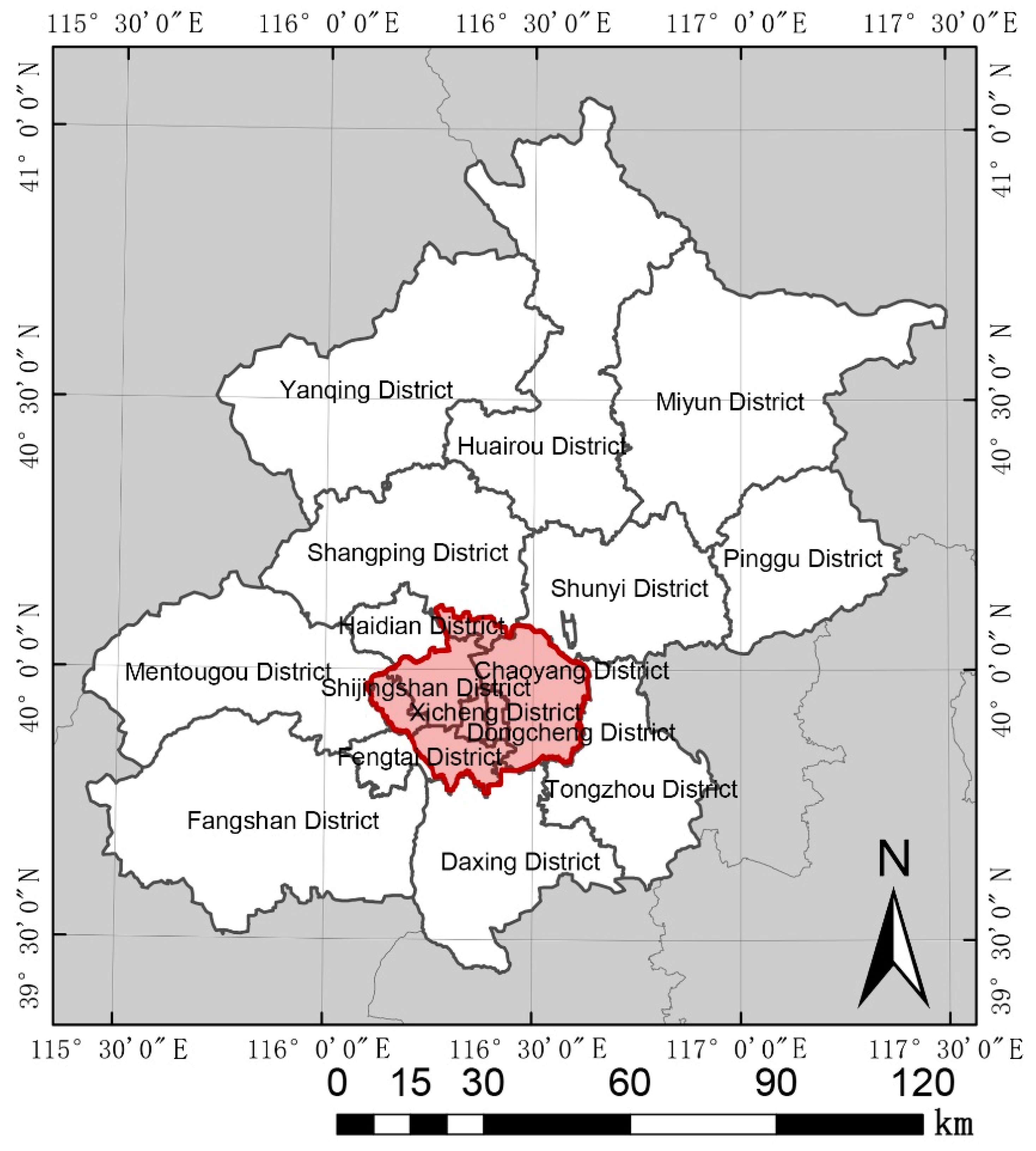
According to the Beijing City Master Plan (2004–2020), the total area of Beijing’s central district, which constitutes the study area, is 1088 km2. This area comprises Xicheng, Dongcheng, Chaoyang, and Shijingshan Districts in their entirety; most of Fengtai and Haidian Districts; Jiugong Town in Daxing District; and parts of the towns of Huilongguan and Dongxiaokou in Changping District and of Sanjiadian in Mentougou District (Figure 1).
Beijing’s Central District located in a continental climatic zone characterized by a temperate, semi-humid, and semi-arid monsoon climate. The four main seasons in this area are relatively distinct, exhibiting the following climatic characteristics: strong winds and low humidity in spring, concentrated rainfall during hot summers, and cool weather and light sunshine in autumn. The average annual temperature was 11.9 °C, with the lowest average monthly temperature of −4.3 °C recorded in January. The highest temperature was 25.9 °C. The average annual relative humidity in most parts of Beijing’s central district area is 57%, with relatively high humidity in the suburbs, ranging between 58% and 59%. During 1992–2016, Beijing’s green spaces decreased by 285.9 km2. Among these spaces, cultivated land evidenced a dramatic reduction by 246.8 km2 over this 24-year period. The extensive shrinkage of cultivated land is a central component of changes in green space that have occurred in Beijing’s central district during the study period. Woodland areas initially decreased and then increased, while grassland areas showed a steady increase. Although changes in grassland areas were relatively less than those of woodland and cultivated land, they were a key aspect of changes in green space in the central district. The increased area of grassland was attributed mainly to the construction of urban parks and golf courses, with construction and cultivated land being the primary contributors of transfer in. Dynamic changes in wetlands and water bodies in the central district were relatively insignificant, with these areas evidencing a total reduction by 23.4 km2 [50].
Within Beijing, the pace of economic development has been most rapid in the city center during the past 20 years. According to the socioeconomic data obtained for each district in Beijing’s central district in 2015, Chaoyang and Haidian Districts each have more than two million residents. Chaoyang and Haidian Districts have the highest gross region output values at over US$70.11 billion. The proportion of primary industry in the central district is almost zero. Only Chaoyang, Haidian, and Fengtai Districts have primary industry output values amounting to approximately US$15.46 million. The overall amount of secondary industry in Haidian and Chaoyang Districts is relatively high, exceeding that of Shijingshan District. However, tertiary industry currently predominates in most parts of the central district area, with Chaoyang and Haidian Districts accounting for the highest proportions of this type of industry, the values of which exceed US$61.83 billion.
2.2. Data Sources
Taking Beijing’s central district as the research object, we obtained remote sensing image data from the geospatial data cloud platform for the years 1992, 2000, 2008, and 2016. We procured digital images with a spatial resolution of 30 m from the Landsat 8 OLI_TIRS satellite data. To facilitate their interpretation, we preprocessed the remote sensing images by applying radiation calibration, atmospheric correction, and cloud removal using the ENVIMET software. Consequently, we obtained land-use data for the study area. We obtained data on the total population, greening investments, and the GDP from the Beijing Municipal Administrative Division Yearbook as well as other national repositories of economic statistics for the relevant years.
3. Construction of the SD–CA Coupling Model
3.1. The Principles Underlying the Construction of a SD–CA Coupling Model
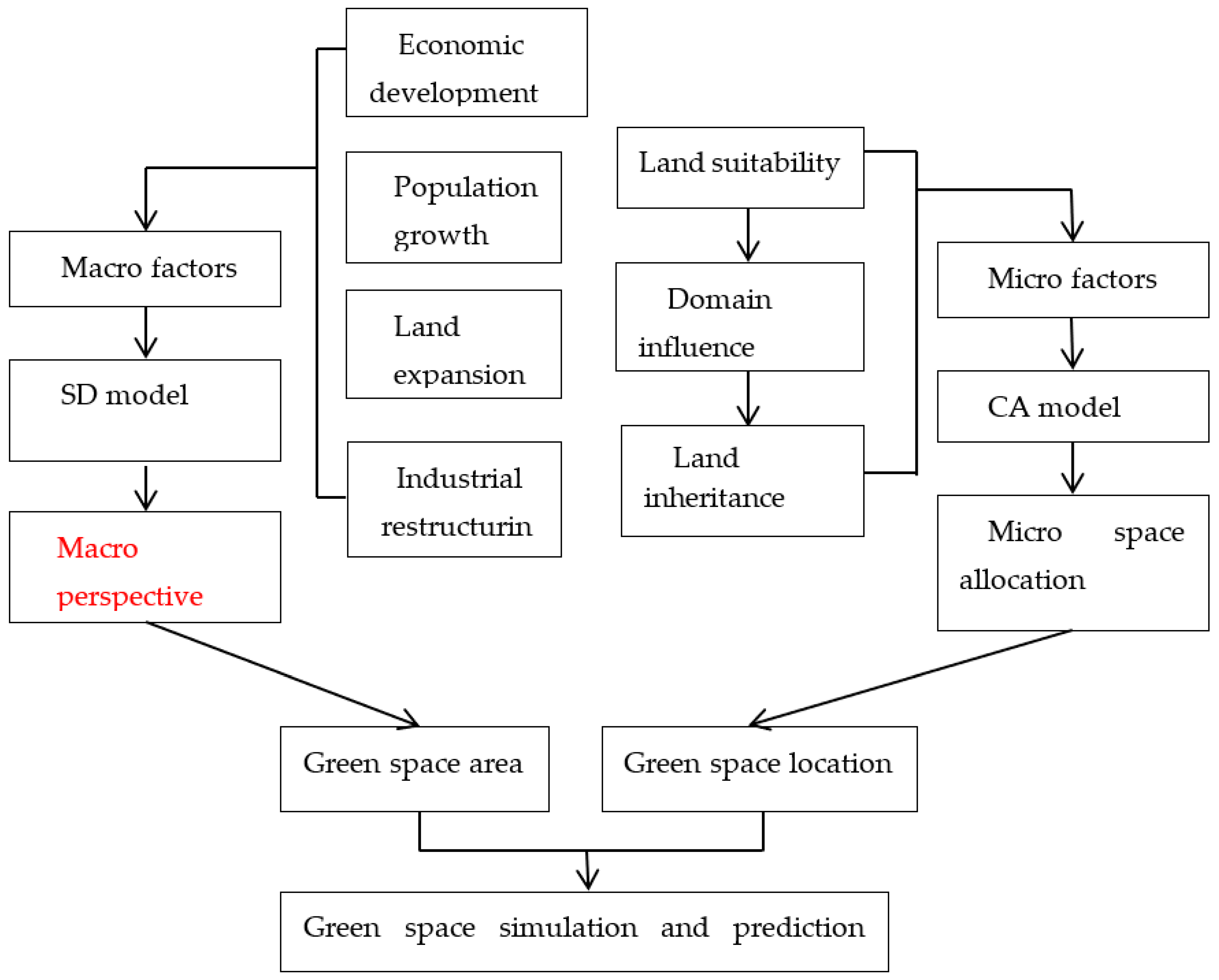
In this study, we performed coupling modeling using an SD model and a CA model (Figure 2). A differential equation was used in the SD model to conduct a top-down simulation for predicting the area of green space and determining the total area control of the simulated green space. The CA model was used to conduct bottom-up simulation and to predict the area of green space based on discrete dynamics. This model was derived from the area allocation results of coupled SD models.
We posited the following assumptions to avoid uncertain factors, thereby improving the SD–CA model’s operability. First, we assumed that socioeconomic, natural, and planning factors were the main factors driving green space evolution, with the SD model reflecting the influences of socioeconomic factors and the CA model reflecting the influences of natural and planning factors. Second, we assumed that the internal space covered within the scope of the research was a closed system. In other words, we did not consider exchanges occurring beyond the study area.
3.2. Construction of the SD Model for Conducting a Composite Simulation of Socioeconomic and Green Space Development
In this study, we predicted the green space area within Beijing’s central district, considered as a case study. The SD model incorporated macro socioeconomic factors, notably the demand for green space and the utilization of construction land [51]. It simultaneously considered green space and land that could be supplied through future transfers, thereby establishing feedback relationships among various factors within the system to achieve a balance in the supply and demand of land between the area of green space and the socioeconomic system. Thus, the SD model mainly focused on the simulation and prediction of the amount of green space driven by macro socioeconomic factors to elicit macro policy inputs for the optimization of the area of green space in the study area. Micro factors were not considered in this study. The three main components of the SD model were a causal feedback chart used to describe the causal relationship between variables, a flow chart with symbols for expressing complex concepts in the model, and differential equations comprising the bulk of the model and connecting state variables and velocity. Most of the previous studies have applied the DYNAMO equation for operation. We obtained a portrayal of the overall system, including the economic and green space subsystems that changed continuously over time, by performing a simulation using the Vensim PLE software.
3.2.1. Construction of a Causal Feedback Chart for Simulating Green Space
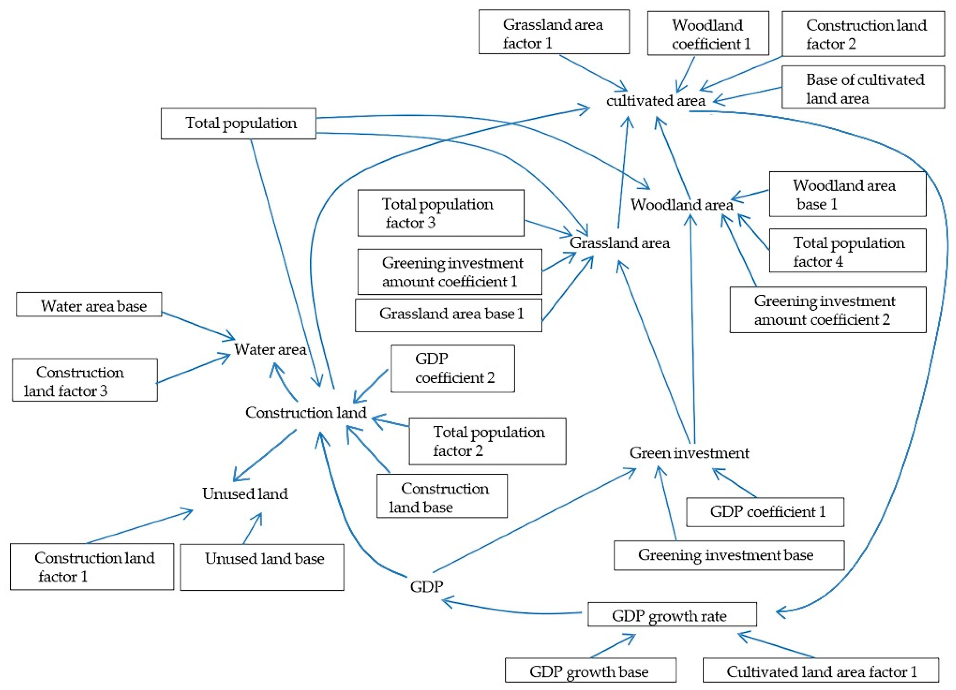
The SD model constructed for this study mainly simulated the impacts of socioeconomic factors on the area of green space in the study area. Its results were used to analyze the interaction mechanism between the socioeconomic and green space subsystems. This composite system comprised several interactive feedback loops. The system’s overall functions were constituted through interactions among these loops [52], ultimately leading to the formation of a closed green space composite system structure frame chart comprising socioeconomic and green space subsystems (Figure 3). The model’s simulation covered a period extending from 1992 to 2050. The empirical and simulation verification stages extended from 1992 to 2016, and the forecast stage extended from 2016 to 2050. The base year was 2016, and the simulation step was one year.
The green space subsystem, which is a foundational component for ensuring the ecological security of Beijing’s central district, comprised three parts: (1) four types of green space, namely cultivated land, woodland, grassland, and wetland; (2) construction land related to green space; and (3) other types of land, such as unused land. The green space subsystem not only provides recreational resources for the socioeconomic subsystem but it also provides ecological services for the urban ecosystem. Therefore, this subsystem is a core component of the composite system. There are two types of factors that influence the area of green space. The first type comprises internal factors contributing to processes of growth and decline that lead to the expansion and reduction of the area of green space, mainly as a result of the conversion of cultivated land into woodland or grassland. The second type comprises external, mainly anthropogenic factors, notably the implementation of socioeconomic policies and urban construction. Certain green spaces are occupied for anthropogenic purposes relating to production and residence, leading to a reduction in the area of green space. However, increased construction of urban parks and afforestation activities results in significant expansion of woodland and grassland areas, thereby increasing the overall area of green space.
The socioeconomic subsystem could influence and regulate the binding force of green space through an increase in the population (the number of permanent residents), socioeconomic development (the GDP), and investments in construction and supply. At the same time, the development of the green space subsystem is restricted by the occupation of areas of green space. Thus, a complex dialectical relationship exists between the socioeconomic subsystem and the green space subsystem with two key effects. First, economic growth leads to increased investments in greening and improved living standards for people that strengthen the demand for and prioritization of green space. Consequently, areas of woodland and grassland may increase. Second, GDP growth leads to improvements in public infrastructure and social facilities in cities, thereby attracting an influx of people, resulting in a dramatic increase in the pressure exerted on the ecosystems of green spaces.
We used Vensim PLE software to establish a structure flow chart of the quantitative simulation of green spaces in Beijing’s central district performed with an SD model (Figure 3) [53]. The initial values of the main state variables in the model were derived from statistical data for the period 1992–2016. The values of some of the key constants and table functions were determined with reference to the development goals for Beijing’s socioeconomic development formulated in the 12th and 13th Five-Year Plans [54,55].
3.2.2. Construction of the Equation Used for Simulating the Area of Green Space
The data simulation and prediction of the SD model was mainly determined by the equation and system operation. Three types of parameters were applied: a constant parameter whose value did not change significantly over time, a table function that solved the nonlinear simulation in the equation, and an initial value derived from statistical data. The equations were mainly used to express the mathematical relationship between an indicator and its associated indicators in the model. We applied a combination of methods to determine the equation coefficients for a scientific green space composite system. First, we statistically determined the equation coefficients of a single dependent variable based on system data obtained for the period 1992–2016. The equation forms were expressed as linear regression, logarithmic, and exponential models. R2 was generally greater than 0.6, indicating that the equation form for the explanatory variable was reasonable. The formulas of these main indicators that meet the requirements of R2 are the preliminary formulas of the model. However, statistics can only guarantee the statistical relationship between a single independent variable and the dependent variable. Usually, an indicator is not only affected by a related factor, but the change of each indicator will affect another related indicator. Therefore, when adjusting other indicators, the simulated values of indicators that have met the requirements are also changing, and some of the predicted values of indicators no longer meet the requirements of inspection accuracy. At this time, we need to adjust the model. Therefore, it was necessary to adjust the parameters manually through system debugging to ensure that the results of the simulation of the main variables of the system met the accuracy requirements. When the accuracy of the main variables all meet the requirements, the parameters and coefficients in the model together form the final formula.
3.2.3. The Model Precision Test for Simulating the Area of Green Space
To ensure the reliability and scientificity of the green space composite system model, its validity had to be tested prior to the simulation. The error rate was calculated, and the validity of the model was judged through the performance of structure, unit, and Historical data tests [56]. After conducting all of these tests, we found that the historical data as well as the simulation results met the error requirement within a 10% margin, indicating that the model was valid (Table 1).
3.2.4. Scenario Design
We applied scenario analysis to optimize the area and spatial forms of green space. The results of this analysis reflected the uncertainty of urban development and considered existing and future urban development policies as a basis for predicting the future development of the city via models [57]. We applied an SD model to simulate the green space composite system under scenarios entailing different speeds of economic development by changing the model’s parameters according to the historical data. We first selected indicators that were more sensitive to the system and had a greater impact on it and then established three scenarios (Table 2) to enable the development of an optimization plan for Beijing’s green space.
Scenario 0 was a control scenario in which the current socioeconomic development trend was maintained and used for comparison purposes in the design scenario. Scenario 1 entailed moderate socioeconomic development and population control. The population of Beijing’s central district would rise to 9.29 million in the 19th step and an average GDP would be at growth rate of 6.1% in this scenario. In Scenario 2, the pace of economic growth would continue to decline, and the population would be further reduced. The population of Beijing’s central district would reduce to 8.59 million during the 19th step and the average GDP growth rate would reduce to 4.9%.
3.3. The CA Model Used to Simulate Green Space in Beijing’s Central District
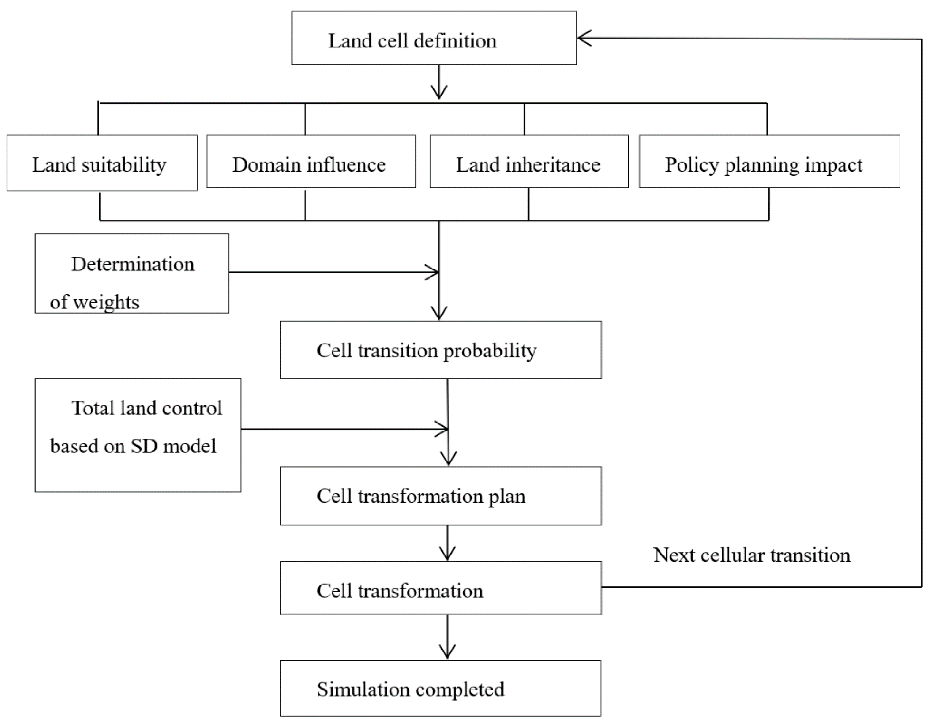
Because natural conditions could limit and affect the evolution of green space, we first deployed the powerful space simulation capabilities of the CA model, referring to existing research and the actual development of green space in Beijing’s central district. Our aim was to determine the possibility of converting land into green space, considering conversion suitability, influence of neighborhoods, and green space inheritance. The CA model has been widely used to simulate these variables, with each specific indicator obtained on the basis of a transformation rule and a thorough review of studies and data on land-use status in Beijing’s central district [58,59,60]. Considering the total forecasted results of the SD model in the scenario simulation, we simulated and predicted the spatial distribution of green space in Beijing’s central district under different economic development trends (Figure 4).
- (1)
- Cell Definition
The process of defining land cells entailed rasterizing the remote sensing data in ArcGIS, which had an accuracy of 30 m, with each cell unit having an area of 30 m × 30 m.
- (2)
- Calculation of the Probability of Cell Conversion
The probability of land cell conversion was determined by factors influencing the suitability of land conversion, the influence of neighborhoods, and land inheritance. Existing studies have generally incorporated planning-related factors into calculations of probability. Those factors comprise different variables with varying rates of contribution to land conversion. Therefore, it was necessary to determine the weight of each variable which could then be inserted through a reasonable mathematical formula to calculate the probability of each cell being converted to another cell type.
- (3)
- Determination of Conversion Rules
The conversion of land cells depended on the conversion rules. Generally, cells with a higher probability of land conversion had a higher probability of conversion. The number of cell conversions was determined by the total amount simulated in the SD model. Given this constraint on the quantity of cells, we selected the cell to be converted according to the probability of its conversion. Upon completion of each simulation, we repeated the calculation for the probability of cell conversion to guide the next cell conversion.
- (4)
- Validity Check
In the CA model, the weight setting for factors relating to the suitability of land conversion, neighborhood influence, land inheritance, and policy planning determined the probability of land cell conversion in the CA model and affected the results of the spatial simulation of land. Therefore, it was necessary to revise the simulated spatial data on the basis of historical land interpretation data and to use the Kappa coefficient as the accuracy standard for verifying the simulation results [61].
3.3.1. Simulation of the Probability of Land Conversion into Green Space
The CA model was used to determine the probability of land conversion into green space based on the suitability of the conversion, neighborhood influence, land inheritance, and the impacts of policy and planning (Table 3). In this study, we defined the probability that the land cell at position (x, y) would be converted into K-type land during period t as tPK,x,y. The suitability of K-type land for conversion was defined as tSK,x,y, the impact of the neighborhood on the conversion of a land cell into K-type land was defined as tNK,x,y, the inheritance of the land itself was defined as tIK,x,y, and the impact of planning factors on the conversion was defined as v. Thus, the probability of the land cell being transformed into K-type land was expressed as:
The specific calculation was as follows:
The suitability of land conversion was assessed in terms of the distances between the land and the road and the city center, the suitability of the land conversion in relation to the slope, and the land grade assigned to agricultural land in terms of its protection status. The following formula was used for the calculation:
where denotes the standardized value of the land suitability factor and denotes the weight of the suitability factor.
Given differences in the distances between different types of land and the road and the city center, we applied the following formula to determine the suitability of K-type land from location (x, y) to the nearest road and the city center, r, at a certain time point:
where Dr denotes the distance between the location of a land cell (x, y) and the nearest trafficable road. Because each land cell had different requirements relating to road accessibility, the correction coefficient for the accessibility of a trafficable road from a construction land unit was set to 100, and correlations for wetland and water bodies and cultivated land units were set at 50 and 10, respectively.
The suitability of different land types in relation to their slope also differed. In general, the suitability of land for cultivation had a value of 0 when the slope exceeded 25 degrees, and a value of 1 when the slope was below 25 degrees. Slope had no effect on woodland, wetland and water bodies, unused land, and grassland. The impact of slope on construction land was standardized using the following formula:
The Land and Environmental Protection Agency of the Beijing Municipal Planning Commission has explicitly advocated the protection of agricultural land in Beijing. Therefore, the probability of land conversion was determined on the basis of land grades assigned by the Land and Environmental Protection Department according to the suitability of agricultural land for cultivation.
The influence of neighborhoods (tNk,x,y) was determined based on the surrounding land types. We considered 5 × 5 neighborhood units and standardized the tNk,x,y values according to the number of K-type land units in a neighborhood.
Green space, construction land, and unused land all had varying degrees of stability relating to their inheritance status (tIk,x,y). In the CA model, the stability of the land was set as a constant value to express the land unit’s inherited status. A lower value corresponded to lower inheritance, and a greater possibility of its transfer. Fifteen experts from government agencies and universities offering urban planning and environmental science as majors were surveyed. We set the inheritance values of cultivated land, woodland, grassland, wetland and water bodies, construction land, and unused land at 0.60, 0.75, 0.40, 0.75, 1.00, and 0.00, respectively, according to the scores assigned by the experts.
The probability of land conversion into constructed land and woodland in the southeastern part of the central district increased by 0.3 and 0.1, respectively. This calculation was based on a consideration of linkages existing between land-use planning and the planning and construction of key green spaces relating to the construction of the new city of Tongzhou in Beijing.
3.3.2. Conversion Rules for Green Space Simulation
We performed space allocation simulations of Beijing’s green space, construction land, and unused land based on the various land area requirements determined using the SD model.
Rule 1: The CA model was used to simulate spatial conversions between green space and construction and unused land. The following conversions were considered based on the current status of land use in the central district area and a literature review.
Cultivated land could be either protected—and was therefore not transferable—or transferred. Cultivated land that was transferable could be converted into construction land (for urban expansion and construction), woodland (plain afforestation or conversion of cropland into forests and parks), grassland (park and golf course construction), and wetland and water bodies (park construction and the restoration of water systems).
Woodland could be protected—and therefore not transferable—or transferred. Woodland that was not protected could be converted into construction land (for urban expansion and construction), grassland (for park and golf course construction), or wetland and water bodies (for park construction and the restoration of water systems).
Grassland could be converted into grassland, construction land (for urban expansion and construction), woodland (for park construction), or wetland and water bodies (for park construction and the restoration of water systems).
Wetland and water bodies could be converted into wetland and water bodies, construction land (for urban expansion and construction), or woodland (park construction).
Construction land could be converted into construction land, woodland (park construction), grassland (park and golf course construction), or wetland and water bodies (park construction and the restoration of water bodies).
Unused land could be converted into unused land, construction land, woodland (park construction) and grassland (park and golf course construction).
Rule 2: The total amount of land determined in the SD model simulation would be allocated in the following order: construction land, cultivated land, woodland, grassland, wetland and water bodies, and unused land. After allocating the total amount of land of the first type, allocation of the second type of land would be carried out. Moreover, after completing the conversion of one type of land, it would not be converted again during the simulation period.
Rule 3: A land cell at (x, y) location was defined as tPK,x,y relating to land selection according to the probability of its conversion into K-type land in period t. Cell units with a higher probability of being converted into K-type land than other land types in Beijing’s central district would be selected first. These cell units would be selected in descending order of the probability of their conversion until the total demand for K-type land was satisfied.
3.3.3. Verification and Revision of Green Space Simulations
The weight setting of the influence of neighborhood size and inheritance based on different factors would affect calculations of the probability of converting different green spaces and hence the simulation results. Therefore, it was essential to revise the spatial model using relevant data. We conducted simulations based on land interpretation data for Beijing’s central district in 1992 and 2000 and revised the simulated data for 2008 and 2016. The Kappa coefficients for the simulation results in 2008 and 2016 were 0.7813 and 0.8076, respectively, which met accuracy requirements.
4. Results and Analysis
4.1. Composite SD Model Simulation Results for Socioeconomic and Green Space Development
After conducting modeling using the Vemsim PLE software, we performed the simulation using interpreted remote sensing data for the period 1992–2016. Maintaining the current socioeconomic development status, we simulated land-use data for 2017–2050 at one-year intervals, considering 2016 as the base year. The simulation and prediction results are shown in Table 4.
The results shown in Table 4 indicate that if socioeconomic development in Beijing’s central district continues at its current pace, the current change trend for green space and constructed land would also continue over the next 30 years. Notably, the area of cultivated land would decrease significantly before 2030. Moreover, under the pressure of economic development and population growth, cultivated land would basically disappear by 2036. From the overall perspective of land conversion, most of the converted cultivated land would be occupied by construction land, leading to a continuous increase in the area of construction land that would peak at 90,801.42 ha by 2036. The areas of woodland and grassland would increase slightly, with the area of woodland increasing from 14,337.74 ha to 15, 342.79 ha, and the area of grassland increasing from 2199.071 ha to 2785.597 ha in 2050. However, wetland would completely disappear by 2037, while unused land would disappear by 2027. In sum, if the current socioeconomic development trend in Beijing’s central district continues, the land development trend would entail conversion of the remaining areas of cultivated land into construction land for urban expansion and the steady expansion of areas of woodland and grassland.
4.2. Results of the CA Model Simulation of Green Space
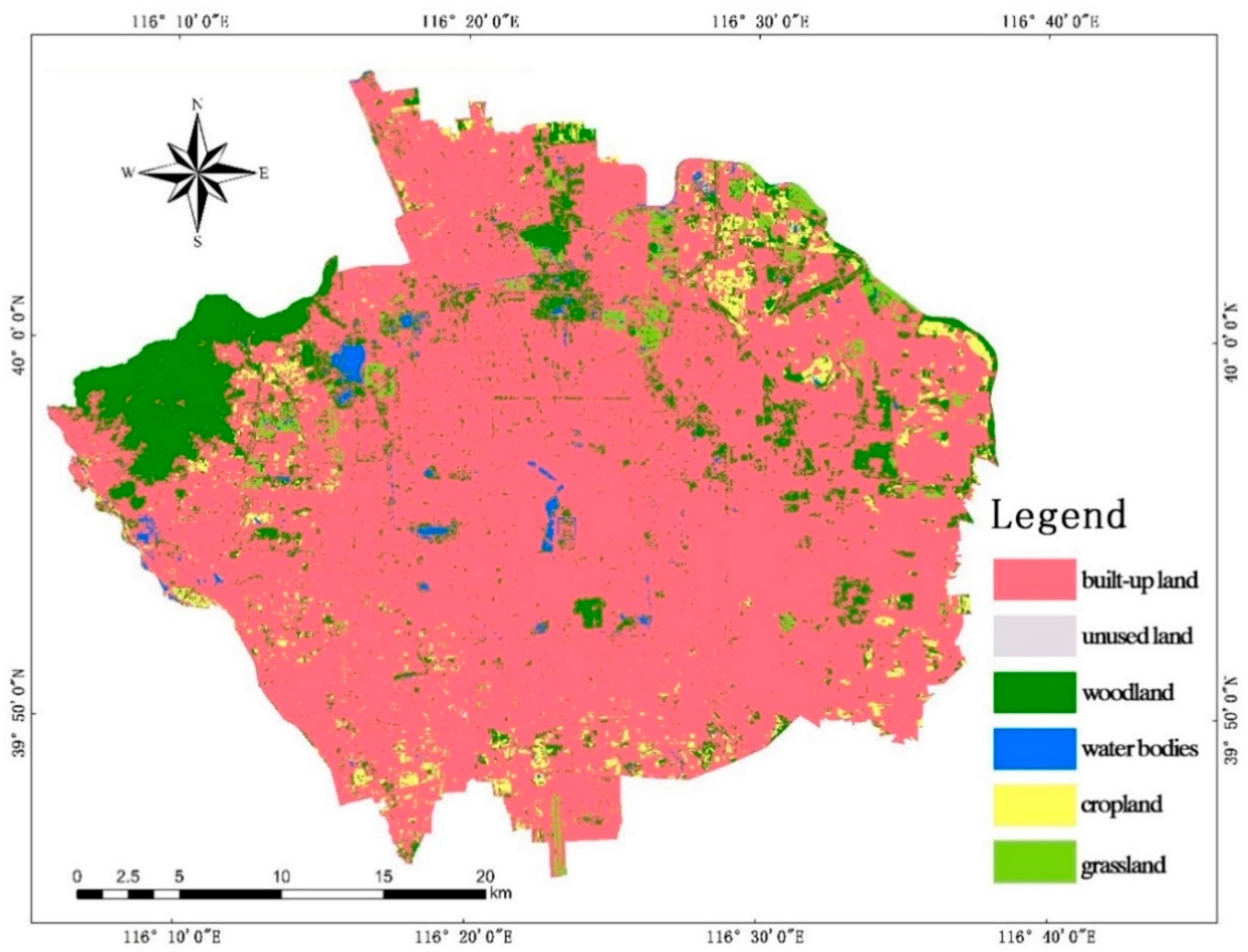
Applying the interpreted remote sensing data for Beijing’s central district in 2016 as the benchmark data, we simulated and predicted future year-end areas of green space, construction land, and unused land in Beijing’s central district according to the current socioeconomic development trend. This scenario was deemed Scenario 0 in which the specific area was determined by the simulation value. The simulation and prediction results are shown in Figure 5.
If the current socioeconomic development trend continues, extensive tracts of cultivated land along the border of Chaoyang District, in the southern part of the central district (where cultivated land is fragmented), and in the western suburbs of Xishan Piedmont would be transformed into construction land. Woodland would increase to some extent in the western suburbs and at the northeastern boundaries of the area adjacent to the main road. Most of the water bodies in the central district would be used to meet construction needs. Overall, green space would continue to be transformed into built-up land as a result of urban construction, especially in Beijing’s central district.
4.3. Prediction and Optimization of Green Space under Different Scenarios
We used an SD model to simulate and predict areas of land under three scenarios. We also used a CA model to allocate areas of green space under different speeds of economic development, enabling us to predict areas of green space in 2035 (Figure 6 and Figure 7). Moreover, we compared the landscape pattern of green spaces in Beijing’s central district under three scenarios at the end of the simulation period. We did so by calculating the patch areas, percentages of patch areas, average patch area, number of patches, patch densities, the maximum patch index, the edge density, the landscape shape index, the connectivity index, and Shannon diversity index of green space (Table 5).
The results showed evident differences in the predicted green spaces in Beijing’s central district under different scenarios in 2035. Specifically, in Scenario 0 in which the current socioeconomic development trend continued, the shape of the green space in Beijing’s central district, considered in terms of the landscape pattern index, would become less complex and diverse by 2035. The area of green space would be dramatically reduced as a result of its conversion for urban construction, and the amount and percentage of patch areas would be considerably lower compared with those in other scenarios. Of all the scenarios, Scenario 0 was associated with the lowest Shannon diversity index value, indicating that the integrity and diversity of green spaces was also threatened by urban construction.
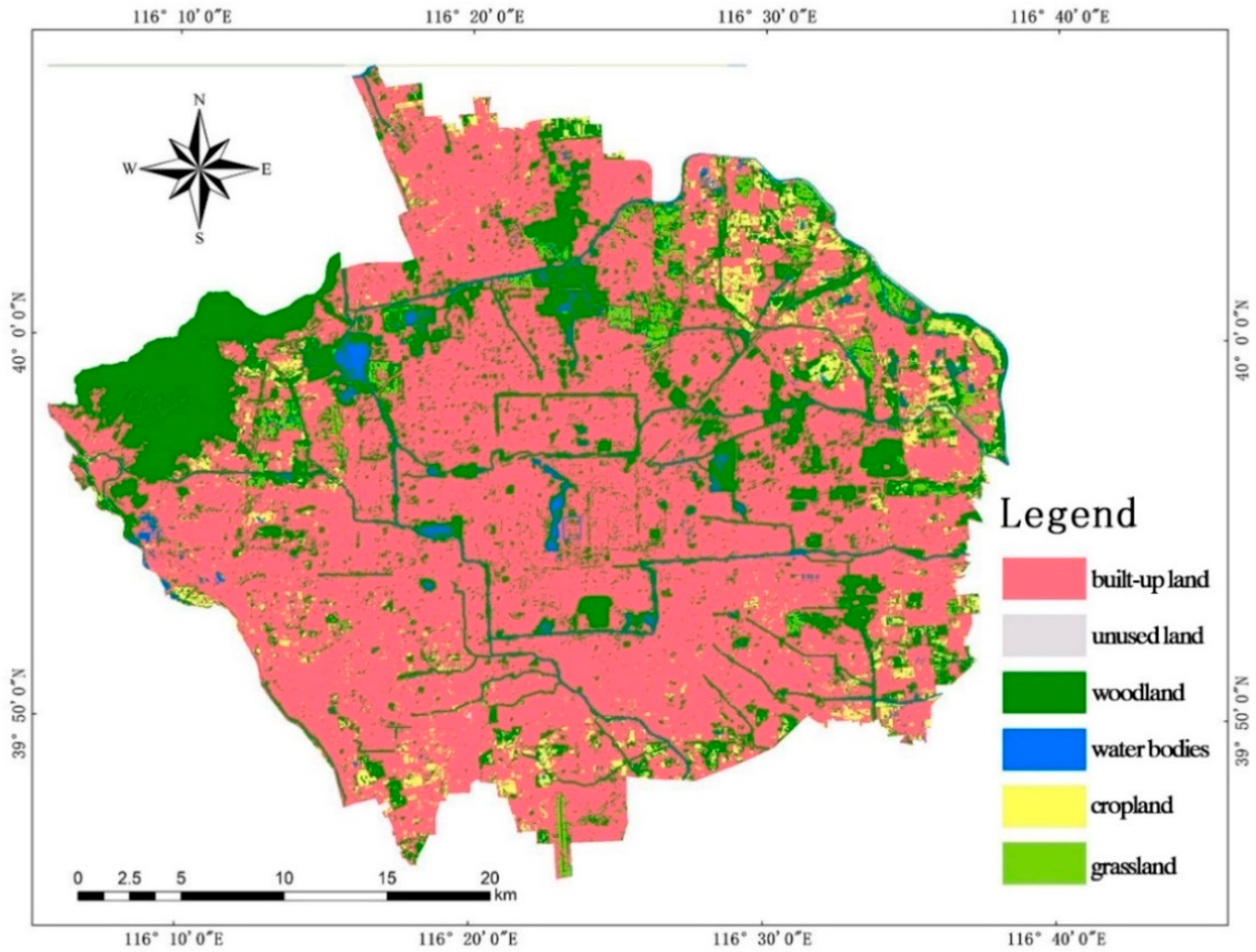
In Scenario 1, appropriate slowing down of economic development to a moderate pace combined with the control of population growth would result in slight changes in the areas of the various types of land by 2035 as a result of the interplay of ecological conservation of green spaces and economic development. From a spatial perspective, cultivated land in the southeastern part of the central district would fragment and disappear. Taking into account the construction of the new city of Tongzhou, woodland areas in the southeastern part of the central district would increase slightly in this scenario. The extent of the decrease in the area of cultivated land would be less compared with the decrease of this land under Scenario 0. Moreover, the patch density, landscape shape index, and edge density values of green space would be higher compared with those for Scenario 0 mainly because of the fragmentation of cultivated land in the southeastern part of the central district.
In Scenario 2 in which the pace of economic development would continue to slow down and population growth would be further controlled relative to Scenario 1, the goal of ecological conservation could be achieved through natural restoration as well as efforts to protect and take care of green spaces. By 2035, the most apparent change in the various land types would be a decrease in the area of construction land, while areas of woodland, grassland, and wetland and water bodies could increase. In Scenario 2, the percentage of patches of green space could increase significantly with corresponding decreases in the densities and edge densities of these patches, indicating a distinct decrease in the fragmentation of green spaces. Further, the connectivity and diversity indexes of green spaces would clearly improve, indicating significant optimization of green spaces in Beijing’s central district according to an ideal pattern. In sum, economic development and ecological conservation would be effectively combined and balanced from a longer-term perspective. Thus, the maintenance of the quantity and quality of urban green spaces requires attention, with prioritization of the overall, long-term, and dynamic development of green spaces. Moreover, ecological conservation, restoration, and construction must be conducted simultaneously, while balancing ecological and economic benefits.
5. Discussion
5.1. Result Analysis
Combining the SD and CA models, we developed a new model for predicting green space that incorporated and integrated socioeconomic factors. The model was simultaneously used to conduct a spatial analysis of the prediction results, enabling the simulation of green space planning scenarios and the determination of reasonable green space and socioeconomic development indicators. Unlike the models applied in previous studies for evaluating water, energy, and food security [62,63,64], this spatiotemporal simulation model can provide direct inputs and guidelines for planning. Our analysis of historical data for the period 1992–2016 revealed that green space development would be restricted if the current pace of Beijing’s socioeconomic development is maintained. This finding is consistent with the results of ecological and socioeconomic forecasting trends reported in earlier studies [50,65]. The relationship between socioeconomic development and green space is evidently complicated. On the one hand, socioeconomic development will lead to increased green investments and promote green space development, including the construction of urban parks. On the other hand, increasing areas of green space will be occupied as a result of socioeconomic development. Therefore, under the current scenario of socioeconomic development, green space development will be inhibited [66,67,68]. Accordingly, we designed two other scenarios based on existing policies.
In scenario 2, which was the first of these two simulated scenarios, a reduction in the population to 8.59 million by 2035, with an average GDP growth rate of 4.9% was associated with a substantial increase in the proportion of Beijing’s green space up to 40%. This ratio is optimal and leads to comprehensive benefits derived from green space, including ecological safety and recreational facilities. However, a considerable gap exists between this ideal scenario and the current situation relating to Beijing’s socioeconomic development because planning entails not only questions of quantity but also those relating to space. The problem of rationally identifying new green spaces in the current cultural context is a challenging one. Our simulation, generated through the CA model, indicated that by 2035, the population would decrease to 9.29 million, with an average GDP growth rate of 6.1% relative to scenario 0, potentially leading to the occupation of a large amount of the historical space in scenario 1 by green space. From the perspective of socioeconomic requirements, it would be relatively easy to increase the proportion of green space appropriately at this time. At the same time, the results of the CA model showed that most of the newly added green spaces would be relatively reasonable.
5.2. A Comparative Analysis of the Development of Green Space in International Metropolises
Beijing, London, Paris, and New York are typical international metropolises that have all faced thorny urban issues in the course of their development. However, all of these international cities adopted timely and effective response strategies that offer insights for Beijing. For example, New York City embarked on the “PlaNYC: A Greener, Greater New York” initiative to address climate change and preserve biodiversity. Detailed planning strategies for land, water, and transportation management were formulated, with the aim of developing New York into a “greener and better” international metropolis. Consequently, positive results were achieved relating to urban ecological issues such as biodiversity conservation. The initiative also entailed a specific focus on green open spaces that were considered separately within a special land project in which linear connections among urban green spaces were emphasized.
To control smog in London, a large circular green space was constructed around the city, and the urban transportation system was organically integrated with green open spaces through a greenway system and green wedge to create a complete urban ecological network. The linear “green chain” was constructed to create an efficient urban ventilation system. The wind flow from the Thames blowing in from the eastern part of the city cleared air pollutants, while the wind from the west brought fresh air into the city, effectively reducing its smog.
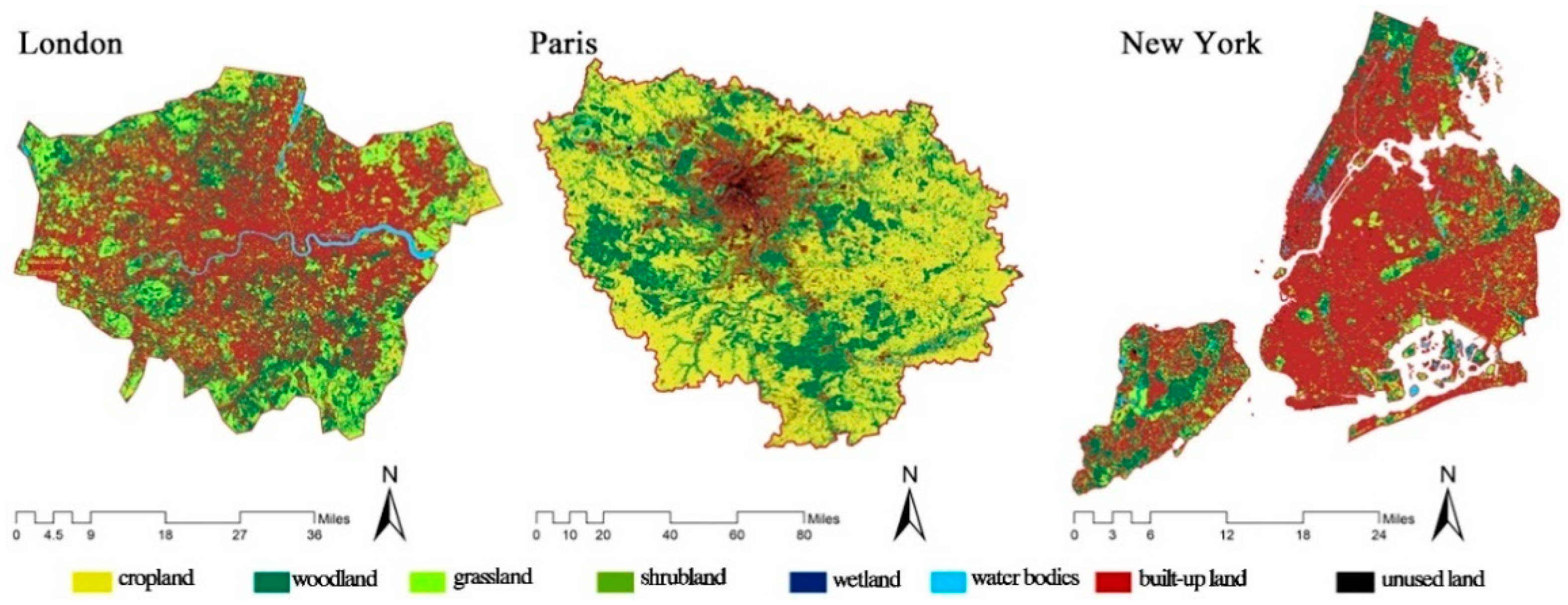
We calculated the landscape pattern index values of the main green spaces in the three international metropolises in 2016 and compared their patterns of green space with that of Beijing’s central district in 2035 (Figure 8 and Table 6). Specifically, we analyzed the characteristics of the green space distribution in these international metropolises from the perspective of their green space patterns.
Although the green space coverage of most cities was less than 60%, some landscape pattern indexes, such as the fragmentation index, had a significant relationship with the atmospheric dust retention effect of green spaces and the improvement of the atmospheric environment. A comparison of the degree of fragmentation of green spaces in Beijing under Scenario 2 and in London revealed that the patch density of the green space pattern in Beijing would be less than that of London’s built-up area in 2035. This result indicates that the degree of fragmentation of green spaces in Beijing would be slightly lower than that of London’s built-up area. Considered only from the perspective of fragmentation and the mitigation of air pollution, the mitigation capacity of the green space predicted under Scenario 2 in Beijing’s central district would be slightly higher than that of London’s built-up area. A comparison of the green space connectivity of Beijing and New York revealed that the value of the connectivity index of Beijing’s green space pattern would be slightly smaller than that of New York’s built-up area in 2035. Considered only from the perspective of green space connectivity and biodiversity, biodiversity protection within green spaces in Beijing’s central district would be weaker than that in New York.
5.3. Policy Recommendations and Limitations of the Study
Because of the high density of built-up areas in Beijing’s central district, it would not be possible to rely completely on the demolition of constructions on existing land to increase the area of green space in Scenarios 1 or 2. In the old city, the development of small and micro green spaces, making full use of unused waste land, and the renovation of parking lots to increase green space could be considered as possible options. In the vicinity of the Fourth Ring Road where urban construction is relatively complete, linear green spaces could be fully availed of, for example, through the construction of green roads and the linking of existing green spaces. In addition, the construction of the first green barrier in Beijing should be thoroughly explored, and a search should be conducted for more flexible spaces in this area for carrying out large-scale planning of green spaces.
This study also had some limitations. First of all, the integration of Beijing-Tianjin-Hebei allows for their interlinked socioeconomic development. However, we did not consider the development of linkages between Beijing’s central district and surrounding areas, which is an important direction for future system optimization. Second, this study was based on the prevailing land-use classification system and did not include a more detailed classification of green space, which could have affected the accuracy of the results. Last, spatially-oriented research is evidently an important direction for future research, which should entail a comprehensive consideration of the impacts of cultural spaces and functions on the conversion of green spaces and other types of land use.
6. Conclusions
In this study, we applied an SD model to simulate the area of green space in Beijing’s central district during the period 2016–2050. The results of the simulation revealed that if the current pace of socioeconomic development in the central district continued, the current change trends for green space and construction land would also continue over the next 30 years. The overall area of green space would continue to decrease, with the area of cultivated land decreasing significantly before 2030 and basically disappearing in 2036. The area of construction land would continue to increase, reaching its peak value by 2036. Moreover, there would be a small increase in woodland and grassland areas. Wetland and water bodies and unused land would continue to decrease, eventually disappearing in 2037 and 2027, respectively.
Moderate socioeconomic development and the control of population growth would be required to achieve Scenario 1. In this scenario, when the population of Beijing’s central district reached 9.29 million by the 19th step, and an average GDP growth rate of 6.1% was maintained, the area of green space would be 20,454.07 ha. Under Scenario 2, the pace of economic growth would continue to slow down, and the population would be further reduced. By the 19th step, a reduction in the population of Beijing’s central district to 8.59 million and a reduction in the average GDP growth rate to 4.9% would correspond to an area of 40,678.02 ha occupied by green space.
Our CA model results also revealed evident differences in the green spaces of Beijing’s central district in 2035 under different scenarios. In Scenario 0 in which the current socioeconomic development trend continued, an extensive area of cultivated land would be occupied by construction land by 2035, and most of the water bodies in the central part of the central district would be drained to provide construction land. Moreover, the shapes of the green spaces would also become more complex, and their diversity would decline further. Economic development at a moderate pace and controlled population growth in Scenario 1 would be associated with fragmentation and the disappearance of cultivated land in the southeastern part of the central district. However, there would be a slight increase in forested land in the southeastern part of the city. In a context of low-speed economic development and further population shrinkage in Scenario 2, the most obvious change in the various land types would be a decrease in the area of construction land and expanded areas of woodland, grassland, and wetland and water bodies by 2035. The fragmentation of green spaces would decrease significantly, with a corresponding significant increase in green space connectivity and the diversity index. Thus, under Scenario 2, the green spaces within Beijing’s central district would be significantly optimized.
Author Contributions
Conceptualization, F.L. and S.L.; methodology, F.L.; software, M.S.; validation, F.L., S.L. and J.D.; formal analysis, F.L.; investigation, J.D.; resources, Q.S.; data curation, F.L.; writing—original draft preparation, F.L.; writing—review and editing, R.W.; visualization, J.D. and Q.S.; supervision, S.L.; project administration, F.L.; funding acquisition, S.L. All authors have read and agreed to the published version of the manuscript.
Funding
This work was supported by the National Natural Science Foundation of China (Grant No. 51908036, 41871175), Beijing Natural Science Foundation (Grant NO. 8194071, 9184035); Youth Foundation for Humanities and Social Sciences Research of the Ministry of Education (NO. 19YJC760042); a grant from Beijing Key Laboratory of Spatial Development for Capital Region (CLAB202006); the Fundamental Research Funds for the Central Universities (NO. BLX201808,2018RW01). Research and Development Plan of Beijing Municipal Science and Technology Commission (Grant No. D17110900710000), the Social Science Foundation of Beijing (grant no. 16SRB011), and Beijing Forestry University Outstanding Young Talent Cultivation Project (grant no. 2019JQ03011).
Data Availability Statement
The data presented in this study are available on request from the first author.
Conflicts of Interest
The authors declare no conflict of interest.
References
- Wolch, J.R.; Byrne, J.; Newell, J.P. Urban green space, public health, and environmental justice: The challenge of making cities ‘just green enough’. Landsc. Urban Plan. 2014, 125, 234–244. [Google Scholar] [CrossRef] [Green Version]
- Chen, T.; Lang, W.; Li, X. Exploring the Impact of Urban Green Space on Residents’ Health in Guangzhou, China. J. Urban Plan. Dev. 2020, 146, 05019022. [Google Scholar] [CrossRef]
- Wu, J.; He, Q.; Chen, Y.; Lin, J.; Wang, S. Dismantling the fence for social justice? Evidence based on the inequity of urban green space accessibility in the central urban area of Beijing. Environ. Plan. B Urban Anal. City Sci. 2020, 47, 626–644. [Google Scholar] [CrossRef]
- Sathyakumar, V.; Ramsankaran, R.; Bardhan, R. Geospatial approach for assessing spatiotemporal dynamics of urban green space distribution among neighbourhoods: A demonstration in Mumbai. Urban For. Urban Green. 2020, 48, 126585. [Google Scholar] [CrossRef]
- Jim, C.Y.; Chen, S.S. Comprehensive greenspace planning based on landscape ecology principles in compact Nanjing city, China. Landsc. Urban Plan. 2003, 65, 95–116. [Google Scholar] [CrossRef]
- Chen, H.; Ganesan, S.; Jia, B. Environmental challenges of post-reform housing development in Beijing. Habitat Int. 2005, 29, 571–589. [Google Scholar] [CrossRef]
- Li, F.; Wang, R.; Paulussen, J.; Liu, X. Comprehensive concept planning of urban greening based on ecological principles: A case study in Beijing, China. Landsc. Urban Plan. 2005, 72, 325–336. [Google Scholar] [CrossRef]
- Koprowska, K.; Łaszkiewicz, E.; Kronenberg, J. Is urban sprawl linked to green space availability? Ecol. Indic. 2020, 108, 105723. [Google Scholar] [CrossRef]
- De Sousa, C.A. Turning brownfields into green space in the City of Toronto. Landsc. Urban Plan. 2003, 62, 181–198. [Google Scholar] [CrossRef]
- Portillo-Quintero, C.A.; Sanchez, A.M.; Valbuena, C.A.; Gonzalez, Y.Y.; Larreal, J.T. Forest cover and deforestation patterns in the Northern Andes (Lake Maracaibo Basin): A synoptic assessment using MODIS and Landsat imagery. Appl. Geogr. 2012, 35, 152–163. [Google Scholar] [CrossRef]
- Gobster, P.H.; Westphal, L.M. The human dimensions of urban greenways: Planning for recreation and related experienc-es. Landsc. Urban Plan. 2004, 68, 147–165. [Google Scholar] [CrossRef]
- Weber, C.; Puissant, A. Urbanization pressure and modeling of urban growth: Example of the Tunis Metropolitan Area. Remote Sens. Environ. 2003, 86, 341–352. [Google Scholar] [CrossRef]
- Ma, J.; Haarhoff, E. The GIS-based research of measurement on accessibility of green infrastructure-a case study in Auck-land. In MIT CUPUM Conference Proceeding, Proceedings of the 14th International Conference on Computers in Urban Planning and Urban Management, Adelaide, Australia, 7–10 July 2015; MIT Press: Cambridge, MA, USA, 2015. [Google Scholar]
- Lu, S.; Guan, X.; He, C.; Zhang, J. Spatio-temporal patterns and policy implications of urban land expansion in metropolitan ar-eas: A case study of Wuhan urban agglomeration, central China. Sustainability 2014, 6, 4723–4748. [Google Scholar] [CrossRef] [Green Version]
- Pan, D.; Domon, G.; De Blois, S.; Bouchard, A. Temporal (1958–1993) and spatial patterns of land use changes in Haut-Saint-Laurent (Quebec, Canada) and their relation to landscape physical attributes. Landsc. Ecol. 1999, 14, 35–52. [Google Scholar] [CrossRef]
- Wu, J.; Hobbs, R. Key issues and research priorities in landscape ecology: An idiosyncratic synthesis. Landsc. Ecol. 2002, 17, 355–365. [Google Scholar] [CrossRef]
- Yokohari, M.; Bolthouse, J. Planning for the slow lane: The need to restore working greenspaces in maturing contexts. Landsc. Urban Plan. 2011, 100, 421–424. [Google Scholar] [CrossRef]
- Aydin, M.B.S.; Çukur, D. Maintaining the carbon–oxygen balance in residential areas: A method proposal for land use plan-ning. Urban For. Urban Green. 2012, 11, 87–94. [Google Scholar] [CrossRef]
- Lee, A.C.K.; Maheswaran, R. The health benefits of urban green spaces: A review of the evidence. J. Public Health 2010, 33, 212–222. [Google Scholar] [CrossRef]
- Du, M.; Zhang, X. Urban greening: A new paradox of economic or social sustainability? Land Use Policy 2020, 92, 104487. [Google Scholar] [CrossRef]
- Jo, H.K. Impacts of urban greenspace on offsetting carbon emissions for middle Korea. J. Environ. Manag. 2002, 64, 115–126. [Google Scholar] [CrossRef]
- De Ridder, K.; Adamec, V.; Bañuelos, A.; Bruse, M.; Bürger, M.; Damsgaard, O.; Dufek, J.; Hirsch, J.; Lefebre, F.; Pérez-Lacorzana, J.M.; et al. An integrated methodology to assess the benefits of urban green space. Sci. Total Environ. 2004, 334, 489–497. [Google Scholar] [CrossRef] [PubMed]
- Xiao, X.D.; Dong, L.; Yan, H.; Yang, N.; Xiong, Y. The influence of the spatial characteristics of urban green space on the urban heat island ef-fect in Suzhou Industrial Park. Sustain. Cities Soc. 2018, 40, 428–439. [Google Scholar] [CrossRef]
- Yamamoto, Y. Measures to Mitigate Urban Heat Islands; NISTEP Science & Technology Foresight Center: Tokyo, Japan, 2006.
- Conine, A.; Xiang, W.-N.; Young, J.; Whitley, D. Planning for multi-purpose greenways in Concord, North Carolina. Landsc. Urban Plan. 2004, 68, 271–287. [Google Scholar] [CrossRef]
- Kong, F.; Yin, H.; Nakagoshi, N.; Zong, Y. Urban green space network development for biodiversity conservation: Identification based on graph theory and gravity modeling. Landsc. Urban Plan. 2010, 95, 16–27. [Google Scholar] [CrossRef]
- Gairola, S.; Noresah, M.S. Emerging trend of urban green space research and the implications for safeguarding biodiversi-ty: A viewpoint. Nat. Sci. 2010, 8, 43–49. [Google Scholar]
- Aida, N.; Sasidhran, S.; Kamarudin, N.; Aziz, N.; Puan, C.L.; Azhar, B. Woody trees, green space and park size improve avian biodiversity in urban landscapes of Peninsular Malaysia. Ecol. Indic. 2016, 69, 176–183. [Google Scholar] [CrossRef]
- Zhang, H.; Chen, B.; Sun, Z.; Bao, Z. Landscape perception and recreation needs in urban green space in Fuyang, Hangzhou, China. Urban For. Urban Green. 2013, 12, 44–52. [Google Scholar] [CrossRef]
- Lu, S.; Zhou, M.; Guan, X.; Tao, L. An integrated GIS-based interval-probabilistic programming model for land-use planning management under uncertainty—A case study at Suzhou, China. Environ. Sci. Pollut. Res. 2014, 22, 4281–4296. [Google Scholar] [CrossRef]
- Dang, A.N.; Kawasaki, A. A Review of Methodological Integration in Land-Use Change Models. Int. J. Agric. Environ. Inf. Syst. 2016, 7, 1–25. [Google Scholar] [CrossRef]
- López, E.; Bocco, G.; Mendoza, M.; Duhau, E. Predicting land-cover and land-use change in the urban fringe: A case in Morelia city, Mexico. Landsc. Urban Plan. 2001, 55, 271–285. [Google Scholar] [CrossRef]
- Cheng, J.; Masser, I. Urban growth pattern modeling: A case study of Wuhan city, PR China. Landsc. Urban Plan. 2003, 62, 199–217. [Google Scholar] [CrossRef]
- Kong, F.; Nakagoshi, N. Spatial-temporal gradient analysis of urban green spaces in Jinan, China. Landsc. Urban Plan. 2006, 78, 147–164. [Google Scholar] [CrossRef]
- Kong, F.; Yin, H.; James, P.; Hutyra, L.R.; He, H.S. Effects of spatial pattern of greenspace on urban cooling in a large metropolitan area of eastern China. Landsc. Urban Plan. 2014, 128, 35–47. [Google Scholar] [CrossRef]
- Batty, M.; Couclelis, H.; Eichen, M. Urban Systems as Cellular Automata. Environ. Plan. B Plan. Des. 1997, 24, 159–164. [Google Scholar] [CrossRef]
- Costanza, R.; Rüth, M. Using Dynamic Modeling to Scope Environmental Problems and Build Consensus. Environ. Manag. 1998, 22, 183–195. [Google Scholar] [CrossRef] [PubMed]
- Shen, Q.; Chen, Q.; Tang, B.-S.; Yeung, S.; Hu, Y.; Cheung, G. A system dynamics model for the sustainable land use planning and development. Habitat Int. 2009, 33, 15–25. [Google Scholar] [CrossRef]
- White, R.; Engelen, G. Cellular automata as the basis of integrated dynamic regional modelling. Environ. Plan. B Plan. Des. 1997, 24, 235–246. [Google Scholar] [CrossRef]
- De Almeida, C.M.; Batty, M.; Monteiro, A.M.V.; Câmara, G.; Soares-Filho, B.S.; Cerqueira, G.C.; Pennachin, C.L. Stochastic cellular automata modeling of urban land use dynamics: Empirical development and estimation. Comput. Environ. Urban Syst. 2003, 27, 481–509. [Google Scholar] [CrossRef]
- Li, X.; Yeh, A.G.O. Modelling sustainable urban development by the integration of constrained cellular automata and GIS. Int. J. Geogr. Inf. Sci. 2000, 14, 131–152. [Google Scholar] [CrossRef]
- Ward, D.; Murray, A.; Phinn, S. A stochastically constrained cellular model of urban growth. Comput. Environ. Urban Syst. 2000, 24, 539–558. [Google Scholar] [CrossRef]
- Barredo, J.I.; Kasanko, M.; McCormick, N.; LaValle, C. Modelling dynamic spatial processes: Simulation of urban future scenarios through cellular automata. Landsc. Urban Plan. 2003, 64, 145–160. [Google Scholar] [CrossRef]
- Caruso, G.; Peeters, D.; Cavailhès, J.; Rounsevell, M. Space–time patterns of urban sprawl, a 1D cellular automata and microeconomic approach. Environ. Plan. B Plan. Des. 2009, 36, 968–988. [Google Scholar] [CrossRef] [Green Version]
- Sterman, J.D. System Dynamics Modeling: Tools for Learning in a Complex World. Calif. Manag. Rev. 2001, 43, 8–25. [Google Scholar] [CrossRef]
- Li, F.; Lu, S.; Sun, Y.; Li, X.; Xi, B.-Y.; Liu, W. Integrated Evaluation and Scenario Simulation for Forest Ecological Security of Beijing Based on System Dynamics Model. Sustainability 2015, 7, 13631–13659. [Google Scholar] [CrossRef] [Green Version]
- Wang, H.; Li, M.; Hu, N.; Gao, Y. Utilization effectiveness of marine functional zones using system dynamics for China: Mod-eling and assessment. J. Coast. Conserv. 2014, 18, 609–616. [Google Scholar] [CrossRef]
- Guo, H.; Liu, L.; Huang, G.; Fuller, G.; Zou, R.; Yin, Y. A system dynamics approach for regional environmental planning and management: A study for the Lake Erhai Basin. J. Environ. Manag. 2001, 61, 93–111. [Google Scholar] [CrossRef] [Green Version]
- Zhang, H. A simulation of the dynamics of soil erosion in the loess hills of Shanxi and Shaanxi provinces. Chin. Sci. Bull. 1997, 42, 743–746. [Google Scholar]
- Li, F.; Zheng, W.; Wang, Y.; Liang, J.; Xie, S.; Guo, S.; Li, X.; Yu, C. Urban Green Space Fragmentation and Urbanization: A Spatiotemporal Perspective. Forests 2019, 10, 333. [Google Scholar] [CrossRef] [Green Version]
- Jin, X.; Xu, X.; Xiang, X.; Bai, Q.; Zhou, Y. System-dynamic analysis on socio-economic impacts of land consolidation in China. Habitat Int. 2016, 56, 166–175. [Google Scholar] [CrossRef]
- Kombe, W.J. Land use dynamics in peri-urban areas and their implications on the urban growth and form: The case of Dar es Salaam, Tanzania. Habitat Int. 2005, 29, 113–135. [Google Scholar] [CrossRef]
- de SI Gonçalves, J.C.; Giorgetti, M.F. Mathematical model for the simulation of water quality in rivers using the VENSIM PLE® software. J. Urban Environ. Eng. 2013, 7, 48–63. [Google Scholar] [CrossRef] [Green Version]
- Beijing Municipal Development and Reform Commission. Outline of the Twelfth Five-Year Plan for Beijing’s National Economic and Social Development; China Population Press: Beijing, China, 2011. [Google Scholar]
- Outline of the Thirteenth Five-Year Plan for Bei-jing’s Na-tional Economic and Social Development. Bull. Standing Comm. Beijing Munic. Peoples Congr. 2016, 001, 20–81. (In Chinese)
- Barlas, Y. Formal aspects of model validity and validation in system dynamics. Syst. Dyn. Rev. J. Syst. Dyn. Soc. 1996, 12, 183–210. [Google Scholar] [CrossRef]
- Landis, J.; Zhang, M. The second generation of the California urban futures model. Part 2: Specification and calibration re-sults of the land-use change submodel. Environ. Plan. B Plan. Des. 1998, 25, 795–824. [Google Scholar] [CrossRef]
- Li, Y.C.; He, C.Y. Scenario simulation and forecast of land use/cover in northern China. Chin. Sci. Bull. 2008, 53, 1401–1412. [Google Scholar] [CrossRef] [Green Version]
- He, C.; Okada, N.; Zhang, Q.; Shi, P.; Zhang, J. Modeling urban expansion scenarios by coupling cellular automata model and system dynamic model in Beijing, China. Appl. Geogr. 2006, 26, 323–345. [Google Scholar] [CrossRef]
- Long, Y.; Shen, Z. An urban model using complex constrained cellular automata: Long-term urban form prediction for Beijing. Int. J. Soc. Syst. Sci. 2011, 3, 159–173. [Google Scholar] [CrossRef]
- Zheng, F.; Hu, Y. Assessing temporal-spatial land use simulation effects with CLUE-S and Markov-CA models in Beijing. Environ. Sci. Pollut. Res. 2018, 25, 32231–32245. [Google Scholar] [CrossRef]
- Sahin, O.; Stewart, R.A.; Porter, M.G. Water security through scarcity pricing and reverse osmosis: A system dynamics approach. J. Clean. Prod. 2015, 88, 160–171. [Google Scholar] [CrossRef] [Green Version]
- Prambudia, Y.; Nakano, M. Integrated Simulation Model for Energy Security Evaluation. Energies 2012, 5, 5086–5110. [Google Scholar] [CrossRef]
- Xu, J.; Ding, Y. Research on early warning of food security using a system dynamics model: Evidence from Jiangsu province in China. J. Food Sci. 2015, 80, R1–R9. [Google Scholar] [CrossRef] [PubMed]
- Li, F.; Sun, Y.; Li, X.; Hao, X.; Li, W.; Qian, Y.; Liu, H.; Sun, H. Research on the Sustainable Development of Green-Space in Beijing Using the Dynamic Systems Model. Sustainability 2016, 8, 965. [Google Scholar] [CrossRef] [Green Version]
- Qian, Y.; Zhou, W.; Li, W.; Han, L. Understanding the dynamic of greenspace in the urbanized area of Beijing based on high resolution satellite images. Urban For. Urban Green. 2015, 14, 39–47. [Google Scholar] [CrossRef]
- Jim, C. Green-space preservation and allocation for sustainable greening of compact cities. Cities 2004, 21, 311–320. [Google Scholar] [CrossRef]
- Barbosa, O.; Tratalos, J.A.; Armsworth, P.R.; Davies, R.G.; Fuller, R.A.; Johnson, P.; Gaston, K.J. Who benefits from access to green space? A case study from Sheffield, UK. Landsc. Urban Plan. 2007, 83, 187–195. [Google Scholar] [CrossRef]
Figure 1.
Location of Beijing’s Central District.

Figure 2.
Framework of the SD–CA Coupling Model for Predicting Green Spaces in Beijing’s Central District.
Figure 2.
Framework of the SD–CA Coupling Model for Predicting Green Spaces in Beijing’s Central District.

Figure 3.
The SD Model’s Causal Feedback Chart Depicting the Composite System of Green Space in Beijing’s Central District. Note: Construction land was delineated into the following urban and rural land-use categories: industrial, mining, and residential land.
Figure 3.
The SD Model’s Causal Feedback Chart Depicting the Composite System of Green Space in Beijing’s Central District. Note: Construction land was delineated into the following urban and rural land-use categories: industrial, mining, and residential land.

Figure 4.
The Framework Developed for the CA Modeling Process.

Figure 5.
Results of the CA Model Simulation of Green Spaces in Beijing’s Central District in 2035.

Figure 6.
Results of the CA Model Simulation of Green Spaces in Beijing’s Central District in 2035 (Scenario 1).
Figure 6.
Results of the CA Model Simulation of Green Spaces in Beijing’s Central District in 2035 (Scenario 1).

Figure 7.
Results of the CA Model Simulation of Green Spaces in Beijing’s Central District in 2035 (Scenario 2).
Figure 7.
Results of the CA Model Simulation of Green Spaces in Beijing’s Central District in 2035 (Scenario 2).

Figure 8.
The Distribution of Green Spaces in Three International Metropolises in 2016.


Table 1.
Error Testing of the Green Space Composite System.
| Time(Year) | GSA (ha) | CLA (ha) | CL (ha) | WDA (ha) | WDWA (ha) | ULA (ha) | |
|---|---|---|---|---|---|---|---|
| 1992 | ALV | 1837 | 32,254 | 54,539 | 16,419 | 3865 | 16 |
| SIV | 1825.57 | 25,531.4 | 59,132.9 | 11,846.3 | 3589.65 | 14.4498 | |
| ER | 0.0062 | 0.2084 | 0.0842 | 0.2785 | 0.0712 | 0.0968 | |
| 2000 | ALV | 1919 | 21,171 | 70,499 | 12,402 | 2929 | 10 |
| SIV | 1912.44 | 20,112.4 | 66,971.8 | 12,410.2 | 2899.83 | 11.7846 | |
| ER | 0.0034 | 0.05 | 0.0500 | 0.0006 | 0.0099 | 0.1784 | |
| 2008 | ALV | 2094 | 10,452 | 80,492 | 14,561 | 1322 | 8 |
| SIV | 2104.68 | 10,613.6 | 80,131.2 | 13,582.8 | 1454.86 | 7.31038 | |
| ER | 0.0051 | 0.0154 | 0.0044 | 0.0671 | 0.1005 | 0.0862 | |
| 2016 | ALV | 2248 | 6251 | 84,811 | 14,176 | 1438 | 5 |
| SIV | 2232.58 | 5490.92 | 87,141.7 | 14,247 | 1124.88 | 4.92684 | |
| ER | 0.0068 | 0.1215 | 0.0274 | 0.0050 | 0.2177 | 0.0146 |
Notes: GSA = grassland area, GLA = cultivated area, CL = construction land, WDA = woodland area, WDWA = wetland and water area, ULA = unused land area, ALV = actual values, SIV = simulated values of the composite system of green space based on the SD model, ER = error rates.
Table 2.
Different Scenarios of the Green Space Composite System Developed for Beijing’s Central District.
Table 2.
Different Scenarios of the Green Space Composite System Developed for Beijing’s Central District.
| Situation Name | Scenario Description | Involving Indicators Description |
|---|---|---|
| Scenario 0 | Socioeconomic development keeps the status. | Socioeconomic development keeps the status. |
| Scenario 1 | Appropriately reduce the speed of economic development, and control population growth. | The population will decrease to 9.29 million by 2035, with an average GDP growth rate of 6.1%. |
| Scenario 2 | Based on Scenario 1, continue to reduce the speed of economic development, and further control population growth. | Population will be reduced to 8.59 million by 2035, with an average GDP growth rate of 4.9%. |
Table 3.
Mode of Variable Acquisition in the CA Model of Green Space Simulations in Beijing’s Central District.
Table 3.
Mode of Variable Acquisition in the CA Model of Green Space Simulations in Beijing’s Central District.
| Classification | Variable | Method of Obtaining | Range of Raw Data Values |
|---|---|---|---|
| Land conversion suitability | Distance from road | GIS measures distance and normalizes according to formula | 0–1 |
| Distance from city center (Tiananmen) | GIS measures distance and normalizes according to formula | 0–1 | |
| Slope | DEM data and construction land are standardized according to formulas, others see text description | 0–1 | |
| Land grade for agricultural land suitability (cultivated land protection) | Land and Environmental Protection Agency of Beijing Municipal Planning Commission, 1988 | ||
| Neighborhood influence | Units of cultivated land in the neighborhood | 5 × 5 neighborhood unit | 0–24, Need to be standardized |
| Units of woodland in the neighborhood | 5 × 5 neighborhood unit | 0–24, Need to be standardized | |
| Number of grassland units in the neighborhood | 5 × 5 neighborhood unit | 0–24, Need to be standardized | |
| Number of wetland and waters units in the neighborhood | 5 × 5 neighborhood unit | 0–24, Need to be standardized | |
| Number of units for construction land in the neighborhood | 5 × 5 neighborhood unit | 0–24, Need to be standardized | |
| Number of units in unused neighborhood | 5 × 5 neighborhood unit | 0–24, Need to be standardized | |
| Land inheritance | Land use status type | Land use status map and results of dynamic simulation | 0.65, 0.9, 0.8, 0.7, 1, 0.65 |
| Policy planning factors | The location of the land cellular | 0.3, 0.1 |
Note: Raw data values for neighborhood influence ranged from 0 to 24. Given that this range differed from those for other indicators, it was standardized to 0–1.
Table 4.
Results of the Simulation of Green Space in Beijing’s Central District.
| Time (Year) | GSA (ha) | CLA (ha) | CL (ha) | WDA (ha) | WDWA (ha) | ULA (ha) |
|---|---|---|---|---|---|---|
| 2016 | 2199.071 | 6730.502 | 84,411.91 | 14,337.74 | 1247.463 | 3.313752 |
| 2027 | 2426.956 | 939.582 | 90,272.44 | 14,973.07 | 317.9496 | 0 |
| 2030 | 2698.368 | 189.582 | 90,713.94 | 15,255.53 | 72.58259 | 0 |
| 2036 | 2785.402 | 0 | 90,801.42 | 15,342.59 | 0.582586 | 0 |
| 2037 | 2785.597 | 0 | 90,801.61 | 15,342.79 | 0 | 0 |
| 2050 | 2785.597 | 0 | 90,801.61 | 15,342.79 | 0 | 0 |
Note: GSA = grassland area, GLA = cultivated area, CL = construction land, WDA = woodland area, WDWA = wetland and water area, and ULA = unused land area.
Table 5.
Predicted Landscape Metrics Relating to Green Spaces in Beijing’s Central District in 2035.
Table 5.
Predicted Landscape Metrics Relating to Green Spaces in Beijing’s Central District in 2035.
| CA | PLAND | NP | PD | LPI | ED | LSI | AREA_MN | COHESION | SHDI | |
|---|---|---|---|---|---|---|---|---|---|---|
| Scenario 0 | 18,022.88 | 16.57 | 7557 | 6.95 | 4.33 | 39.84 | 81.98 | 2.38 | 97.74 | 0.44 |
| Scenario 1 | 21,561.04 | 19.82 | 7687 | 7.06 | 4.41 | 46.63 | 87.94 | 2.80 | 97.86 | 0.49 |
| Scenario 2 | 48,079.28 | 40.42 | 7312 | 5.25 | 4.92 | 32.26 | 76.45 | 2.98 | 98.25 | 0.52 |
Note: CA = patch area, PLAND = percentage of patch area, NP = patch number, PD = patch density, LPI = largest patch index, ED = edge density, LSI = landscape shape index, AREA_MN = average patch area, COHESION = connectivity index, and SHDI = Shannon diversity index.
Table 6.
A Comparison of Green Space Patterns in Beijing’s Central District with Landscape Patterns in Three International Metropolises in 2035.
Table 6.
A Comparison of Green Space Patterns in Beijing’s Central District with Landscape Patterns in Three International Metropolises in 2035.
| PD | COHESION | SHDI | |
|---|---|---|---|
| Beijing’s central district Scenario 0 | 6.9501 | 97.7469 | 0.4491 |
| Beijing’s central district Scenario 1 | 7.0697 | 97.8603 | 0.4985 |
| Beijing’s central district Scenario 2 | 5.2561 | 98.2567 | 0.5278 |
| London built-up area | 7.3694 | 99.3663 | 1.2014 |
| Paris built-up area | 6.6252 | 99.0174 | 1.4180 |
| New York built-up area | 7.7823 | 98.3931 | 1.0013 |
Note: PD = patch density, COHESION = connectivity index, and SHDI = Shannon diversity index.
Publisher’s Note: MDPI stays neutral with regard to jurisdictional claims in published maps and institutional affiliations. |
© 2021 by the authors. Licensee MDPI, Basel, Switzerland. This article is an open access article distributed under the terms and conditions of the Creative Commons Attribution (CC BY) license (http://creativecommons.org/licenses/by/4.0/).
Share and Cite
MDPI and ACS Style
Li, F.; Wang, R.; Lu, S.; Shao, M.; Ding, J.; Sun, Q. Spatiotemporal Simulation of Green Space by Considering Socioeconomic Impacts Based on A SD-CA Model. Forests 2021, 12, 202. https://0-doi-org.brum.beds.ac.uk/10.3390/f12020202
AMA Style
Li F, Wang R, Lu S, Shao M, Ding J, Sun Q. Spatiotemporal Simulation of Green Space by Considering Socioeconomic Impacts Based on A SD-CA Model. Forests. 2021; 12(2):202. https://0-doi-org.brum.beds.ac.uk/10.3390/f12020202
Chicago/Turabian StyleLi, Fangzheng, Rongfang Wang, Shasha Lu, Ming Shao, Jingyi Ding, and Qianxiang Sun. 2021. "Spatiotemporal Simulation of Green Space by Considering Socioeconomic Impacts Based on A SD-CA Model" Forests 12, no. 2: 202. https://0-doi-org.brum.beds.ac.uk/10.3390/f12020202
Note that from the first issue of 2016, this journal uses article numbers instead of page numbers. See further details here.