
Mapping Floods in Lowland Forest Using Sentinel-1 and Sentinel-2 Data and an Object-Based Approach


1
Chair of Photogrammetry and Remote Sensing, Faculty of Geodesy, University of Zagreb, Kačićeva 26, 10000 Zagreb, Croatia
2
Production and Development Department, Croatian Forests Ltd., Ivana Meštrovića 28, 48000 Koprivnica, Croatia
*
Author to whom correspondence should be addressed.
Forests 2021, 12(5), 553; https://0-doi-org.brum.beds.ac.uk/10.3390/f12050553
Submission received: 16 March 2021
/
Revised: 21 April 2021
/
Accepted: 26 April 2021
/
Published: 28 April 2021
(This article belongs to the Special Issue Remote Sensing Applications in Forests Inventory and Management)
Abstract
:The impact of floods on forests is immediate, so it is necessary to quickly define the boundaries of flooded areas. Determining the extent of flooding in situ has shortcomings due to the possible limited spatial and temporal resolutions of data and the cost of data collection. Therefore, this research focused on flood mapping using geospatial data and remote sensing. The research area is located in the central part of the Republic of Croatia, an environmentally diverse area of lowland forests of the Sava River and its tributaries. Flood mapping was performed by merging Sentinel-1 (S1) and Sentinel-2 (S2) mission data and applying object-based image analysis (OBIA). For this purpose, synthetic aperture radar (SAR) data (GRD processing level) were primarily used during the flood period due to the possibility of all-day imaging in all weather conditions and flood detection under the density of canopy. The pre-flood S2 imagery, a summer acquisition, was used as a source of additional spectral data. Geographical information system (GIS) layers—a multisource forest inventory, habitat map, and flood hazard map—were used as additional sources of information in assessing the accuracy of and interpreting the obtained results. The spectral signature, geometric and textural features, and vegetation indices were applied in the OBIA process. The result of the work was a developed methodological framework with a high accuracy and speed of production. The overall accuracy of the classification is 94.94%. Based on the conducted research, the usefulness of the C band of the S1 in flood mapping in lowland forests in the leaf-off season was determined. The paper presents previous research and describes the SAR parameters and characteristics of floodplain forest with a significant impact on the accuracy of classification.
1. Introduction
Floods are associated with high rainfall intensities and occur when recipients cannot receive all the water, causing them to spill over into the surrounding areas [1]. Flooded areas are land susceptible to being inundated by water from any source, which usually presents as low, frequently flooded habitats along the coast on river islands and reefs, usually in the river’s immediate vicinity depending on the micro-relief and in remote areas of the river valley [2]. About 9% of the land area of the Republic of Croatia (approximately 500,000 ha) can be described as a frequently flooded area, which means that there occurs at least one flooding event in a period of three to five years, and part of that area can be considered as wetland habitats [2]. Floodplain forests and rivers are an indivisible whole. In the floodplain, the appearance of forest stands (morphology) and the spatial distribution of wood biomass (structure) are particularly affected by the water regime and edaphic features. Any change in the water regime affects forest stands, especially their origin and dynamics. This impact can be direct (frequency, height and duration of floodwaters, and the occurrence of floodwater freezing) and indirect (spatial and temporal dynamics of soil moisture, groundwater, and precipitation) [3].
For the analysis and management of floods and the assessment of damages, it is necessary to determine the maximum extent of floods [4], so it is extremely important to define the boundaries of flooded areas as quickly as possible [5]. The boundaries of flooded areas can be collected by in situ [6] or remote sensing data [7,8,9,10]. The extent of flooding determined in situ has shortcomings due to the possible limited spatial and temporal resolution data at a significant cost [11].
Remote sensing data such as aerial [12] and satellite imagery [13] as well as other geospatial data [14] are useful in mapping and monitoring wetlands. Aerial imagery is traditionally used [4], with the beginning of this century representing the starting point of the effective application of multispectral and synthetic aperture radar satellite (SAR) imagery in the mapping and monitoring of these habitats [15,16]. Despite the above, the robustness of most of today’s radar satellite sensors is often an obstacle for detailed and accurate mapping of the wetlands; namely, the image resolution is too low [17]. On the other hand, high spatial resolution optical sensors allow more accurate determination of floodplain boundaries [4]. However, the data quality depends on weather conditions [5]; in the case of cloud or fog, the optical sensor cannot provide quality information [11,18]. Additional problems are present in areas overgrown with dense forests covering water surfaces and preventing the penetration of radiation through dense forest canopies [19] and in the case where water surfaces are covered with floating and other vegetation [12].
It is difficult to detect inundation (flooding) under tree canopies (e.g., dense and closed forests) with the optical spectrum, except in cases of an open and incomplete canopy [20]. Satellite overflights often do not coincide with the moment of reaching the extreme value of the analyzed phenomenon when it comes to archival images [5], while for accurate flood detection and associated dynamics, they require a short revisit time (temporal resolution) [17]. Therefore, the absence of additional corrections may result in an underestimated or overestimated size of the flooded area [5,21].
SARs are active sensors that operate in the microwave part of the electromagnetic spectrum. They are considered active because they have an energy source (impulses of a certain wavelength and polarization) that emits and receives backscattering (reflection) of the measured surface [22,23]. SAR remote sensing depends on the availability of SAR scenes and the purpose of a particular mission. Most satellite SAR missions are operational in the X (2.5–3.75 cm), C (3.75–7.5 cm), or L band (15–30 cm) [20,23]. The attractiveness of the SAR is due to the operational advantage of conducting all-day (7/24) imaging [24]. Compared to most other sensors, these advantages allow imaging (monitoring and mapping) of the Earth regardless of weather conditions (clouds, fog, rain, and other weather disasters) and lighting [23,25]. Therefore, they are becoming an increasingly important source of environmental information [26]. Moreover, SAR impulses after emits have an interaction with the observed surface area and then receive backscattering signals that create imagery totally different to optical sensors. Based on that, SAR imagery allows the acquisition of additional data (new information) regarding the environment [27]. Objects in SAR scenes may differ if the associated backscatter components are different and if the spatial resolution is sufficient to distinguish the objects [28].
The strength (intensity) of the feedback signal is expected to increase during the presence of water under the vegetation canopy due to double or multiple interactions between the water surface and the vertical vegetation structure [20]. During the first studies of the application of SAR to the observation of objects on Earth, it was previously observed that floods under the forest canopy could be detected due to increased feedback (scattering) caused by the interaction of water and stems [29]. Therefore, in wet habitats in woody vegetation, the presence of water under the canopy increases the feedback signal, while it is weakened in grassy (herbaceous) vegetation [30]. As floods are often associated with heavy rain (and other atmospheric disturbances), which makes optical satellite data inaccessible [31], SAR sensors have proven to be more suitable than optical instruments in flood detection under forest canopies [7,15,20,29,32].
Due to the ecological complexity of wetland habitats, it is considered useful to use different sensors (imaging in a wide range of the electromagnetic spectrum) to collect diverse data in order to increase the accuracy of classification (mapping) [20]. In this sense, multispectral and SAR data have advantages and disadvantages [16]. Optical data provide spectral characteristics of the measured area and objects, while SAR data provide information on the structure of vegetation, soil moisture, and flooded vegetation [33]. Since each sensor measures different characteristics, it is expected that the integration of optical and SAR data will increase classification accuracy in wetland mapping [16,20].
Thus, SAR systems provide the possibility of continuous data collection, regardless of weather conditions and lighting, which allows the rapid mapping of changes in the environment [31]. In the literature [34,35], the process of creating a map in a short period is colloquially called “fast mapping”. According to Copernicus Emergency Management Services [36], the process is deemed fast when a map is created in less than 12 h from data acquisition to the production of the final product (so-called delineation and grading products). Therefore, the main purpose of this paper is to develop and apply a methodological framework of satisfactory accuracy and acceptable cost and time (speed) for monitoring and mapping of floods in lowland forests using Sentinel-1 (S1) and Sentinel-2 (S2) images.
In the realization of the goal, by integrating S1 and S2 data, we attempted to use the advantages (data and information) of each sensor and increase the accuracy of classification by fusion, a synergy effect. On the other hand, it is necessary to accept, as stated in the review paper [37], that vegetation in the low/moderate stage of growth is mainly considered separately in relation to high vegetation (e.g., forest) due to the different effects of vegetation structure and density on SAR signal intensities. Furthermore, the interpretation of the feedback SAR signal from different objects in the conditions of the existence or absence of flooding continues to be a research challenge [7,32]. Therefore, this paper selects and analyzes the environmentally diverse research area (grasslands, bushwood, agricultural land, and forests of different types and stages) to assess the applicability of Sentinel-1 (S1) and Sentinel-2 (S2) imagery in flood mapping in more complex (heterogeneous) environmental conditions.
2. Materials and Methods
2.1. SAR Parameters and Forest Characteristics for Floodplain Mapping
The application of SAR in the mapping and monitoring of flooded vegetation is based on a proper understanding of the interaction of impulse and vegetative backscattering under certain conditions [32]. Namely, the same observation object in different geographical locations, different periods, or different climate and seasonal variations does not have the same image. Moreover, the signal’s backscattering and the measuring quality of the imaged object also change with the change in the SAR sensor parameters: polarization, wavelength, and local angle of incidence [26,38]. Furthermore, assuming the constancy of SAR sensor parameters, which is true for SAR systems with a repeated trajectory (orbit) [19], the intensity of reflected SAR signals is a function of heterogeneity (roughness) of the measured surface and conductivity and dielectricity of the Earth’s surface [32]. Thus, in the case of SAR sensor constancy, changes in the imagery are conditioned only by variations of the observed object and not by other factors [19]. Water has one of the highest values of the dielectric constant among all-natural substances, and the reflection of soil and plants is largely dependent on water content [26]. In the case of forests, this means that the SAR reflection primarily depends on the forest structure (canopy, density, leaves, trunks, etc.) and associated geometric features and secondarily on the dielectric properties of the imaged forest [39].
The characteristics of the observed object and sensor parameters, namely, the wavelengths, frequency, polarization of the transmitted and received signal, incidence angle, and direction of observation, determine the strength of the feedback signal (scattering) [38]; therefore, they must be taken into account when interpreting and analyzing the SAR data [7,19]. Researchers [7,30,40,41,42,43] have described the interaction of SAR impulses with forest and forestland. In this regard, the authors of [41] describe the interaction of the forest and the L band, which consists of the following: (i) diffuse scattering from the forest floor, (ii) volume scattering from the forest canopy, (iii) scattering from the canopy signal to the soil and trunks, and (iv) specular reflection from the forest soil and trunks (Figure 1).
The authors of [4,7,13,32,37,38,44] indicate that composite feedback SAR signal (Figure 1) increases in the flooded forest compared to non-flood conditions. The basic explanation of the increased (amplified) feedback signal of flooded forests is the double-bounce reflection (rectangular or full). It is a complex phenomenon that depends on microwaves’ ability to transmit energy through a forest canopy. In the case of penetration through the forest canopy to the trunks, this reflection additionally depends on the existence of vertical reflection, respectively, the interaction between the surface (in this case, water) and the stand layer of trunks (dihedral angle), which scatter energy in the direction of the SAR antenna [43].
It should be borne in mind that there are transitions (forest edges–semi-forested areas) between low and sparse woody vegetation to high forest, and that the forest is a heterogeneous system in which there are groups of trees or stands of lower height and low density, sporadically or over a larger area. In these relationships, increased rectangular reflection is not expected because the trees are low, the associated trunks are short and small in diameter, and the dominance of double-bounce reflection is absent [42,45]. The described conditions present a disturbance in the detection of flooding in the forest by the SAR because the feedback signal’s strength is in the transition between open flood (submerged area) with weak feedback and flooding under the forest canopy with strong feedback.
It is important to note that this phenomenon predominates in longer wavelength sensors (L band) with HH polarization; for this reason, the combination of these two parameters is considered most expedient in forest flood detection [37,42,46]. In shorter wavelength sensors—the C and X bands—volume scattering of signals from the tree crown significantly attenuates or completely prevents penetration through the forest canopy, thus eliminating vertical reflection [41]. In general, longer wavelengths have a greater capacity for the SAR signal to penetrate vegetation (forest) canopy.
In particular, some authors are of the opinion that microwaves of shorter wavelengths (C and X bands) are not useful in mapping or monitoring forest floods [17,30,42,46,47]. Namely, the main disadvantage of the C band in flood mapping under the forest canopy (Figure 2) is the attenuation of the signal from the canopy (leaves and needles) of trees or the insufficient wavelength [20,29]. On the other hand, studies have been published confirming the acceptability of C and X bands in flood detection under a forest canopy. In these papers, the authors describe the forest’s structural characteristics and seasonal predispositions in which the double-bounce phenomenon can be realized. In this sense, the author of [43] affirmatively expresses the application of C bands in flood detection in forests and states that it is necessary to determine the stand structure and conditions under which floods can be detected using SAR C band VV sensors. In former research [43], the author emphasizes that elements that attenuate the microwave signal as it passes through the forest canopy should be considered as well as those elements under the canopy that amplify rectangular backscattering. Using the ERS1 C band VV sensor, it was determined that a high stand basal area, greater heights from the bottom of the canopy, and openness of the layer under the canopy increase the backscattering in the flooded forests of the investigated area. Interestingly, the author did not determine a significant impact of the forest canopy (measured: leaf area index, crown closure, and canopy depth), which the author himself considers an unexpected result [43].
In general, the result is considered more reliable in sparse vegetation [48] or leaf-off conditions [20,30,43,49,50,51]. Exceptionally affirmative results of the use of X band in the detection of flooded forest have been presented in the research of [29,45] using TerraSAR-X and Cosmo Sky-Med data.
Polarization represents the orientation of the electromagnetic field vector with respect to propagating the SAR signal. Polarization in conventional (single-polarized) SAR systems is horizontal (H) and/or vertical (V) and the signal can be transmitted and received as co-polarization (HH or VV) and cross-polarization (HV or VH). Dual SAR systems transmit either the H- or V-polarized signal and receive both feedback signals (HH and VV, HH and HV, and VV and HV). SAR systems with a full polarimetric system transmit H- and V-polarized signals alternately and receive both orthogonal polarizations (HH, VV, and HV and VH) [26,28].
In the mapping of flooded forests using conventional (single-polarized) SAR systems, reference is made to using HH polarizations versus VV polarization [32,43,48]. Namely, the rectangular reflection’s contribution (appearance) (double bounce) in the trunk–surface interaction is weaker in VV polarization. Dual SAR systems are useful for generating data and information from two polarizations ratios [37]. In general, the use of more advanced SAR systems and different polarization combinations opens up opportunities for obtaining new data (Table 1). Therefore, in the process of flood monitoring and mapping, the choice of the appropriate polarization is of paramount importance.
The incidence angle is defined as the angle between the direction perpendicular to the Earth’s surface and the incident SAR impulse [26]. Depending on the satellite sensor, the angles of incidence range between 10° and 65°; the larger angles of incidence are marked as shallow, and the smaller angles are steep [37]. A steeper angle of incidence is considered more suitable for flood mapping in forests due to the canopy’s shorter path. Namely, in this case, the transmission of the forest canopy is increased, and, as a result, a more frequent interaction between the trunks and the surface is enabled (the appearance of rectangular reflection). By contrast, a shallow incidence angle increases interaction with the forest canopy and consequently increases volume reflection [48,50]. Thus, the impact of the incidence angle on SAR data quality is significant [38].
In addition, the strength of SAR backscattering is conditioned by the state of the environment and flooded vegetation (community, biomass, phenology, soil moisture, water depth, etc.) [37]. Furthermore, the SAR is sensitive to soil moisture and water in vegetation, open water, and water under the forest canopy. As such, the increase in moisture in the soil and vegetation increases the backscattering. In addition to the moisture element, the horizontal and vertical stand structure significantly influences the backscattering [19]. The capacity of all SAR systems (including the L and P bands) to penetrate a forest canopy may be reduced or completely absent depending on tree density, the density of canopy, and tree height. Namely, SAR backscattering is correlated with the biomass as the wavelength increases, and the biomass is also correlated with the saturation point [52], where it is no longer possible to detect flooding under the forest canopy. In this case, the volume reflection completely covers (superimposes) the double-bounce reflection, i.e., the interaction between the trunks and the water surface. Consequently, the saturation point depends on the described SAR parameters and forest structure. In this regard, the phenology of vegetation and the presence of leaves (leaf-on/leaf-off conditions) play extremely important roles [37].
2.2. Study Aarea and Data
The research area (ha) is located in the central part of the Republic of Croatia. Specifically, the research covers a wider area of two forest management units: “Kutinske nizinske šume” and “Lonja”, which are located within the boundaries of the largest Croatian floodplain in the Lonjsko Polje Nature Park (Figure 3). This is an area of highly valuable forests of pedunculate oak, narrow-leaf ash, alder, and accompanying species. One of the largest and best-preserved wetland habitats in Europe is the Sava alluvium, where the Lonjsko Polje Nature Park is located. The peculiarity and value of this Nature Park regard the specific water regime in which periodic floods have a special place. Due to the small fall of the Sava riverbed, floodwaters in the hinterland, especially in depressions, linger for a long time. Floods usually occur in the autumn and spring and less often in the summer. In accordance with such water dynamics, distinctive flora and fauna developed [53].
To determine the flood’s timeframe and the water level during the observed period, water level data collected from the closest measuring station Mužilovčica were used (Figure 4). The measuring station was located near the study site and collects water level data in temporal resolution on a daily basis. Water level data used in the research were provided by the authorization company. The winter flood was also documented in photographs collected in the field (Figure 5).
For this research, S1 (VV and VH) and S2 (B4—red, B3—green, B2—blue, B8—near-infrared—NIR) imagery provided by the European Space Agency (ESA) were used (Table 2). All imagery were downloaded from ESA’s Copernicus Open Access Hub (https://scihub.copernicus.eu/dhus/, accessed on 14 April 2020).
The selection and download of Sentinel imagery in terms of the date of acquisition is defined by the occurrence of floods, i.e., the highest water level at the measuring station Mužilovčica in the Nature Park (Figure 4). Namely, flood mapping requires two sets of substrates and data that, in addition to satellite or aerial images, also contain hydrological measurements: the reference state is represented by the first set acquired before the flood, while the second set was acquired at the time (or at least immediately after) of extreme water levels [5].
2.3. Methods
This section describes imagery preprocessing procedures, object-based image analysis (OBIA), optical and SAR data fusion, classification methods, geographical information system (GIS) layers, and accuracy assessment. The research workflow is shown in Figure 6.
2.3.1. Preprocessing
Sentinel-2 imageries were downloaded in the L2A preprocessing level form ESA’s Copernicus Open Access Hub, and they were atmospherically precorrected [54].
Sentinel-1 imagery needs preprocessing before is application [16]. Preprocessing of the SAR imagery was conducted in the open-source program Sentinel Application Platform (SNAP, version 6.0) and Sentinel-1 Toolbox (S1TBX) developed by ESA (European Space Agency, Paris, France). All preprocessing steps are described in detail below:
- Read;
Load downloaded imagery in the SNAP program.
- 2.
- Apply–Orbit–File;
The metadata information of SAR products that contains orbit state vectors is generally not accurate. Precise satellite orbits are determined after a few days and are available days to weeks after product generation. The operator who applies the precise orbit available in SNAP allows automatic download and update of the orbit state vectors for each SAR scene in its product metadata, providing accurate satellite position and velocity information [55].
- 3.
- Calibration;
For the quantitative usage of the S1 Level-1 imagery, radiometric calibration must be applied [31]. Calibration is the procedure that converts digital pixel values into radiometrically calibrated SAR backscatter [55] so that the pixel values represent the radar backscatter of the reflected surface [56]. In this research, raw signals from the GRD products were calibrated to the sigma naught (σ0) backscatter intensities.
- 4.
- Terrain Correction (SRTM 1 s HGT and Biliner Interpolation);
Due to topographical variations of a scene and the satellite sensor’s tilt, distances can be distorted in SAR images. Image data that are not directly at the sensor’s nadir location will have some distortion. Terrain corrections are intended to compensate for these distortions so that the geometric representation of the image will be as close as possible to the real world (SNAP Toolbox). Terrain correction corrects SAR geometry effects, such as foreshortening, layover, and shadows [57]. For terrain correction, a range Doppler terrain correction with a digital elevation shuttle radar topography mission (SRTM) 1 s model was used.
- 5.
- Linear to/from dB;
The unitless backscattering coefficient is converted to decibel using a logarithmic transformation. Equation: βodb = 10 * log10 (βo); where βo is the digital number value of the image, and βodb is the backscattered value in dB.
- 6.
- Speckle filtering;
Due to the coherent mode of backscattered signal, processing speckle noise cannot be avoided and will be present in SAR images [31]. The speckle on the image complicates the interpretation problem enormously [58], causing difficulties for both manual and automatic image interpretation [59], and it should be reduced before performing any analyses [57]. The products were filtered with a 5 × 5 window-sized Lee Sigma filter [60].
- 7.
- Write;
Preprocessed imagery was saved to the hard drive.
2.3.2. Object-Based Image Analysis (OBIA)
According to the available literature, OBIA appears to be increasingly popular in the scientific community [61]. The authors of [62] define OBIA as a series of process steps, where remote sensing data analysis is applied in the recognition (segmentation), determination (classification), accuracy assessment, and analysis (changes, comparisons, and mappings) of semantically defined spatial entities. The starting point of the analysis is not individual pixels but spatial objects. In combination with machine learning classification methods (random forest (RF) and support vector machines (SVM)), the ability to integrate data from different sources (aero and satellite data of different spatial resolutions and GIS layers), and expert knowledge [14,63], OBIA outperforms pixel-based classification in mapping accuracy [15].
Segmentation is considered a key and first step of OBIA [14,44]. It is the process of dividing imagery into segments or objects with a certain number of pixels. Each object created in the segmentation process is characterized by shape, size, color, and a topological relationship with neighboring objects [64]. Each object also contains attribute features based on spectral, geometric, textural, and contextual properties [14]. In the process of dividing the imagery into segments, there are problems of over-segmentation and under-segmentation. With excessive segmentation, the imagery is segmented into an unnecessarily large number of segments, which does not necessarily directly affect the classification, because correctly classified polygons (segments) can be subsequently merged during post-editing. By contrast, underestimated segmentation, i.e., an insufficient number of segments, affects the classification because image details are missing (not recognized) [62,65].
There are no rules, guidelines, or criteria for determining optimal segmentation. The procedure is mainly performed to change the multi-resolution parameter values, and the operator evaluates the acceptability of the segmentation. OBIA was performed using PCI Geomatica Banff 2019 software (PCI Geomatics, Ontario, Canada)—object-based module [66]. Segmentation was performed on the VV scene through a series of attempts, adhering to the above recommendations [62,65] on the impact of segmentation of the classification results. The segmentation optimum was defined by the following values: scale = 100, shape = 0.8, and compactness = 0.9. For each segment (polygon defined by segmentation), the following were calculated: statistical, geometric, and textural features and vegetation indices (Table 3).
Statistical attributes were calculated from pixel values, while object boundary analysis was used to calculate geometric features. Second-order textural features were calculated from the grey-level co-occurrence matrix (GLCM).
The strong contrast of radiation absorption in the visible and infrared regions of the spectrum allows the creation of quantitative indicators of the vegetation condition. Quantitative combinations are called vegetation indices [67]. Four vegetation indices (Table 4) were used for the attribute calculation of each segment (polygon). Described by [68], the normalized difference vegetation index (NDVI) is one of the most commonly used vegetation indices [69,70]. It is considered effective in the classification and assessment of vegetation cover [71,72]. It is based on the contrast between maximal absorption in the red region due to chlorophyll pigments and maximal reflection in the infrared region, caused by the leaves’ cellular structure [69,73]. The green/red vegetation index (GRVI) is a normalized ratio of green-to-red reflection, and it is useful in measuring and monitoring biophysical values, stand parameters, and vegetation health [74,75,76]. To take into account changes in the soil’s optical properties, appropriate indices have been developed [69]. The most significant index for these needs is the soil adjusted vegetation index (SAVI) [77], which was developed to enhance the sensitivity of NDVI to soil backgrounds [70]. The modified chlorophyll absorption ratio index improved (MCARI2) was developed by [69] as an improved version of the chlorophyll absorption ratio index and the modified chlorophyll absorption ratio index for the purpose of estimating the green leaf area index from remote sensing data.
For each segment (polygon) created in the process of segmentation of the VV imagery, four statistical (minimum, maximum, mean and standard deviation) and five textural features (window size 3 × 3; mean, standard deviation, entropy, angular second moment, and contrast) were calculated for S1 and S2 data. The mean values of vegetation indices were calculated using R, G, and NIR bands (Table 3). Nine geometric features (compactness, elongation, circularity, rectangularity, convexity, solidity, form factor, and major and minor axis lengths) were obtained for each segment.
2.3.3. Sentinel-1 and Sentinel-2 Data Fusion
Due to the weaker radiometric resolution, the visual interpretation of individual SAR imagery is more demanding compared to optical imagery [57], and the recognition of more discrete tones and associated objects is limited [78]. On the other hand, as previously stated, optical data are limited in application due to weather conditions and canopy density. In this paper, the usability of the S2 imagery in the late autumn and winter in the resolution of objects is significantly reduced (or unusable) due to adverse weather conditions, which is especially pronounced in the flood season. Using multi-temporal SAR data and fusing with optical data, a new, expanded set of multispectral data is obtained, where an improvement in accuracy classification is expected [21]. Therefore, the S2 imagery from the summer (31 August 2019, acquisition before the flood and leaf-on period) was used as a source of additional data (information) [72,79] and for the expected improvement to the classification results. The basic goal of fusing data from different sensors (in this case, S1 and S2) is to obtain data that cannot be obtained with one type of sensor and thus reduce the error or increase classification accuracy [58,79]. Based on this notion, we decided to use one temporal closest and monitored in advance flood S2 clear sky imagery in the leaf-on period. Various examples of the fusion S1 and S2 data in wetland monitoring and mapping can be found in published papers [16,17,57,80].
VV polarization has a stronger double-bounce reflection in relation to VH and is sensitive to flood conditions and soil moisture [27,48,81]. A better resolution of the boundaries (contours) of flooded forests from non-flooded areas using VV in relation to VH polarization was also determined by visual inspection. For these reasons, the VV imagery was initially segmented and classified using statistical and geometric features (Level 1). Cross-polarizations are sensitive to biomass and are useful in distinguishing woody from herbaceous vegetation [81]. Therefore, in the second step, statistical features of VH imagery (Level 2) were added to the input of the classification. At the next level (Level 3), S1 and S2 textural features were added. Finally, vegetation indices (Level 4) and statistical features S2 (Level 5) were added to the classification input. The five above-described approaches were used for the fusion of S1 and S2 scenes and classification, i.e., flood mapping (Table 5).
2.3.4. Image Classification
Machine-learning (ML) algorithms can generally model complex class signatures, accept a variety of input predictor data, and do not make assumptions about the data distribution (i.e., they are nonparametric) [82]. Today, the most popular ML algorithms are random forests and support vector machines (SVMs) [80]. SVM is an ML methodology that is used for the supervised classification of high-dimensional data. SVM is considered to be an effective and very popular ML classifier suitable for the classification of remotely sensed data, especially for the OBIA approach [83]. The objective of the SVM is to find the optimal separating hyperplane (decision surface and boundaries) by maximizing the margin between classes, which is achieved by analyzing the training samples located at the edge of the potential class. When two classes are not discriminable linearly in a two-dimensional space, they might be separable in a higher dimensional space (hyperplanes). The kernel is a mathematical function used by the SVM classifier to map the support vectors derived from the training data into the higher dimensional space [66]. In land cover classification studies, the radial basis function kernel of the SVM classifier is commonly used and shows a good performance [84], so that kernel was applied.
2.3.5. Geographical Information System (GIS) Layers
The use and fusion of data and information from different (in situ measurements, thematic GIS layers, and optical and SAR data) sources (multisource data) are relevant procedures in monitoring and mapping wetlands [33]. Accordingly, in order to adhere to the accuracy assessment protocol, visual interpretation of scenes, and interpretation of the obtained results, the following thematic layers were used: stand class, age class, and density of the areas of two forest management units (Table 6). The state map of habitat types [85] and flood hazard maps [86] were used for the entire area. The basis for the creation of thematic layers—stand class, age class, and density—is the official multisource forest inventory. A habitat map is a spatial representation of the distribution of individual habitat types in the territory of the Republic of Croatia. The main mapping method was the analysis of Landsat ETM+ satellite images combined with other data sources (aerial images and literature data) and fieldwork. Flood hazard maps contain an overview of the possibilities for developing certain flood scenarios and were developed within the IPA 2010 Twinning project.
2.3.6. Accuracy Assessment
The number and names of classes were defined based on terrain reconnaissance, GIS layer analysis, and S1 and S2 imagery interpretation. Six (6) classes were defined: flooded forest, open water, non-flooded lowland forest, hill forest, settlement, and agricultural land (Table 7).
Accuracy assessment or validation is a measure of the agreement between a presumed standard that is considered accurate and image classification of unknown accuracy [66]. Accuracy assessment was performed in three steps: sampling design, responsive design, and analysis [65,87,88,89,90,91]. Samples—segmented polygons for training and validation (reference data)—were randomly selected throughout the area. In the process of the training and labelling of class names for individual polygons, SAR data and S2 data from the summer period were used as a basis for segmented data.
The principle of the independence (separation) of samples for training and validation [88,91] was acquired, and each individual sample belonged to either a training set or a test set of a certain class. The possibility of overlapping samples was also eliminated by the PCI Geomatica software solution (PCI Geomatics, Ontario, Canada). The data for validation (reference data) should be of higher quality than the data used in the creation of the map, or the process of selecting reference data should be performed more precisely and accurately in relation to sampling [87,88]. For this reason, the procedure of labelling polygons, selected for accuracy assessment, was carried out by interpreting all satellite images and applying GIS layer information. It is also evident that if the map being evaluated has the characteristics of a polygon, polygons are also used in the accuracy assessment [92]. The number of polygons, areas, and the ratio of samples for training and validation by individual classes are shown in Table 8.
The construction of a confusion matrix or error matrix is considered to be the basis of quantitative analysis in remote sensing [93]. The confusion matrix compares estimated (classified) and reference data [31] and is used to calculate other statistical measures in assessing the accuracy of classification [94]. The following measures were calculated in the paper: overall accuracy, overall kappa statistic, quantity disagree, allocation disagree, producer accuracy (PA), user accuracy (UA), and kappa statistic as an accuracy measure of individual classes [66,95].
To obtain additional information, color SAR data can be generated by fusing with optical sensors or using multi-temporal SAR data [58]. Following this sequence, multi-polarization and temporal color composites (Figure 10) were created by joining VV, VH, and VV/VH imagery with RGB colors in accordance with the recommendation of [19]. Visual inspection and interpretation [93] of the produced color composites were performed. The S2 imagery from the winter period (acquisition from 3 January2020 for a sunny day at the time of the flood) was vectorized by thematic areas (Figure 7) and applied in comparison with the classification results (Figure 11).
3. Results
The results refer to the visual and digital interpretation of VV and VH data and color composites, the interpretation of statistical indicators of accuracy, and the classification map presentation (Level 5).
Visual interpretation and comparison of VV and VH imagery from two different periods show the identification of open water surfaces reflected in dark colors in both periods (Figure 8), which was to be expected given the introductory theory of SAR technology and cited literature [23,27,38]. In the winter period, the identification of open floods and flooded and non-flooded forest areas was enabled and implemented by interpreting the VV imagery. Open floods are shown in dark (black) colors and are easily identified, while flooded forests are reflected in the light and light grey tones depending on the structure of the forest. Darker grey values refer to non-flooded lowland forests. Examples of VV histograms (shown in decibels) for the main three classes (open water, flooded forest, and non-flooded forest) during the winter flood are shown in Figure 9.
Color composites—one multi-polarizing during the spring flood and two multi-polarizing and temporal during the winter flood—are shown in Figure 10. By applying this digital image analysis technique, the obtained color composites become functional in the interpretation of flooded areas. The possibility of visually identifying the extent of floods and the detection of open waters and flooded and non-flooded forest areas for both vegetation periods was improved.
Figure 11 shows the final product—the floodplain classification map (Level 5). Visual inspection and a comparison with the S2 imagery (3 January 2020) show a high correlation between the classification map and manual vectorization (Figure 7). Moreover, the congruence with the color composites is evident (Figure 10).
Based on the classification results, a positive trend in the values of static accuracy indicators can be seen (Table 9). The highest values of OA (94.94) and kappa coefficient (0.94) were determined for Level 5. By introducing additional features in the classification process, i.e., by merging SAR and optical data, the OBIA property is useful, which indicates that the improvement of classification results [15] is also confirmed by the subject paper.
Table 10 shows the total statistical classification indicators and the confusion matrix for Level 5. The values of the producer’s accuracy, user’s accuracy, and the kappa coefficient within a particular class indicate a high agreement between classified and reference data (Table 10). It should be noted that the visual inspection [93,96] of the classification map determined that there are smaller additional areas (polygons) that are not included in the statistical analysis and that are incorrectly classified. These are boundary polygons between two classes, such as misclassification of unstocked timberland with agricultural land, misclassification of non-flooded lowland forests with hill forests, or misclassification of smaller settlements (which are not the whole polygon) with agricultural land.
Optical imagery (and the associated analysis) is limited in distinguishing individual polygons (classes) by the similarity of their spectral reflection [13,97,98]. In SAR data, individual polygons do not differ in backscattering components to the extent that would result in class separation [28]. These small classification glitches are eliminated as needed in the process of post-editing and improving the classification map by applying software capabilities (PCI Geomatica Banff, PCI Geomatics, Ontario, Canada) and using additional information (GIS layers).
4. Discussion
For operational reasons, it is considered useful to single out two practical recommendations here. First, in operational situations, regional flood monitoring in forests is carried out using available SAR sensors or missions that cover the area of interest [38]. Second, in the analysis and assessment of the applicability of SAR C bands in the detection of floods in the forest (under the forest canopy), the fact that continuously overgrown forest areas are in fact not infrequently heterogeneous should be taken into account. This implies that despite the uniform composition of tree species as well as similar orientation, size, and leaf shape, the spatial diversity (variation) in the basal area, number of trees, and height of trees can be significant factors in enabling flood detection in forests [43].
In line with the first recommendation, S1 data (and data from other Sentinel missions) are free and available to all citizens and organizations worldwide, without any restrictions on the distribution, processing, and exchange of data [96,99]. These qualities made this sensor, among other purposes, available for the monitoring and mapping of natural disasters, which was conducted in this study on the example of flood mapping in the area of lowland forests. With regard to the second recommendation, the heterogeneity within a single stand and primarily between stands and stand structural elements (mixture ratio, spatial distribution and number of trees, basal area, volume, diameters, degree of canopy cover, age, etc.), in this case, can be considered a significant and decisive factor in flood detection. Therefore, in monitoring and mapping floods in the forest area with the benefits of SAR and optical satellite imagery, it is useful and almost necessary to have GIS information (Section 2.3.5.), which was confirmed by this study. According to the possibilities, the recommendation is to develop a continuous model of spatial variation (a so-called spatial distribution map) on the condition and structural elements of stands [100], which further improves the ability to detect and monitor floods and interpret the backscatter.
Greyscale imagery commonly represents the backscattering of SAR interaction with surface. Dark tones refer to weaker backscatter and light tones refer to high backscatter [11,101]. Due to the observation of the Earth’s surface at a certain angle from the nadir (side-looking radar) and the effect of specular reflection in open and calm water surfaces, radar radiation is reflected in the direction away from the sensor, and the backscatter is low or non-existent [15,26]. Therefore, open water surfaces are displayed in dark values and are easy to distinguish from non-flooded surfaces by visual interpretation or the application of simple threshold methods [45], which was confirmed by this study. The histogram of open water surfaces is shown in Figure 9a.
For non-flooded lowland forests, the tonality of imagery, the form and distribution of the histogram data are between the tonality of the imagery and the data for open water surfaces and flooded forests. It is evident that there is an overlapping space between the histograms of flooded and non-flooded forests (Figure 9). The overlap area is explained by the fact that the soil in the surrounding non-flooded forests is significantly soaked with water, which increases the backscatter due to the increase in the soil dielectric constant, thus reducing the differentiation of flooded forests from non-flooded forests [30,45].
Flooded forests are not reliably distinguished by visual (there are no noticeable differences in the grey value) interpretation of the scene with leaves (leaf-on period during the spring flood), which is especially true for the VH imagery. In the winter period, the identification of open floods and flooded and non-flooded forest areas is enabled by visual interpretation, analysis of the VV imagery, and, to a lesser extent, by the analysis of VH data. For this reason, segmentation was applied to VV data.
The histograms of flooded forests refer to forests of normal (above 0.80) and infrequently less than normal (0.50 to 0.80) density, I. and II. site quality, respectively. In general, these are medium-dense to denser stands with tall trees of good quality and long trunks and a multi-meter (>5 m) range from the water surface to the bottom of the canopy (first branches) (Figure 5). The density of canopies is incomplete and sparse. The form and distribution of histogram data correspond to the brightest imagery. Thus, the light tones of flooded forests in SAR imagery are the result of the previously described condition (conditio sine qua non) that was achieved, which is the appearance of a rectangular reflection between the water surface and the trunks in the forest [13,19,42].
In order to increase the quality of the input data (in case of unsatisfactory accuracy), additional data were added to the polygons created in the segmentation process or at different levels of analysis [15]. Here again, the addition (Level 2) and the fusion process of S1 and S2 (Level 3, 4, and 5) data increased the accuracy of the classification (Table 9), which is consistent with previous research by [20,21,44,58].
The overall accuracy of the classification is 94.9. In accordance with scientific practice in previous research [90], the accuracy should be compared with the average of previous studies of OBIA application in the wetland classification, which, according to [44], is 84.6%. The kappa classification coefficient is 0.94. Kappa coefficient values are considered to be between 0.41 and 0.60 for moderate accuracy in classification, 0.61 and 0.8 for high accuracy, and greater than 0.80 for very high classification accuracy [102]. With regard to the three classes (A, B, and C) that are the focus of the paper (Table 10), the complete statistical accuracy for the open water classes (B) is evident. For the class of the flooded forest (A), the indicators of user accuracy and producer accuracy are 0.9 and 1.0, respectively. For the class of non-flooded lowland forest, the indicators of user accuracy and producer accuracy are 1.0 and 0.9, respectively. Considering the statistical results of the classification and comparable reference indicators, very high accuracy of classification was achieved.
One of the main advantages of OBIA over pixel-based methods is that, in addition to the use of spectral signature, it allows the inclusion of geometric, textural, and contextual features (attributes) of an object [14,63,103]. According to [44], of these features, spectral signature and their derivatives (e.g., vegetation indices) are commonly used in optical and SAR sensors and are considered more significant than non-spectral attributes in flooded forest mapping procedures and other types of wetlands. Among non-spectral features, the actual contribution of textural measures is still not sufficiently elucidated, while geometric features are least commonly used in OBIA wetland habitats. The previously described [44] significance (influences) of individual attributes on the classification result is considered acceptable in part related to spectral and geometric attributes, in this study, adding textural attributes to objects improved the classification result (Level 3). Namely, texture measures calculated on first-order histogram data (statistical measures) have drawbacks because they do not provide information on the relative relationship between pixels [104] and are therefore limited in application to more complex problems [105]. Of course, second-order histogram texture features can be used to overcome some of these limitations, and they have been successfully used in the segmentation and classification of different aerial and satellite imagery [106]. The paper did not aim to determine the significance of individual input elements (attributes) on the classification results. In this regard, it should be noted that the shortcoming of SVM is the lack of interpretability of the model in terms of inference with the input variables [107].
According to review papers on the application of OBIA [44] and SAR data [18,32,37,38,42], as well as the mentioned research papers on the monitoring and mapping of floods under the forest canopy, it is clear that the use of SAR bands of longer wavelengths is more useful. The reason for this is the signal capacity of the longer wavelength (L and P bands) to penetrate the vegetation canopy, especially in dense forest areas [15,17]. The possibility of penetration is more significant when the wavelength of the signal is longer than the size of the leaf [13]. Additionally, in mapping flooded forest areas, the best results are achieved using HH polarization [40,41,46] and a steep inclination angle [42,50]. In this regard, [29], comparing three SAR sensors (L, C, and X bands), we suggest that the use of the C band (Envisat ASAR) in forest flood detection is a good compromise between the ALOS PALSAR L band (detects flooding under dense forest canopy but less so in open water surfaces) and TerraSAR-X band (low forest penetration capacity but high spatial resolution). Therefore, while the general assessment of the usefulness of individual SAR sensors in flood mapping is not easy to conduct, their mutual competitiveness should be considered.
By creating multi-polarization and temporal color composites (Figure 10), the visual interpretation of VV and VH imagery in both time periods—spring with leaves (leaf-on) and winter without leaves (leaf-off)—is improved (differences are more noticeable). Similar findings were reported by [30], who state that the false-color images created from multi-date ERS1 SAR can aid in the discrimination of different wetland communities as well as by [29] using an RGB composite of three different SAR sensors in the visual interpretation and analysis of forest flood detection.
Regarding the time of making a flood map, it is important to point out that it depends on computer performance, applied software solutions in image preprocessing and object analysis, and specific knowledge and skills of the operator. Namely, OBIA achieves better results, but the application requires specialist software and user knowledge [108]. Moreover, the knowledge and skills of the operator in the interpretation and analysis (visual and digital) of SAR (primarily) and optical images, as well as knowledge of the characteristics and condition of the observed environment, are necessary [37,109]. The time required to produce a reliable flood map and to interpret results for similar environmental conditions in less than 12 h must be considered in addition to meeting the above requests. Accordingly, the procedure applied is considered fast.
5. Conclusions
The study investigated and presents flood mapping in a wide area of lowland forests in the central part of the Republic of Croatia. The focus of the research was (i) to take advantage of Sentinel mission data, (ii) to develop an operational framework for high accuracy and speed of production, (iii) to determine the usefulness of SAR (VV and VH) data in forest flood mapping, (iv) to improve classification accuracy by data fusion, and (v) to apply OBIA. For this purpose, SAR data during the flood period and optical data before the flood were fused. Depending on the amount of input data, the approach was evaluated at five levels. In the first and second level, statistical (calculated only by means of the first-order histogram data) and geometric VV and VH data were used. The total accuracy of the first and second level was 72.15% and 77.22%, respectively. By introducing textural SAR and optical features in the third and vegetation indices in the fourth level, the overall accuracy increased to 87.34% and 89.87%, respectively. At the fifth level, statistical characteristics of optical bands were added, and an overall accuracy of 94.94% was achieved. Based on statistical indicators of classification results, visual interpretation of imagery, color composites, and histograms, the usefulness of S1 data in flood analysis and mapping in lowland forests was determined, especially in the leaf-off period. Full operability and high classification accuracy were achieved by fusion SAR and optical data. The presented procedure with high operability is considered fast in terms of spent production time. This result is supported by previous research on the application of C bands in forest flood monitoring and mapping. The results and observations of our research presented in this paper open up new areas of research (studies). Therefore, research should focus on mapping and monitoring (e.g., dynamics) of flooding under a forest canopy in vegetation periods with leaves (leaf-on). The use of multitemporal SAR and optical data in this regard, as well as data from other sensors, is recommended. In addition, research can be focused on determining the significance of individual input features in increasing the accuracy of classification by applying other machine learning methods (e.g., random forest).
Author Contributions
Conceptualization, M.G. and D.K.; methodology, M.G. and D.K.; software, M.G. and D.K.; validation, M.G. and D.K.; formal analysis, M.G. and D.K.; investigation, M.G. and D.K.; resources, M.G. and D.K.; data curation, M.G. and D.K.; writing—original draft preparation, M.G. and D.K.; writing—review and editing, M.G. and D.K.; visualization, M.G.; supervision, M.G.; project administration, M.G.; funding acquisition, M.G. All authors have read and agreed to the published version of the manuscript.
Funding
This research and APC were funded by the University of Zagreb, grant number RS4ENVIRO (Advanced photogrammetry and remote sensing methods for environmental change monitoring).
Conflicts of Interest
The authors declare no conflict of interest.
References
- Romić, D. Voda i Poljoprivreda. Šume, Tla i Vode—Neprocjenjiva Bogatstva Hrvatske; Croatian Academy of Sciences and Arts: Zagreb, Croatia, 2012; pp. 109–122. ISBN 978-953-154-136-7. [Google Scholar]
- Prpić, B.; Milković, I. The Range of Floodplain Forests Today and in the Past. The Monograph Floodplain Forest in Croatia; Academy of Forestry Sciences: Zagreb, Croatia, 2005; pp. 23–37. [Google Scholar]
- Anić, I.; Matić, S.; Oršanić, M.; Belčić, B. The Morphology and Structure of Forests of Floodplain Areas. The Monograph Floodplain Forest in Croatia; Academy of Forestry Sciences: Zagreb, Croatia, 2005; pp. 245–257. [Google Scholar]
- Guo, M.; Li, J.; Sheng, C.; Xu, J.; Wu, L. A Review of Wetland Remote Sensing. Sensors 2017, 17, 777. [Google Scholar] [CrossRef] [Green Version]
- Horvat, B. Remote sensing in flood monitoring. J. Hrvat. Vodoprivr. 2014, 22, 113–115. [Google Scholar]
- Bonacci, O. Floodplains as the crucial part of the ecosystem. J. Hrvat. Vodoprivr. 2000, 9, 23–26. [Google Scholar]
- Schumann, G.J.P.; Moller, D.K. Microwave remote sensing of flood inundation. Phys. Chem. Earth Parts A/B/C 2015, 83, 84–95. [Google Scholar] [CrossRef]
- Fisher, A.; Flood, N.; Danaher, T. Comparing Landsat water index methods for automated water classification in eastern Australia. Remote Sens. Environ. 2016, 175, 167–182. [Google Scholar] [CrossRef]
- Xiao, X.; Boles, S.; Liu, J.; Zhuang, D.; Frolking, S.; Li, C.; Salas, W.; Moore, B. Mapping paddy rice agriculture in southern China using multi-temporal MODIS images. Remote Sens. Environ. 2005, 95, 480–492. [Google Scholar] [CrossRef]
- Ji, L.; Zhang, L.; Wylie, B. Analysis of dynamic thresholds for the normalized difference water index. Photogramm. Eng. Remote Sens. 2009, 75, 1307–1317. [Google Scholar] [CrossRef]
- Clement, M.A.; Kilsby, C.G.; Moore, P. Multi-temporal synthetic aperture radar flood mapping using change detection. J. Flood Risk Manage. 2017, 11, 1–17. [Google Scholar] [CrossRef]
- Gallant, A.L. The Challenges of Remote Monitoring of Wetlands. Remote Sens. 2015, 7, 10938–10950. [Google Scholar] [CrossRef] [Green Version]
- Ozesmi, S.L.; Bauer, M.E. Satellite remote sensing of wetlands. Wetl. Ecol. Manag. 2002, 10, 381–402. [Google Scholar] [CrossRef]
- Knight, J.; Corcoran, J.; Rampi, L.P.; Pelletier, K. Theory and Applications of Object-Based Image Analysis and Emerging Methods in Wetland Mapping. In Remote Sensing of Wetlands: Applications and Advances; Tine, R.W., Lang, M.W., Klemas, V.V., Eds.; CRC Press: Boca Raton, FL, USA, 2015; p. 574. ISBN 9781482237351. [Google Scholar]
- Mahdianpari, M.; Bahram, S.; Mohammadimanesh, F.; Motagh, M. Random forest wetland classification using ALOS-2 L-band, RADARSAT-2 C-band, and TerraSAR-X imagery. ISPRS J. Photogramm Remote Sens. 2017, 130, 13–31. [Google Scholar] [CrossRef]
- Kaplan, G.; Ugur, A. Sentinel-1 and Sentinel-2 data fusion for wetlands mapping: Balikdami, Turkey. Int. Arch. Photogramm. Remote Sens. Spat. Inf. Sci. 2018, 42, 729–734. [Google Scholar] [CrossRef] [Green Version]
- Slagter, B.; Tsendbazar, N.E.; Vollrath, A.; Reiche, J. Mapping wetland characteristics using temporally dense Sentinel-1 and Sentinel-2 data: A case study in the St. Lucia wetlands, South Africa. Int. J. Appl. Earth Obs. Geoinf. 2020, 86, 102009. [Google Scholar] [CrossRef]
- Henderson, F.M.; Lewis, A.J. Radar detection of wetland ecosystems: A review. Int. J. Remote Sens. 2008, 29, 5809–5835. [Google Scholar] [CrossRef]
- Kellndorfer, J. Using SAR Data for Mapping Deforestation and Forest Degradation. SAR Handbook: Comprehensive Methodologies for Forest Monitoring and Biomass Estimation; Flores, A., Herndon, K., Thapa, R., Cherrington, E., Eds.; NASA: Washington, DC, USA, 2019. [CrossRef]
- Bourgeau-Chavez, L.L.; Riordan, K.; Powell, R.B.; Nicole Miller, N.; Nowels, M. Improving Wetland Characterization with Multi-Sensor, Multi-Temporal SAR and Optical/Infrared Data Fusion. In Advances in Geoscience and Remote Sensing; Jedlovec, G., Ed.; IntechOpen: London, UK, 2009. [Google Scholar] [CrossRef] [Green Version]
- Tavares, P.A.; Beltrão, N.E.S.; Guimarães, U.S.; Teodoro, A.C. Integration of Sentinel-1 and Sentinel-2 for Classification and LULC Mapping in the Urban Area of Belém, Eastern Brazilian Amazon. Sensors 2019, 19, 1140. [Google Scholar] [CrossRef] [Green Version]
- Oluić, M. Snimanje i Istraživanje Zemlje iz Svemira: Sateliti, Senzori, Primjena; Croatian Academy of Sciences and Arts HAZU & Geosat d.o.o.: Zagreb, Croatia, 2001; ISBN 953-154-502-2. [Google Scholar]
- Moreira, A.; Prats-Iraola, P.; Younis, M.; Krieger, G.; Hajnsek, I.; Papathanassiou, K.P. A tutorial on synthetic aperture radar. IEEE Geoscie. Remote Sens. Mag. 2013, 1, 6–43. [Google Scholar] [CrossRef] [Green Version]
- Notti, D.; Giordan, D.; Calò, F.; Pepe, A.; Zucca, F.; Galve, J.P. Potential and Limitations of Open Satellite Data for Flood Mapping. Remote. Sens. 2018, 10, 1673. [Google Scholar] [CrossRef] [Green Version]
- Abdullahi, S.; Schardt, H.; Pretzsch, H. An unsupervised two-stage clustering approach for forest structure classification based on X-band InSAR data—A case study in complex temperate forest stands. Int. J. Appl. Earth Obs. Geoinf. 2017, 207, 36–48. [Google Scholar] [CrossRef]
- Oštir, K.; Mulahusić, A. The Book: Remote Sensing; Faculty of Civil Engineering: Sarajevo, Bosnia and Herzegovina, 2014; p. 343. [Google Scholar]
- Meyer, F. Spaceborne Synthetic Aperture Radar—Principles, Data Access, and Basic Processing Techniques. SAR Handbook: Comprehensive Methodologies for Forest Monitoring and Biomass Estimation; Flores, A., Herndon, K., Thapa, R., Cherrington, E., Eds.; NASA: Washington, DC, USA, 2019. [CrossRef]
- Dabboor, M.; Brisco, B. Wetland Monitoring and Mapping Using Synthetic Aperture Radar. Wetl. Manag. Assess. Risk Sustain. Solut. 2018, 1, 13. [Google Scholar]
- Voormansik, K.; Praks, J.; Antropov, O.; Jagomägi, J.; Zalite, K. Flood Mapping with TerraSAR-X in Forested Regions in Estonia. IEEE J. Sel. Top. Appl. Earth Obs. Remote Sens. 2014, 7, 562–577. [Google Scholar] [CrossRef]
- Kasischke, E.; Bourgeau-Chavez, L. Monitoring South Florida wetlands using ERS-1 SAR imagery. Photogramm. Eng. Remote Sens. 1997, 63, 281–291. [Google Scholar]
- Gašparović, M.; Dobrinić, D. Comparative Assessment of Machine Learning Methods for Urban Vegetation Mapping Using Multitemporal Sentinel-1 Imagery. Remote Sens. 2020, 12, 1952. [Google Scholar] [CrossRef]
- Grimaldi, S.; Xu, J.; Li, Y.; Pauwels, V.R.; Walker, J.P. Flood mapping under vegetation using single SAR acquisitions. Remote Sens. Environ. 2020, 237, 111582. [Google Scholar] [CrossRef]
- Brisco, B. Mapping and Monitoring Surface Water and Wetlands with Synthetic Aperture Radar. In Remote Sensing of Wetlands: Applications and Advances; CRC Press: Boca Raton, FL, USA, 2015; pp. 119–136. [Google Scholar] [CrossRef]
- Ajmar, A.; Boccardo, P.; Disabato, F.; Tonolo, F.G. Rapid Mapping: Geomatics role and research opportunities. Rend. Fis. Acc. Lincei. 2015, 26, 63–73. [Google Scholar] [CrossRef] [Green Version]
- Fischell, L.; Lüdtke, D.; Duguru, M. Capabilities of SAR and optical data for rapid mapping of flooding events. 2018. Available online: http://geomundus.org/2018/docs/papers/Lisa.pdf (accessed on 24 January 2020).
- European Commismion. Rapid Mapping. Available online: https://emergency.copernicus.eu/mapping/ems/rapid-mapping-portfolio (accessed on 24 January 2020).
- Tsyganskaya, V.; Martinis, S.; Marzahn, P.; Ludwig, R. SAR-based detection of flooded vegetation—A review of characteristics and approaches. Int. J. Remote Sens. 2018, 39, 2255–2293. [Google Scholar] [CrossRef]
- Manavalan, R. Review of synthetic aperture radar frequency, polarization, and incidence angle data for mapping the inundated regions. J. Appl. Rem. Sens. 2018, 12, 1. [Google Scholar] [CrossRef]
- Tello, M.; Cazcarra-Bes, V.; Pardini, M.; Papathanassiou, K. Forest Structure Characterization from SAR Tomography at L-Band. IEEE J. Sel. Top. Appl. Earth Obs. Remote Sens. 2018, 11, 3402–3414. [Google Scholar] [CrossRef] [Green Version]
- Richards, J.; Sun, G.; Simonett, D. L-Band Radar Backscatter Modeling of Forest Stands. IEEE Trans. Geosci. Remote Sens. 1987, 4, 487–498. [Google Scholar] [CrossRef]
- Richards, J.A.; Woodgate, P.W.; Skidmore, A.K. An explanation of enhanced radar backscattering from flooded forests. Int. J. Remote Sens. 1987, 8, 1093–1100. [Google Scholar] [CrossRef]
- Hess, L.L.; Melack, J.M.; Simonett, D.S. Radar detection of flooding beneath the forest canopy: A review. Int. J. Remote Sens. 1990, 11, 1313–1325. [Google Scholar] [CrossRef]
- Townsend, P.A. Relationships between forest structure and the detection of flood inundation in forested wetlands using C-band SAR. Int. J. Remote Sens. 2002, 23, 443–460. [Google Scholar] [CrossRef]
- Dronova, I. Object-Based Image Analysis in Wetland Research: A Review. Remote Sens. 2015, 7, 6380–6413. [Google Scholar] [CrossRef] [Green Version]
- Cohen, J.; Riihimäki, H.; Pulliainen, J.; Lemmetyinen, J.; Heilimo, J. Implications of boreal forest stand characteristics for X-band SAR flood mapping accuracy. Remote Sens. Environ. 2016, 186, 47–63. [Google Scholar] [CrossRef]
- Wang, Y.; Hess, L.; Filoso, S.; Melack, J.M. Understanding the radar backscattering from flooded and nonflooded Amazonian forests: Results from canopy backscatter modeling. Remote Sens. Environ. 1995, 54, 324–332. [Google Scholar] [CrossRef]
- Knight, J.F.; Tolcser, B.; Corcoran, J.; Rampi, L. The effects of data selection and thematic detail on the accuracy of high spatial resolution wetland classifications. Photogramm. Eng. Remote Sens. 2013, 79, 613–623. [Google Scholar] [CrossRef]
- Martinis, S.; Rieke, C. Backscatter Analysis Using Multi-Temporal and Multi-Frequency SAR Data in the Context of Flood Mapping at River Saale, Germany. Remote Sens. 2015, 7, 7732–7752. [Google Scholar] [CrossRef] [Green Version]
- Townsend, P.A. Mapping seasonal flooding in forested wetlands using multi-temporal Radarsat SAR. Photogramm. Eng. Remote Sens. 2001, 67, 857–864. [Google Scholar]
- Lang, M.W.; Townsend, P.A.; Kasischke, E.S. Influence of incidence angle on detecting flooded forests using C-HH synthetic aperture radar data. Remote Sens. Environ. 2008, 112, 3898–3907. [Google Scholar] [CrossRef]
- Lang, M.W.; Kasischke, E.S. Using C-Band Synthetic Aperture Radar Data to Monitor Forested Wetland Hydrology in Maryland’s Coastal Plain, USA. IEEE Trans. Geosci. Remote Sens. 2008, 46, 535–546. [Google Scholar] [CrossRef]
- Kellndorfer, J.; Cartus, O.; Bishop, J.; Walker, W.; Holecz, F. Large Scale Mapping of Forests and Land Cover with Synthetic Aperture Radar Data. In Land Applications of Radar Remote Sensing; Holecz, F., Pasquali, P., Milisavljevic, N., Closson, D., Eds.; IntechOpen: Rijeka, Croatia, 2014; Chapter 2. [Google Scholar]
- Vukelić, J.; Španjol, Ž. Protected Sites of Pedunculate Oak in Croatia. The Monograph Pedunculate Oak in Croatia; Croatian Academy of Sciences and Arts: Zagreb-Vinkovci, Croatia, 1996; pp. 307–329. [Google Scholar]
- Louis, J.; Debaecker, V.; Pflug, B.; Main-Knorn, M.; Bieniarz, J.; Mueller-Wilm, U.; Cadau, E.; Gascon, F. Sentinel-2 Sen2Cor: L2A processor for users. In Proceedings of the Living Planet Symposium 2016, Spacebooks Online, Prague, Czech Republic, 9–13 May 2016; pp. 1–8. [Google Scholar]
- Filipponi, F. Sentinel-1 GRD Preprocessing Workflow. Proceedings 2019, 18, 11. [Google Scholar] [CrossRef] [Green Version]
- Veci, L. SAR Basic Tutorial; ESA: Paris, France, 2016. [Google Scholar]
- Kaplan, G.; Ugur, A. Monthly Analysis of Wetlands Dynamics Using Remote Sensing Data. ISPRS Int. J. Geo Inf. 2018, 7, 411. [Google Scholar] [CrossRef] [Green Version]
- Kushwaha, S.P.S.; Dwivedi, R.S.; Rao, B.R.M. Evaluation of various digital image processing techniques for detection of coastal wetlands using ERS-1 SAR data. Int. J. Remote Sens. 2000, 21, 565–579. [Google Scholar] [CrossRef]
- Yuan, J.; Lv, X.; Li, R. A Speckle Filtering Method Based on Hypothesis Testing for Time-Series SAR Images. Remote Sens. 2018, 10, 1383. [Google Scholar] [CrossRef] [Green Version]
- Lee, J. Sen Digital image smoothing and the sigma filter. Comput. Vis. Graph. Image Process. 1983, 24, 255–269. [Google Scholar] [CrossRef]
- Labib, S.M.; Harris, A. The potentials of Sentinel-2 and LandSat-8 data in green infrastructure extraction, using object based image analysis (OBIA) method. Eur. J. Remote Sens. 2018, 51, 231–240. [Google Scholar] [CrossRef]
- Veljanovski, T.; Kanjir, U.; Oštir, K. Object-based image analysis of remote sensing data. Geodetski Vestnik 2011, 55, 641–664. [Google Scholar] [CrossRef]
- Blaschke, T. Object based image analysis for remote sensing. ISPRS J. Photogramm. Remote Sens. 2010, 65, 2–16. [Google Scholar] [CrossRef] [Green Version]
- Govedarica, M.; Ristic, A.; Jovanović, D.; Herbei, M.V.; Florin, S. Object Oriented Image Analysis in Remote Sensing of Forest and Vineyard Areas. Bull. Univ. Agric. Sci. Vet. Med. Cluj Napoca Hortic. 2015, 72, 362–370. [Google Scholar] [CrossRef] [Green Version]
- Radoux, J.; Bogaert, P. Good Practices for Object-Based Accuracy Assessment. Remote Sens. 2017, 9, 646. [Google Scholar] [CrossRef] [Green Version]
- Geomatica Professional—PCI Geomatics. Available online: https://www.pcigeomatics.com/software/geomatica/professional (accessed on 16 January 2020).
- Castro Gómez, M.G. Joint Use of Sentinel-1 and Sentinel-2 for Land Cover Classification: A machine Learning Approach. Master’s Thesis, Lund University, Lund, Sweden, 2017. [Google Scholar]
- Rouse, J.W.; Haas, R.H.; Schell, J.A.; Deering, D.W. Monitoring vegetation systems in the Great Plains with ERTS. In Proceedings of the Third ERTS-1 Symposium, Washington, DC, USA, 10–14 December 1973. [Google Scholar]
- Haboudane, D. Hyperspectral vegetation indices and novel algorithms for predicting green LAI of crop canopies: Modeling and validation in the context of precision agriculture. Remote Sens. Environ. 2004, 90, 337–352. [Google Scholar] [CrossRef]
- Xue, J.; Su, B. Significant remote sensing vegetation indices: A review of developments and applications. J. Sens. 2017, 2017, 1–17. [Google Scholar] [CrossRef] [Green Version]
- Jovanović, M.M.; Milanović, M.M. Normalized Difference Vegetation Index as the Basis for Local Forest Management. Example of the Municipality of Topola, Serbia. Pol. J. Environ. Stud. 2015, 24, 529–535. [Google Scholar]
- Chymyrov, A.; Betz, F.; Baibagyshov, E.; Kurban, A.; Cyffka, B.; Halik, U. Floodplain Forest Mapping with Sentinel-2 Imagery: Case Study of Naryn River, Kyrgyzstan. In Vegetation of Central Asia and Environs; Egamberdieva, D., Öztürk, M., Eds.; Springer: Cham, Switzerland, 2018. [Google Scholar] [CrossRef]
- Wang, Q.; Tenhunen, J. Vegetation mapping with multitemporal NDVI in North Eastern China Transect. Int. J. Appl. Earth Obs. Geoinf. 2004, 6, 17–31. [Google Scholar] [CrossRef]
- Tucker, C.J. Red and photographic infrared linear combinations for monitoring vegetation. Remote Sens. Environ. 1979, 8, 127–150. [Google Scholar] [CrossRef] [Green Version]
- Falkowski, M.J.; Gessler, P.E.; Morgan, P.; Hudak, A.T.; Smith, A.M.S. Characterizing and mapping forest fire fuels using ASTER imagery and gradient modeling. Forest Ecol. Manage. 2005, 217, 129–146. [Google Scholar] [CrossRef] [Green Version]
- Motohka, T.; Nasahara, K.N.; Oguma, H.; Tsuchida, S. Applicability of Green-Red Vegetation Index for Remote Sensing of Vegetation Phenology. Remote Sens. 2010, 2, 2369–2387. [Google Scholar] [CrossRef] [Green Version]
- Huete, A.R. A soil-adjusted vegetation index. Remote Sens. Environ. 1998, 25, 295–309. [Google Scholar] [CrossRef]
- Solberg, A.H.S.; Jain, A.K.; Taxt, T. Multisource classification of remotely sensed data: Fusion of Landsat TM and SAR images. IEEE Trans. Geosci. Remote Sens. 1994, 32, 768–778. [Google Scholar] [CrossRef]
- Clerici, N.; Valbuena Calderón, C.A.; Posada, J.M. Fusion of sentinel-1a and sentinel-2A data for land cover mapping: A case study in the lower Magdalena region, Colombia. J. Maps 2017, 13, 718–726. [Google Scholar] [CrossRef] [Green Version]
- Whyte, A.; Ferentinos, K.P.; Petropoulos, G.P. A new synergistic approach for monitoring wetlands using Sentinels -1 and 2 data with object-based machine learning algorithms. Environ. Model. Softw. 2018, 104, 40–54. [Google Scholar] [CrossRef] [Green Version]
- Bourgeau-Chavez, L.L.; Kasischke, E.S.; Brunzell, S.M.; Mudd, J.P.; Smith, K.B.; Frick, A.L. Analysis of space-borne SAR data for wetland mapping in Virginia riparian ecosystems. Int. J. Remote Sens. 2001, 22, 3665–3687. [Google Scholar] [CrossRef]
- Maxwell, A.E.; Warner, T.A.; Fang, F. Implementation of machine-learning classification in remote sensing: An applied review. Int. J. Remote Sens. 2018, 39, 2784–2817. [Google Scholar] [CrossRef] [Green Version]
- Haas, J.; Ban, Y. Sentinel-1A SAR and sentinel-2A MSI data fusion for urban ecosystem service mapping. Remote Sens. Appl. Soc. Environ. 2017, 8, 41–53. [Google Scholar] [CrossRef]
- Thanh Noi, P.; Kappas, M. Comparison of Random Forest, k-Nearest Neighbor, and Support Vector Machine Classifiers for Land Cover Classification Using Sentinel-2 Imagery. Sensors 2018, 18, 18. [Google Scholar] [CrossRef] [PubMed] [Green Version]
- Natura 2000. Bioportal. Available online: http://www.bioportal.hr/gis/ (accessed on 17 January 2020).
- Karte opasnosti od poplava i karte rizika od poplava. Available online: http://korp.voda.hr/ (accessed on 21 January 2020).
- Stehman, S.V.; Czaplewski, R.L. Design and analysis for thematic map accuracy assessment: Fundamental principles. Remote Sens. Environ. 1998, 64, 331–344. [Google Scholar] [CrossRef]
- Olofsson, P.; Foody, G.M.; Herold, M.; Stehman, S.V.; Woodcock, C.E.; Wulder, M.A. Good practices for estimating area and assessing accuracy of land change. Remote Sens. Environ. 2014, 148, 42–57. [Google Scholar] [CrossRef]
- Finegold, Y.; Ortmann, A. Map Accuracy Assessment and Area Estimation: A Practical Guide. FAO, 2016. Available online: http://www.fao.org/documents/card/en/c/e5ea45b8-3fd7-4692-ba29-fae7b140d07e/ (accessed on 22 January 2020).
- Ye, S.; Pontius, R.G., Jr.; Rakshit, R. A review of accuracy assessment for object based image analysis: From per-pixel to per-polygon approaches. ISPRS J. Photogramm. Remote Sens. 2018, 141, 137–147. [Google Scholar] [CrossRef]
- Stehman, S.V.; Foody, G.M. Key issues in rigorous accuracy assessment of land cover products. Remote Sens. Environ. 2019, 231, 111199. [Google Scholar] [CrossRef]
- Congalton, R.G.; Green, K. Assessing the Accuracy of Remotely Sensed Data: Principles and Practices, 2nd ed.; CRC Press: Boca Raton, FL, USA, 2008. [Google Scholar] [CrossRef]
- Congalton, R.G. Accuracy Assessment and Validation of Remotely Sensed and Other Spatial Information. Int. J. Wildland Fire. 2001, 10, 321–328. [Google Scholar] [CrossRef] [Green Version]
- Gašparović, M.; Dobrinić, D.; Medak, D. Urban vegetation detection based on the land-cover classification of Planetscope, RapidEye and Worldview-2 Satellite Imagery. In Proceedings of the 18th International Multidisciplinary Scientific Geo-Conference SGEM2018, Albena, Bulgaria, 2–8 July 2018; pp. 249–256. [Google Scholar]
- Deur, M.; Gašparović, M.; Balenović, I. Tree Species Classification in Mixed Deciduous Forests Using Very High Spatial Resolution Satellite Imagery and Machine Learning Methods. Remote Sens. 2020, 12, 3926. [Google Scholar] [CrossRef]
- Radočaj, D.; Obhođaš, J.; Jurišić, M.; Gašparović, M. Global Open Data Remote Sensing Satellite Missions for Land Monitoring and Conservation: A Review. Land 2020, 9, 402. [Google Scholar] [CrossRef]
- Dabrowska-Zielinska, K.; Budzynska, M.; Tomaszewska, M.; Bartold, M.; Gatkowska, M.; Malek, I.; Turlej, K.; Napiorkowska, M. Monitoring Wetlands Ecosystems Using ALOS PALSAR (L-Band, HV) Supplemented by Optical Data: A Case Study of Biebrza Wetlands in Northeast Poland. Remote Sens. 2014, 6, 1605–1633. [Google Scholar] [CrossRef] [Green Version]
- Joshi, N.; Baumann, M.; Ehammer, A.; Fensholt, R.; Grogan, K.; Hostert, P.; Jepsen, M.R.; Kuemmerle, T.; Meyfroidt, P.; Mitchard, E.T.A.; et al. A Review of the Application of Optical and Radar Remote Sensing Data Fusion to Land Use Mapping and Monitoring. Remote Sens. 2016, 8, 70. [Google Scholar] [CrossRef] [Green Version]
- Lechner, A.M.; Foody, G.M.; Boyd, D.S. Applications in Remote Sensing to Forest Ecology and Management. One Earth 2020, 2, 405–412. [Google Scholar] [CrossRef]
- Klobučar, D. Using geostatistics in forest management. Šum. List 2010, 134, 249–258. Available online: https://hrcak.srce.hr/57004 (accessed on 24 January 2020).
- Gomathi, M.; Priya, M.; Chandre, G.C.; Dhulipala, K. Flood inundation mapping for using sentinel-1 SAR data for Assam during 2018. Res. Rev. J. Space Sci. Technol. 2019, 8, 16–25. [Google Scholar]
- Viera, A.J.; Garett, J.M. Understanding Interobserver Agreement: The Kappa Statistic. Fam. Med. 2005, 37, 360–363. [Google Scholar] [PubMed]
- Blaschke, T.; Burnett, C.; Pekkarinen, A. Image Segmentation Methods for Object-based Analysis and Classification. In Remote Sensing Image Analysis: Including the Spatial Domain. Remote Sensing and Digital Image Processing; Jong, S.M.D., Meer, F.D.V., Eds.; Springer: Dordrecht, The Netherlands, 2004; Volume 5. [Google Scholar] [CrossRef]
- Klobučar, D. Using second order histograms to estimate relative stand density. Šum. List 2008, 132, 419–429. Available online: https://hrcak.srce.hr/30702 (accessed on 24 January 2020).
- Wulder, M. Optical remote-sensing techniques for the assessment of forest inventory and biophysical parameters. Prog. Phys. Geogr.: Earth Environ. 1998, 22, 449–476. [Google Scholar] [CrossRef]
- Klobučar, D.; Subašic, M.; Pernar, R. Estimation of stands parameters from IKONOS satellite images using textural features. In Proceedings of the 7th International Symposium on Image and Signal Processing and Analysis, Dubrovnik, Croatia, 9 April–15 May 2011; pp. 491–496. [Google Scholar]
- Pilaš, I.; Gašparović, M.; Novkinić, A.; Klobučar, D. Mapping of the Canopy Openings in Mixed Beech–Fir Forest at Sentinel-2 Subpixel Level Using UAV and Machine Learning Approach. Remote Sens. 2020, 12, 3925. [Google Scholar] [CrossRef]
- Szostak, M.; Hawryło, P.; Piela, D. Using of Sentinel-2 images for automation of the forest succession detection. Eur. J. Remote Sens. 2018, 51, 142–149. [Google Scholar] [CrossRef]
- Gašparović, M.; Dobrinić, D. Green Infrastructure Mapping in Urban Areas Using Sentinel-1 Imagery. Croat. J. For. Eng. 2021, 42, 337–353. [Google Scholar] [CrossRef]
Figure 1.
Four essential components of backscatter from forest stand [41].
Figure 1.
Four essential components of backscatter from forest stand [41].

Figure 2.
Theoretical scattering of C band energy from vegetation landscape [20].
Figure 2.
Theoretical scattering of C band energy from vegetation landscape [20].

Figure 3.
(a) Location of the study area; (b) study area with example subset location; (c) example subset for visual assessment (background: true-color composite of Sentinel-2 imagery; bands: B4-B3-B2, acquisition date: 5 January 2020).
Figure 3.
(a) Location of the study area; (b) study area with example subset location; (c) example subset for visual assessment (background: true-color composite of Sentinel-2 imagery; bands: B4-B3-B2, acquisition date: 5 January 2020).

Figure 4.
Water level of the measuring station Mužilovčica (data were obtained from the hydrological database of Croatian Meteorological and Hydrological Service).
Figure 4.
Water level of the measuring station Mužilovčica (data were obtained from the hydrological database of Croatian Meteorological and Hydrological Service).

Figure 5.
Winter flood at the study site (photographs were obtained by the district forestry officer).
Figure 5.
Winter flood at the study site (photographs were obtained by the district forestry officer).

Figure 6.
Research workflow.

Figure 7.
Winter flood in leaf-off period vectorized by Sentinel-2 imagery (3 January 2020, bands: B4-B3-B2) for visual assessment.
Figure 7.
Winter flood in leaf-off period vectorized by Sentinel-2 imagery (3 January 2020, bands: B4-B3-B2) for visual assessment.

Figure 8.
Sentinel 2 imagery (bands: B4-B3-B2) for visual interpretation of a study site (a) before the flood in the leaf-on period (31 August 2019) and (b) the winter flood in the leaf-off period (3 January 2020). Synthetic aperture radar (SAR) imagery of the flooded area in the leaf on-period (22 May 2019): (c) co-polarization and (e) cross-polarization; leaf-off period (5 January 2020): (d) co-polarization (f) cross-polarization.

Figure 9.
VV histograms (shown in decibels) for the main three classes during the winter flood for two randomly selected polygonal samples that represent: (a) open water; (b) flooded forest; (c) non-flooded forest.
Figure 9.
VV histograms (shown in decibels) for the main three classes during the winter flood for two randomly selected polygonal samples that represent: (a) open water; (b) flooded forest; (c) non-flooded forest.

Figure 10.
Color composites of the flooded area in spring (leaf-on) and winter flood (leaf-off). RGB (red, green, blue) color composites are created based on three different rasters (e.g., VV, VH or VV/VH) that are highlighted on the left.
Figure 10.
Color composites of the flooded area in spring (leaf-on) and winter flood (leaf-off). RGB (red, green, blue) color composites are created based on three different rasters (e.g., VV, VH or VV/VH) that are highlighted on the left.

Figure 11.
Flood area classification map, Level 5.


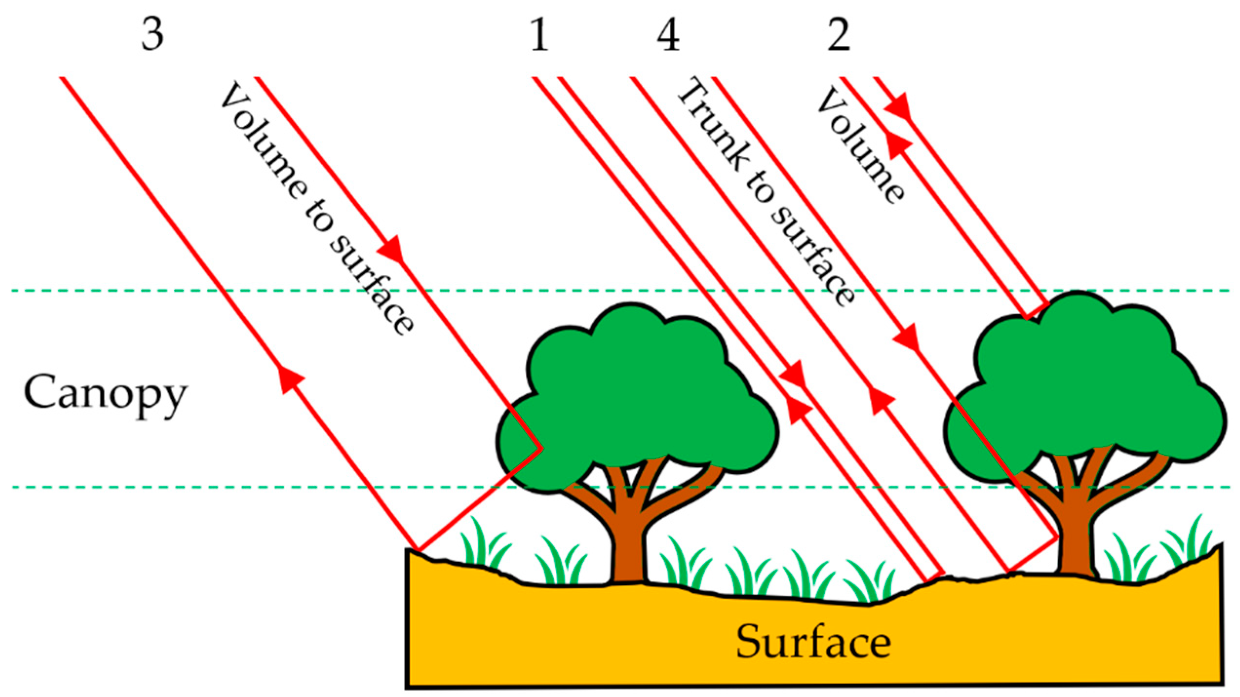
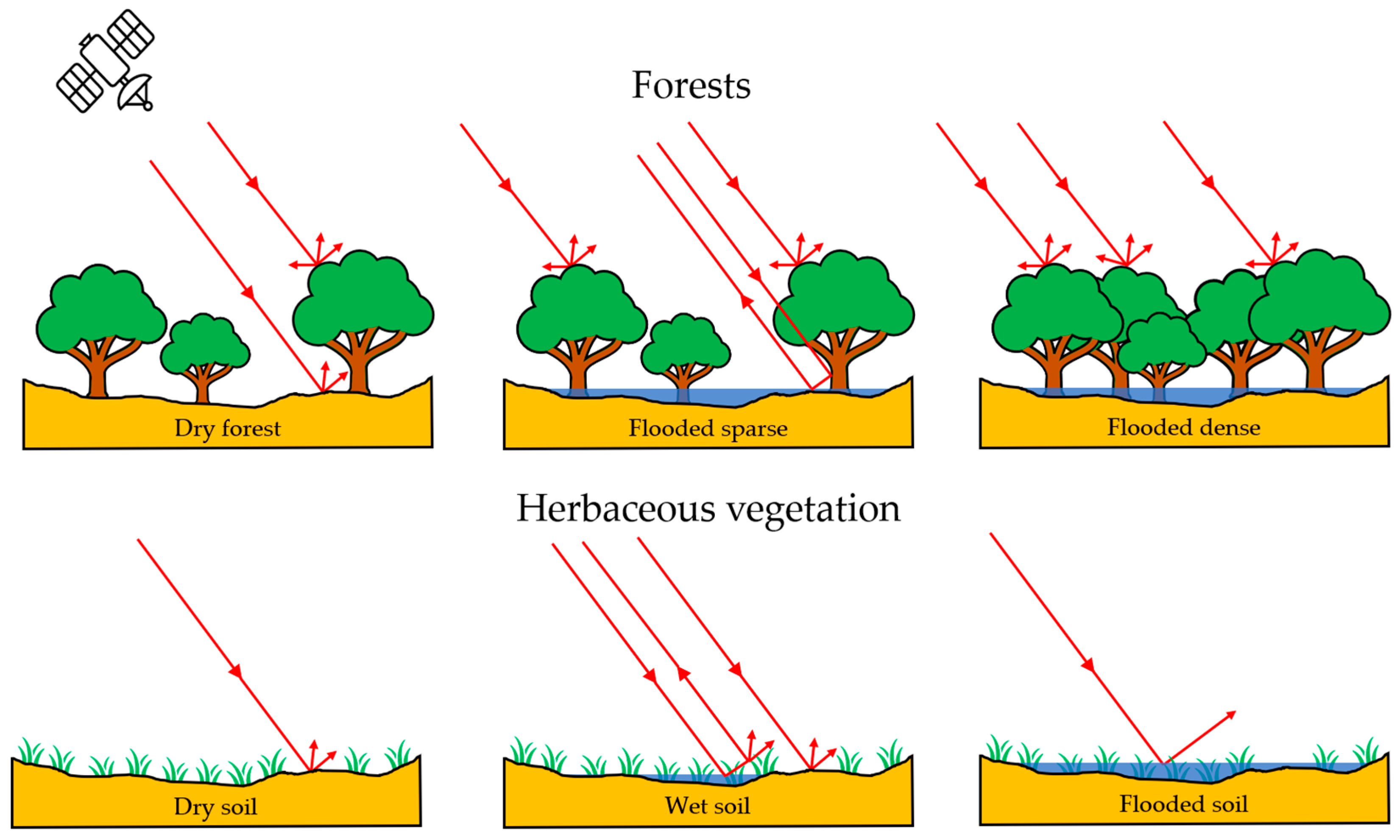
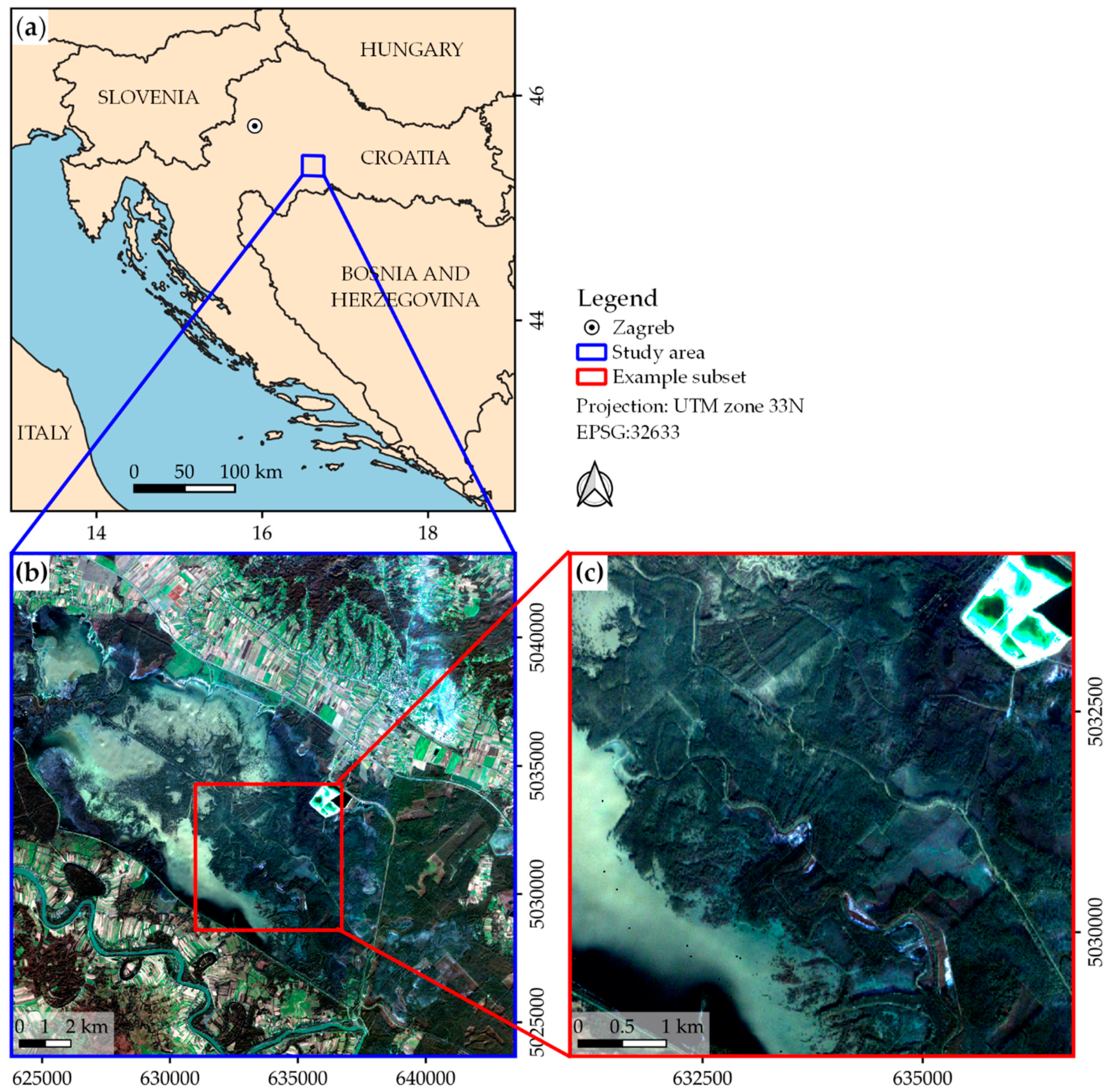
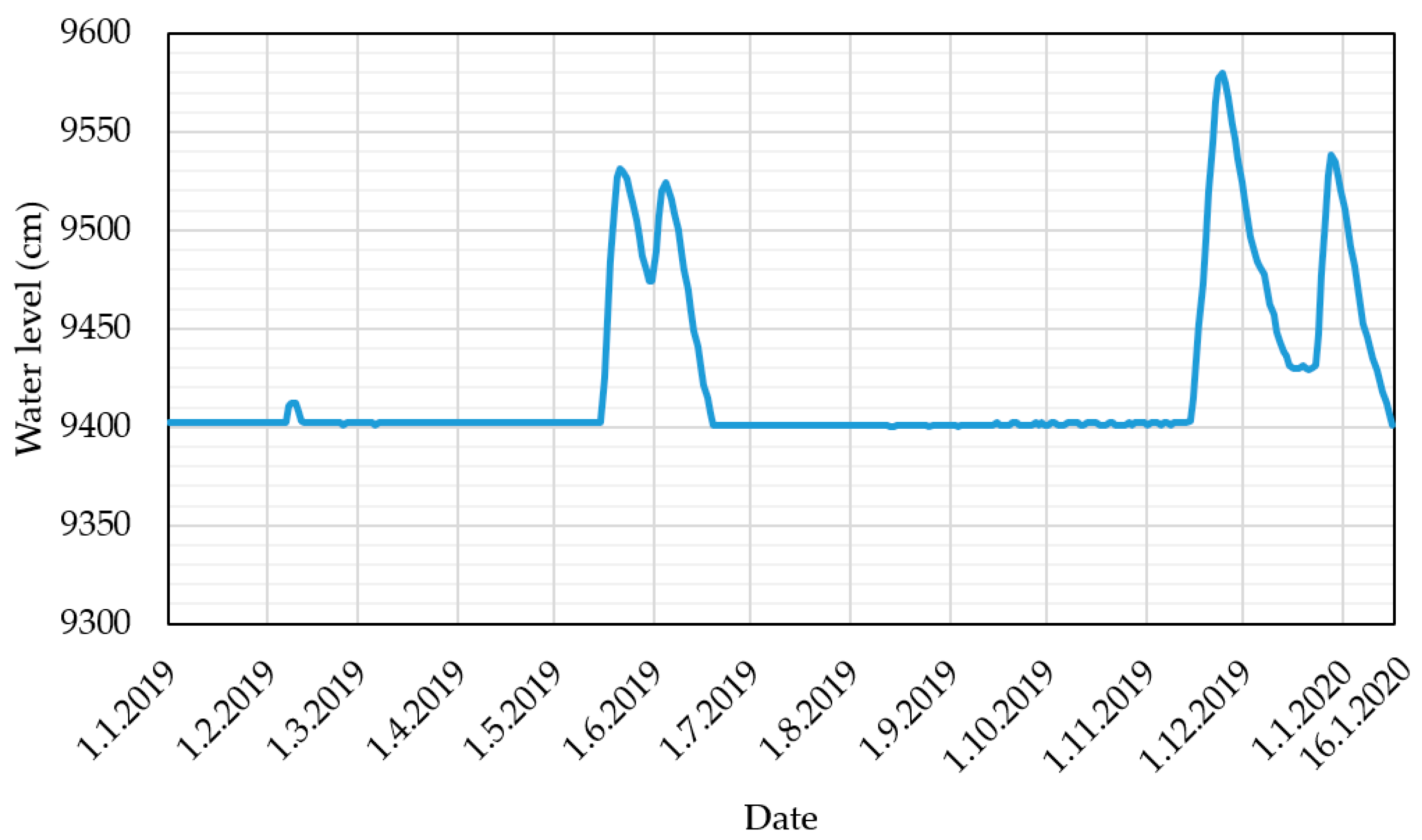
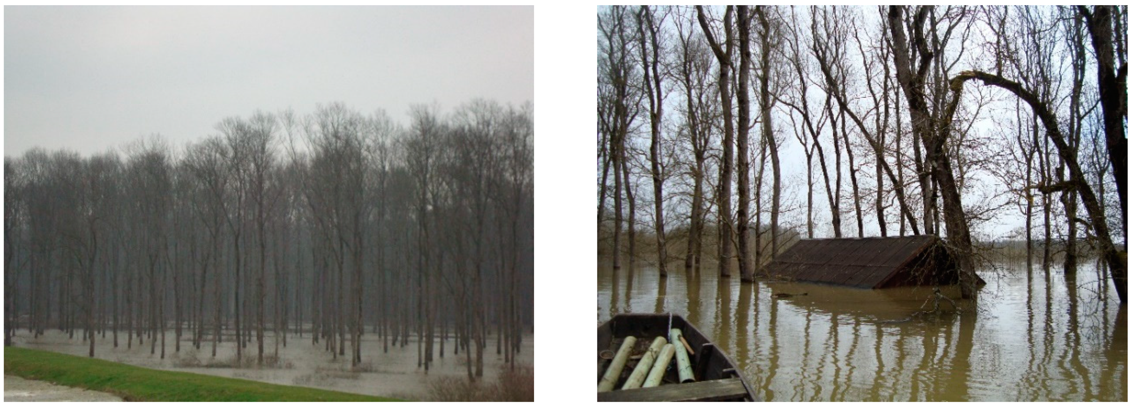
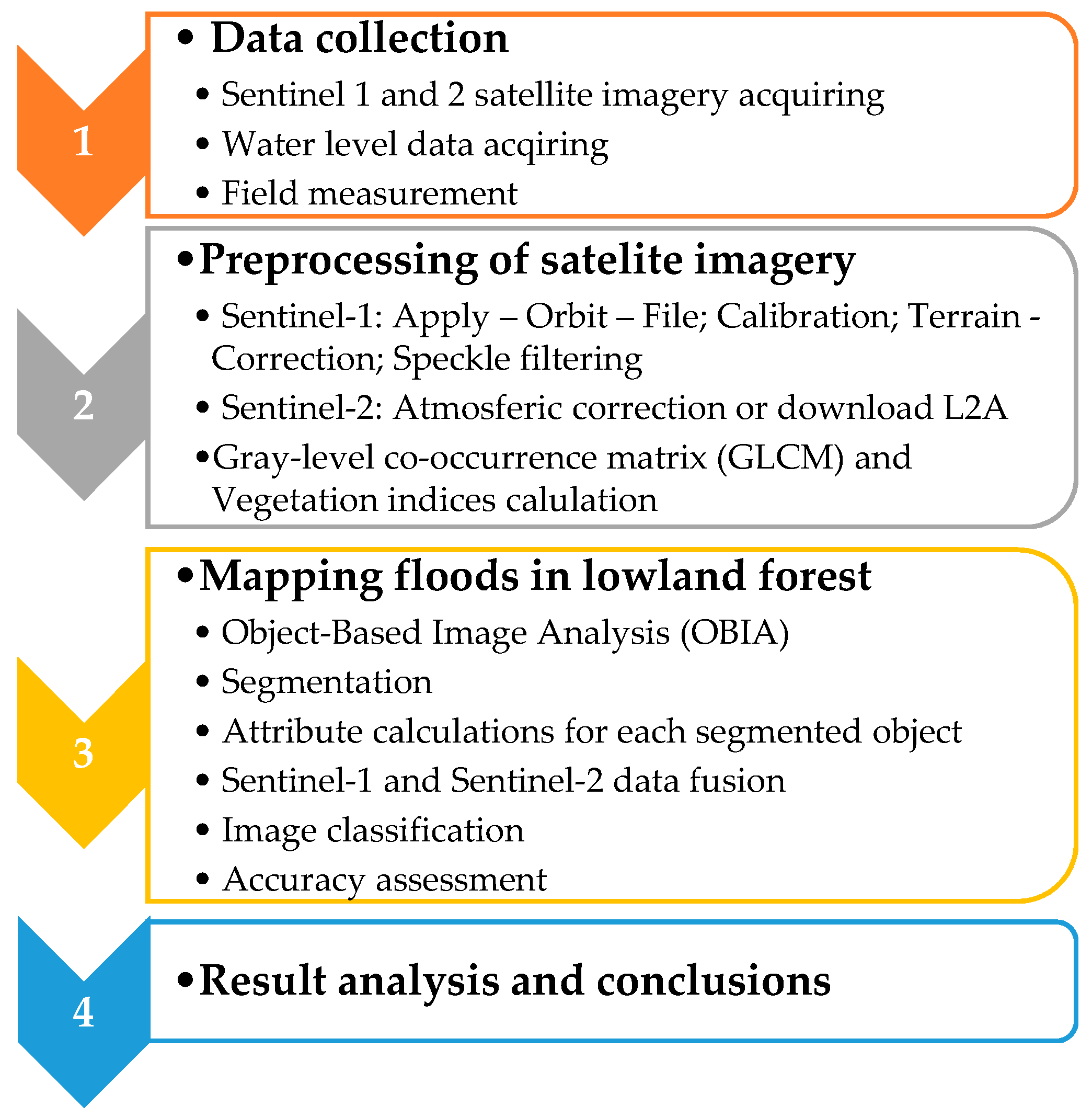
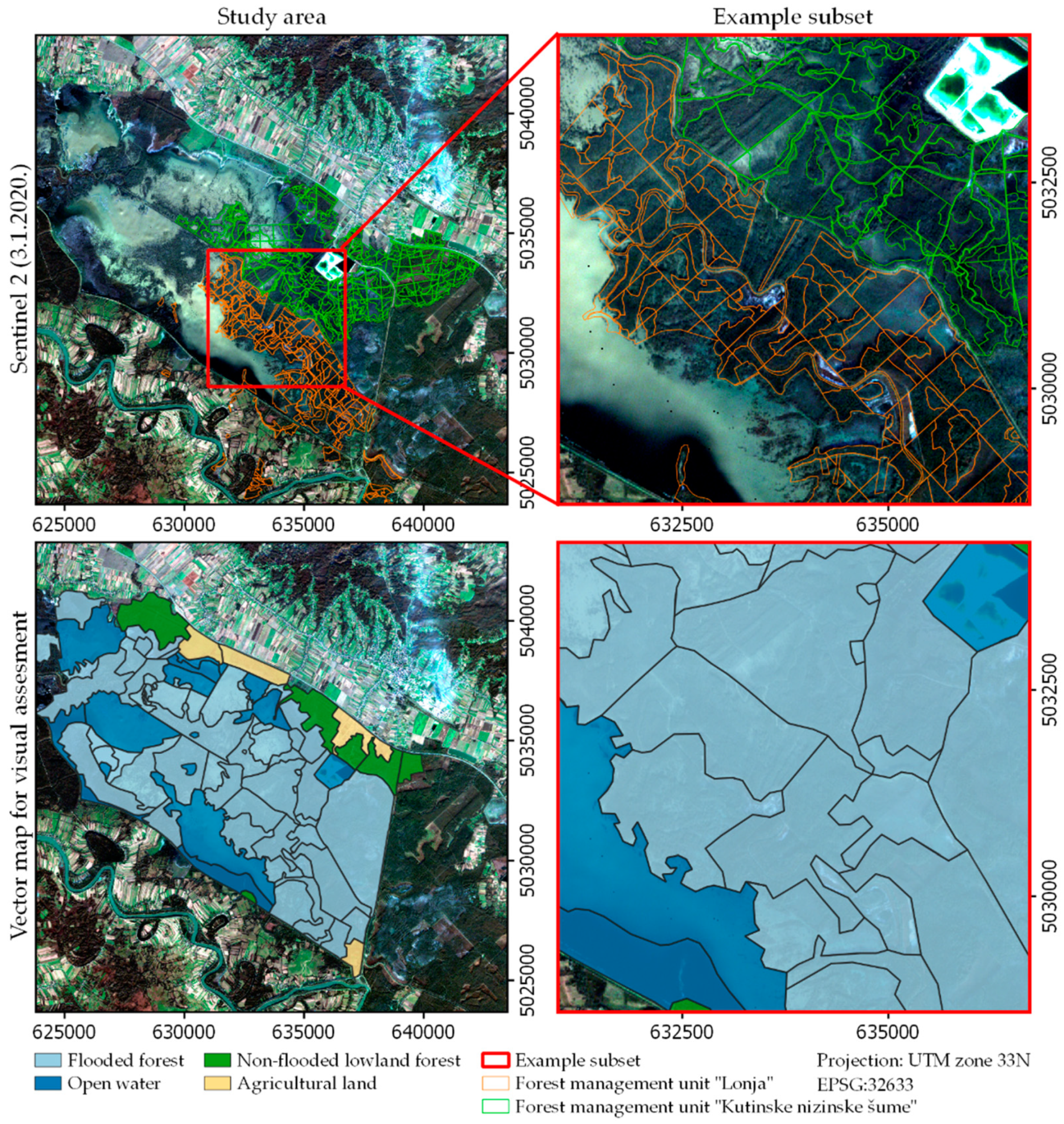
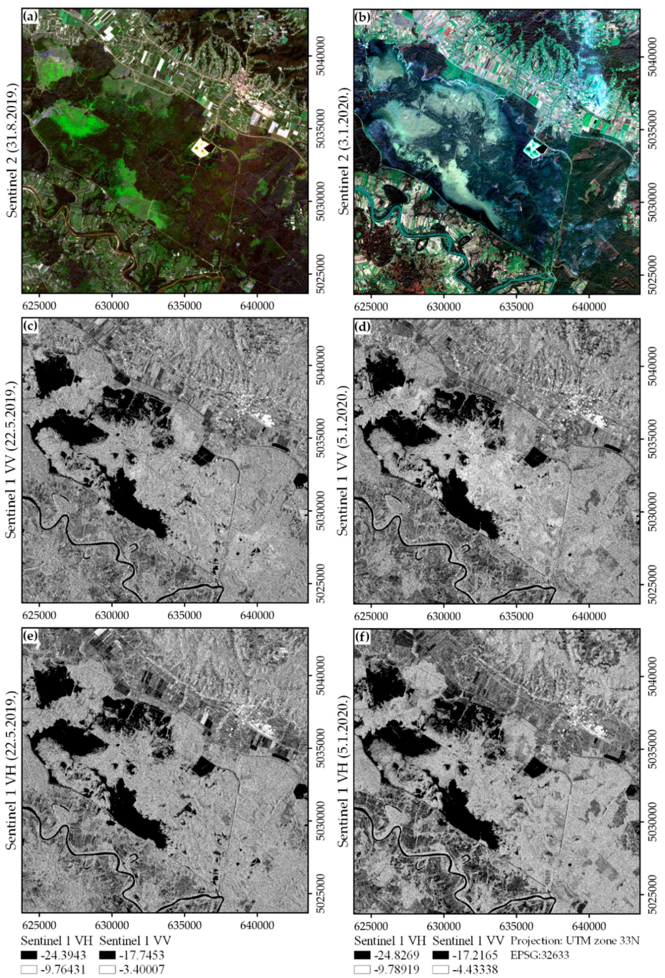
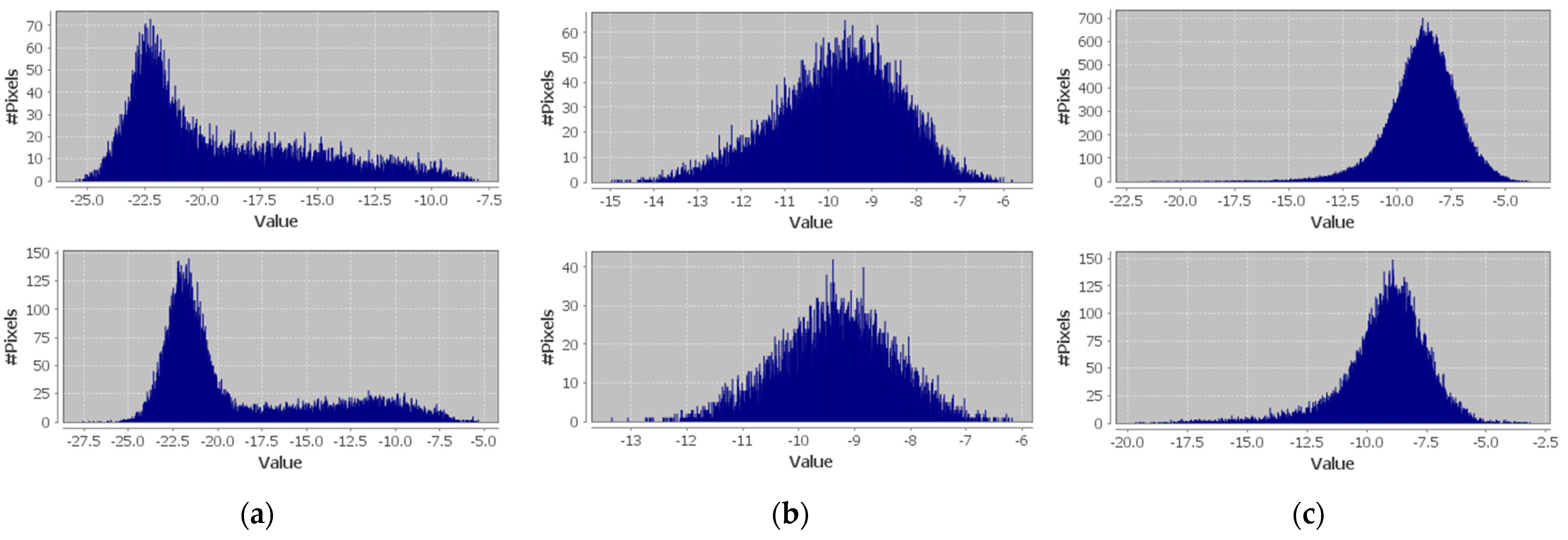
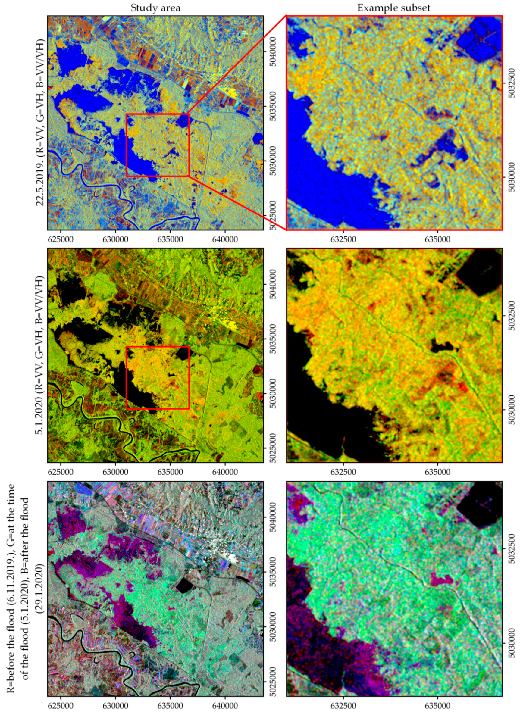
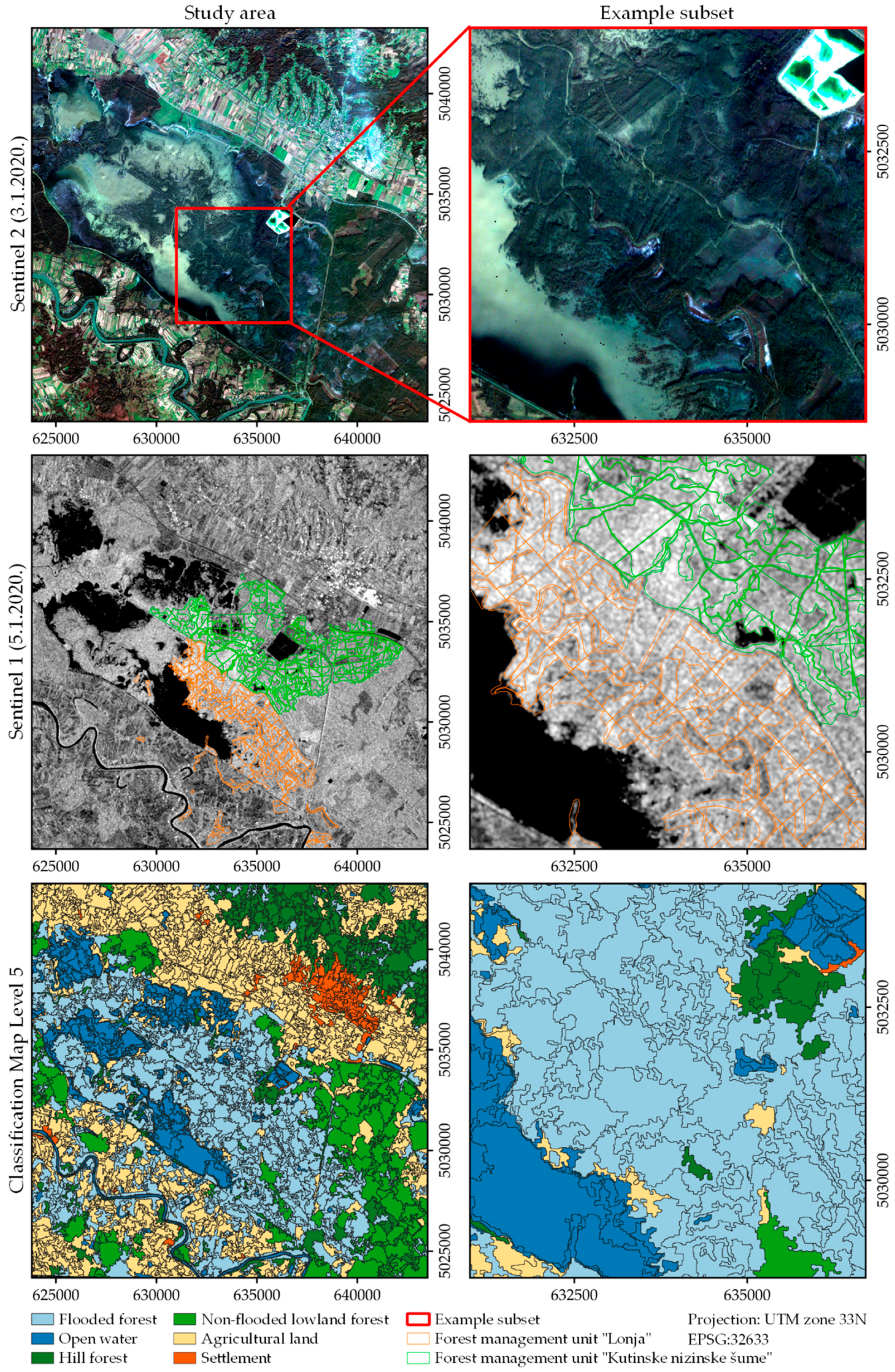
Table 1.
Relative scattering strength of individual bands by polarization [27].
Table 1.
Relative scattering strength of individual bands by polarization [27].
| Scattering Type | Polarization 1 |
|---|---|
| Rough Surface Scattering | |SVV| > |SHH| > |SHV| or |SVH| |
| Double-Bounce Scattering | |SHH| > |SVV| > |SHV| or |SVH| |
| Volume Scattering | |SHV| and |SVH| |
1 S = signal strength.
Table 2.
Satellite imagery metadata and purpose of use in the research.
| Sensor | Acquisition Date | Sensor Mode | Freq. Band | Spatial Resolution | Processing Level | Forest Condition | Purpose of Use |
|---|---|---|---|---|---|---|---|
| S1 | 22 May 2019 | IW/VV/VH | C | 10 m | GRD | Leaf on | Visual Assessment |
| S1 | 6 November 2019 | IW/VV/VH | C | 10 m | GRD | Leaf off | Visual Assessment |
| S1 | 5 January 2020 | IW/VV/VH | C | 10 m | GRD | Leaf off | Forest Flood Mapping |
| S1 | 29 January 2020 | IW/VV/VH | C | 10 m | GRD | Leaf off | Visual Assessment |
| S2 | 31 August 2019 | MSI | B2, B3, B4, B8 | 10 m | L2A | Leaf on | Forest Flood Mapping |
| S2 | 3 January 2020 | MSI | B2, B3, B4, B8 | 10 m | L2A | Leaf off | Visual Assessment |
Table 3.
Attribute calculations.
| Band/Indices | Statistical | Geometrical | Texture | Vegetation Indices |
|---|---|---|---|---|
| VV | ✓ | ✓ | ✓ | |
| VH | ✓ | ✓ | ||
| R | ✓ | ✓ | ||
| G | ✓ | ✓ | ||
| B | ✓ | ✓ | ||
| NIR | ✓ | ✓ | ||
| S2 (R, G, NIR) | ✓ | ✓ |
Table 4.
Vegetation indices used for attribute calculation.
| Indices | Equation 1 | Reference |
|---|---|---|
| GRVI | [74] | |
| NDVI | [68] | |
| SAVI | [77] | |
| MCARI2 | [69] |
1 In equations, G represents Sentinel-2 B3, R B4, and NIR B8, respectively.
Table 5.
Flood mapping classification approaches (levels) and used attribute calculations.
| Level | Band/Attribute |
|---|---|
| 1 | VV (Statistical, Geometrical) |
| 2 | VV (Statistical, Geometrical) + VH (Statistical) |
| 3 | VV (Statistical, Geometrical) + VH (Statistical + Texture (VV, VH, R, G, B, NIR) |
| 4 | VV (Statistical, Geometrical) + VH (Statistical) + Texture (VV, VH, R, G, B, NIR) + Vegetation Indices |
| 5 | VV (Statistical, Geometrical) + VH (Statistical) + Texture (VV, VH, R, G, B, NIR) + Vegetation Indices + S2 statistical (R, G, B, NIR) |
Table 6.
Descriptions of the forest geographical information system (GIS) layers.
| Name of the GIS Layer | Description (Reasons for Use) |
|---|---|
| Stand Class | Spatial distribution of forest and forestland (at stand level) according to the primary purpose of the forest, silviculture form, and main species of trees. |
| Age Class | Spatial distribution of stand by age classes. Age class width: 5, 10, or 20 years, depending on the stand class. |
| Density | Density is the most frequently used parameter in the quantitative description of stands. Relative density was used in the paper. The relative density is determined by the measured density (absolute basal area) ratio and standard (ideal) density from yield tables. |
Table 7.
Class description.
| Class ID | Class Name | Description |
|---|---|---|
| (A) | Flooded Forest | Lowland mostly mixed forests of pedunculate oak, narrow-leaf ash, alder and other accompanying species. The stands are of different age class, density, and site quality. |
| (B) | Open Water | Flooded grassland and unstocked timberland covered with lush herbaceous weeds and shrubs and individual or groups of trees. River and individual artificial water surfaces. |
| (C) | Unflooded Lowland Forest | Lowland forests outside the flooded area. |
| (D) | Hill Forest | Surrounding hill forests. |
| (E) | Settlement | Urban or larger rural areas. |
| (F) | Agriculture Land | Agricultural land. |
Table 8.
Training and reference data polygons used in classification.
| Class ID | Number of Polygons (n) and Area (ha) | % T in the Class Data | ||||
|---|---|---|---|---|---|---|
| Training Data (T) | Reference Data | |||||
| n | Ha | n | ha | n | ha | |
| (A) | 35 | 1382 | 19 | 862 | 0.65 | 0.62 |
| (B) | 35 | 846 | 11 | 249 | 0.70 | 0.77 |
| (C) | 22 | 1437 | 10 | 832 | 0.69 | 0.63 |
| (D) | 20 | 587 | 15 | 482 | 0.57 | 0.55 |
| (E) | 10 | 174 | 7 | 90 | 0.59 | 0.66 |
| (F) | 42 | 1245 | 17 | 546 | 0.71 | 0.70 |
| Total | 164 | 5671 | 79 | 3061 | 0.67 | 0.65 |
Table 9.
Overall statistic values for all levels of the object-based image analysis (OBIA) maps.
| Overall Statistics | Level 1 | Level 2 | Level 3 | Level 4 | Level 5 |
|---|---|---|---|---|---|
| Overall Accuracy (%) | 72.15 | 77.22 | 87.34 | 89.87 | 94.94 |
| 95% Confidence Interval | 61.63 | 67.33 | 79.38 | 82.59 | 89.47 |
| 82.67 | 87.10 | 95.31 | 97.16 | 100 | |
| Overall Kappa Statistic | 0.66 | 0.72 | 0.84 | 0.88 | 0.94 |
| Quantity Disagree (%) | 20.25 | 15.19 | 10.13 | 7.60 | 5.06 |
| Allocation Disagree (%) | 7.60 | 7.60 | 2.53 | 2.53 | 0 |
| Percentage Improvement of Overall Accuracy | - | 1.07 | 1.13 | 1.03 | 1.06 |
| Total Percentage Improvement of Overall Accuracy | - | 1.32 | |||
Table 10.
Confusion matrix for Level 5.
| Classified Class | A | B | C | D | E | F | Σ User | UA % | Kappa |
|---|---|---|---|---|---|---|---|---|---|
| Flooded Forest (A) | 19 | 0 | 1 | 1 | 0 | 0 | 21 | 0.90 | 0.87 |
| Open Water (B) | 0 | 11 | 0 | 0 | 0 | 0 | 11 | 1.00 | 1.0 |
| Unflooded Lowland Forest (C) | 0 | 0 | 9 | 0 | 0 | 0 | 9 | 1.00 | 1.0 |
| Hill Forest (D) | 0 | 0 | 0 | 13 | 0 | 0 | 13 | 1.00 | 1.0 |
| Settlement (E) | 0 | 0 | 0 | 0 | 6 | 0 | 6 | 1.00 | 1.0 |
| Agriculture (F) | 0 | 0 | 0 | 1 | 1 | 17 | 19 | 0.89 | 0.87 |
| Σ Producer | 19 | 11 | 10 | 15 | 7 | 17 | 79 | ||
| PA (%) | 1.0 | 1.0 | 0.90 | 0.87 | 0.86 | 1.0 | |||
Publisher’s Note: MDPI stays neutral with regard to jurisdictional claims in published maps and institutional affiliations. |
© 2021 by the authors. Licensee MDPI, Basel, Switzerland. This article is an open access article distributed under the terms and conditions of the Creative Commons Attribution (CC BY) license (https://creativecommons.org/licenses/by/4.0/).
Share and Cite
MDPI and ACS Style
Gašparović, M.; Klobučar, D. Mapping Floods in Lowland Forest Using Sentinel-1 and Sentinel-2 Data and an Object-Based Approach. Forests 2021, 12, 553. https://0-doi-org.brum.beds.ac.uk/10.3390/f12050553
AMA Style
Gašparović M, Klobučar D. Mapping Floods in Lowland Forest Using Sentinel-1 and Sentinel-2 Data and an Object-Based Approach. Forests. 2021; 12(5):553. https://0-doi-org.brum.beds.ac.uk/10.3390/f12050553
Chicago/Turabian StyleGašparović, Mateo, and Damir Klobučar. 2021. "Mapping Floods in Lowland Forest Using Sentinel-1 and Sentinel-2 Data and an Object-Based Approach" Forests 12, no. 5: 553. https://0-doi-org.brum.beds.ac.uk/10.3390/f12050553
Note that from the first issue of 2016, this journal uses article numbers instead of page numbers. See further details here.