Estimating the Service Life of Timber Structures Concerning Risk and Influence of Fungal Decay—A Review of Existing Theory and Modelling Approaches

Abstract

Wood is a renewable resource and a promising construction material for the growing bio-based economy. Efficiently utilising wood in the built environment requires a comprehensive understanding of the dynamics regarding its usability. Durability is an essential property to consider, as various types of exposure create conditions for the deterioration of wood through biotic and abiotic agents. Biodegradable materials introduce increased complexity to construction and design processes, as material decomposition during a structure’s lifetime presents a physical risk to human health and safety and costs related to repairs and maintenance. Construction professionals are thus tasked with utilising wooden elements to accentuate the material’s beneficial properties while reducing the risk of in-service decomposition. In this paper, only the cause and effect of fungal induced decay on the service life of wooden buildings and other wood-based construction assets are reviewed. The service life of wood components can thus be extended if suitable growing conditions are controlled. Multiple existing modelling approaches are described throughout the text, with special attention given to the two most comprehensive ones; TimberLife and the WoodExter. In choosing an appropriate model for a specific application, the authors recommend evaluating the model’s regional specificity, complexity, practicality, longevity and adaptability.

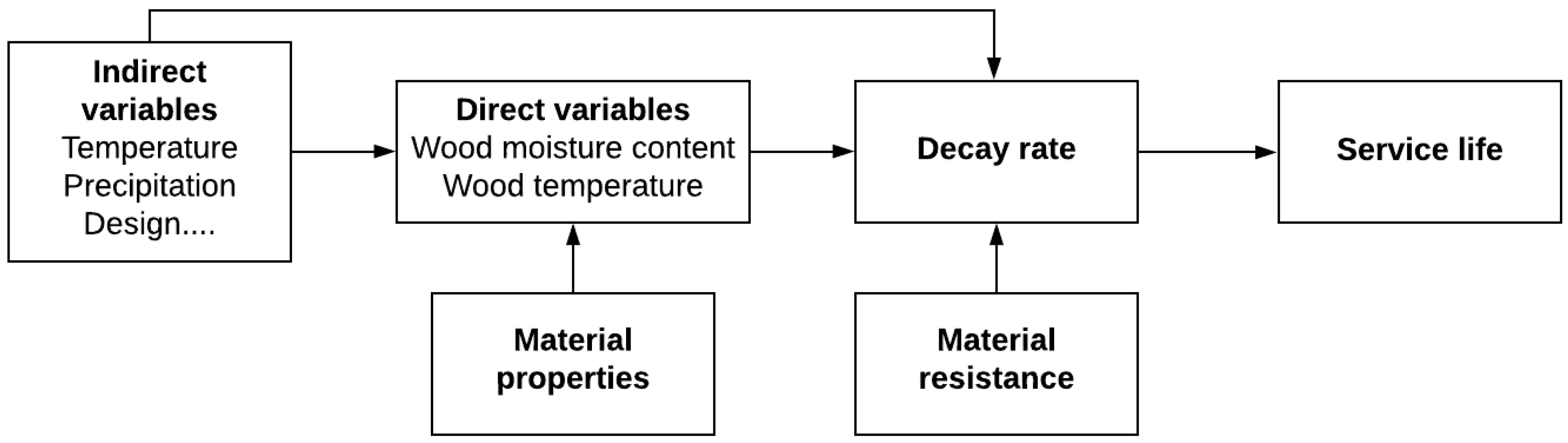
1. Introduction

Standards and policies are pushing construction professionals to apply a more holistic approach to building design and construction. To this end, the International Organization for Standardization (ISO) recommends a design process called service life planning (SLP). ISO 15686-1; 2011 [1] defines SLP as “a design process that seeks to ensure that the service life of a building or other constructed asset will equal or exceed its design life”. Service life (SL) in this context refers to the period from installation until failure—once a building element fails to meet its performance level requirements. As such, performance-based design (PBD) is becoming critical in ensuring that the required SL of buildings and construction assets are met [2,3]. Today, the construction industry is also looking to integrate environmental impact mitigation, which promotes the use of renewable construction materials. As a result, wood, which has been utilised as a construction material throughout human history, has become more appealing in modern-day construction [4].

A challenge with using PBD is that the computationally intensive nature introduces increased complexity to design procedures compared to conventional prescriptive design practices. Added complexity stems from its reliance on various mathematical equations, which are laborious and subject to a varying degree of human input. Utilising the computational power of the digital landscape, however, presents a solution to this problem. Building information management (BIM), for instance, already presents a platform that facilitates PBD. However, to successfully incorporate SLP into the digital landscape, information about wood material properties and its behaviour to environmental conditions will have to be integrated into a software framework. Information on wood performance as a construction material is available throughout scientific literature, especially in the form of written construction guidelines [5,6,7,8,9].

Additionally, attempts have already been made to transfer this information and knowledge into the digital landscape. Currently, two SL estimating software tools exist; Timberlife, an open-source educational tool created for the Australian environment [5], and WoodExter, an excel-based tool designed for the European environment [7]. This integration of various forms of SL modelling to software applications has much potential and room for growth and improvement. For instance, possible uses of SLP expressed by ISO include the ability to aid in experimentation and decision making concerning specifications and design detailing, life-cycle cost analysis, value engineering and maintenance planning [1]. The Intergovernmental Panel on Climate Change (IPCC) [10] also encourages carbon accounting practises for harvested wood products, and SL prediction models have the potential to contribute significantly to this goal.

The finite nature of biological materials like wood results from decay processes that degrade the material, ultimately recycling the elemental constituents [11]. Exposure to ambient moisture, temperature, solar radiation, strong acids, strong bases, oxidising agents, organic solvents and physical wear instances cause material decay directly or at least influence the material climate [11,12,13]. These factors are generally associated with certain use conditions and induced through particular decay agents. To practically model wood decay, models incorporate these two aspects, which allows for the isolation and grouping of specific mechanisms, while limiting exposure conditions [12,14]. In the case of this review, the influence of decay fungi as a decay agent is isolated, and use conditions are only expressed in terms of fungal decay hazard (

Table 1. A simplified version of the ISO 21887 [15] and EN 335 [14] use classification of wood and the risk of fungal decay.

Use Class ISO 21887	Use Class EN 335	Occurrence of Fungi
(1) Interior, dry	(1) Interior, dry	No hazard
(2) Interior, damp	(2) Interior, possibility of moisture condensation	Ubiquitous hazard
(3.1) Exterior, above ground, protected from the weather (3.2) Exterior, above ground, unprotected from the weather	(3.1) Exterior, above ground, weathering, limited wetting (3.2) Extended wetting	Ubiquitous hazard
(4.1) In-ground (4.2) In-ground, severe, fresh water	(4) Exterior, in ground contact and/or fresh water	Ubiquitous hazard
(5) Marine	(5) Permanently or regularly submerged in salt water	Ubiquitous hazard

).

Furthermore, only fungi that influence seasoned wood fall within the scope of this review. The classification of use conditions illustrated in Table 1 presents a framework of decay hazard influenced by factors like sheltering, local humidity levels and contact with precipitation, soil or free water [15]. Mainly, it attempts to categorise regions of the wood–water interaction since fungi are reliant on ample moisture in its environment. This will be discussed in more detail in later sections.

This review aims to supply modellers and software developers with a toolkit to model the cause and effect of fungal decay on timber components, for ultimate use in simulation and integrated software packages. Fungal decay is isolated, as its influence on SL has been studied the most extensively. In the review, state-of-the-art in SL modelling theory is discussed—firstly, on modelling the material climate followed by the modelling of decay. Furthermore, the characteristics of different fungi are described, focusing on the aspects relevant to SL modelling. The main focus is on the cause and effect of decay, the mechanism of decay and relevant life cycle processes. Lastly, suggestions are made to improve SL modelling, and existing approaches and frameworks are described and reviewed.

2. Fundamentals in Modelling the Behaviour of Decay Fungi

The role of fungi as recyclers of organic materials are critical to natural ecosystems [16]. Numerous species of these organisms have developed complex and sophisticated strategies to degrade and digest various compounds that make up wood [17,18]. A unique identifier of these organisms is their ability to penetrate, invade, externally digest and absorb soluble constituents [11]. Unfortunately, the activity of fungi does not stay confined to natural ecosystems, often leading to economic damages to human-made structures [19]. Furthermore, wood used in terrestrial, subterranean or aquatic environments often needs different durability requirements and strategies in modelling due to different boundary conditions and the presence of different fungal flora. Saprobes are fungi that specifically decay dead organic matter and plant debris. Fungi under this classification have been identified as the primary agent that influence the SL period of buildings and construction assets [20]. Three different groupings colonise seasoned wood, namely staining fungi, mould fungi and decay fungi.

The principle behind modelling the risk and influence of fungal decay is to incorporate aspects of the life-cycle and environmental requirements. For the growth and development of fungi, certain conditions regarding moisture and other physicochemical parameters like pH, oxygen, temperature and nutrients are required [21,22]. Due to the ecological scale of these organisms, environmental conditions also need to be scaled accordingly. For instance, the environmental conditions in and directly around a timber component present a habitat to the colonising fungi. As such, the conditions of the macroenvironment do not directly influence the fungi, but can indirectly influence the climate inside the woody material. In practice, direct variables, like material temperature and moisture content (MC), have proven to be useful in assessing decay development [23]; however, these variables are not frequently captured and are practically challenging to derive, as they depend on both the external environmental conditions and the properties of the wood. Therefore, some models recommend the use of indirect variables, which, in contrast to direct variables, are independent of the material at hand. Indirect variables utilise the indirect causality between macroclimate, local climate, design and decay rate. Figure 1 is a concept introduced in [24] that was later implemented by [9]. The concept illustrates how direct or indirect variables can be used to estimate SL ultimately. Additionally, Figure 1 acts as a framework that depicts the content that will be discussed further.

2.1. Moisture in the Material

The amount of moisture found inside wood is termed MC, which is commonly expressed as a function of the material’s dry mass. The influence of wood MC on fungal decay is possibly the most extensively investigated [21,22]. Zabel and Morrell [21] summarised the four critical functions of water to wood-decaying fungi as; (1) a reactant during hydrolysis, (2) a diffusion medium for solubilised substrate molecules and enzymes, (3) a medium or solvent for life systems and (4) a wood-capillary swelling agent. Wood is a hygroscopic material that frequently interacts with environmental moisture, continually tending towards equilibrium with its surroundings. Moisture uptake (adsorption) and release (desorption) are referred to collectively as sorption. Sorption behaviour is influenced by factors such as material ultrastructure and composition, and temperature and the vapour pressure of the immediate environment [25,26]. Additionally, moisture behaviour differs for moisture uptake and release due to the hysteresis between adsorption and desorption isotherms [26,27]. Moisture exists in wood in three different phases: (1) as bound water, (2) as water vapour and (3) as liquid water [26]. Bound water is chemically bound to the cell walls through hydrogen bonding, whereas water vapour and liquid water exist within the cell cavities. Existing models have assumed that the minimum moisture threshold (MMThr) for decay is the state when free water is available in the cell lumens [3,23,28,29]. It has been suggested that free water is required as fungi lack enough suction strength to remove bound water from wood cell walls [22,28].

For simplicity, free-water in the cell-lumens has long been assumed to only occur after a static MC value representing cell-wall saturation (CWS), commonly referred to as the fibre saturation point (FSP). That is, the binding sites of the polymer matrix need to be saturated first before free liquid water becomes available in the cell lumens. Alternative to MC, Griffin [30] used water potential to express the relationship and suggested that wood’s water potential needs to be about 0.3 g g⁻¹ before rotting fungi can access free water. Moreover, the critical water potential requirements determined by Griffin [30] are difficult to measure and correlates well with the moisture state of CWS. As such, models have commonly accepted 25% MC [23,31] or 30% MC [28] as a reasonable MMThr. However, the simplification of using a static CWS value is being challenged in recent years [22,26]. The reason being that the material MC at which liquid free-water occurs is strongly influenced by wood species and the substrate’s moisture history [22,32]. Additionally, moisture gradients inside the material and moisture traps can lead to localised CWS [33]. In attempting to model fungal growth and decay, the use of the theory that free water only occurs post-CWS might thus be an oversimplification, especially when only a universal and static threshold value is used.

Fundamentally, the state of importance is the conditions when water in the polymer matrix comes in contact with fungal hyphae and becomes available to the passive osmotic capabilities of the said hyphae [21,30]. However, this state should be determined locally as MC distribution is variable across a wooden element at any point in time. For instance, moisture migration from the boundary to the material’s interior, resulting specifically from free-water contact might temporarily produce localised suitable conditions as the surface water migrates. If the fungi happen to be in the moisture migration path, some moisture could become subject to the osmotic capabilities of resident fungi or germinating spores. As a result, free-water contact has proven to be a significant driver of fungal development. Scheffer [34], for instance, had much success in using precipitation events as variables in the Scheffer climate index (SCI), while others [31,32] reported on strong correlations between decay development and events that result in free-water contact.

Another material moisture state exists that can be a candidate for an MMThr of fungal decay. Jakes et al. [35] suggest that different wood species undergo glass-transition at specific MC and temperature combinations. As a result, the water and enzyme diffusion mechanism is slower for a polymer matrix in a rigid glassy state than for the same material in a soft rubbery state. Thus, a rigid glassy state inhibits the ability of the fungi to distribute enzymes effectively. Glass-transition occurs at a lower MC than CWS, meaning that during adsorption the state transition from glassy to soft rubbery occurs before CWS. Even though the glass transition threshold represents an adequate theoretical MMThr, its influence has not been investigated to the same extent as the presence of free water.

As water becomes more abundant in the material beyond CWS, the fungal growth rate increases with increased amounts of free water. However, this relationship reaches a cardinal tipping point from which increases in free water will decrease the growth rate. The tipping point would theoretically represent the moisture optimum for growth; however, the exact point of these moisture conditions is mostly unknown [21]. The moisture optimum and the maximum moisture limit are influenced by the material’s oxygen content. Excess amounts of free water displace oxygen to such a degree that the environment in the substrate turns too oxygen-deficient for the wood-inhabiting fungi [12,28,36]. Most decay fungi are aerobic, which means that the anaerobic conditions restrict important life systems of the fungi as they require oxygen for several metabolic reactions [21]. The wooden ultrastructure and composition strongly influence the water–oxygen ratio under different moisture loads, and the exact threshold for oxygen deficiency is subject to the fungi species and its oxygen requirements.

2.2. Temperature Conditions

Multiple metabolic reactions of fungi are directly affected by temperature [21]. As for material MC above, a minimal, optimum and maximum condition can be defined for temperature as well. Established models generally use a temperature range of 0–40 °C [23,28,29]. Psychrophilic and thermophilic species can still grow and develop outside this range, while sustained temperatures higher than 60 °C are deemed to be fatal to most decay fungi species [21,28]. A range of 0–40 °C is thus appropriate as a general range for most wood-inhabiting fungi, which are mesophilic. Moreover, temperature curves indicating minimum, optimum and maximum conditions vary significantly among and within fungi species [21].

Other than species-specific minima, a general cardinal temperature threshold is the freezing point of liquid water. Water in solid form becomes unavailable to fungi, ultimately inhibiting the mode of action (MOA) regarding water and enzyme diffusion. It is well-known that distilled water freezes at 273.15 K (0 °C) at atmospheric pressure. Inside wood, however, undercooling of free water is possible [37]. Engelung et al. [26], for instance, suggest that dissolved sugars can lead to a slight freezing point depression, and further explain that the proximity of free water to cell walls strongly influences the freezing point [37,38]. It thus becomes apparent that for most decay influencing processes temperature, MC, oxygen and the polymer structure are interdependent. For instance, temperature also affects sorption behaviour and glass transition. As such, the combined use of moisture availability and temperature has already shown much promise in a modelling context [23,28,29,34,39].

3. Collection and Determination of Material Climate Variables

With the importance of material climate already stated, the next important step is to discuss all the possible ways of collecting these variables. Localised measurements need to be non-destructive in order to collect adequate time-series information. As such, monitoring devices like in-situ sensors are commonly used. Embedded electrodes that measure electrical resistance have been successfully used in construction to capture and monitor MC behaviour, especially in historical and high valued structures [40,41]. The use of electrical resistance measurements is also commonly incorporated in research [32,42,43,44]; however, electrical resistance becomes less efficient at translating to MC at higher levels of free water, leading to decreases in measurement accuracy [42,44]. Moreover, load-cells that monitor MC behaviour through mass changes have been incorporated in research [45] and relative humidity (RH) sensors that deliver in combination with temperature data the equilibrium moisture content (EMC) of wood [46].

Material moisture and temperature conditions are mostly a product of the ambient environment. In modelling, a reasonable expectation is that ambient air temperature will be the same as the wood temperature [24]. However, there are situations where this is not the case. For instance, solar radiation can cause higher temperatures at the surface, which creates a temperature gradient in the material. On the other hand, the surface might be colder than the environment due to radiative cooling. Additionally, to a lesser extent, the material can absorb or release heat energy internally during moisture desorption or adsorption. The process is referred to as the heat of sorption or sorption enthalpy [35]. Localised adsorption or desorption can thus lead to slight temperature differences between the ambient environment and material climate. Though, on a daily time scale, these influences are believed to be non-significant. Nevertheless, for localised measurements, temperature sensors in the form of thermocouple or a resistance temperature detector can be used to capture temperature information of the ambient climate or internal climate if embedded [47].

Direct or contact-based measurements like these have a few drawbacks, however. For one, installing the specific equipment is not practical for all timber buildings and building assets, making these variables less available. Additionally, as Figure 2 depicts, contact-based in-situ sensor measurements are spot measurements that can have difficulty with measuring spatial distribution. An alternative or supplementary approach could be to use remote or contactless in-situ sensors to capture material climate information over a larger section of a building (i.e., multiple components). Infrared thermography is one such technology that shows promise in detecting surface moisture while also having the capability to measure surface temperatures if the emissivity of the material is known [48,49]. Nevertheless, these sensors are also limited in their ability to monitor the material climate, as gradients inside the material stay undetected and critical design details like connection points are not fully captured.

3.1. Modelling the Material Climate

An alternative to measuring material MC and temperature is to model it from more abundant climate data. With this method, decay modelling becomes a two-step process (Figure 1), while the cost and effort associated with the installation of large amounts of sensors get eliminated. Weather stations present a readily available climate data source; however, the accuracy of the data at a particular location strongly depend on the proximity of stations. It is also common for weather datasets to utilise interpolation for regions between stations [2,50]. Macroclimate, mesoclimate and microclimate represent three degrees of scale in descending order. Macroclimate refers to the general climate of a large geographic area at the regional or national level, while the mesoclimate represents an intermediate geographic scale. A macroclimate can contain numerous mesoclimates, which usually represent different landscape types that are often influenced by terrain features and topography [51]. From the mesoclimate the geographical scale can further be reduced and separated into microclimates, for instance, representing different climate zones in and around a building. Ideally, the microclimate would present more robust input variables, as the scale is the closest to the material climate [29]. Unfortunately, data on direct measurements of the microclimate are scarce.

Of all the climate metrics, the ones of interest are the ones that influence the sorption behaviour of wood. Most research has looked at the influence of RH, ambient temperature and events that lead to free-water contact [2,45]. Van den Bulcke et al. [45] also referred to the influence of solar radiation and wind speed on the surface flux and ultimately desorption. One of the major causes of free water contact with wooden components in use class 3 (Table 1) is precipitation, with events leading to liquid water contact being the most significant. During precipitation events, free water contact from wind-driven rain and splash water should also be taken into consideration [12,29]. Free water contact can also stem from condensation, leaks in sheltering structures or artificial wetting events [9,24]. With in-ground conditions, the moisture exchange will depend on the surrounding substrate or medium and its hydrological properties, while for fresh water or marine environments, free-water contact is semipermanent to permanent [5,52].

Within a structure, different regions experience different degrees of exposure to the climate parameters mentioned above. Building overhangs are good examples of design features that influence multiple climate parameters. Other components in an area below it mostly get sheltered from precipitation and solar radiation; however, the degree of exposure inhibition is influenced by the overhang design regarding its size, shape, orientation and position in the structure [43]. Additionally, in above-ground situations, ventilation is a significant driver of moisture exchange. A lack of ventilation has been found to lead to elevated moisture levels in wooden components, often observed around inter-component connection points or cracks that create moisture traps [9,33,44].

Lastly, the intrinsic material properties also play a major role in the way the material reacts to its environment. Material intrinsic properties include the number of tyloses, blocked pits, wood relative density and other matrix characteristics like void space; and the distribution, amount and type of extractives present in the material [12,27,53]. Different sorption properties can thus be expected for different wood species, and between different sections of the stem (e.g., heartwood and sapwood). Moreover, differences in these properties can also be attributed to growing location and the time of harvest [12,54]. Additionally, in the case of treated or modified wooden products, the treatment/modification type and its intensity can also influence the material’s sorption properties. The material’s sorption properties are altered by treatments or modification processes if water repellent agents are introduced into the material or when processes are used that influence the availability of free hydroxyl groups.

3.1.1. Numerical Models

As aforementioned, wood moisture exists in three different phases, either bound to the cell wall through hydrogen bonding or in the lumens as water vapour or liquid water. Transport of bound water and water vapour can both be described by Fick’s second law of diffusion where the rate of change is expressed as a function of the moisture gradient and a diffusion coefficient. In one dimension, it can be expressed by Equation (1):

$$\frac{dw}{dt}=\frac{d}{dx}\left(D_w\frac{dw}{dx}\right)$$

(1)

where w is the moisture concentration (kg/m³); D_w is the diffusion coefficient (m²/s). In the case of liquid water, transport is governed by Darcy’s law of fluid flow in porous media, where it is expressed as a function of the inherent permeability of the material and the pressure gradient. Combined with the equation for mass conservation, Darcy’s law can be expressed by Equation (2):

$$\frac{dw}{dt}=\frac{d}{dx}\left(\frac{K_s{\rho }_w}{{\mu }_w}\frac{dP}{dx}\right)$$

(2)

where K_s is the permeability of the wood (m²); ${\rho }_w$ is the density of water (kg/m³); ${\mu }_w$ is the viscosity of water (Pa ⋅ s); dP/dx is the pressure gradient (Pa/m).

In the absence of liquid water, i.e., in use-class 1 and 2 (Table 1), moisture transport has predominantly been modelled as a single-phase process (single-Fickian) where a single quantity collectively describes vapour and bound water. Discrepancies between the single-phase model and measured data [55] have led to the development of multi-Fickian models where the transport of bound water and water vapour are modelled explicitly [56,57]. The transport of liquid water has, however, not yet been integrated into the multi-Fickian theoretical framework. Since exposure to liquid water is a prerequisite for decay, the more advanced multiphase models are unsuitable for decay assessment, although they hold great potential for the future.

Single-phase models based on Fick’s second law of diffusion have also been used to model moisture transport in the over-hygroscopic region [33,58,59,60]. This is made possible through the capillary pressure being a function of liquid water content [61]. The part of the diffusion coefficient, which extends beyond the hygroscopic range is either derived from the permeability of the material (see, e.g., [58,60]) or measured directly under non-steady-state conditions [62].

While numerical models based on constitutive equations prove to be promising in determining material MC, there are also several limitations. For example, the single-phase model has mainly been used for modelling Norway spruce (Picea abies) [24]. The potential for applying the same method for modelling the MC of other wood species remains uncertain. Modelling end-grain absorption presents yet another challenge. Finally, the application of numerical models requires commercial software and a relatively long computational time, in particular when solving a two or three-dimensional problem, thus limiting its practicality and availability.

3.1.2. Empirical Models

Some attempts have been made to describe the relationship between MC and climate parameters using empirical models fitted to MC data sets. Frühwald Hansson et al. [2], presented a model fitted to data obtained from plywood specimens of various species. The same model has been used in durability applications, e.g., [63]. Niklewski et al. [24] modelled the effect of different details on MC using an approach where the change in MC was calculated on a daily basis from weather data. Accurately predicting the fluctuations of rain-exposed wood is challenging due to the time-lag partly between precipitation (cause) and the response of the material to the wetting instance (effect) [45].

4. Modelling Fungal Growth and Wood Decay

Globally, much research has been done on the development of fungi related models and their influence in the built environment. Recent reviews on this issue include a review of decay models by Brischke and Thelandersson [64] and a review of mould models by Vereecken and Roels [65]. Numerous models incorporate some combination of the direct or indirect input variables covered in the previous sections to model fungal growth and decay. However, formulating these variables in the form of a dosage has been a popular choice for numerous modern approaches [3,7,9,23,66]. The method stems from the concept of dose–response modelling, which was first introduced in the context of decay assessment by Brischke and Rapp [23]. In this context, dose represents a unitless metric of suitable conditions for fungi development, which elicits a response in the form of growth or decay progression. As such, SL can be expressed in terms of cumulative dose, which act as a damage function that can also be used to evaluate relative performance [24]. As used by Brischke and Rapp [23] and later on by Isaksson et al. [3], the dose is a direct function of the material climate that effectively integrates cardinal material climate conditions into a modelling framework. The minimum, optimum and maximum MC and temperature conditions described before are formulated in terms of dose in Figure 3. Another advantage of using dose in this sense is that it allows for time-series analysis while linking elements between exposure and resistance for PBD [3].

4.1. Fungi Life-Cycle Considerations

Fungi that interact with wooden components go through numerous life-cycle stages during the SL period. Brischke and Alfredsen [22] stated six different phases of importance: “(1) spore arrival, (2) spore germination, (3) mycelial growth, (4) wood metabolism, (5) autolysis of fungal hyphae and (6) formation of fruiting bodies and sporulation”. Each of these is assumed to have different moisture and physicochemical requirements. SL modellers have, however, further grouped these processes into two phases, namely an initial “lag phase”, followed by a period where fungi metabolise wood henceforth referred to as the “decay phase” [3,5,29]. Some modelling techniques use different functions to separate the two phases [3,28], while others prefer sigmoidal curves that are capable of modelling both phases in a single model [23,66]. A longer lag phase is observed in above-ground samples where pioneering events are mostly a result of spore germination and detoxification through so-called non-target organisms, i.e., non-decaying fungi and bacteria. However, when exposing specimens to developed hyphae, like in pure cultures or certain soil substrates, the onset of decay is much more rapid [67,68]. Here, the fungi have access to more resources while spore arrival and germination is not required.

Fundamentally, two different processes are being modelled by the two phases—the conditions required for the fungi to initiate decay, in the case of the lag phase, and loss of material in the case of the decay phase [29]. The accumulation of suitable conditions represents a reversible process, while material decay represents an irreversible process regarding the original material. The implementation of negative growth is thus only possible during the lag phase [3,29]. For fungi, negative growth results from the loss or self-digestion (autolysis) of the mycelium, which is exaggerated by prolonged periods of unfavourable conditions but should not be mistaken for negative wood decay.

4.1.1. Lag Phase—Establishment

Establishment in this context refers to the cumulative periods of suitable conditions required to initiate decay. In above-ground conditions, spores or hyphae fragments first have to arrive, and then develop gradually in suitable conditions while surviving on stored and freely available nutrients. During this time, the fungus mobilises to find an acceptable region where it then initiates decay [69]. Since spores are ubiquitous in the air, its probability of reaching wooden components is very high [20]. Spore moisture requirements and germination rates differ between fungal species, influencing the community role regarding the competition for the substrate [70,71,72,73].

On the other hand, colonisation through hyphae expansion can occur when attached hyphae of developed fungi come in contact with wooden components [22,74]. Wooden elements in contact with a substrate that facilitates hyphae movement, like soil, are prone to this type of colonisation. Additionally, in above-ground situations, wooden elements that experience different levels of decay inducing exposure can facilitate this type of colonisation from one to another. Practically, the behaviour of expanding fungi is much more challenging to model due to increased amounts of hyphae and mobility relative to germinating fungi. Established fungi networks can also translocate water and nutrients [21]. As such, a logical solution would be to try and separate the mode of colonisation in a modelling context. The use-class system (see Table 1), for instance, already aids in separating occurrences where wood could come in contact with soil and, in turn, established fungi.

As mentioned before, the growth of fungi can stagnate and even decrease during unfavourable conditions. Viitanen et al. [29] proposed a concept to include negative growth to exposure models by using “a rate of decrease” function during unfavourable periods. The concept holds promise, but as the authors explain, the actual function is not based on specific empirical data, but instead based on scattered information. Isaksson et al. [3] attempted to implement a similar approach to dose–response modelling, referred to as a set-back function; however, the adaptation did not improve the original model’s fit. The authors argue that the data set did not support the creation of such a function as the moisture trapping design did not create enough periods of unfavourable conditions. The nature of the data produced from a test set-up should thus be taken into consideration when attempting to implement this aspect to modelling approaches.

4.1.2. Decay Phase—Material Loss

Once established, the fungi initiate their respective methods of removing constituents from the material. The removal of components from the polymer matrix is referred to as decay or rot, which is the dependent variable in this stage of the modelling process (Figure 1). Decay fungi are defined as such as they degrade the major polymers of wood (lignin, cellulose and hemicellulose). The enzymes of these fungi depolymerise cell wall constituents into water-soluble molecular fragments that the fungi ultimately metabolise [16,75]. The onset of decay should be prevented in wooden components as the microstructure of the wood becomes altered [76], which leads to losses in mechanical properties [67,68,77,78]. Moreover, multiple other functional properties also become altered [76,79].

The process of decay is variable, as various fungi species utilise different strategies and decay mechanisms. Commonly in literature, decay fungi get categorised as either causing white rot, brown rot or soft rot. Species that cause soft rot generally belong to the Fungi imperfecti or Ascomycetes, while brown rot and white rot are caused most frequently by species from the phylum Basidiomycota [20,22]. It is important to note that rot categorisations do not define fungal taxa but rather functional outcomes and general decay mechanisms [22,80]. Additionally, even though the rot classification paradigm has become common in the last few decades, its delineation criteria have trouble grouping some species with complex decay mechanisms [18,22]. However, this system currently presents the best solution for grouping species in a modelling context and will be discussed further.

Three distinct decay patterns are predominant among decay fungi from the Basidiomycota phylum, namely brown rot, successive white rot and simultaneous white rot [69]. A characteristic of brown rot is the depolymerisation of polysaccharides (cellulose and hemicellulose) via oxidative mechanisms while leaving a residual modified mass of lignin [69,76,80,81]. Additionally, brown rot causes substantial strength loss during incipient decay [67,79,82]. Researchers argue that significant strength loss stems from this grouping preference for polysaccharides in the S2 layer while modifying the lignin without attempting to utilise it as a food source [16,69,81]. Brown-rot fungi have a progressive attack mechanism that starts from inside the cell lumens [17,69]. For example, Zhang et al. [75] were able to demonstrate the progressive mode of action (MOA) of a brown-rot species using a water and soil block test set-up. Their results suggest that Postia placenta uses more oxidation enzymes at the hyphal front, while polysaccharide hydrolysis enzymes become preferential as the hyphae mature. Macroscopically, brown rot causes a phenomenon called cubical fracture, which is the appearance of fractures in the form of rough cubes [16,69]. Additionally, cellulose removal causes the wood to discolour to a brown shade, leading to a general change in appearance [16,69,76].

White rot involves hydrolases that gradually degrade polysaccharides while also mineralising lignin [18,69]. White rot affects any wood type but is commonly associated with hardwood decay [32]. Macroscopically, white rot causes the wood to turn white or yellow and results in softened, spongy or stringy texture, and darker coloured zone lines may also appear [16,69]. During successive white rot, the three major polymers are degraded in stages, whereas simultaneous rot, as its name suggests, simultaneously degrades these polymers [69]. As both strategies significantly degrade lignin, the current binary classification categorises both under white rot. Researchers are, however, suggesting a shift in the current rot classification paradigm to more accurately incorporate the diverse mechanisms found amongst rot groupings [18,80].

Soft rot is the latest edition of the rot classification system. Fungal species in this grouping can colonise wood at conditions that are unsuitable for most white rot or brown rot species [69,74]. These fungi, however, often need exogenous nitrogen to decay wood [74,83], increasing the risk of soft rot decay in terrestrial environments or for elements in ground contact [40,52,69,84]. Soft rot has two distinct patterns of decay, referred to as type 1 and type 2 soft rot. For type 1, the fungi specifically target the S2 layer of cell walls, creating small holes or cavities that are rhombic or oval-lancetlike [17,74,85]. For type 2, on the other hand, the degradation results in the thinning and erosion of the S2 layer, with the absence of the characteristic cavities [85]. In advanced soft rot stages, full degradation of the secondary cell wall may occur, leaving the middle lamella intact. Macroscopic characteristics of soft rot are the formation of rectangular shrinkage cracks and a general darkening and softening of the surface [69].

4.1.3. Saprophytic Fungi Outside of the Rot Classification

The rot classification system is geared towards fungi that cause rot and decay, ultimately leading to mechanical property losses. Nevertheless, other groupings exist that influences SL in different ways. These species will briefly be discussed; however, their influences fall outside of this review’s scope, as different modelling strategies are generally required to evaluate their influence on SL. The species in question are referred to as staining fungi and mould fungi, which mainly feed on byproducts of the weathering process and starches and free sugars generally located in the parenchyma cells of the sapwood [17,86,87]. Mould can refer to species that grow on wooden surfaces that cause discolouration or species that release allergens that exacerbate allergic diseases. The latter is more of medical classification, and Li and Yang [88] have identified species that can cause allergic responses in the taxonomic groups Ascomycota, Basidiomycota and the Deuteromycota. Allergens can come in the form of spores, hyphae or fungal fragments. Inhalation of high doses of airborne allergens is subjectively associated with symptoms such as cognitive difficulties, fatigue or memory loss, and more definable diseases such as asthma, allergy and hypersensitivity pneumonitis [6,89].

Moulds and mildews that lead to surface discolouration are also an aesthetic concern. Discolouration does not result from hyphae penetration as their hyphae are colourless; it stems from the formation of masses of pigmented spores [86]. Mould and mildew fungi colonisation are more frequent on superficial sections of wooden elements and paints, and can often be repaired by brushing or surface planing [86].

Another grouping within the Ascomycetes and Fungi imperfecti is staining fungi. These species are the pioneering colonisers of freshly felled wood and weathered wood sections [13,90]. These fungi are often referred to as blue-stain fungi as a result of the wood discolouration caused by its pigmented hyphae [17]. In most cases, the mode of action of staining fungi does not significantly alter the mechanical properties of wood [87], even though polysaccharide degrading enzymes such as mannanase, pectinase and amylase are present in some species [91,92]. Liese [17] suggested that the polysaccharide degrading enzymes are localised at the tips of a special appendix called a transpressorium, which in combination with mechanical pressure would allow the fungi to penetrate wood cell walls. Small cavities in the cell wall are the results of this process, commonly observed with soft-rot, and occasionally with staining fungi [17,91]. Since in most cases, staining fungi do not significantly alter mechanical properties, its influence on the SL of timber is confined to its effect on aesthetic properties. Its activity can also degrade the material’s physical barriers, which facilitates successive colonisation and water permeability [86,87].

4.1.4. Decay History

Decay history refers to the fungal community present during the SL period. Wooden substrates present a habitat and nutrient source to a variety of fungi species, and in some cases, the same wooden component can be colonised by more than one decay fungi species during its SL [72,80]. Additionally, the six phases of infestation mentioned above can overlap due to spatial colonisation [22]. Therefore, the fungal community present at a particular time depends on numerous factors like moisture and other physicochemical parameters, wood extractive content, treatment, spore dose, fungal niche, competition and the degree of wood decay [72]. However, this aspect’s complexity has made it challenging to incorporate into existing models [79]. As a result, researchers like Schilling et al. [80] propose cheaper techniques of tracing the legacy effect that would enable modellers more access to succession information.

4.2. Measures of Decay Used in Modelling

Once decay sets in, a metric of decay progression is needed. In decay modelling, no real consensus exists over an ideal metric, and decay is mostly expressed as the material loss over time. A common and practical laboratory measure is mass loss (ML). The loss in mass is expressed as a function of the original dry mass of the material before decay. ML represents an objective metric; however, it does not produce information on the spatial distribution of decay. Viitanen et al. [29] produced a modelling framework with ML as a dependent variable, eventually producing maps of decay potential over Europe. Instead of using material climate, the authors instead attempted to use microclimate metrics of RH and temperature. The approach was based on numerous lab studies that found a strong relationship between fungal growth and high RH conditions. Additionally, with the “rate of decrease” function mentioned earlier, this model can give a more realistic estimate of the lag phase. However, the model still requires validation in real-world scenarios, as lab studies often isolate only a handful of influencing factors [64].

In other modelling frameworks, decay depth is used. For instance, Mackenzie et al. [5] in the comprehensive Timberlife guides, used a decay rate (mm/year). This metric expresses the progression of decay in the distance over time. Similarly, Brischke and Rapp [23] utilised a decay rating based on the EN 252 standard [93]. A “pick rating” test [93] is based on the scale (non-linear) of the breakdown of the wood material, in terms of depth of decay. The advantage of these type of metrics is that continuous and repeated ratings can be done on the same specimen. Additionally, it integrates with well-established standards, which could translate to other field trials that utilise similar rating systems, like EN 252 [93], AWPC [94] or AWPA E7 [95]. However, the measures mentioned in this section lack the ability to capture the spatial distribution of decay, which is a critical aspect in defining functional limit states.

4.3. Decay Resistance

Up to this point, the material structure and composition have largely been associated with its role in influencing moisture behaviour, which Meyer-Veltrup et al. [53] define as “wetting ability” (k_wa). However, material structure and composition also influence other physicochemical parameters required for fungal growth and decay [12,53]. Meyer-Veltrup et al. [53] used the term “inherent protective properties” (k_inh) to describe this aspect of material resistance collectively. Inherent protective properties are influenced by extractive content, lignin content, treatment or modifications type. The processes that act to repel fungi disrupt the MOA of decay or makes the digestible substrate toxic to the fungi. The MOA is disrupted when pH conditions are unsuitable or when particular heavy metals are present [21,75]. Material resistance poses some challenges to modellers to use it in a modelling context efficiently. So, it is commonly incorporated as a modifying factor. For instance, TimberLife [28,39] uses a resistance rating to modify the precalculated rate of decay. Other approaches like DuraTB [9] incorporate resistance by separating resistance dose from exposure dose and calculating each independently. In this way, the resistance dose is calculated using variables like k_inh and k_wa [53,96], while the exposure dose uses material climate metrics as mentioned above. Instead of directly modifying the measure of decay, this approach instead acts to alter the limit states depending on the wood species.

5. Estimating Service Life

In construction, the installation of a wooden component earmarks the start of its SL. In turn, SL is terminated when the component is permanently removed out of its service state. Termination regarding wood decay results from an inability to fulfil an intended function. For example, load-bearing structures will consider timber components’ ability to meet structural limit states, whereas components like external cladding will primarily consider aesthetic limit states. Aesthetics is an example of a non-structural function that strongly influences SL, and in the last decade, its influence on SL has received much attention [97,98]. Other non-structural functional requirements like dimensional stability, hardness, slip resistance, thermal insulation, acoustic protection and well-being have yet to be explored [98]. However, the influence of fungal decay is most closely associated with material loss that influences structural performance. As such, this aspect has received the most attention to date.

Van de Kuilen [99] formulated an approach to estimate SL, based on investigations on the influence of decay on existing timber structures’ structural performance. In this approach, decay is incorporated as a damage function, where the remaining cross-section is used to evaluate the compliance of the component to structural requirements. The approach also considers the loss in structural performance in terms of load history, and later Van de Kuilen and Gard [78] incorporated the effect of cracks. In determining the extent of decay, the measure of decay should consider the end-goal, which is the determination SL. Therefore, the measure should be able to define limit states that express cardinal points in the SL of a timber element. Expressing decay as a loss in mechanical properties would thus allow the model to evaluate structural performance directly. Properties like modulus of elasticity, modulus of rupture and compression and tension strength can be measured through various techniques. These metrics have already shown much promise in decay detection [79] while having the added benefit of translating directly to structural performance. The spatial resolution of decay is an additional layer that needs to be considered, as the location of decay will strongly influence the severity of the decay instance [99].

Finally, research efforts are also required in assessing SL altering events such as maintenance [99] and modelling the risk of decay caused by different fungi groupings. Maintenance comes in numerous forms such as predictive maintenance, through prognostic health management [100], preventative maintenance [101] and corrective maintenance. Wang et al. [28], for instance, incorporated a serviceability threshold to their approach. However, incorporation of maintenance is still entirely missing or rudimentary in most model strategies. Another important aspect to include in SL modelling is the use of fungi species-specific decay models. Brischke and Meyer-Veltrup [66] attempted to include this aspect by adapting the dose function to produce different models for different rot groupings. Still, the uncertainty regarding the likelihood of colonisation from a specific grouping limits the usefulness of these models.

The multidisciplinary approaches to SL modelling still have room for improvement. Nevertheless, frameworks exist that can already produce fairly reliable SL estimates. The most prolific is, Timberlife [5] and Woodexter [7], which also possess software tools. These frameworks have thus already made the important move to digital transformation, and both will be discussed in detail.

5.1. TimberLife

The TimberLife approach consists of a set of comprehensive multiple-parameter decay prediction models for Australia developed within the Australian TimberLife project [5,102]. Results from large field trials and country-wide surveys on timber structures were used to develop a series of probabilistic performance models for not only fungal decay but also other biotic agents like termites and marine borers and physical agents impacting on the risk for corrosion of fasteners. The basic model for above ground decay [28] was established on the basis of field test results and was expressed as decay depth over time.

Following the factor method approach, according to ISO 15686-1 [1], the rate of decay was multiplied with a number of factors accounting for different material and design parameters (k-factors). In addition, a lag phase was determined and considered for modelling the full life span of a component. The decay rate was modelled as a bilinear function, with an initial period (t_lag) followed by an extended period with a constant decay rate, r (mm/year). Ultimately, for above-ground, SL is determined as a function of the t_lag and r, while the serviceability lifespan is also calculated using the same variables. On the other hand, for in-ground use, SL is determined as the time until the component’s residual strength decreases to 70% of its original strength. A thorough explanation of the modelling steps is described in Manuals 3 [39] and 4 [28] for in-ground and above-ground, respectively. The prediction models were also incorporated into an educational software tool, but the declaimer of the tool recommends that the use of the guide should take preference for performance estimation purposes.

Both the guides and the software tool present elegant approaches for SL prediction. However, the tools reliance on predetermined hazard maps has limited its use to Australia. Though, with additional effort, the concept can translate to other countries if the region’s SCI and other parameters are calculated [101]. With that said, the lack of further development has stagnated the expansion of the Timberlife concept. As such, predetermined model inputs can become outdated, making the approach less flexible to environmental changes, which are exacerbated by climate change in recent years (e.g., historic climate data in temperature and rainfall used to produce hazard maps and, therefore, factors for model input). Secondly, some of the approach’s underlying concepts have not been further developed, leaving much room for improvement. The Timberlife approach is also unique in its own sense and does not explicitly follow the array of extensive steps outlined in this review. The benefit is that it makes the approach more simplistic relative to, for instance, the WoodExter approach. Generally, less modelling leads to less model uncertainty. However, perhaps simplicity might give way to flexibility, as the concept could be more difficult to adapt to other global conditions.

5.2. WoodExter Approach

After the success of Timberlife, the European WoodWisdomNet project WoodExter followed suit through developing a European based approach. WoodExter [7] was the first research project on SL prediction in Europe, and the first models were implemented into an Excel-based software tool. Since then, the approach has seen two iterations of evolution, first in WoodBuild [8] and then in DuraTB [9], with an upcoming project called CLICKdesign. Unlike WoodExter, WoodBuild and DuraTB did not produce software tool counterparts to their respective guides. However, the CLICKdesign project is expected to produce a software tool based on the most current approaches. Fundamentally, the European approach is governed by a basic design principle of timber engineering from Eurocode 5 [103] seen in Equation (3):

$$Exposure\le Resistance$$

(3)

The equation states that decay inducing exposure should always be less or equal to the material’s ability to resist deterioration resulting from said exposure. Exposure is calculated through a factor approach with the dose–response model at its core. In the approach, the dose is modified through the factors depending on the exposure conditions [96]. Throughout the series of projects, these factors have been improved and refined. However, the factor method’s implementation is seen as an intermediate solution until stronger approaches are developed in future projects.

Resistance dose, on the other hand, requires a different strategy, as explained in previous sections. Initially, Thelandersson et al. [7] used simplified resistance indices to determine material resistance. Later on, Isaksson et al. [8] improved the concept by introducing a factor approach that calculates the dose of different wood types by modifying the resistance dose of a reference wood species based on the material’s k_inh and k_wa. The new approach allowed for the use of simpler laboratory procedures to determine these factors. Since the relatively successful implementation of the approach by Meyer-Veltrup et al. [53], the approach has been adopted by Pousette et al. [9], and the k_inh and k_wa properties of more materials have been investigated [31,104,105,106,107]. Moreover, with large internationally sourced datasets, the CLICKdesign project is also building on this concept to contribute with improved models and additional species, treatments and modification coefficients while investigating intraspecies differences resulting from province and growing conditions.

SL is ultimately calculated as the dose required to produce a “pick rating” of 1 (‘slight attack’ [93]). The limit state suggests that the onset of decay effectively terminates SL, which is very conservative. It is made even more conservative by using the brown-rot model developed by [66]. Additionally, the concept has mainly been adapted for use class 3 (see Table 1). However, the CLICKdesign project aims to add an in-ground model while also adapting the limit state in terms of aesthetics and structural performance. The approaches described have been developed for Europe regarding predetermined hazard maps and timber species coefficients. Nevertheless, most concepts are transferable to other regions if dose maps of the reference species are produced based on the region’s climate. Additionally, coefficients for commonly used timber species will also have to be determined.

The European approach is governed by incremental improvements over the span of consecutive projects, making the nature of the approach ever-evolving. As the procedure outlined in this review is loosely based on the most recent version of the European approach, each process step’s benefits and shortcomings can be seen in previous sections. A contentious point for both TimberLife and the European approach is the use of a factor method, as recommended by ISO. A factor approach can easily lead to overfitting, and each additional factor dramatically increases the data requirements for model creation. Brischke and Thelandersson [64] mention the potential of neural networks as a possible future alternative. However, advances in decay monitoring techniques and technologies might be a necessary prerequisite for novel modelling approaches as information capture on decay’s spatial distribution is not yet established and reproducible.

6. Conclusions

The ability to estimate service life (SL) is essential to construction professionals, as SL models facilitate service life planning, performance-based design and carbon quantification. However, the cross-disciplinary SL estimation process requires elaborate models as fungi behaviour and wood performance is modelled in parallel. The behaviour of biological organisms introduces considerable uncertainty for modelling procedures, and direct measurements of the environmental conditions at the fungal scale are not always practical. Thus, numerous aspects need to be considered, and multiparameter models or multiple modelling steps are often the results. As such, SL estimation becomes a computation-intensive process that can be simplified if incorporated into the back-end of software tools. Some of the most significant missing aspects of SL modelling are the implementation of realistic limit states in terms of functionality and the incorporation of maintenance. Advances in decay detecting can also contribute significantly to the improvement of the field. Thus, a magnitude of research efforts is underway to contribute and improve the process of SL estimation.

Existing models were evaluated in light of the theoretical concepts presented in this review. However, the small amount of validation studies and the lack of objective studies comparing the reliability of different approaches to each other will make any assessment subject to human perception and interpretation. As such, the authors recommend the following criteria when choosing a model or modelling approach:

• The first and most important consideration is the location of the wooden component or construction asset. Most approaches are confined to specific regions; hence, models that cover the location in question would most likely perform better. Thus, if possible, models should be used within its design parameters regarding climate, common timber species and fungal flora.
• In the case that no models cover the locations in question, then the flexibility of an approach considering its adaptability to different regions should be considered. In other words, consider all the variables and coefficients required for modelling, and determine whether or not these are available for the location in question. Additionally, from a design perspective, some models can, without adapting them, be used to compare materials or different designs on a relative basis—a characteristic of the factorised approach.
• Parsimony has a considerable influence on the practicality of model variables. The user should thus consider the accessibility of variables regarding cost and practically.
• Consider the resource requirements in terms of data processing and storage of model procedures while evaluating potential sources of error.
• Contemplate the time of development, the time spent on development and the potential for further development.
• Consider changing environments and the adaptability of the modelling approach to these changes.

References

- ISO. ISO 15686-1:2011. Building and Construction Assets—Service Life Planning—Part 1: General Principles and Framework; ISO: Geneva, Switzerland, 2011. [Google Scholar]
- Frühwald Hansson, E.; Brischke, C.; Meyer, L.; Isaksson, T.; Thelandersson, S.; Kavurmaci, D. Durability of timber outdoor structures modelling performance and climate impacts. In Proceedings of the WCTE World Conference on Timber Engineering, Auckland, New Zealand, 15–19 July 2012; p. 19. [Google Scholar]
- Isaksson, T.; Brischke, C.; Thelandersson, S. Development of decay performance models for outdoor timber structures. Mater. Struct. 2012, 46, 1209–1225. [Google Scholar] [CrossRef]
- Jones, D. Introduction to the performance of bio-based building materials. In Performance of Bio-Based Building Materials; Woodhead Publishing: Cambridge, UK, 2017; pp. 1–19. ISBN 978-0-08-100982-6. [Google Scholar]
- MacKenzie, C.E.; Wang, C.; Leicester, R.H.; Foliente, G.C.; Nguyen, M.N. Timber Service Life Design Guide; Forest & Wood Products Australia Limited: Melbourne, Australia, 2007; ISBN 978-1-920883-16-4. [Google Scholar]
- World Health Organization (WHO). Guidelines for Indoor Air Quality: Dampness and Mould; WHO: Geneva, Switzerland, 2009. [Google Scholar]
- Thelandersson, S.; Isaksson, T.; Frühwald Hansson, E.; Toratti, T.; Viitanen, H.; Grüll, G.; Jermer, J.; Suttie, E. Service Life of Wood in Outdoor above Ground Applications Engineering Design Guideline; Lund University: Lund, Sweden, 2011; p. 29. [Google Scholar]
- Isaksson, T.; Thelandersson, S.; Jermer, J.; Brischke, C. Beständighet för Utomhusträ Ovan Mark. Guide för Utformning och Materialval; Rapport TVBK-3066; Lund University, Division of Structural Engineering: Lund, Sweden, 2014; p. 38. (In Swedish) [Google Scholar]
- Pousette, A.; Malo, K.A.; Thelandersson, S.; Fortino, S.; Salokangas, L.; Wacker, J. Durable Timber Bridges; Final Report and Guidelines; RISE Research Institutes of Sweden: Gothenburg, Sweden, 2017; p. 178. [Google Scholar]
- Rüter, S.; Matthews, R.W.; Lundblad, M.; Sato, A.; Hassan, R.A. Chapter 12: Harvested Wood Products; 2019 Refinement to the 2006 IPCC Guidelines for National Greenhouse Gas Inventories; IPCC: Geneva, Switzerland, 2019; p. 49. [Google Scholar]
- Zabel, R.A.; Morrell, J.J. Chapter Two—Wood deterioration agents. In Wood Microbiology: Decay and Its Prevention; Academic Press: Cambridge, MA, USA, 2020; pp. 20–54. ISBN 978-0-12-819465-2. [Google Scholar]
- Brischke, C.; Bayerbach, R.; Rapp, A.O. Decay-influencing factors: A basis for service life prediction of wood and wood-based products. Wood Mater. Sci. Eng. 2006, 1, 91–107. [Google Scholar] [CrossRef]
- Cogulet, A.; Blanchet, P.; Landry, V. The multifactorial aspect of wood weathering: A review based on a holistic approach of wood degradation protected by clear coating. BioResources 2018, 13, 2116–2138. [Google Scholar] [CrossRef] [Green Version]
- BSI. BS EN 335:2013. Durability of Wood and Wood-Based Products—Use Classes: Definition, Application to Solid Wood and Wood-Based Products; BSI Standards Publication: London, UK, 2013. [Google Scholar]
- ISO. ISO 21887:2007. Durability of Wood and Wood-Based Products—Use Classes; ISO: Geneva, Switzerland, 2007. [Google Scholar]
- Cowling, E.B. Comparative Biochemistry of the Decay of Sweetgum Sapwood by White-Rot and Brown-Rot Fungi; US Department of Agriculture: Washington, DC, USA, 1961. [Google Scholar]
- Liese, W. Ultrastructural aspects of woody tissue disintegration. Annu. Rev. Phytopathol. 1970, 8, 231–258. [Google Scholar] [CrossRef]
- Riley, R.; Salamov, A.A.; Brown, D.W.; Nagy, L.G.; Floudas, D.; Held, B.W.; Levasseur, A.; Lombard, V.; Morin, E.; Otillar, R.; et al. Extensive sampling of basidiomycete genomes demonstrates inadequacy of the white-rot/brown-rot paradigm for wood decay fungi. Proc. Natl. Acad. Sci. USA 2014, 111, 9923–9928. [Google Scholar] [CrossRef] [Green Version]
- Taylor, A.; Lloyd, J.; Shelton, T. An open letter to proponents of CLT/Massive Timber. In Proceedings of the IRG Annual Meeting, Lisbon, Portugal, 15–19 May 2016; p. 7. [Google Scholar]
- Zabel, R.A.; Morrell, J.J. Chapter Three—The characteristics and classification of fungi and bacteria. In Wood Microbiology: Decay and Its Prevention; Academic Press: Cambridge, MA, USA, 2020; pp. 56–88. ISBN 978-0-12-819465-2. [Google Scholar]
- Zabel, R.A.; Morrell, J.J. Chapter Four—Factors affecting the growth and survival of fungi in wood (Fungal Ecology). In Wood Microbiology: Decay and Its Prevention; Academic Press: Cambridge, MA, USA, 2020; pp. 100–127. ISBN 978-0-12-819465-2. [Google Scholar]
- Brischke, C.; Alfredsen, G. Wood-water relationships and their role for wood susceptibility to fungal decay. Appl. Microbiol. Biotechnol. 2020, 104, 3781–3795. [Google Scholar] [CrossRef]
- Brischke, C.; Rapp, A.O. Dose-response relationships between wood moisture content, wood temperature and fungal decay determined for 23 European field test sites. Wood Sci. Technol. 2008, 42, 507–518. [Google Scholar] [CrossRef]
- Niklewski, J.; Fredriksson, M.; Isaksson, T. Moisture content prediction of rain-exposed wood: Test and evaluation of a simple numerical model for durability applications. Build. Environ. 2016, 97, 126–136. [Google Scholar] [CrossRef] [Green Version]
- Shmulsky, R.; Jones, P.D. 7 Wood and water. In Forest Products and Wood Science: An Introduction; Wiley-Blackwell: Hoboken, NJ, USA, 2011; pp. 141–174. ISBN 978-0-8138-2074-3. [Google Scholar]
- Engelund, E.T.; Thygesen, L.G.; Svensson, S.; Hill, C.A.S. A critical discussion of the physics of wood–water interactions. Wood Sci. Technol. 2013, 47, 141–161. [Google Scholar] [CrossRef] [Green Version]
- Zabel, R.A.; Morrell, J.J. Chapter Six—The decay setting: Some structural, chemical, and moisture features of wood in relation to decay development. In Wood Microbiology: Decay and Its Prevention; Academic Press: Cambridge, MA, USA, 2020; pp. 150–183. ISBN 978-0-12-819465-2. [Google Scholar]
- Wang, C.; Leicester, R.H.; Nguyen, M.N. Manual 4—Decay Above-Ground; Timber Service Life Design Guide; CSIRO: Canberra, Australia, 2007. [Google Scholar]
- Viitanen, H.; Toratti, T.; Makkonen, L.; Peuhkuri, R.; Ojanen, T.; Ruokolainen, L.; Räisänen, J. Towards modelling of decay risk of wooden materials. Holz Roh Werkst. 2010, 68, 303–313. [Google Scholar] [CrossRef] [Green Version]
- Griffin, D.M. Water potential and wood-decay fungi. Annu. Rev. Phytopathol. 1977, 15, 319–329. [Google Scholar] [CrossRef]
- Rapp, A.O.; Peek, R.-D.; Sailer, M. Modelling the moisture induced risk of decay for treated and untreated wood above ground. Holzforschung 2000, 54, 111–118. [Google Scholar] [CrossRef]
- Humar, M.; Kržišnik, D.; Lesar, B.; Brischke, C. The performance of wood decking after five years of exposure: Verification of the combined effect of wetting ability and durability. Forests 2019, 10, 903. [Google Scholar] [CrossRef] [Green Version]
- Niklewski, J.; Fredriksson, M. The effects of joints on the moisture behaviour of rain exposed wood: A numerical study with experimental validation. Wood Mater. Sci. Eng. 2021, 16, 1–11. [Google Scholar] [CrossRef] [Green Version]
- Scheffer, T.C. A Climate Index for estimating potential for decay in wood structures above ground. For. Prod. J. 1971, 21, 7. [Google Scholar]
- Jakes, J.E.; Hunt, C.G.; Zelinka, S.L.; Ciesielski, P.N.; Plaza, N.Z. Effects of moisture on diffusion in unmodified wood cell walls: A phenomenological polymer science approach. Forests 2019, 10, 1084. [Google Scholar] [CrossRef] [Green Version]
- Hararuk, O.; Kurz, W.A.; Didion, M. Dynamics of dead wood decay in Swiss forests. For. Ecosyst. 2020, 7, 1–16. [Google Scholar] [CrossRef]
- Zelinka, S.L.; Lambrecht, M.J.; Glass, S.V.; Wiedenhoeft, A.C.; Yelle, D.J. Examination of water phase transitions in Loblolly pine and cell wall components by differential scanning calorimetry. Thermochim. Acta 2012, 533, 39–45. [Google Scholar] [CrossRef]
- Hansen, E.W.; Fonnum, G.; Weng, E. Pore morphology of porous polymer particles probed by NMR relaxometry and NMR cryoporometry. J. Phys. Chem. B 2005, 109, 24295–24303. [Google Scholar] [CrossRef]
- Wang, C.; Leicester, R.H.; Nguyen, M.N. Manual 3—Decay in Ground Contact; Timber Service Life Design Guide; CSIRO: Canberra, Australia, 2008. [Google Scholar]
- Hasan, M.; Despot, R.; Trajkovic, J.; Rapp, A.O.; Brischke, C.; Welzbacher, C.R. The Echo (Jeka) pavilion in forest-park Maksimir Zagreb—Restoration and health monitoring. Adv. Mater. Res. 2013, 778, 765–770. [Google Scholar] [CrossRef]
- Schmidt, E.; Riggio, M. Monitoring moisture performance of cross-laminated timber building elements during construction. Buildings 2019, 9, 144. [Google Scholar] [CrossRef] [Green Version]
- Brischke, C.; Rapp, A.O.; Bayerbach, R. Measurement system for long-term recording of wood moisture content with internal conductively glued electrodes. Build. Environ. 2008, 43, 1566–1574. [Google Scholar] [CrossRef]
- Brischke, C.; Rapp, A.O.; Bayerbach, R.; Morsing, N.; Fynholm, P.; Welzbacher, C.R. Monitoring the “material climate” of wood to predict the potential for decay: Results from in situ measurements on buildings. Build. Environ. 2008, 43, 1575–1582. [Google Scholar] [CrossRef]
- Niklewski, J.; Isaksson, T.; Frühwald Hansson, E.F.; Thelandersson, S. Moisture conditions of rain-exposed glue-laminated timber members: The effect of different detailing. Wood Mater. Sci. Eng. 2018, 13, 129–140. [Google Scholar] [CrossRef]
- Bulcke, J.V.D.; Van Acker, J.; De Smet, J. An experimental set-up for real-time continuous moisture measurements of plywood exposed to outdoor climate. Build. Environ. 2009, 44, 2368–2377. [Google Scholar] [CrossRef] [Green Version]
- Evans, F.G. Monitoring a Timber Bridge in Norway, IRG/WP 04-40282; IRG Secretariat: Stockholm, Sweden, 2004; p. 9. [Google Scholar]
- Brischke, C.; Rapp, A.O. Influence of wood moisture content and wood temperature on fungal decay in the field: Observations in different micro-climates. Wood Sci. Technol. 2008, 42, 663–677. [Google Scholar] [CrossRef]
- Rosina, E.; Robison, E.C. Applying infrared thermography to historic wood-framed buildings in North America. APT Bull. 2002, 33, 37. [Google Scholar] [CrossRef]
- Crisóstomo, J.; Pitarma, R. The Importance of emissivity on monitoring and conservation of wooden structures using infrared thermography. In Advances in Structural Health Monitoring; IntechOpen: London, UK, 2019. [Google Scholar]
- Remund, J.; Müller, S.; Studer, C.; Cattin, R. Handbook part II: Theory. In Meteonorm Version 7.3; Meteotest: Bern, Switzerland, 2018; p. 76. [Google Scholar]
- Crum, S.M.; Shiflett, S.A.; Jenerette, G.D. The influence of vegetation, mesoclimate and meteorology on urban atmospheric microclimates across a coastal to desert climate gradient. J. Environ. Manag. 2017, 200, 295–303. [Google Scholar] [CrossRef] [PubMed]
- Marais, B.N.; Brischke, C.; Militz, H. Wood durability in terrestrial and aquatic environments—A review of biotic and abiotic influence factors. Wood Mater. Sci. Eng. 2020, 1–24. [Google Scholar] [CrossRef]
- Meyer-Veltrup, L.; Brischke, C.; Alfredsen, G.; Humar, M.; Flæte, P.-O.; Isaksson, T.; Brelid, P.L.; Westin, M.; Jermer, J. The combined effect of wetting ability and durability on outdoor performance of wood: Development and verification of a new prediction approach. Wood Sci. Technol. 2017, 51, 615–637. [Google Scholar] [CrossRef]
- Zabel, R.A.; Morrell, J.J. Chapter Eighteen—Natural decay resistance (wood durability). In Wood Microbiology: Decay and Its Prevention; Academic Press: Cambridge, MA, USA, 2020; pp. 456–468. ISBN 978-0-12-819465-2. [Google Scholar]
- Wadsö, L. Measurements of water vapour sorption in wood. Wood Sci. Technol. 1993, 28, 59–65. [Google Scholar] [CrossRef]
- Krabbenhoft, K.; Damkilde, L. A model for non-Fickian moisture transfer in wood. Mater. Struct. 2004, 37, 615–622. [Google Scholar] [CrossRef]
- Frandsen, H.L.; Damkilde, L.; Svensson, S. A revised multi-Fickian moisture transport model to describe non-Fickian effects in wood. Holzforschung 2007, 61, 563–572. [Google Scholar] [CrossRef]
- Derbyshire, H.; Robson, D.J. Moisture conditions in coated exterior wood Part 4: Theoretical basis for observed behaviour. A computer modelling study. Holz Roh Werkst. 1999, 57, 105–113. [Google Scholar] [CrossRef]
- de Meijer, M.; Militz, H. Moisture transport in coated wood. Part 1: Analysis of sorption rates and moisture content profiles in spruce during liquid water uptake. Holz Roh Werkst. 2000, 58, 354–362. [Google Scholar] [CrossRef]
- Virta, J.; Koponen, S.; Absetz, I. Modelling moisture distribution in wooden cladding board as a result of short-term single-sided water soaking. Build. Environ. 2006, 41, 1593–1599. [Google Scholar] [CrossRef]
- Spolek, G.A.; Plumb, O.A. Capillary pressure in softwoods. Wood Sci. Technol. 1981, 15, 189–199. [Google Scholar] [CrossRef]
- Koponen, H. Dependences of moisture diffusion coefficients of wood and wooden panels on moisture content and wood properties. Paperi Puu 1984, 66, 740–745. [Google Scholar]
- Brischke, C.; Selter, V. Mapping the decay hazard of wooden structures in topographically divergent regions. Forests 2020, 11, 510. [Google Scholar] [CrossRef]
- Brischke, C.; Thelandersson, S. Modelling the outdoor performance of wood products—A review on existing approaches. Constr. Build. Mater. 2014, 66, 384–397. [Google Scholar] [CrossRef]
- Vereecken, E.; Roels, S. Review of mould prediction models and their influence on mould risk evaluation. Build. Environ. 2012, 51, 296–310. [Google Scholar] [CrossRef] [Green Version]
- Brischke, C.; Meyer-Veltrup, L. Modelling timber decay caused by brown rot fungi. Mater. Struct. 2015, 49, 3281–3291. [Google Scholar] [CrossRef]
- Curling, S.F.; Clausen, C.A.; Winandy, J.E. Relationships between mechanical properties, weight loss, and chemical composition of wood during incipient brown-rot decay. For. Prod. J. 2002, 52, 34–39. [Google Scholar]
- Brischke, C.; Welzbacher, C.R.; Huckfeldt, T. Influence of fungal decay by different basidiomycetes on the structural integrity of Norway spruce wood. Holz Roh Werkst. 2008, 66, 433–438. [Google Scholar] [CrossRef]
- Zabel, R.A.; Morrell, J.J. Chapter Seven—General features, recognition, and anatomical aspects of wood decay. In Wood Micro-biology: Decay and Its Prevention; Academic Press: Cambridge, MA, USA, 2020; pp. 186–211. ISBN 978-0-12-819465-2. [Google Scholar]
- Zeller, S.M. Humidity in relation to moisture imbibition by wood and to spore germination on wood. Ann. Mo. Bot. Gard. 1920, 7, 51. [Google Scholar] [CrossRef]
- Gottlieb, D. The physiology of spore germination in fungi. Bot. Rev. 1950, 16, 229–257. [Google Scholar] [CrossRef]
- Zabel, R.A.; Morrell, J.J. Chapter Eleven—Colonization and microbial interactions in wood decay. In Wood Microbiology: Decay and Its Prevention; Academic Press: Cambridge, MA, USA, 2020; pp. 294–307. ISBN 978-0-12-819465-2. [Google Scholar]
- Boddy, L. Interspecific combative interactions between wood-decaying basidiomycetes. FEMS Microbiol. Ecol. 2000, 31, 185–194. [Google Scholar] [CrossRef]
- Blanchette, R.A.; Held, B.W.; Jurgens, J.A.; McNew, D.L.; Harrington, T.C.; Duncan, S.M.; Farrell, R.L. Wood-destroying soft rot fungi in the historic expedition huts of Antarctica. Appl. Environ. Microbiol. 2004, 70, 1328–1335. [Google Scholar] [CrossRef] [PubMed] [Green Version]
- Zabel, R.A.; Morrell, J.J. Chapter Five—Fungal metabolism in relation to wood decay. In Wood Microbiology: Decay and Its Prevention; Academic Press: Cambridge, MA, USA, 2020; pp. 130–147. ISBN 978-0-12-819465-2. [Google Scholar]
- Bader, T.K.; Hofstetter, K.; Alfredsen, G.; Bollmus, S. Microstructure and stiffness of Scots pine (Pinus sylvestris L) sapwood degraded by Gloeophyllum trabeum and Trametes versicolor—Part I: Changes in chemical composition, density and equilibrium moisture content. Holzforschung 2012, 66. [Google Scholar] [CrossRef]
- Henningsson, B. Changes in Impact Bending Strength, Weight and Alkali Solubility Following Fungal Attack on Birch Wood; Studia Forestalia Suecica; Skogshögskolan: Stockholm, Sweden, 1967; p. 21. [Google Scholar]
- Van De Kuilen, J.W.G.; Gard, W. Damage assessment and residual service life estimation of cracked timber beams. Adv. Mater. Res. 2013, 778, 402–409. [Google Scholar] [CrossRef]
- Zabel, R.A.; Morrell, J.J. Chapter Ten—Changes in the strength and physical properties of wood caused by decay fungi. In Wood Microbiology: Decay and Its Prevention; Academic Press: Cambridge, MA, USA, 2020; pp. 272–288. ISBN 978-0-12-819465-2. [Google Scholar]
- Schilling, J.S.; Kaffenberger, J.T.; Liew, F.J.; Song, Z. Signature wood modifications reveal decomposer community history. PLoS ONE 2015, 10, e0120679. [Google Scholar] [CrossRef] [PubMed]
- Zhang, J.; Presley, G.N.; Hammel, K.E.; Ryu, J.-S.; Menke, J.R.; Figueroa, M.; Hu, D.; Orr, G.; Schilling, J.S. Localizing gene regulation reveals a staggered wood decay mechanism for the brown rot fungus Postia placenta. Proc. Natl. Acad. Sci. USA 2016, 113, 10968–10973. [Google Scholar] [CrossRef] [PubMed] [Green Version]
- Arantes, V.; Goodell, B. Current understanding of brown-rot fungal biodegradation mechanisms: A review. In Deterioration and Protection of Sustainable Biomaterials; Schultz, T.P., Goodell, B., Nicholas, D.D., Eds.; ACS Symposium Series; American Chemical Society: Washington, DC, USA, 2014; Volume 1158, pp. 3–21. ISBN 978-0-8412-3004-0. [Google Scholar]
- Worrall, J.J.; Anagnost, S.E.; Wang, C.J.K. Conditions for soft rot of wood. Can. J. Microbiol. 1991, 37, 869–874. [Google Scholar] [CrossRef] [Green Version]
- Torres-Andrade, P.; Morrell, J.J.; Cappellazzi, J.; Stone, J.K. Culture-based identification to examine spatiotemporal patterns of fungal communities colonizing wood in ground contact. Mycologia 2019, 111, 703–718. [Google Scholar] [CrossRef]
- Zabel, R.A.; Wang, J.K.; Anagnost, S.E. Soft-rot capabilities of the major microfungi, isolated from douglas-fir poles. Wood Fiber Sci. 1991, 23, 220–237. [Google Scholar]
- Zabel, R.A.; Morrell, J.J. Chapter Fourteen—Wood molds, stains and discolorations. In Wood Microbiology: Decay and Its Prevention; Academic Press: Cambridge, MA, USA, 2020; pp. 364–380. ISBN 978-0-12-819465-2. [Google Scholar]
- Humar, M.; Vek, V.; Buar, B. Properties of blue-stained wood. Drv. Ind. 2008, 59, 75–79. [Google Scholar]
- Li, D.-W.; Yang, C.S. Fungal contamination as a major contributor to sick building syndrome. In Advances in Applied Microbiology; Elsevier: Amsterdam, The Netherlands, 2004; Volume 55, pp. 31–112. ISBN 978-0-12-002657-9. [Google Scholar]
- Green, B.J.; Tovey, E.R.; Sercombe, J.K.; Blachere, F.M.; Beezhold, D.H.; Schmechel, D. Airborne fungal fragments and allergenicity. Med. Mycol. 2006, 44, 245–255. [Google Scholar] [CrossRef] [Green Version]
- Feist, W.C. 11 Outdoor wood weathering and protection. In Archaeological Wood; Rowell, R.M., Barbour, R.J., Eds.; American Chemical Society: Washington, DC, USA, 1989; Volume 225, pp. 263–298. ISBN 978-0-8412-1623-5. [Google Scholar]
- Schirp, A.; Farrell, R.L.; Kreber, B.; Singh, A.P. Advances in understanding the ability of Sapstaining fungi to produce cell wall-degrading enzymes. Wood Fiber Sci. 2003, 35, 434–444. [Google Scholar]
- Hyun, M.W.; Yoon, J.H.; Park, W.H.; Kim, S.H. Detection of cellulolytic activity in Ophiostoma and Leptographium species by chromogenic reaction. Mycobiology 2006, 34, 108–110. [Google Scholar] [CrossRef] [Green Version]
- CEN. EN 252:2015. Field Test Methods for Determining the Relative Protective Effectiveness of Wood Preservatives in Ground Contact; European Committee for Standardization (CEN): Brussels, Belgium, 2014. [Google Scholar]
- AWPC. Field Test Procedures for Decay and Termites. Hazard Classes H4 and H5. Protocols for the Assessment of Wood Preservatives; Australian Wood Preservation Committee: Melbourne, Australia, 2015. [Google Scholar]
- AWPA E7. Standard Field Test for Evaluation of Wood Preservatives to be Used in Ground Contact (UC4A, UC4B, UC4C), Stake Test; American Wood Preservers Association: Hoover, AL, USA, 2013. [Google Scholar]
- Meyer-Veltrup, L.; Brischke, C.; Niklewski, J.; Frühwald Hansson, E.F. Design and performance prediction of timber bridges based on a factorization approach. Wood Mater. Sci. Eng. 2018, 13, 167–173. [Google Scholar] [CrossRef]
- Sandak, A.; Sandak, J. 5.5 Aesthetics. In Performance of Bio-Based Building Materials; Brischke, C., Jones, D., Eds.; Woodhead Publishing: Cambridge, UK, 2017; pp. 285–294. ISBN 978-0-08-100992-5. [Google Scholar]
- Brischke, C.; Humar, M.; Thelandersson, S. 5.2 Function. In Performance of Bio-Based Building Materials; Brischke, C., Jones, D., Eds.; Woodhead Publishing: Cambridge, UK, 2017; pp. 250–257. ISBN 978-0-08-100992-5. [Google Scholar]
- Van De Kuilen, J.-W.G. Service life modelling of timber structures. Mater. Struct. 2006, 40, 151–161. [Google Scholar] [CrossRef] [Green Version]
- Aizpurua, J.; Catterson, V.; Papadopoulos, Y.; Chiacchio, F.; D’Urso, D. Supporting group maintenance through prognostics-enhanced dynamic dependability prediction. Reliab. Eng. Syst. Saf. 2017, 168, 171–188. [Google Scholar] [CrossRef] [Green Version]
- Salman, A.M.; Li, Y.; Bastidas-Arteaga, E. Maintenance optimization for power distribution systems subjected to hurricane hazard, timber decay and climate change. Reliab. Eng. Syst. Saf. 2017, 168, 136–149. [Google Scholar] [CrossRef] [Green Version]
- Foliente, G.C.; Leicester, R.H.; Wang, C.H.; MacKenzie, C.; Cole, I. Durability design of wood construction. For. Prod. J. 2002, 52, 10–19. [Google Scholar]
- EN 1995-1-1 Eurocode 5: Design of Timber Structures—Part 1-1: General Common Rules and Rules for Buildings; Authority: The European Union Per Regulation 305/2011, Directive 98/34/EC, Directive 2004/18/EC; CEN: Brussels, Belgium, 2004.
- Brischke, C.; Hesse, C.; Meyer-Veltrup, L.; Humar, M. Studies on the material resistance and moisture dynamics of Common juniper, English yew, Black cherry, and Rowan. Wood Mater. Sci. Eng. 2018, 13, 222–230. [Google Scholar] [CrossRef]
- Alfredsen, G.; Brischke, C.; Marais, B.; Stein, R.; Zimmer, K.; Humar, M. Modelling the material resistance of wood—Part 1: Utilizing durability test data based on different reference wood species. Forests 2021, 12, 558. [Google Scholar] [CrossRef]
- Brischke, C.; Alfredsen, G.; Humar, M.; Emmerich, L.; Flæte, P.-O.; Fortino, S.; Francis, L.; Hundhausen, U.; Jacobs, K.; Klamer, M.; et al. Modelling the material resistance of wood—Part 2: The ‘Meyer-Veltrup model. Forests 2021, 12, 576. [Google Scholar] [CrossRef]
- Brischke, C.; Alfredsen, G.; Humar, M.; Emmerich, L.; Flæte, P.-O.; Fortino, S.; Francis, L.; Hundhausen, U.; Jacobs, K.; Klamer, M.; et al. Modelling the material resistance of wood—Part 3: Relative resistance in above- and in-ground situations—Results of a global survey. Forests 2021, 12, 590. [Google Scholar] [CrossRef]