From Acid Rain to Low Precipitation: The Role Reversal of Norway Spruce, Silver Fir, and European Beech in a Selection Mountain Forest and Its Implications for Forest Management

Abstract

Research Highlights: We make use of long term observation data from a selection forest in Bavaria. Despite the changing environmental conditions, stand level productivity remains constant over time. Maintaining species and structural diversity by forest management can contribute to resilient forest ecosystems. Background and Objectives: Forests in mountains are similarly affected by environmental changes like those in northern latitudes as species are closer to the edge of their ecological niche. There are recent studies that report species-specific responses to climate change in unmanaged, mono-layered mountain mixed forests. We analyze how environmental changes modify the growth of multi-layered, managed selection forest, which are often targeted for stabilization and risk prevention. We pose the central hypothesis that different species-specific susceptibility to disturbances and structural diversity contribute to ecosystem stability. Materials and Methods: Based on the long-term experiment Freyung 129 in the montane zone of the Bavarian Forest, Germany we analyze long term chronologies of periodic single tree and stand growth of Norway Spruce, silver fir, and European beech in dependence of environmental factors and forest management. Results: First, we show that despite environmental changes in terms of air pollution and drought stress, productivity at stand level persists constantly because of structural diversity and species traits. Second, we show that the species-specific contribution to total stand growth and growth distribution among stem diameter classes may change over time; the species interactions balance total growth. Third, we reveal a role reversal of tree species growth pattern. N. spruce was superior in growth in the first half and was replaced by s. fir in the second half of the survey period. Fourth, we identify the interplay of different stress factors on species-specific growth as the main cause for species-specific asynchronous but growth stabilizing reaction pattern. Finally, we show that density regulation was limited in its impacts to mitigate prevailing stress factors. Conclusions: We discuss the reasons for the observed stability of productivity. We interpret results, where especially the diversity of species and structure typical for selection forests result in stable productivity and wider plateau of the density-productivity relationship, and the suitability of the selection forest concept for risk prevention and stress resilience. We conclude that species composition and stand structure of selection forestry in mixed mountain contribute to climate smart forestry.

1. Introduction

Structurally heterogeneous mixed-species stands are widely favored as they fulfil many ecosystem services better than mono-cultures and are supposed to be more stable under changing environmental conditions. Therefore, homogenous and mono-specific forest stands currently are frequently transformed into more heterogeneous stands [1,2,3]. Consequently, selection forests and other kinds of close-to-nature forests are gaining ground [4,5,6].

Classical age-class forests usually consist of a mosaic of mono-specific, homogenous stands. However, they may strongly vary in age classes or species between the stands of a management unit (Figure 1a). Selection forests represent forest stands which are close to maximum structural heterogeneity in terms of size and age classes at stand level. However, structure keeps constant in the temporal perspective and on the landscape scale (Figure 1b).

This study deals with selection forests composed of Norway spruce (Picea abies [L.] KARST.), silver fir (Abies alba MILL.), and European beech (Fagus sylvatica L.) as a model example for selection forests in the submontane to subalpine zone [7]. They represent the most frequent selection forests in Europe, and the ongoing forest transitioning activities will increase their importance in the future. Because of their shade tolerance and ability to “sit and wait” in the understory, s. fir and E. beech are crucial for the functioning of densely stocked selection forests [8,9]. Selection forests may also occur as mono-specific E. beech [10], N. spruce [11,12], or Scots pine (Pinus sylvestris L.) stands [13,14], as long as the stand density is kept sufficiently low. The characteristic structure of selection forests also appears as a temporal state in unmanaged old growth forests which refers to the plenter phase of the development cycle of old growth forests [15]. However, selection forests require continuous silvicultural management to keep them in a steady state [8,16].

The species diversity in selection forest composed of N. spruce, s. fir, and E. beech may have a stabilizing effect as N. spruce is fast growing under normal conditions, less sensitive to acid rain than s. fir but highly susceptible to windthrow, drought, and bark beetle attacks [18]. S. fir shows higher mechanical stability, higher drought resistant due to deeper rooting, but is particularly sensitive to ${\mathrm{SO}}_2$-imissions [19]. E. beech is comparatively slow growing, less prone to windthrow but reactive to increased ozone concentrations [20]. In contrast to N. spruce, E. beech behaves anisohydric under drought; i.e., continuous assimilation and growth even at water deficit, whereas isohydric N. spruce and s. fir close stomata and reduce growth in the early phase of drought [21]. The mixture may help to protect beech against frost [22,23], may shade trees from strong radiation and sunburn [24,25], may improve humus and nutrient cycling [26], and augment water supply [27,28].

The structural diversity in selection forest composed of N. spruce, s. fir, and E. beech is based on the medium to high shade tolerance [29,30] of all three species and morphological plasticity especially of fir and beech [31]. All three species can remain for decades or even centuries in the understory [32], accelerate growth after canopy openings even after long periods of suppression [33], and endure shading and lateral crown limitation in the middle layer [8]. This enables a multi-layered canopy structure with all three species present from predominant to understory positions [34]. The inter-specific diversity of stress susceptibility together with their ability to form multiple-layered stands creates the potential of high resilience and stability against abiotic as well as biotic disturbances [35,36].

In changing environments with shifts in disturbance regimes e.g., triggered by pollution or climate change these traits are getting more prominent. In a fluctuating environment with frequent stress events, they may fulfil the insurance hypothesis [37] in a twofold way. On the one hand, the species mixture means a risk distribution; species show different reactions to stress and the growth decrease or drop out of one species may be mitigated or compensated by other less affected neighboring tree species. On the other hand, the multiple layers promote stability in growth; damages or tree losses in one layer may be compensated by the remaining trees in another layer. For instance, canopy opening caused by wind throws or bark beetle may be immediately compensated by the previously subdominant or suppressed trees of lower layers. So, the growth resilience is higher than in age class forests where similar disturbance may cause open spaces, productivity loss, until a new stand generation is established.

Nevertheless, the overwhelming majority of research into the stress resistance and resilience of tree species [38,39] and the silvicultural prescriptions for adaptation [40] refer to mono-specific stands or even-aged, mono-layered mixtures [41]. For mono-layered mixed mountain forests of N. spruce, s. fir, and E. beech throughout Europe [42] recently showed that the growth remained relatively constant over the last 30 years on a level of 9.8 m³ ha⁻¹ year⁻¹. This was about 20% above the productivity expected by common yield tables and amazingly constant despite various stress impacts such as acid rain [43], drought [44], and late frost events [45] during this period. However, the stable productivity at stand level was accompanied by a species-specific shift in growth with N. spruce declining and s. fir increasing in growth. The database included experiments established and re-measured between 1906 and 2017. Another study [46], based on tree cores, revealed a general increase of growth for N. spruce, E. beech, and s. fir in mountain regions whereas the increase was more pronounced for E. beech and s. fir than for N. spruce. Since these findings refer mainly to mono-layered stands, it is still an open question how uneven-aged mixtures, and especially selection forests that are widely pursued by climate adaptive forest management [1,2,17,47], perform under environmental changes.

For further insight into the response of uneven-aged and mixed species forests to environmental stress, we here put to test the growth stability of selection forests under environmental disturbances. We pose the central hypothesis that the different species-specific responses to natural and human-induced disturbances contribute to a stability of growth and flexibility of harvest options. Based on the long-term selection forest experiment Freyung 129 with species N. spruce, s. fir, and E. beech, we tested the following hypotheses.

Hypothesis 1 (H I).

Stand growth in surveyed stands remained stable over the last 40 years.

Hypothesis 2 (H II).

Species specific growth distribution among diameter did not change over time.

Hypothesis 3 (H III).

The long-term growth trend at the individual tree level shows no change over time.

Hypothesis 4 (H IV).

If observed, any growth trends can be assigned to environmental factors.

Hypothesis 5 (H V).

Diversity and stand density regulation can reduce environmental stress effects.

We discuss the potential of selection forest management to cope with various stress regimes. We further argue that species and structural diversity contribute to stabilize managed forest ecosystems.

2. Materials and Methods

2.1. Material

The selection forest experiment Freyung was established in 1980 in the Bavarian Forest 5 km northeast of the city of Freyung (longitude 13.58° E, latitude 48.85° N). It is located in the Kreuzberg Forest at the southwest border of the ecoregion “11.3 Innerer Bayerischer Wald”. This region belongs to the montane to high-montane zone of the German-Czech border mountains and geologically to the Bohemian mass [7] (pp. 26–27). The total 1.5 ha sized experiment is located in a 160 ha area which has been managed as a selection forest for the last centuries [9,48,49]. The forest owner presently transforms additional parts of its in total 560 ha forest to selection forest due to the advantageous productivity and stability of this type of silviculture.

The selection forest experiment Freyung 129 is positioned at a slight southeast exposed slope at 720–730 m elevation a.s.l. The stands are stocking on podsol brown soil of sandy loam material originating from weathered gneiss and granite parent material. The annual precipitation amounts to 1200 mm year⁻¹ (700 mm during the vegetation period from May–October) and has a mean temperature of 6.5 °C. The area lies in the transition zone between Atlantic and continental climates. Between 700–1200 m a.s.l. N. spruce, s. fir, and E. beech are naturally associated with each other (vegetation unit Luzulo-Fagion according to [50]). Vitality and growth of E. beech is occasionally impaired by frost, growth of N. spruce by bark beetle. In the 1950–1980s, vitality of s. fir was strongly affected by ${\mathrm{SO}}_2$ immissions [51,52].

The site has experienced environmental changes in the last 40 years (Figure 2). Mean temperature increased by approx. 1 °C, whereas mean precipitation slightly decreased from 1980 to 2020 [53,54]. Both trends result in a negative progression of soil water availability as indicated by the soil moisture index [55]. Meanwhile, national emissions of ${\mathrm{SO}}_2$ were drastically reduced by 96% (2018) of the value in 1980 [56,57]. Emissions caused a large-scale mean annual atmospheric concentration of 25 to 50 µg m⁻³ (regional: 50 to 75 µg m⁻³) in the 1980s. Now, the concentrations fall largely below the threshold for protecting ecosystems of 20 µg m⁻³.

The experiment is divided into three main plots; of which each is split into two subplots. Subplots are numbered first according to main plot (1–3) and then according to subplot (1–2). Each subplot has a size of 0.25 ha. Due to the trial’s aim to assess the interplay between stand density and stand structure, all subplots were kept under different but more or less constant stand densities levels. Desired densities were established by selective cuttings on each plot. In this way, plots at lower densities (FRY129/11, FRY129/12, FRY129/21) faced more frequent and more intensive selective thinning activities than the others (FRY129/22, FRY129/31, FRY12932).

2.2. Measurements, Metrics, Objective Variables

Table 1. Overview of main measurements variables and metrics used in this study.

Variables’ and Metrics’ Names	Abbreviation	Explanation and Indication
(i) Tree level variables
stem diameter	d	indication of tree present size
tree height	h	determination of radius for competition analysis
height to crown base, to lowest branch	hcb	indication of bole length, used for visualization
crown radius	cr	$\overline{cr}=\sqrt{\left({r_1}^2+{r_2}^2+\cdots +{r_8}^2\right)/8}$, for visualization
crown length	cl	$cl=h-hcb$, used for visualization
search radius for neighborhood analysis	sr	$s{r}_1=0.25\times h_1$ for analyzing
BALpre	m2 ha−1	local basal area in the circle before selection cut
BALpost	m2 ha−1	local basal area in the circle after selection cut
ΔBAL	m2 ha−1	removed local basal area within circle by selection cut
mixing proportion in the reference circle around a tree	mportion	m = 0, i.e., mono-specific stand, 0.1, 0.2… mixing proportions based on standardized stand density indices
annual stem diameter increment	id	periodical diameter increment/period length
(ii) Stand level variables
quadratic mean stem diameter	dq	calculated species-overarching
standing stem volume	V	merchantable volume > 7 cm at the smaller end
stand stem volume growth	IV	periodical mean annual stem volume growth

summarizes the main measurement variables and metrics used in this study. From each tree, we recorded the species identity, measured the x and y stem coordinates at the first survey and all stem diameters during each of the 7 surveys. Tree height, h, height to the crown base, hcb, were sampled (>30 trees per species) at each survey.

2.3. Methods

2.3.1. Stand Level Evaluation

To provide an overview of stand development, we first evaluated the consecutive inventories using standard procedures [58,59,60]. Single tree volume was calculated based on basal area, tree height, and species-specific form factors. Tree height was retrieved from height–diameter relationships of sampled tree heights distributed over the diameter distribution. Both information was calculated for remaining trees and removal trees per observation period. Single tree values were summed up to stand level. The results encompass mean tree dimensions as well as stand volume, and volume growth.

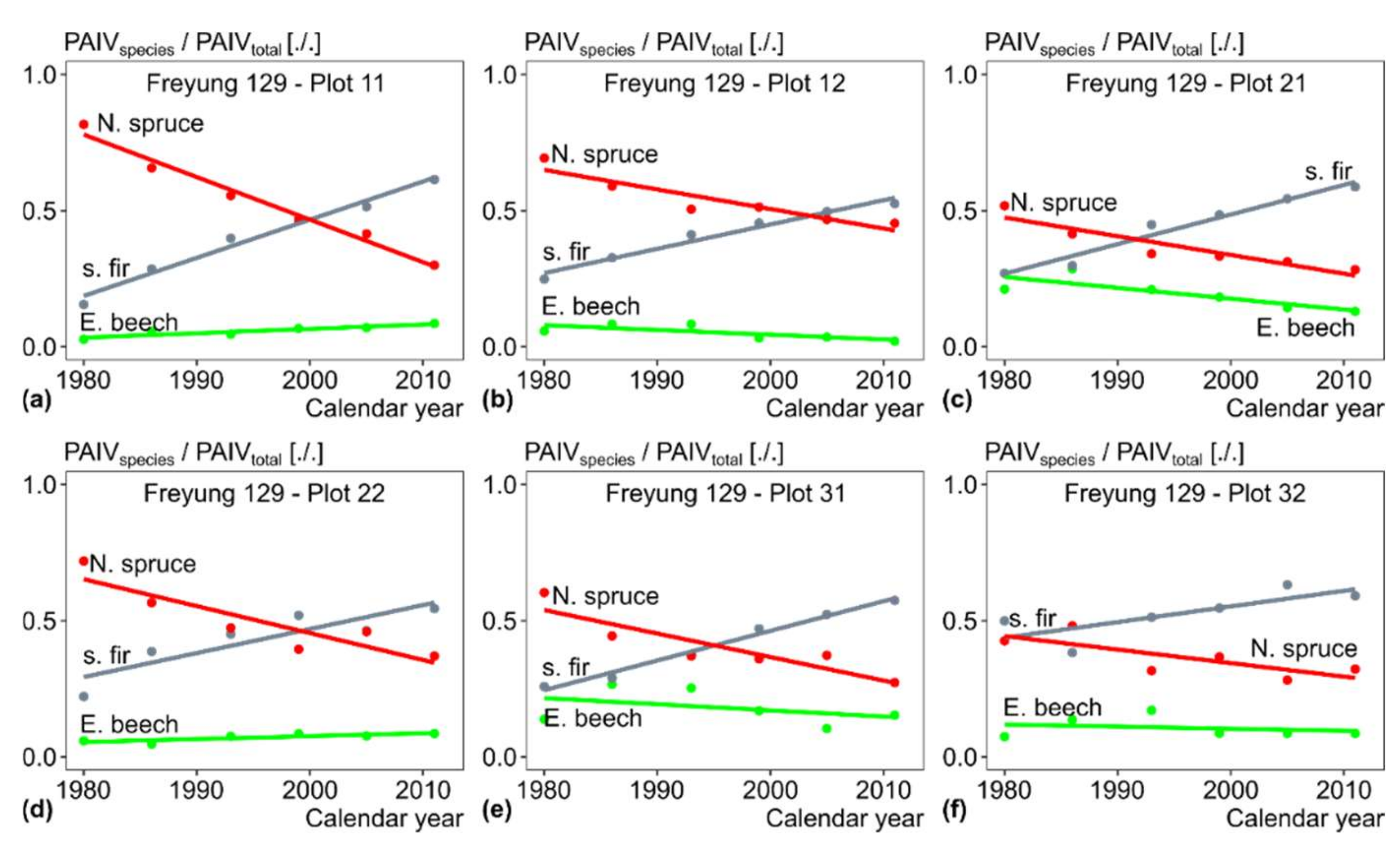
2.3.2. Species Level Evaluation

At the species level, we calculated the shares of the three tree species N. spruce, s. fir, and E. beech of the total periodic annual volume increment (PAIV). We calculated the respective shares by dividing the PAIV of a species by the total PAIV of all tree species taken together ($PAI{V}_{species}/PAI{V}_{total}$). We made these calculations for all six subplots and each observation period.

2.3.3. Diameter Distribution Level

For the exploration and modeling of the size-dependent distribution of the periodic annual stem volume growth, we used 10-cm diameter classes. We calculated the distribution for each subplot and survey period (see exemplarily Figures S4–S6). For further statistical analysis of the stem volume growth—diameter class distributions, we used the respective mean diameter of each DBH-class (e.g., 5 cm DBH in DBH-class 0–10 cm). To model the distribution and its temporal development, we fitted the distributions with generalized additive models (GAM) [61] separately for the three tree species N. spruce, s. fir, and E. beech and also the distribution for all species together. By this analysis, we revealed any change in the growth distribution, deviations from the steady state and compensation of one tree species by the other in term of their contribution to the stand structure and growth. Here, we focused on the subplots FRY 129/22, 129/31, and 129/32 which were kept at higher stand densities from 1980 to 2018 and faced only moderate density fluctuations in course of the periodic selection cuts to avoid cofounding effects of thinning on single tree growth. Since beech only played a minor role in the plots, it was of particular interest to investigate whether there occurred shifts in the contribution of the two species N. spruce and s. fir to the volume growth in the respective diameter classes. We investigated possible shifts using the relative periodic volume increment (RPAIV) per diameter class. This is the modeled periodic annual volume increment (PAIV) of the stronger species divided by the PAIV of the weaker species in each diameter class minus one; $RPAIV=PAI{V}_{stronger species}/PAI{V}_{weaker species}-1$). In the case that N. spruce was the stronger of the two species in a diameter class, we also multiplied the corresponding relative PAIV by minus one.

2.3.4. Tree Level Evaluation

Tree height estimation: For estimating the species-specific height, h, of each tree depending on the stem diameter, d, we parameterized the allometric relationship:

$$\ln \left(h\right)=a_0+a_1\times \ln \left(d_{ik}\right)+b_i+{\mathsf{\epsilon }}_{ik}$$

(1)

The assessment was based on n = 2919, 2360, and 1216 combined h- and d- measurements of N. spruce, s. fir, and E. beech between 1980 and 2018. The measurements were distributed over the whole diameter range. The model fitting resulted in the parameters $a_0=0.31$ and $a_1=0.80$ for N. spruce, $a_0=0.16$ and $a_1=0.86$ for s. fir, and $a_0=0.96$ and $a_1=0.62$ for E. beech with $R^2$ values of 0.95, 0.93, and 0.85, respectively (Supplementary Table S1). The individual tree heights predicted by this model were used as basis for the delimitation of the following neighborhood analysis.

Edge correction: Before calculating single tree-specific local competition values and mixing proportions for neighborhood analysis, we established a toroidal shift of the plot to all eight directions of the plot periphery for edge bias compensation [59,62,63]. Using the toroidal shift, we extended the same plant position pattern and distances in all eight directions and avoided any overestimation of density, as it could result from other techniques [63].

Neighborhood analyses within sample circles: To characterize the individual trees’ competitive status, we quantified the local stand basal area (BAL). For this purpose, we defined an influence zone by a circle with search radius $s{r}_1=0.25\times h_1$ around the position of each tree. All trees within the circle except the center tree were used to calculate the local basal area (ba) on the circle area a. $BAL=ba/a$ was the respective basal area upscaled to one hectare. In the constructed circles, there were, on average, 20–30 trees and at least 10–15 most impactful neighbors [64]. The BAL values were calculated with and without the removed trees ($BA{L}_{pre}$, $BA{L}_{post}$); based on both values, we quantified the competition release by the tree removal: $\Delta BAL=BA{L}_{pre}-BA{L}_{post}$.

Mixing proportions: The trees sampled in the circle were also used to calculate local mixing proportions. The mixing proportions $mportio{n}_1\dots mportio{n}_n$ should reflect the proportions of two or more species in the observed mixed stands [65,66]. Tree number, basal area, or volume proportions are only appropriate for this purpose if the mixed species have similar growing area requirements [67]. The considered tree species vary per se in the growing area requirement and maximum stand density in fully stocked stands. For example, a E. beech with a stem diameter of 25 cm may require approximately double the growing space as a N. spruce of the same diameter. This means the density in terms of trees per hectare is only half of that of N. spruce. To standardize the density and to calculate the unbiased area-related mixing proportions, we applied the equivalence factors according to [68]. These factors for the main tree species assemblages are shown in Supplementary Table S2.

Soil moisture Index (SMI): The Soil Moisture Index (SMI) is an indicator to quantify agricultural droughts. The SMI is simulated by the hydrologic model mHM using current weather data. The model mHM consists of a digital elevation model, geological map, soil map, and land cover and leaf area information derived from satellite data (see [69] for further explanation of the model). The model provides 30-day soil moisture indices SMI [70,71]. The range of the values is SMI = 0–1. A value SMI < 0.2 is considered as drought. The index is primarily used to provide information on the current moisture status of the soil. Applied mainly in climate research, the index is used for national drought monitoring in Germany [69]. Furthermore, the SMI has been successfully related to tree-ring series in dendroecological studies to identify drought events [72].

2.4. Statistical Models

For testing the overall growth trend of the stands (H I) we fitted the models:

$$\ln \left(IV\right)=a_0+a_1\times \ln \left(V_{ik}\right)+a_2\times \ln \left(V_{remove}{}_{ik}\right)+b_i+{\mathsf{\epsilon }}_{ik}$$

(2)

$$\ln \left(IV\right)=a_0+a_1\times \ln \left(V_{ik}\right)+a_2\times \ln \left(yea{r}_i\right)+a_3\times \ln \left(SM{I}_i\right)+b_i+{\mathsf{\epsilon }}_{ik}$$

(3)

in order to reveal any changes of IV by the volume of the removal trees, $V_{remove}$, or the calendar year.

Whether the long-term growth trend at the individual tree level has changed over time (H III) was tested by fitting the model:

$$\ln \left(id\right)=a_0+a_1\times \ln \left(d_{ik}\right)+a_2\times \ln \left(yea{r}_i\right)+a_3\times \ln \left(d_{ik}\right)\times \ln \left(yea{r}_i\right)+b_i+{\mathsf{\epsilon }}_{ik}$$

(4)

For the revelation of the causes of the long-term effects (H IV) we fitted the model:

$$\begin{array}{c}\ln \left(id\right)=a_0+a_1\times \ln \left(d_{ik}\right)+a_2\times \ln \left(BA{L}_{ik}\right)+a_3\times \ln \left(\Delta BA{L}_{ik}\right)+a_4\times \\ \ln \left(yea{r}_i\right)+a_5\times \ln \left(SM{I}_i\right)+a_6\times \ln \left(yea{r}_i\right)\times \ln \left(SM{I}_i\right)+b_i+{\mathsf{\epsilon }}_{ik}\end{array}$$

(5)

Another model was fitted to relate growth and driving variables of growth for the periods 1980–1993 (Model 6a) as well as 1993–2018 (Model 6b) in order to reveal any changes in the species-specific reaction patterns in the first compared to the second half of the survey period.

$$\begin{array}{c}\ln \left(id\right)=a_0+a_1\times \ln \left(d\right)+a_2\times \ln \left(BAL\right)+a_3\times \ln \left(\Delta BAL\right)+a_4\\ \hspace{1em}\hspace{1em}\hspace{1em}\hspace{1em} \times \ln \left(mportion\right)+a_5\times \ln \left(SMI\right)+b_i+{\mathsf{\epsilon }}_{ik}\end{array}$$

(6)

Model 6 reveals the effects for the first and second half of the survey period how the stress effect modified the growth of the three species and how selection cutting were able to modify the environmental impact (H V).

For testing H I, H III, H IV, and H V, we applied linear mixed models. The dependent variables were either the stand stem volume growth, IV (Models 2 and 3), or the mean annual stem diameter growth, id (Models 4–6). The independent variables were in the case of Models 2 and 3 the standing stem volume, V, the volume of the removal trees, $V_{remove}$, the soil moisture index, SMI, and the calendar year, year. In the case of Models 4–6, the independent variables were the individual tree diameter, d, local basal area, BAL, release by tree removal, $\Delta BAL$, mixing proportion, mportion, soil moisture index, SMI, and the calendar year, year. In all equations, the indexes i and k represent the k^th observation of the i^th plot (Models 2 and 3) or tree (Models 4–6). The fixed effects were covered by the parameters $a_0$–$a_n$. With the random effect $b_i~N\left(0,{\tau }^2\right),$ we cover the correlation between the single observations on plot (Models 2 and 3) and tree (Models 4–6) level. In preliminary model formulations of the Models 4–6, we also worked with random effects on plot level, i.e., one additional nesting level. As this caused confounding effects with the fixed effect, we constrained ourselves to the simpler random effect structure of Equations (3)–(6). With ${\epsilon }_{ik}$, we denote the independently and identically distributed errors.

Hypothesis H II, whether the overall growth distribution on the trees in different diameter classes was modified over the entire survey period 1980–2018 was tested by fitting a generalized additive model (GAM) to the data of the subplots FRY 129/22, 31, and 32.

$$PAI{V}_{DBHclass}=period+s\left(DB{H}_{class mean}\right)+s\left(DB{H}_{class mean},by=period\right)$$

(7)

Here, we analyzed any growth change in the respective DBH-classes of the distribution over time (period = single observation period); no significant differences between the observation periods would indicate a steady state. Any deviation between observation periods in each DBH-class would indicate temporal changes.

For assessing whether there were changes in the PAIV within the DBH-classes between the species, we first fitted a generalized additive model for each observation period individually.

$$PAI{V}_{DBHclass}=Species+s\left(DB{H}_{class mean}\right)+s\left(DB{H}_{class mean},by=Species\right)$$

(8)

Using this model, we were able to derive the corresponding relative annual periodic volume increments (RPAIV) in the 10 cm diameter classes (see Section 2.3). To test whether there were temporal changes in the RPAIV values in the respective diameter classes, we used another generalized additive model for the plots Freyung 129/22, 31, and 32.

$$RPAI{V}_{DBHclass}=s\left(DB{H}_{class mean}\right)+s\left(period\right)+s\left(DB{H}_{class mean},period\right)$$

(9)

We restricted evaluation for testing HII and HIII on data of the subplots FRY129/22, 31, and 32 where the standing volume was kept continuously at a high level since the beginning of the survey. In this way, we could eliminate silvicultural effects on growth dynamic and elucidate environmentally triggered changes.

All data processing including the toroidal shifts and analyses were conducted using the statistical software R version 4.0.5 [73], specifically employing the packages tidyverse [74], nlme [75], lme4 [76], and mgcv [61].

3. Results

3.1. Tree and Stand Characteristics

The dendrometric stand characteristics (

Table 2. Overview of key stand characteristics of the selection forest experimental plot FRY 129. The table reflects the mean, standard deviation, minimum and maximum values of the 6 subplots FRY 129/11, 12, 21, 22, 31, and 32 at the last survey in 2018. The reported mean periodical growth rates refer to the period 2011–2018.

Variable	Unit	Mean	Sd. Dev.	Min	Max
Tree number	ha−1	848.67	160.55	688.00	1080.00
Mean height	m	19.59	1.44	17.40	21.22
Mean diameter	cm	25.24	3.01	21.46	28.87
Stand basal area	m2 ha−1	42.48	10.84	29.11	59.87
Standing volume	m3 ha−1	610.63	188.05	373.57	873.11
Volume proportion N. spruce	./.	0.45	0.08	0.35	0.56
Volume proportion s. fir	./.	0.46	0.05	0.41	0.53
Volume proportion E. beech	./.	0.09	0.05	0.01	0.17
Basal area growth	m2 ha−1 yr−1	0.80	0.09	0.68	0.90
Stem volume growth	m3 ha−1 yr−1	12.40	1.88	10.04	15.59

) show that the tree sizes are quite similar on the different plots (e.g., mean stem diameter 21.46–28.87 cm) but the stand density differs strongly. As a result of the silvicultural density regulation, the tree number, basal area, or standing volume of plots with high density show doubled values compared to the most sparsely stocked plot (e.g., 373.57 vs. 873.11 m³ ha⁻¹). However, the volume growth differs less strongly (10.04 vs. 15.59 m³ ha⁻¹ yr⁻¹). The mean volume proportions corrected by mixing portion are similar for the conifers (0.45 and 0.46, respectively). It varies most pronounced (0.35–0.56) in case of N. spruce and the lowest in case of s. fir (0.41–0.53). Due to the lack of printing space, we restrict the introduction of the experimental stands to the information essential for understanding this study. For details of the stand structure, overstorey growth, and regeneration, see [9,17,48,49].

Typically, for selection forests, the trees on the plots belong to very different age phases and social positions.

Table 3. Overview of the main data (comprising inventories from 1980 to 2018) for analyzing the dependency of the annual stem diameter growth, id, on stem diameter, d, crown diameter, cd, height, crown length, crown ratio, h/d-ratio, local stand density index, BAL, mixing proportion of the second species, mportion. Species-specific sample sizes, n, mean, standard deviation, minimum and maximum values for the three analyzed species combination are shown.

Variable	Unit	Mean	Sd. Dev.	Min	Max
N. spruce, n = 2919
id	cm yr−1	0.39	0.23	0.02	1.15
d	cm	38.94	25.10	7.00	89.50
cd	m	5.50	2.03	2.27	12.32
height	m	24.09	12.67	4.20	42.80
crown length	m	14.77	8.24	2.00	31.40
crown ratio	m m−1	0.61	0.10	0.23	0.90
h/d-ratio	m cm−1	0.69	0.15	0.42	1.12
BALpre	m2 ha−1	40.00	33.27	0.52	196.68
BALpost	m2 ha−1	37.14	31.97	0.52	196.68
ΔBAL	m2 ha−1	2.87	10.85	0.00	187.45
mportion	./.	0.50	0.34	0.00	1.00
s. fir, n = 2360
id	cm yr−1	0.17	0.15	0.01	0.73
d	cm	21.55	14.59	7.00	91.00
cd	m	4.94	1.52	1.65	9.88
height	m	16.27	8.98	4.80	41.40
crown length	m	9.16	6.09	1.10	28.40
crown ratio	m m−1	0.54	0.15	0.16	0.87
h/d-ratio	m cm−1	0.78	0.12	0.45	1.12
BALpre	m2 ha−1	50.46	27.10	0.48	199.23
BALpost	m2 ha−1	45.63	26.52	0.47	199.23
ΔBAL	m2 ha−1	4.82	11.38	0.00	122.30
mportion	./.	0.56	0.30	0.00	1.00
E. beech, n = 1216
id	cm yr−1	0.27	0.15	0.01	0.70
d	cm	33.44	14.81	7.50	70.00
cd	m	9.53	2.35	4.00	16.18
height	m	21.85	6.53	5.10	34.80
crown length	m	16.22	4.96	2.50	24.90
crown ratio	m m−1	0.75	0.11	0.49	0.92
h/d-ratio	m cm−1	0.71	0.20	0.24	1.24
BALpre	m2 ha−1	47.44	32.51	0.69	184.90
BALpost	m2 ha−1	44.78	31.67	0.69	184.41
ΔBAL	m2 ha−1	2.66	9.34	0.00	119.15
mportion	./.	0.75	0.27	0.00	1.00

reflects the wide range of tree state variables and stem diameter increment represented on the six plots. The tallest trees achieve 89.5 cm stem diameter, 42.8 m tree height, 31.40 m crown length, and 16.18 m crown diameter. E. beech has on average lower tree heights but wider lateral crown expansion, longer crowns, and higher crown ratios. Altogether, more than 6000 stem records from the repeated surveys and their variation in size and tree development and competitive state provide a solid database for the subsequent evaluation of the tree growth depending on tree status, competition, and environment.

The mean local densities before and after thinning, BAL_pre and BAL_post, respectively, are higher for the highly shade tolerant s. fir and E. beech compared with N. spruce, whereas the minimum and maximum values are similar for all species. The release by selection cutting, $\Delta BAL$, was the highest for s. fir. The mean proportion of other species in the neighborhood, mportion was 0.50, 0.56, 0.75 for N. spruce, s. fir, and E. beech; this reflects that the stands were dominated by the two conifers.

The mean stem diameter growth plotted over the calendar year revealed a clear species-specific trend (Figure 3a–c). Obviously, N. spruce decreased in growth since the start of the survey in 1980; in the middle of the survey period, the decrease was nearly linearly, during the last 20 years, the decrease lessened. S. fir, in contrast, continuously increased in growth since 1980; the mean growth rate more than doubled. E. beech showed a unimodal course of growth with a peak in the 1990s when growth of N. spruce was already reduced and s. fir not yet reached the maximum.

Additionally, to the course of the mean stem diameter growth depending on calendar year (Figure 3), the Supplement Figures S1–S3 show the growth of all individual trees versus calendar year and the growth plotted over stem diameter. The shown species-specific growth trends may be co-determined by the stand structure and silvicultural treatment of the plots. To avoid respective biases, we considered those effects in the following analyses.

3.2. Development of Stand Level Growth (H I)

Figure 4a shows that the stem volume growth on the plots FRY 129/11-32 ran on different levels and varied, but remained on a rather constant level of about 10–15 m³ ha⁻¹ yr⁻¹ since 1980. There was a tendency that the plots with the higher standing volume at the beginning of the respective survey periods had higher productivity than the plots with lower stand volume (Figure 4b).

We further analyzed the dependency of stand stem volume growth on volume and removed volume by selection cuttings (Figure 4c,

Table 4. Statistical characteristics of the Models 2–6. The model numbers refer to Section 2.4 where the models are introduced in detail. For reasons of space, the table reports just the fixed effect variables of the respective models (Part one).

Model	Species	n	${\mathit{a}}_0$	Std $\left({\mathit{a}}_0\right)$	p-Value	${\mathit{a}}_1$	Std $\left({\mathit{a}}_1\right)$	p-Value	${\mathit{a}}_2$	Std $\left({\mathit{a}}_2\right)$	p-Value	${\mathit{a}}_3$	Std $\left({\mathit{a}}_3\right)$	p-Value	${\mathit{a}}_4$	Std $\left({\mathit{a}}_4\right)$	p-Value	${\mathit{a}}_5$	Std $\left({\mathit{a}}_5\right)$	p-Value	${\mathit{a}}_6$	Std $\left({\mathit{a}}_6\right)$	p-Value
2	all species	216	0.44	0.53	0.405	0.29	0.08	<0.001	0.04	0.01	<0.001
3	all species	216	3.19	16.15	0.843	−0.13	0.08	0.134	0.01	2.12	1.00	0.01	0.15	1.00
4	N. spruce	276	1351.66	281.99	<0.001	−259.19	74.82	0.009	−178.24	37.09	<0.001	34.17	9.84	<0.001
4	s. fir	382	−1068.54	278.95	<0.001	207.60	79.75	<0.001	140.24	36.72	<0.001	27.26	10.50	0.009
4	E. beech	179	1202.78	455.42	0.009	−325.06	136.49	0.018	−158.50	59.90	0.008	42.78	17.95	0.018
5	N. spruce	675	144.31	43.69	<0.001	0.60	0.04	<0.001	−0.09	0.05	0.073	0.10	0.03	<0.001	−19.35	5.76	<0.001	0.69	0.37	0.063
5	s. fir	893	3828.77	1870.84	<0.041	0.65	0.04	<0.001	−0.25	0.05	<0.001	0.13	0.02	<0.001	−503.69	246.03	<0.040	6489.43	2819.47	<0.022	−853.17	370.75	<0.021
5	E. beech	285	−1.44	0.47	0.003	0.30	0.06	<0.001	−0.14	0.09	<0.001	0.16	0.04	0.100				1.04	0.51	0.042
6a	N. spruce	246	−2.54	0.43	<0.001	0.55	0.07	<0.001	−0.22	0.11	0.042				0.76	0.27	0.005
6a	s. fir	421	3.90	1.97	0.049	0.80	0.07	<0.001	−0.28	0.08	0.001	0.17	0.04	<0.001				11.55	3.02	<0.001
6a	E. beech	89	−4.13	0.62	<0.001	0.23	0.17	0.184				0.13	0.06	<0.001	2.95	0.52	<0.001
6b	N. spruce	435	−2.72	0.33	<0.001	0.67	0.05	<0.001	−0.08	0.07	0.201	0.17	0.04	<0.001
6b	s. fir	494	−2.37	0.30	<0.001	0.55	0.05	<0.001	−0.22	0.07	0.002	0.12	0.03	<0.001				1.20	0.37	0.002
6b	E. beech	194	−1.25	0.48	0.009	0.27	0.07	<0.001	−0.12	0.09	0.188	0.22	0.05	<0.001	0.39	0.16	0.014

Model 2: $\ln \left(IV\right)=a_0+a_1\times \ln \left(V_{ik}\right)+a_2\times \ln \left(V_{remove}{}_{ik}\right)+b_i+{\mathsf{\epsilon }}_{ik}$; Model 3: $\ln \left(IV\right)=a_0+a_1\times \ln \left(V_{ik}\right)+a_2\times \ln \left(yea{r}_i\right)+a_3\times \ln \left(SM{I}_i\right)+b_i+{\mathsf{\epsilon }}_{ik}$; Model 4: $\ln \left(id\right)=a_0+a_1\times \ln \left(d_{ik}\right)+a_2\times \ln \left(yea{r}_i\right)+a_3\times \ln \left(d_{ik}\right)\times \ln \left(yea{r}_i\right)+b_i+{\mathsf{\epsilon }}_{ik}$; Model 5: $\ln \left(id\right)=a_0+a_1\times \ln \left(d_{ik}\right)+a_2\times \ln \left(BA{L}_{ik}\right)+a_3\times \ln \left(\Delta BA{L}_{ik}\right)+a_4\times \ln \left(yea{r}_i\right)+a_5\times \ln \left(SM{I}_i\right)+a_6\times \ln \left(yea{r}_i\right)\times \ln \left(SM{I}_i\right)+b_i+{\mathsf{\epsilon }}_{ik}$; Model 6: $\ln \left(id\right)=a_0+a_1\times \ln \left(d\right)+a_2\times \ln \left(BAL\right)+a_3\times \ln \left(\Delta BAL\right)+a_4\times \ln \left(mportion\right)+a_5\times \ln \left(SMI\right)+b_i+{\mathsf{\epsilon }}_{ik}$.

Model 2). Stem volume growth slightly decreased with lower stand densities; the model coefficient $a_1$ indicates that a density reduction of the volume by 50% reduced the productivity only by ~30%. This indicates a subproportional effect of density reduction on stand growth; in case of a proportional effect, $a_1$ would equal 1. The removal stand volume at the beginning of the survey period increased the volume growth. Especially moderate selection cutting by removal of 50–100 m³ ha⁻¹ increased the productivity, whereas stronger density reductions had only minor additional effects (saturation curve).

Neither the calendar year nor the soil moisture index had a significant effect on the stand volume production (Figure 4d); indicated by slopes of zero in the regression of stem volume versus calendar year and SMI (Table 4, Model 3).

Our results about the shares of the three tree species N. spruce, s. fir, and E. beech in the total volume growth showed that they have changed substantially since the beginning of the experiment in 1980 (Figure 5). The share of s. fir concerning volume growth has steadily increased in all subplots. The proportion of N. spruce has decreased to almost the same extent as the proportion of s. fir has increased. E. beech, on the other hand, has remained almost constant in its share of volume growth. Although the shares in volume growth on the subplots FRY 129/11, 12, and 21 were more strongly co-determined by selection cuttings, it is of special interest that we found this pattern also on the moderately thinned and highly stocked subplots FRY 129/22, 31, and 32.

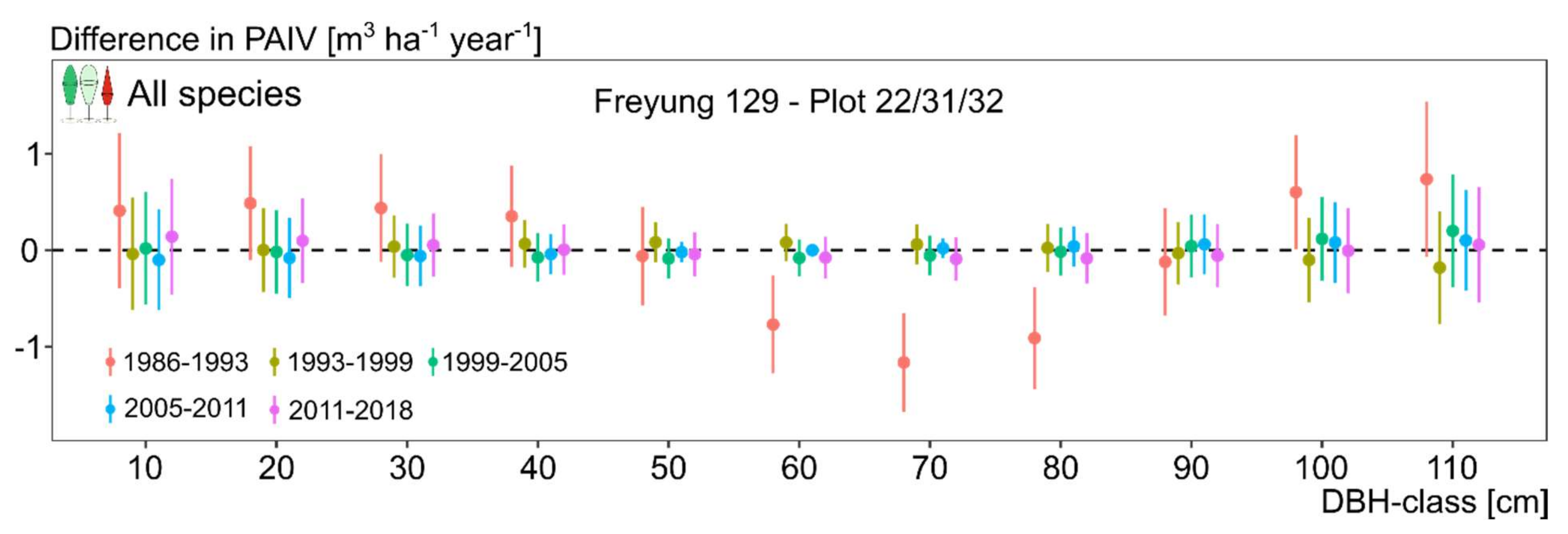
3.3. Size Class Contribution to Stand Growth over Time (H II)

By fitting Model 7 to the total volume growth distributions (m³ ha⁻¹ year⁻¹ for DBH-classes) of all tree species together on the subplots FRY 129/22, 31, and 32, we found a significant deviation of the distribution only for the first observation period 1980–1986 (

Table 5. Results of fitting the generalized additive model from Equation (7) to the data of the subplots FRY 129/22, 31, and 32. Period 1986 refers to the growing period from 1986 to 1992 and so on.

Fixed Effect Variable	t Value	p Value
Intercept	10.601	<0.001
period 1986	−1.905	0.058
period 1993	−0.244	0.807
period 1999	−0.623	0.534
period 2005	−0.699	0.485
period 2011	−0.707	0.481
Smooth terms	F value	p value
DBH-class	13.649	<0.001
DBH-class: period 1980	4.335	<0.001
DBH-class: period 1986	0.041	0.851
DBH-class: period 1993	0.526	0.665
DBH-class: period 1999	0.019	0.898
DBH-class: period 2005	0.036	0.860
DBH-class: period 2011	0.219	0.788

, Figure 6) in the 50–60 cm, 60–70 cm, and 80–90 cm diameter classes (the confidence interval excludes zero). Since 1986, the total volume growth distribution has not shifted significantly on these plots (Figure 6). From 1986 to 2018, we could not detect any significant changes in any of the 11 diameter classes.

If all three tree species are considered together, the volume increment distributions on the fully stocked subplots FRY 129/22, 31, and 32 are almost constant since 1986 (Figure 6). Figure 5 showed, however, that the shares of the two tree species N. spruce and s. fir in the total PAIV have changed substantially even after 1986.

It was of particular interest to see in which diameter classes this shift has taken place. Our results from Model 9 (

Table 6. Results of fitting the generalized additive model from Equation (9) to the data of the subplots FRY 129/22, 31, and 32.

Fixed Effect Variable	t Value	p Value
Intercept	4.631	<0.001
Smoother terms	F value	p value
DBH-class	0.772	0.492
period	2.966	0.034
DBH-class, period	0.786	0.001

) showed on the one hand that there was a significant temporal change in the relative PAIV between N. spruce and s. fir, but they also provide information on the diameter classes in which these shifts took place (Figure 7). S. fir had at any time higher RPAIV in smaller diameter classes (10–50 cm DBH). In the diameter classes 50–60, 60–70, and 70–80 cm DBH, we observed a change in growth dominance between the two species N. spruce and s. fir. In the first surveys, N. spruce still had a higher share of growth in these diameter classes. However, during the last surveys, it was s. fir that showed a higher share of growth in the respective diameter classes. N. spruce had at any time higher RPAIV in higher diameter classes (80–110 cm DBH). However, it is remarkable that the growth dominance of spruce in these diameter classes has declined substantially since 1980. In the 110–120 cm diameter class, the situation was almost balanced between the two species.

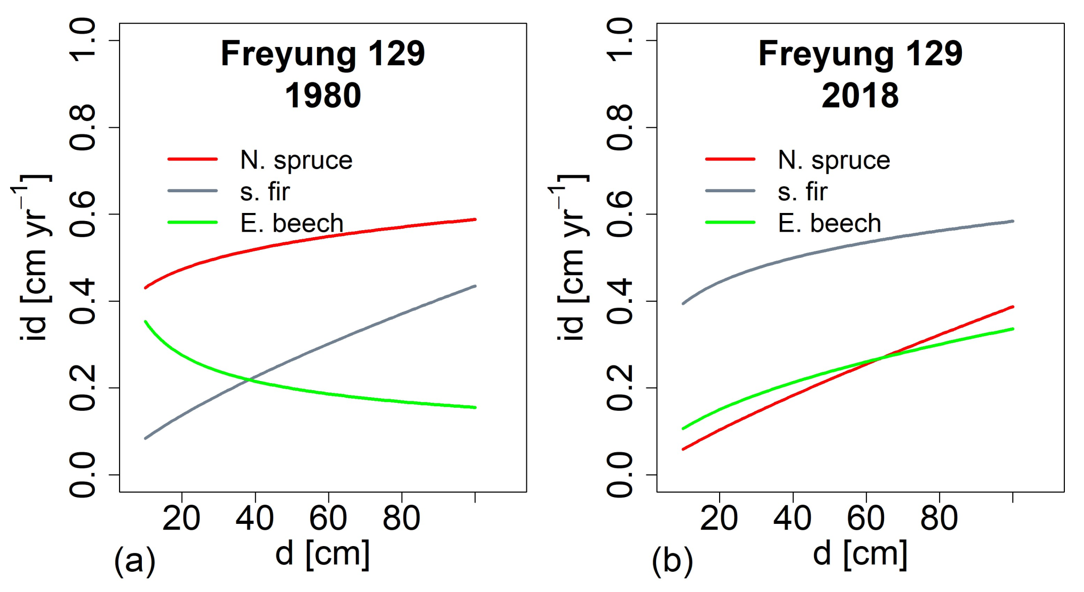
3.4. Change of Growth and Growth Partitioning from 1980ies to Present (H III)

The visual comparison between the growth-size relationship of the three species (Figure 8a,b) shows a fundament change of the species ranking from the first survey in 1980 to the last in 2018. Under constant environmental conditions and steady state, structure and volume on the plots the species-specific level and slope of the id-d relationship should be similar in 2018 compared to 1980. However, s. fir was inferior to N. spruce in the past and shows superior growth at present. E. beech also improved in growth, but to a lower extent than s. fir. For N. spruce, applies the opposite; it was superior in the past and decreased in the id-d relationship.

In addition to the visual comparison, Model 4 revealed that the growth changed significantly depending on the calendar year within the survey period from 1980–2018. For N. spruce and E. beech, the stem diameter growth decreased since 1980 (see Model 4 in Table 4, a₂ = −178.24 and a₂ = −158.50, respectively). For s. fir, the regression coefficient in Table 4 reveals a significant increase of the level (a₂ = 140.24) of the stem diameter growth relationship. Both N. spruce and E. beech show a decrease of the level and increase of the slope of the id-d relationship on the high density plots from 1980–2018. As we used only data from subplots less affected by selective cuttings, we identify environmental changes responsible for the role reversal in favor of s. fir within the last 40 years.

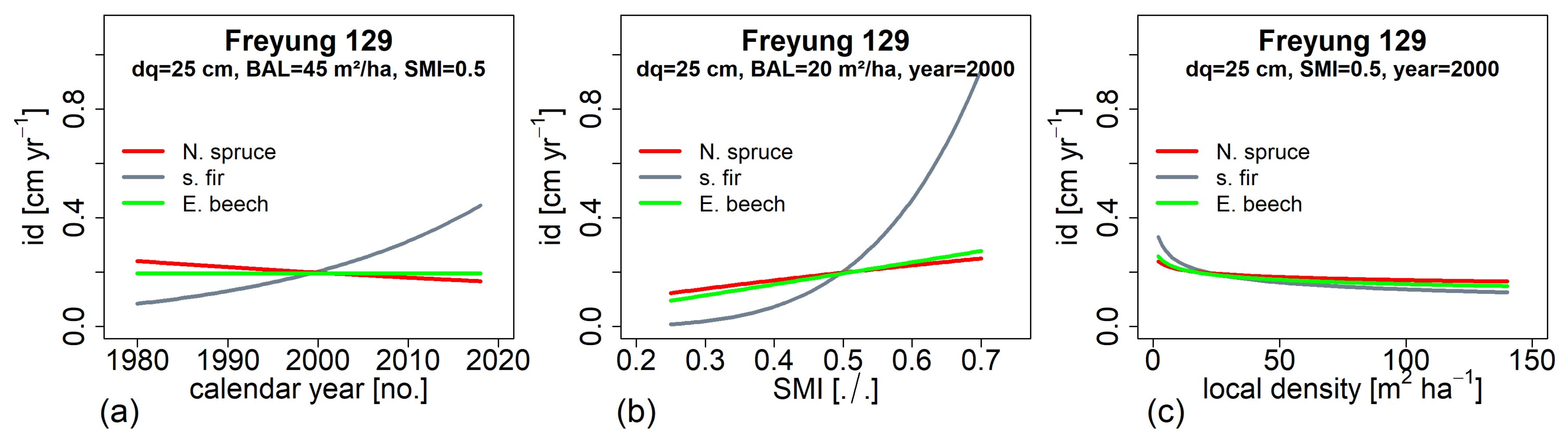
3.5. Impact of Environmental Factors on Growth Development (H IV)

S. fir continuously improved in stem diameter growth since 1980 according to the evaluation by Model 5 (Figure 9a). Note that we modified the calendar year, but set the other model variables constant to show this significant trend. N. spruce decreased significantly, and E. beech showed no trend between 1980–2018. Thus, the ranking between the species in terms of growth changed from initial N. spruce > E. beech > s. fir to the opposite at the end of the survey period. At parity of diameter, local stand density, and SMI stem growth of silver was more than threefold in 2018 compared with 1980.

All three species react positively to SMI, however, s. fir much stronger than N. spruce and E. beech (Figure 9b). In dry years, s. fir reduced growth stronger than N. spruce and E. beech, but benefitted most from improving water availability.

The growth of all three species depended similarly on the local stand density (Figure 9c). Stem diameter growth decreased continuously with increasing local stand density BAL. This reaction pattern was shown for the year 2000, SMI conditions of 0.5, and trees with mean diameter of d = 25 cm, however, the relationship between the species changed with the SMI conditions.

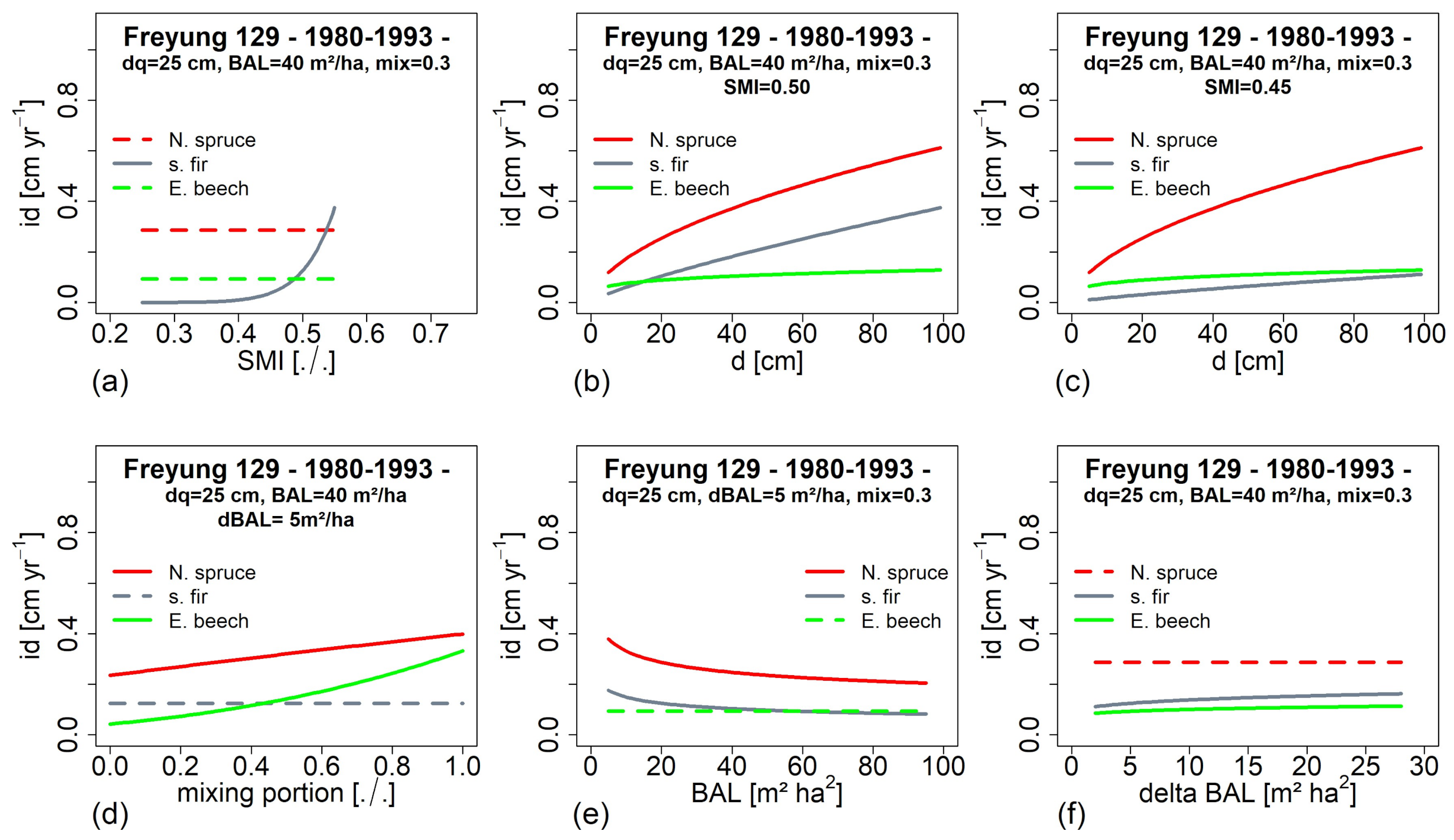
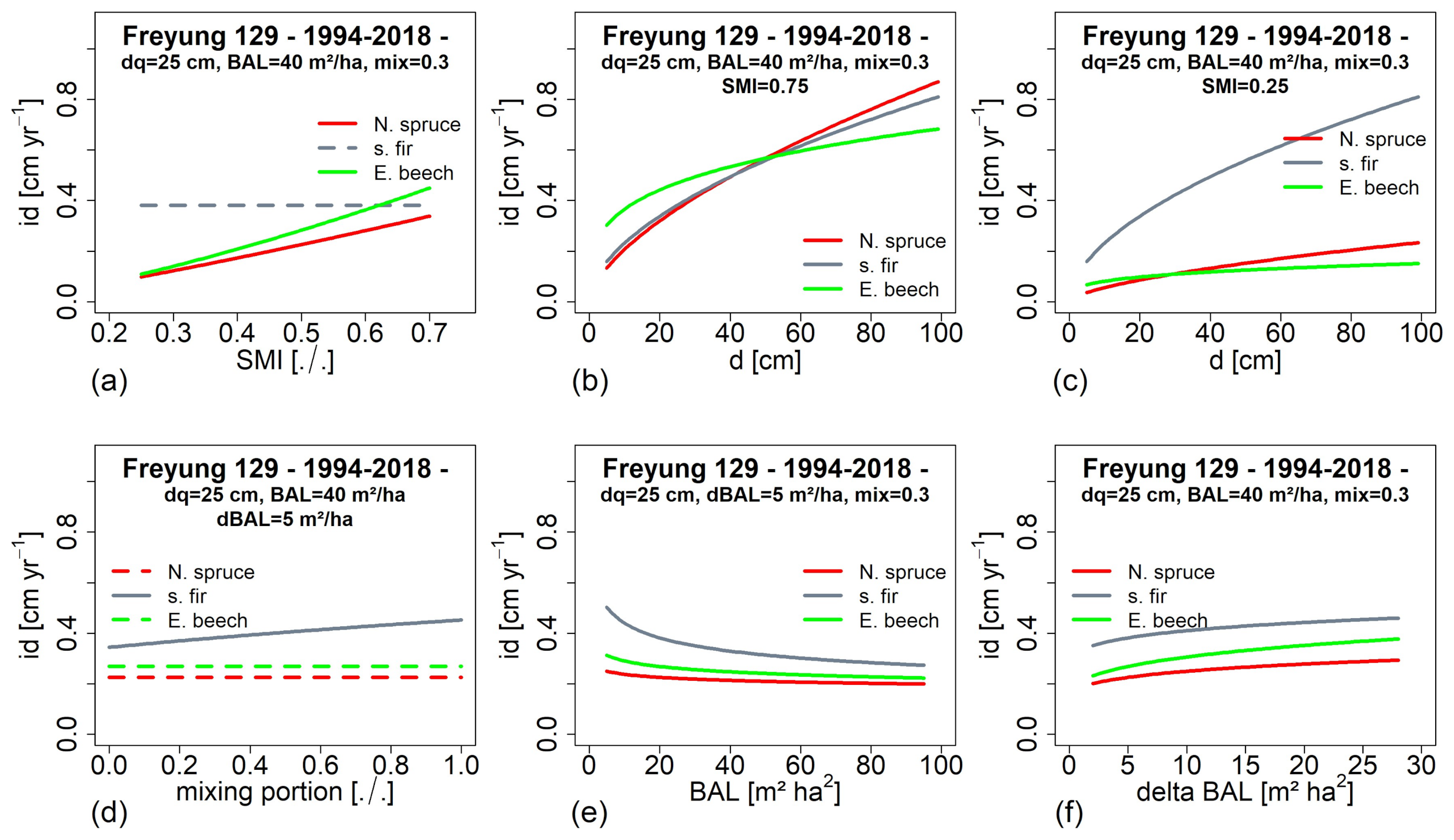
3.6. Tree Growth Depending on Environemnatl Conditions in the Past and at Present (H V)

In the period 1980–1993 when the atmospheric SO₂-load was high, we found a high sensitivity of silver to drought, indicated by a strong reduction of stem diameter growth with decreasing SMI (Figure 10a). For N. spruce and E. beech, we found no dependency of growth on SMI (broken lines). This caused a strong decrease of the relationship between id and d of s. fir even by a moderate reduction from SMI = 0.50 to SMI = 0.45 (Figure 10b,c). In the period 1980–1993, different tree species in the neighborhood were beneficial for N. spruce and E. beech, but not for s. fir (Figure 10d). Density reduction slightly increased the stem diameter growth of N. spruce and s. fir but not the growth of E. beech (Figure 10e). Selection interventions had a slightly positive effect on the growth of s. fir and E. beech, whereas N. spruce reacted independently from the intervention intensity (Figure 10f).

In the period with low atmospheric SO₂-load (1994–2018), s. fir grew rather independent from SMI, whereas N. spruce and E. beech reduced their growth significantly under drought. The growth stability of s. fir under drought may partly result from the reduced water consumption by the neighboring species (Figure 11a). In wet years, N. spruce is superior in growth (Figure 11b), however, under drought, s. fir turns the best and N. spruce and beech strongly reduce their stem growth. The slight increase of fir in dry years may result from a competition reduction due to the more drought affected neighboring N. spruces and beeches (Figure 11c). This is in line with the finding that silver benefits from species admixture in the neighborhood, whereas N. spruce and E. beech hardly react on increasing mixing proportion in the vicinity (Figure 11d). S. fir show the highest growth rates over the whole range of local stand densities (Figure 11e) and also reacts most strongly on a given density release by selection cutting (Figure 11f).

4. Discussion

4.1. Individual Tree Resilience versus Stand Level Resilience

In contrast to the species-specific reaction patterns of individual tree growth, stand productivity remained rather constant since 1980. In essence, stand productivity depended on density and structure regulation but hardly on environmental conditions. Obviously, the species-specific stress and growth reduction of one species was buffered by the increase of another resulting in a neutral net effect on stand productivity. Note, that an analysis at the individual tree level indicated a growth decrease for s. fir in 1980–1990 and for N. spruce in the 2010–2018. A deduction of stand growth based on the finding at the individual tree level would be misleading without considering the counteracting and counterbalancing effect between the tree species. Upscaling of growth reactions from tree level to stand level should be made cautiously; a diversity of species traits, stress susceptibility, growth compensation between different layers and asynchrony of stress reactions can buffer and neutralize growth patterns at the stand level that are alarming at the tree level. On the other hand, our analysis showed that findings of a constant productivity at the stand level may be misguiding; thus, we were able to show with our results that, if all tree species are considered together, the distribution of volume growth across the diameter classes has not changed since 1986. However, we were also able to show that the shares of the three tree species in volume growth in the respective diameter classes have shifted significantly over the last 40 years. Especially in the smaller and medium diameter classes, N. spruce showed a declining share. This declining share of N. spruce was compensated by the re-strengthening of s. fir, so that the volume growth distribution at the stand level remained constant. However, it also led to the fact that fir has become dominant in terms of standing stock and volume growth. These findings point out that despite constant accumulative growth, the contribution of different species and layers may change and thus the system structure may also change.

4.2. Diversity Promotes Stability

The recovery of s. fir after reduction of SO₂-emissions is a model example for the society’s capacity to advocate, decide, and act in favor of nature including forest ecosystems. Starting with the environmental political measures of industry emission reduction in the 1970s and 1980s focusing on SO₂-emissions of the coal electric power plants air pollution has been significantly reduced and simultaneously the far-distant transport of pollution to the low and high mountains among other to the Bavarian Forest [51,52]. This enabled especially the recovery of s. fir which is highly susceptible to damage caused by sulfur emissions [19].

In selection forests, particularly dominant s. firs had suffered from the emissions; subdominant und understory s. firs survived, could recover after emission reduction, and recaptured their key role for the sustainable productivity and functioning beside N. spruce and E. beech. The ability of s. fir to “sit and wait” and survive in subdominant position enabled its comeback after the strong decline due to acid rain.

In the 1980s, s. fir was on a low growth level in all diameter classes. In addition, it reacted very negatively on dry years. This means that the vitality reduction by SO₂ was linked with an increased drought sensitivity [51]. Evaluations of the crown vitality showed a high crown transparency due to needle losses in the 1980s and 1990s; this needle shedding probably caused a growth reduction, deeper irradiation into lower canopy layers, and maybe promoted N. spruce and E. beech which in return may have increased the competition for water disadvantageous for s. fir.

Maintaining tree species, even when vitality is reduced, may be advantageous in future times. Keeping and promoting s. fir in phases of strong emissions despite damages creating a potential for strong recovery soon afterwards. A further pro for the s. fir was its lower susceptibility to drought stress when other stress factors are absent. That became relevant in the second half of the survey period. Since the 1990s, s. fir not only stabilized stand growth by its recovery from emission damages but also by compensating the growth losses of N. spruce and E. beech caused by drought events, among others in the years 2003 and 2015.

4.3. Management of Diversity

The stable productivity within the study plots were so far based on their specific tree species diversity. In the 1980s, N. spruce had a share of 56% of the standing stock and 63% of the stand productivity, so that the growth losses of s. fir caused by SO₂ could be compensated by N. spruce. The other way round, the increasing drought stress of N. spruce since 2000 was compensated by the steadily recovering and more drought resistant s. fir. Due to its reviving vitality, s. fir became dominant in terms of standing stock and growth of volume, whereas N. spruce decreased. E. beech was kept on a rather low level, due to its inferior wood quality. The overrepresentation of s. fir and its essential contribution to the stand productivity is advantageous now, however, suppose it would be impaired by new biotic or abiotic disturbances the stands might strongly suffer due to this dominance. Anticipatory and preventive silvicultural management might balance the proportions of the three species or even increase the species diversity by adding stress resistant provenances of present species or even additional species such as Douglas-fir (Pseudotsuga menziesii) or yew tree (Taxus baccata), to ensure genetic or species diversity and to stabilize productivity according to the insurance theory [37]. The presently high productivity may be a misleading indicator for general productivity and system stability without considering how it is backed by tree species diversity. Maybe stand productivity divided by the tree species evenness would be a better indicator.

When stand density is reduced in selection forests, productivity eventually also decreases; however, the decrease starts off at much lower density and proceeds much slower than in even-aged monocultures. The reason for this broader saddle and lower steepness of the stand density-productivity relationship lies in the trees of the medium and lower layer, which can buffer and compensate the growth losses of the removal stand immediately [77]. The primarily tree-wise interventions and removals only cause small gaps, which can be closed quickly by trees of lower layers and by neighbors. The halving of the standing stock from 600 to 300 m³ ha⁻¹ on one subplot of the Freyung experimental resulted in a growth reduction of only 20–30% compared to the fully stocked stand (Figure 4c). It indicates a high growth resilience of the selection forest to silvicultural or natural disturbances compared with the age class forest. In the latter, any gaps in the canopy may be closed much slower due to the mono-layering and lack of natural regeneration.

The potential to mitigate impacts of stress situations on stand level growth by density management needs to take species-specific traits concerning stress susceptibility into account; our results show that the species-specific effect of density regulation very much depended on the prevailing stress factor.

4.4. Methodological Consideration

Compared to other competition indices, the local stand basal area BAL is easy to interpret and to link with practical decision making; stand basal area is a well known measure which is easy to assess e.g., by relascope sampling [78] and frequently used in silvicultural models and prescription [59,79]. The search radius of half of the tree height caused a size dependent delineation of neighborhood analyses as proposed by [80] and resulted in BAL and $\Delta BAL$ values that correlated closely ($R^2$ > 0.6) with the stem diameter growth. By application of density equivalence factors [65], we considered the species-specific growing space requirements when merging/summarizing the effect of different competitive strength of neighboring species in one index. Alternative indices, e.g., based on crown size or leaf area, would have required more detail survey data; BAL and $\Delta BAL$ used only stem diameter and height which were measured most frequently since the start of the survey.

4.5. Relevance for Climate Smart Forest Management

The concept of Climate Smart Forestry [81] aims at enhancing the adaptive and mitigative potential of forest in the frame of climate change, concurrently providing multiple benefits for society. The stable growth of the here investigated selection forest despite changing environments and associated disturbance patterns indicates a high level of resilience of the system. This level is achieved by mixing species of different traits and susceptibility to stress factors as well as by sustaining the specific forest structure. Applying the indicators of Climate Smart Forestry [81] to the specific plots resulted in generally high and stable over time smartness values [82] for selected indicators. Those selected indicators refer to the underlying criteria of sustainable forest management, global carbon cycle, health and vitality, productive function, and biological diversity [83]. In that sense, selection forestry seems to permit a high potential of adaptability and sustainable delivery of forest functions.

5. Conclusions

The successful reduction of ${\mathrm{SO}}_2$-emissions and recovery of tree growth and vitality demonstrate that human engagement in environmental policy can revive forest ecosystem health. Selection forests of N. spruce, s. fir, and E. beech that are common in the submontane to subalpine zone proved to be well adapted to environmental changes. Their combination of species diversity and structural heterogeneity can stabilize growth and promote climate smartness. The study object corroborates that uneven-aged, multi-layered mixed stands, which are the target stands of many present transitioning programs can result in rather stress resistant ecosystems and in stable productivity on the given sites. Next, steps should encompass analogous analyses regarding other kinds of stress scenarios, other species combinations, and site conditions. The study also reveals that for long-lived managed ecosystems, long-term observations are essential to understand underlying system processes extractable to improve sustainable forest management.

References

1. Reventlow, D.O.J.; Nord-Larsen, T.; Biber, P.; Hilmers, T.; Pretzsch, H. Simulating Conversion of Even-Aged Norway Spruce into Uneven-Aged Mixed Forest: Effects of Different Scenarios on Production, Economy and Heterogeneity. Eur. J. For. Res. 2021. [Google Scholar] [CrossRef]
2. Hilmers, T.; Biber, P.; Knoke, T.; Pretzsch, H. Assessing Transformation Scenarios from Pure Norway Spruce to Mixed Uneven-Aged Forests in Mountain Areas. Eur. J. For. Res. 2020, 139, 567–584. [Google Scholar] [CrossRef] [Green Version]
3. Hanewinkel, M.; Pretzsch, H. Modelling the Conversion from Even-Aged to Uneven-Aged Stands of Norway Spruce (Picea abies Karst.) with a Distance-Dependent Growth Simulator. For. Ecol. Manag. 2000, 134, 55–70. [Google Scholar] [CrossRef]
4. Spathelf, P.; Bolte, A.; van der Maaten, E.C.D. Is Close-to-Nature Silviculture (CNS) an Adequate Concept to Adapt Forests to Climate Change? N Waldbehandlungskonzepts “Neue Multifunktionalität”. Landbauforsch. Appl. Agric. For. Res. 2015, 161–170. [Google Scholar] [CrossRef]
5. Brang, P.; Spathelf, P.; Larsen, J.B.; Bauhus, J.; Boncčìna, A.; Chauvin, C.; Drössler, L.; García-Güemes, C.; Heiri, C.; Kerr, G.; et al. Suitability of Close-to-Nature Silviculture for Adapting Temperate European Forests to Climate Change. For. Int. J. For. Res. 2014, 87, 492–503. [Google Scholar] [CrossRef] [Green Version]
6. Puettmann, K.J.; Coates, K.D.; Messier, C.C. A Critique of Silviculture: Managing for Complexity; Island Press: Washington, DC, USA, 2012; ISBN 978-1-61091-123-8. [Google Scholar]
7. Walentowski, H. Handbuch der Natürlichen Waldgesellschaften Bayerns: Ein auf Geobotanischer Grundlage Entwickelter Leitfaden für die Praxis in Forstwirtschaft und Naturschutz; Geobotanica-Verlag: Freising, Germany, 2004. [Google Scholar]
8. Schütz, J.-P.; Diez, C. Der Plenterbetrieb: Unterlage zur Vorlesung Waldbau III (Waldverjüngung) und zu SANASILVA-Fortbildungskursen; ETH: Zurich, Switzerland, 1989. [Google Scholar]
9. Pretzsch, H. Die Fichten-Tannen-Buchen-Plenterwaldversuche in den ostbayerischen Forstämtern Freyung und Bodenmais. Forstarchiv 1985, 56, 3–9. [Google Scholar]
10. Dittmar, O. Untersuchungen im Buchen-Plenterwald Keula. Forst Holz. 1990, 45, 419–423. [Google Scholar]
11. Reisch, J. Das ertragskundliche Verhalten eines Fichtenbestandes auf Hochmoor im Forstamt St. Andreasberg (Harz). Forstw. Cbl. 1950, 69, 466–482. [Google Scholar] [CrossRef]
12. Indermühle, M.P. Struktur-, Alters- und Zuwachsuntersuchungen in Einem Fichten-Plenterwald der Subalpinen Stufe: (Sphagno-Piceetum Calamagrostietosum Villosae); ETH: Zurich, Switzerland, 1978; p. 98S. [Google Scholar]
13. Guldin, J.M.; Bragg, D.C.; Zingg, A. Plentering with pines—Results from the United States. Schweiz. Z. Forstwes. 2017, 168, 75–83. [Google Scholar] [CrossRef] [Green Version]
14. Yamahata, K. Untersuchungen Über Den Plenterwaid von Kiefern (P. thunbergii). J. Jpn. For. Soc. 1965, 47, 377–383. [Google Scholar]
15. Mayer, H. Waldbau: Auf soziologisch-ökologischer Grundlage; Fischer: Stuttgart, Germany, 1980. [Google Scholar]
16. Schütz, J.-P. Sylviculture 2: La Gestion Des Forêts Irrégulières et Mélangées; PPUR Presses Polytechniques et Universitaires Romandes: Lausann, Switzerland, 1997. [Google Scholar]
17. Pretszch, H. Transitioning monocultures to complex forest stands in Central Europe: Principles and practice. In Achieving Sustainable Management of Boreal and Temperate Forests; Stanturf, J.A., Ed.; Burleigh Dodds Science Publishing: Cambridge, UK, 2019; pp. 355–396. ISBN 978-1-78676-292-4. [Google Scholar]
18. Schmidt-Vogt, H. Die Fichte, Band, I. Taxonomie. Verbreitung. Morphologie. Ökologie. Waldgesellschaft; Verlag Paul Parey: Hamburg/Berlin, Germany, 1977; Volume 647. [Google Scholar]
19. Elling, W.; Heber, U.; Polle, A.; Beese, F. Schädigung von Waldökosystemen. Auswirkungen Anthropogener Umweltänderungen und Schutzmaßnahmen; Elsevier: München, Germany, 2007. [Google Scholar]
20. Pretzsch, H.; Grams, T.; Häberle, K.H.; Pritsch, K.; Bauerle, T.; Rötzer, T. Growth and Mortality of Norway Spruce and European Beech in Monospecific and Mixed-Species Stands under Natural Episodic and Experimentally Extended Drought. Results of the KROOF Throughfall Exclusion Experiment. Trees 2020, 34, 957–970. [Google Scholar] [CrossRef]
21. Grams, T.E.E.; Hesse, B.D.; Gebhardt, T.; Weikl, F.; Rötzer, T.; Kovacs, B.; Hikino, K.; Hafner, B.D.; Brunn, M.; Bauerle, T.; et al. The Kroof Experiment: Realization and Efficacy of a Recurrent Drought Experiment plus Recovery in a Beech/Spruce Forest. Ecosphere 2021, 12, e03399. [Google Scholar] [CrossRef]
22. Liziniewicz, M. The Development of Beech in Monoculture and Mixtures; SLU, Southern Swedish Forest Research Centre: Alnarp, Sweden, 2009. [Google Scholar]
23. Kraj, W.; Sztorc, A. Genetic Structure and Variability of Phenological Forms in the European Beech (Fagus sylvatica L.). Ann. For. Sci. 2009, 66, 1–7. [Google Scholar] [CrossRef] [Green Version]
24. Remmert, H. The Mosaic-Cycle Concept of Ecosystems—An Overview. In The Mosaic-Cycle Concept of Ecosystems; Remmert, H., Ed.; Ecological Studies; Springer: Berlin/Heidelberg, Germany, 1991; Volume 85, pp. 1–21. ISBN 978-3-642-75652-8. [Google Scholar]
25. Fischer, A. Vegetation dynamics in european beech forests. Ann. Bot. 1997, 55. [Google Scholar] [CrossRef]
26. Rothe, A.; Kreutzer, K.; Küchenhoff, H. Influence of Tree Species Composition on Soil and Soil Solution Properties in Two Mixed Spruce-Beech Stands with Contrasting History in Southern Germany. Plant Soil 2002, 240, 47–56. [Google Scholar] [CrossRef]
27. Schmid, I. The Influence of Soil Type and Interspecific Competition on the Fine Root System of Norway Spruce and European Beech. Basic Appl. Ecol. 2002, 3, 339–346. [Google Scholar] [CrossRef]
28. Goisser, M.; Geppert, U.; Rötzer, T.; Paya, A.; Huber, A.; Kerner, R.; Bauerle, T.; Pretzsch, H.; Pritsch, K.; Häberle, K.; et al. Does Belowground Interaction with Fagus Sylvatica Increase Drought Susceptibility of Photosynthesis and Stem Growth in Picea Abies? For. Ecol. Manag. 2016, 375, 268–278. [Google Scholar] [CrossRef]
29. Nagel, T.A.; Svoboda, M.; Kobal, M. Disturbance, Life History Traits, and Dynamics in an Old-Growth Forest Landscape of Southeastern Europe. Ecol. Appl. 2014, 24, 663–679. [Google Scholar] [CrossRef]
30. Leuschner, C.; Ellenberg, H. Ecology of Central European Forests: Vegetation Ecology of Central Europe; Springer: New York, NY, USA, 2017; Volume 1. [Google Scholar]
31. Schmidt-Vogt, H. Untersuchungen zur Bedeutung des Lichtfaktors bei Femelschlagverjüngung von Tannen-Buchen-Fichten-Wäldern im westlichen Hochschwarzwald. Forstw. Cbl. 1972, 91, 238–247. [Google Scholar] [CrossRef]
32. Magin, R.; Mayer, H. Struktur und Leistung Mehrschichtiger Mischwälder in den Bayerischen Alpen; Mitteilungen aus der Staatsforstverwaltung Bayerns: Munich, Germany, 1959; p. 30. [Google Scholar]
33. Preuhsler, T. Ertragskundliche Merkmale oberbayerischer Bergmischwald-Verjüngungsbestände auf kalkalpinen Standorten im Forstamt Kreuth. Forstw. Cbl. 1981, 100, 313–345. [Google Scholar] [CrossRef]
34. Bachofen, H. Gleichgewicht, Struktur und Wachstum in Plenterbeständen| Equilibrium, Structure and Increment in Selection Forest Stands. Schweiz. Z. Forstwes. 1999, 150, 157–170. [Google Scholar] [CrossRef] [Green Version]
35. Knoke, T. The Economics of Continuous Cover Forestry. In Continuous Cover Forestry; Pukkala, T., von Gadow, K., Eds.; Managing Forest Ecosystems; Springer Netherlands: Dordrecht, The Netherlands, 2012; pp. 167–193. ISBN 978-94-007-2202-6. [Google Scholar]
36. Knoke, T. Zur finanziellen Attraktivität von Dauerwaldwirtschaft und Überführung: Eine Literaturanalyse|On the Financial Attractiveness of Continuous Cover Forest Management and Transformation: A Review. Schweiz. Z. Forstwes. 2009, 160, 152–161. [Google Scholar] [CrossRef]
37. Yachi, S.; Loreau, M. Biodiversity and Ecosystem Productivity in a Fluctuating Environment: The Insurance Hypothesis. Proc. Natl. Acad. Sci. USA 1999, 96, 1463–1468. [Google Scholar] [CrossRef] [PubMed] [Green Version]
38. Kunert, N.; Cárdenas, A.M. Are Mixed Tropical Tree Plantations More Resistant to Drought than Monocultures? Forests 2015, 6, 2029–2046. [Google Scholar] [CrossRef] [Green Version]
39. Merlin, M.; Perot, T.; Perret, S.; Korboulewsky, N.; Vallet, P. Effects of Stand Composition and Tree Size on Resistance and Resilience to Drought in Sessile Oak and Scots Pine. For. Ecol. Manag. 2015, 339, 22–33. [Google Scholar] [CrossRef] [Green Version]
40. D’Amato, A.W.; Bradford, J.B.; Fraver, S.; Palik, B.J. Forest Management for Mitigation and Adaptation to Climate Change: Insights from Long-Term Silviculture Experiments. For. Ecol. Manag. 2011, 262, 803–816. [Google Scholar] [CrossRef]
41. Coll, L.; Ameztegui, A.; Collet, C.; Löf, M.; Mason, B.; Pach, M.; Verheyen, K.; Abrudan, I.; Barbati, A.; Barreiro, S.; et al. Knowledge Gaps about Mixed Forests: What Do European Forest Managers Want to Know and What Answers Can Science Provide? For. Ecol. Manag. 2018, 407, 106–115. [Google Scholar] [CrossRef] [Green Version]
42. Hilmers, T.; Avdagić, A.; Bartkowicz, L.; Bielak, K.; Binder, F.; Bončina, A.; Dobor, L.; Forrester, D.I.; Hobi, M.L.; Ibrahimspahić, A.; et al. The Productivity of Mixed Mountain Forests Comprised of Fagus Sylvatica, Picea Abies, and Abies Alba across Europe. Forestry 2019, 92, 512–522. [Google Scholar] [CrossRef] [Green Version]
43. Menz, F.C.; Seip, H.M. Acid Rain in Europe and the United States: An Update. Environ. Sci. Policy 2004, 7, 253–265. [Google Scholar] [CrossRef]
44. Elkin, C.; Giuggiola, A.; Rigling, A.; Bugmann, H. Short- and Long-Term Efficacy of Forest Thinning to Mitigate Drought Impacts in Mountain Forests in the European Alps. Ecol. Appl. 2015, 25, 1083–1098. [Google Scholar] [CrossRef]
45. Zohner, C.M.; Mo, L.; Renner, S.S.; Svenning, J.-C.; Vitasse, Y.; Benito, B.M.; Ordonez, A.; Baumgarten, F.; Bastin, J.-F.; Sebald, V.; et al. Late-Spring Frost Risk between 1959 and 2017 Decreased in North America but Increased in Europe and Asia. Proc. Natl. Acad. Sci. USA 2020, 117, 12192–12200. [Google Scholar] [CrossRef]
46. Pretzsch, H.; Hilmers, T.; Biber, P.; Avdagić, A.; Binder, F.; Bončina, A.; Bosela, M.; Dobor, L.; Forrester, D.I.; Lévesque, M.; et al. Evidence of Elevation-Specific Growth Changes of Spruce, Fir, and Beech in European Mixed Mountain Forests during the Last Three Centuries. Can. J. For. Res. 2020. [Google Scholar] [CrossRef]
47. Lindner, M.; Maroschek, M.; Netherer, S.; Kremer, A.; Barbati, A.; Garcia-Gonzalo, J.; Seidl, R.; Delzon, S.; Corona, P.; Kolström, M.; et al. Climate Change Impacts, Adaptive Capacity, and Vulnerability of European Forest Ecosystems. For. Ecol. Manag. 2010, 259, 698–709. [Google Scholar] [CrossRef]
48. Knoke, T. Analysis and optimization of wood production in a selection forest—On forest management planning in uneven-aged forests. Forstl. Forsch. Munch. 1998, 170, 182. [Google Scholar]
49. Knoke, T. Zur betriebswirtschaftlichen Optimierung der Vorratshöhe in einem Plenterwald. Forst Holz. 1999, 483–488. Available online: https://mediatum.ub.tum.de/doc/625061/625061.pdf (accessed on 2 July 2021).
50. Oberdorfer, E. Pflanzensoziologische Exkursionsflora für Deutschland und die angrenzenden Gebiete. Eugen Ulm. Stuttg. Pflanzengeogr. Angaben Florenelemente 1970, 3, 18–21. [Google Scholar]
51. Uhl, E.; Ammer, C.; Spellmann, H.; Schölch, M.; Pretzsch, H. Zuwachstrend und Stressresilienz von Tanne und Fichte im Vergleich. Allg. Forst Jagdztg. 2013, 11–12, 278–292. [Google Scholar]
52. Rothe, A.; Dittmar, C.; Zang, C. Tanne–Vom Sorgenkind Zum Hoffnungsträger. LWF Wissen 2011, 66, 59–63. [Google Scholar]
53. DWD Climate Data Center (CDC). Raster der Monatsmittel der Lufttemperatur (2m) Für Deutschland, Version v1.0; Deutscher Wetterdienst: Offenbach am Main, Germany; Available online: https://opendata.dwd.de/climate_environment/CDC/grids_germany/monthly/air_temperature_mean/ (accessed on 15 April 2021).
54. DWD Climate Data Center (CDC). Raster der Monatssumme der Niederschlagshöhe Für Deutschland, Version v1.0; Deutscher Wetterdienst: Offenbach am Main, Germany; Available online: https://opendata.dwd.de/climate_environment/CDC/grids_germany/monthly/precipitation/ (accessed on 15 April 2021).
55. Zink, M.; Samaniego, L.; Kumar, R.; Thober, S.; Mai, J.; Schäfer, D.; Marx, A. The German Drought Monitor. Environ. Res. Lett. 2016, 11, 074002. [Google Scholar] [CrossRef]
56. Umweltbundesamt. Daten zur Umwelt. Der Zustand der Umwelt in Deutschland.; Erich Schmidt Verlag: Berlin, Germany, 2005. [Google Scholar]
57. Umweltbundesamt. Nationale Tabellen für die Deutsche Berichterstattung Atmosphärischer Emissionen Seit 1990, Emissionsentwicklung 1990 sis 2018 (Stand Februar 2020). Available online: https://www.umweltbundesamt.de/daten/luft/luftschadstoff-emissionen-in-deutschland/schwefeldioxid-emissionen#entwicklung-seit-1990 (accessed on 15 April 2021).
58. Biber, P. Continuity by Flexibility-Standardised Data Evaluation within a Scientific Growth and Yield Information System. Allg. Forst Jagdztg. 2013, 184, 167–177. [Google Scholar]
59. Pretzsch, H. Forest Dynamics, Growth, and Yield. In Forest Dynamics, Growth and Yield: From Measurement to Model; Pretzsch, H., Ed.; Springer: Berlin/Heidelberg, Germany, 2009; pp. 1–39. ISBN 978-3-540-88307-4. [Google Scholar]
60. Johann, K. DESER-Norm 1993. Normen der Sektion Ertragskunde im Deutschen Verband Forstlicher Forschungsanstalten zur Aufbereitung von Waldwachstumskundlichen Dauerversuchen. Proc. Dt. Verb. Forstl. Forsch. Sek Ertragskd Unterreichenbach-Kapfenhardt 1993, 96–104. [Google Scholar]
61. Wood, S.N. Generalized Additive Models: An Introduction with R, 2nd ed.; Chapman and Hall/CRC: Boca Raton, FL, USA, 2017. [Google Scholar]
62. Pommerening, A.; Stoyan, D. Edge-Correction Needs in Estimating Indices of Spatial Forest Structure. Can. J. For. Res. 2011. [Google Scholar] [CrossRef] [Green Version]
63. Radtke, P.J.; Burkhart, H.E. A Comparison of Methods for Edge-Bias Compensation. Can. J. For. Res. 2011. [Google Scholar] [CrossRef]
64. Prodan, M. Forest Biometrics; Pergamon Press: Oxford, UK, 1968. [Google Scholar]
65. Pretzsch, H.; del Río, M. Density Regulation of Mixed and Mono-Specific Forest Stands as a Continuum: A New Concept Based on Species-Specific Coefficients for Density Equivalence and Density Modification. For. Int. J. For. Res. 2020, 93, 1–15. [Google Scholar] [CrossRef]
66. Dirnberger, G.; Sterba, H.; Condés, S.; Ammer, C.; Annighöfer, P.; Avdagić, A.; Bielak, K.; Brazaitis, G.; Coll, L.; Heym, M.; et al. Species Proportions by Area in Mixtures of Scots Pine (Pinus sylvestris L.) and European Beech (Fagus sylvatica L.). Eur. J. For. Res. 2017, 136, 171–183. [Google Scholar] [CrossRef] [Green Version]
67. Pretzsch, H.; Zenner, E.K. Toward Managing Mixed-Species Stands: From Parametrization to Prescription. For. Ecosyst. 2017, 4, 19. [Google Scholar] [CrossRef] [Green Version]
68. Pretzsch, H.; Biber, P. Tree Species Mixing Can Increase Maximum Stand Density. Can. J. For. Res. 2016, 46, 1179–1193. [Google Scholar] [CrossRef] [Green Version]
69. Samaniego, L.; Kumar, R.; Zink, M. Implications of Parameter Uncertainty on Soil Moisture Drought Analysis in Germany. J. Hydrometeorol. 2013, 14, 47–68. [Google Scholar] [CrossRef]
70. Marx, A. (Ed.) Klimaanpassung in Forschung und Politik; Springer Fachmedien Wiesbaden: Wiesbaden, Germany, 2017; ISBN 978-3-658-05577-6. [Google Scholar]
71. Marx, A.; Samaniego, L.; Kumar, R.; Thober, S.; Mai, J.; Zink, M. Der Dürremonitor—Aktuelle Information zur Bodenfeuchte in Deutschland. In Forum für Hydrologie und Wasserbewirtschaftun:g Wasserressourcen—Wissen im Flussgebieten Vernetzen. Beiträge zum Tag der Hydrologie am 17./18. März 2016 in Koblenz, Ausgerichtet von der Hochschule Koblenz und der Bundesanstalt für Gewässerkunde; Wernecke, G., Ebner von Eschenbach, A.-D., Strunck, Y., Kirschbauer, L., Müller, H., Eds.; Deutsche Vereinigung für Wasserwirtschaft, Abwasser und Abfall (DWA): Hennef, Germany, 2016; Volume 37, pp. 131–142. [Google Scholar]
72. Schwarz, J.; Skiadaresis, G.; Kohler, M.; Kunz, J.; Schnabel, F.; Vitali, V.; Bauhus, J. Quantifying Growth Responses of Trees to Drought—A Critique of Commonly Used Resilience Indices and Recommendations for Future Studies. Curr. For. Rep. 2020, 6, 185–200. [Google Scholar] [CrossRef]
73. R Core Team. R: A Language and Environment for Statistical Computing; R Foundation for Statistical Computing: Vienna, Austria, 2021. [Google Scholar]
74. Wickham, H.; Averick, M.; Bryan, J.; Chang, W.; McGowan, L.D.; François, R.; Grolemund, G.; Hayes, A.; Henry, L.; Hester, J.; et al. Welcome to the Tidyverse. J. Open Source Softw. 2019, 4, 1686. [Google Scholar] [CrossRef]
75. Pinheiro, J.; Bates, D.; DebRoy, S.; Sarkar, D.; R Core Team. Nlme: Linear and Nonlinear Mixed Effects Models. R Package Version 3.1-152. 2021. Available online: https://CRAN.R-project.org/package=nlme (accessed on 2 July 2021).
76. Bates, D.; Mächler, M.; Bolker, B.; Walker, S. Fitting Linear Mixed-Effects Models Using Lme4. J. Stat. Softw. 2015, 67, 1–48. [Google Scholar] [CrossRef]
77. Pretzsch, H.; Forrester, D.I. Stand Dynamics of Mixed-Species Stands Compared with Monocultures. In Mixed-Species Forests; Pretzsch, H., Forrester, D.I., Bauhus, J., Eds.; Springer: Berlin/Heidelberg, Germany, 2017; pp. 117–209. ISBN 978-3-662-54551-5. [Google Scholar]
78. Bitterlich, W. Die Winkelzählprobe. Forstwiss. Cent. 1952, 71, 215–225. [Google Scholar] [CrossRef]
79. Pienaar, L.V.; Rheney, J.W. Modeling Stand Level Growth and Yield Response to Silvicultural Treatments. For. Sci. 1995, 41, 629–638. [Google Scholar] [CrossRef]
80. Biging, G.S.; Dobbertin, M. Evaluation of Competition Indices in Individual Tree Growth Models. For. Sci. 1995, 41, 360–377. [Google Scholar] [CrossRef]
81. Bowditch, E.; Santopuoli, G.; Binder, F.; del Río, M.; La Porta, N.; Kluvankova, T.; Lesinski, J.; Motta, R.; Pach, M.; Panzacchi, P.; et al. What Is Climate-Smart Forestry? A Definition from a Multinational Collaborative Process Focused on Mountain Regions of Europe. Ecosyst. Serv. 2020, 43, 101113. [Google Scholar] [CrossRef]
82. Del Río, M.; Pretszch, H.; Boncina, A.; Avdagić, A.; Bielak, K.; Binder, F.; Coll, L.; Kasanin-Grubin, M.; Klopčič, M.; Hilmers, T.; et al. Assessment of Indicators for Climate Smart Management in Mountain Forests. In Climate-Smart Forestry in Mountain Regions; Tognetti, R., Smith, M., Panzacchi, P., Eds.; Springer Nature Switzerland AG: Cham, Switzerland, in review.
83. Forest Europe Sustainable Forest Management, Criteria and Indicators. Available online: http://www.foresteurope.org/sfm_criteria/criteria (accessed on 11 April 2021).
Figure 1. Stand structure in (a) even-aged normal forest and (b) selection forest. The age-class forest (a) consists of a spatial mosaic of stands with varying age, tree composition, and structure. The selection forest (b) has a wider range of species and structural diversity at the stand level, but retains a similar structure across space and time (after [17]).
Forests 12 00894 g001
Figure 2. Development of (a) annual mean temperature, (b) precipitation, (c) soil moisture index, and (d) SO2-emission in Germany in 103 t/yr from 1980–2018 in the study area according to [56,57]. The slopes for the trendlines are in (a) 0.058 (±0.028) p-tail < 0.05, (b) −0.2075 (±0.2099) p-tail = 0.323, and (c) −0.0018 (±0.0015) p-tail = 0.251.
Forests 12 00894 g002
Figure 3. Periodical mean annual stem diameter growth (mean ± standard deviation) of (a) Norway spruce, (b) silver fir, and (c) European beech from 1980–2018 on all plots (FRY 129/11, 12, 21, 22, 31, and 32) of the selection forest experiment Freyung 129. Growth rates plotted over calendar year at the start of the respective survey period, i.e., the growth plotted over 1980 refers to the period 1980–1985, the growth plotted over 2011 refers to the period 2011–2018.
Forests 12 00894 g003
Figure 4. Stand volume growth in dependence on (a) calendar year, (b) standing volume, (c) standing volume and removal of standing volume by selection cutting at the beginning of the respective growth period, (d) Soil Moisture Index. The curves in (c,d) are based on Models 2 and 3 (see Table 4); we inserted mean values for the stand stem volume, V, in case of Model 3. Note, that in (d) lines for different SMI are on the same level as it had no significant effect (see Table 4).
Forests 12 00894 g004
Figure 5. Trends in the shares of the periodic annual volume increment ( P A I V s p e c i e s / P A I V t o t a l ) for the three tree species Norway spruce (red), silver fir (grey), and European beech (green) on the selection forestry experiment Freyung 129. Lines were generated by fitting a simple linear model. The trends are shown on the six subplots FRY 129/11 (a), 12 (b), 21 (c), 22 (d), 31 (e), and 32 (f).
Forests 12 00894 g005
Figure 6. Differences in stand level size-class volume growth between subsequent observation periods modeled according to Equation (7) on the subplots FRY 129/22, 31, and 32. The deviations in the periodic volume increment in the respective 10 cm DBH-class between the recording periods 1986–1993, 1993–1999, 1999–2005, 2005–2011 and their respective previous recording period are shown. Dots indicate the mean; lines represent the confidence interval. If the confidence interval does not touch the dashed line (y intercept = 0), there is a significant deviation from the previous period in the respective DBH-class.
Forests 12 00894 g006
Figure 7. A comparative plot of the relative annual periodic volume increment (RPAIV) between the tree species Norway spruce (red) and silver fir (grey) modeled according to Equation (9). Bars within a DBH-class represent, from left to right, the observation periods 1980–1986, 1986–1993, 1993–1999, 1999–2005, 2005–2011, and 2011–2018. Bars above the dashed line (y intercept = 0) show that s. fir had a higher share of volume growth in the respective DBH-class and observation period. Red bars below the dashed line indicate that N. spruce had a comparatively higher share. Black arrows show the trend in RPAIV between the first observation period (1980–1986) and the last period (2011–2018).
Forests 12 00894 g007
Figure 8. Change of the relationship between stem diameter growth, id, and stem diameter, d, from (a) 1980 to (b) 2018. The results are shown for Norway spruce, silver fir, and European beech and are based on the subplots 22, 31, and 32 where the standing volume was kept continuously at a high level since the beginning of the survey (see also Model 4, Table 6).
Forests 12 00894 g008
Figure 9. Stem diameter growth of Norway spruce, silver fir, and European beech depending on (a) calendar year, (b) Soil Moisture Index, and (c) local stand density (BAL) according to Model 5. For showing the three dependencies the other variables in the model were kept constant and set to representative mean values (see heading of each graph).
Forests 12 00894 g009
Figure 10. Stem diameter growth, id, of Norway spruce, silver fir, and European beech on the selection forest experiment Freyung 129 in the period with high atmospheric SO2-load (1980–1993). Visualized is the modification of id by (a) Soil Moisture Index, (b) stem diameter growth in periods with SMI = 0.50, (c) stem diameter growth in periods with SMI = 0.45 (d) mixing portion in the neighborhood, (e) local stand density, and (f) density reduction by selection cutting (according to Model 6a, see Table 4). Broken lines indicate non-significant, invariant relationships.
Forests 12 00894 g010
Figure 11. Stem diameter growth, id, of Norway spruce, silver fir, and European beech on the selection forest experiment Freyung 129 in the period with low atmospheric SO2-load (1993–2018). Visualized is the modification of id by (a) Soil Moisture Index, (b) stem diameter growth in wet periods, (c) stem diameter in dry periods, (d) mixing portion in the neighborhood, (e) local stand density, and (f) density reduction by selection cutting (according to Model 6b, see Table 4). Broken lines indicate non-significant, invariant relationships.
Forests 12 00894 g011