Article

Forecasting Variations in Profitability and Silviculture under Climate Change of Radiata Pine Plantations through Differentiable Optimization

by
Miguel A. González-Rodríguez
1,2,*,
Miguel E. Vázquez-Méndez
3 and
Ulises Diéguez-Aranda
2
1
CERNA Ingeniería y Asesoría Medioambental S.L., R/Illas Cíes n° 52-54-56, Ground Floor, 27003 Lugo, Spain
2
Unidade de Xestión Ambiental e Forestal Sostible, Departamento de Enxeñaría Agroforestal, Universidade de Santiago de Compostela, Escola Politécnica Superior de Enxeñaría, R/Benigno Ledo, Campus Terra, 27002 Lugo, Spain
3
Departamento de Matemática Aplicada, Instituto de Matemáticas, Universidade de Santiago de Compostela, Escola Politécnica Superior de Enxeñaría, R/Benigno Ledo, Campus Terra, 27002 Lugo, Spain
*
Author to whom correspondence should be addressed.
Submission received: 7 June 2021 / Revised: 6 July 2021 / Accepted: 8 July 2021 / Published: 10 July 2021
(This article belongs to the Section Forest Economics, Policy, and Social Science)

Abstract

:
Climate change might entail significant alterations in future forest productivity, profitability and management. In this work, we estimated the financial profitability (Soil Expectation Value, SEV) of a set of radiata pine plantations in the northwest of Spain under climate change. We optimized silvicultural interventions using a differentiable approach and projected future productivity using a machine learning model basing on the climatic predictions of 11 Global Climate Models (GCMs) and two Representative Concentration Pathways (RCPs). The forecasted mean SEV for future climate was lower than current SEV (∼22% lower for RCP 4.5 and ∼29% for RCP 6.0, with interest rate = 3%). The dispersion of the future SEV distribution was very high, alternatively forecasting increases and decreases in profitability under climate change depending on the chosen GCM. Silvicultural optimization considering future productivity projections effectively mitigated the potential economic losses due to climate change; however, its ability to perform this mitigation was strongly dependent on interest rates. We conclude that the financial profitability of radiata pine plantations in this region might be significantly reduced under climate change, though further research is necessary for clearing the uncertainties regarding the high dispersion of profitability projections.

1. Introduction

Climate change is intended to shift forest dynamics in the following decades [1]. Declines in forest productivity and fast changes in species suitability are among the potential negative consequences of global warming [2,3,4]. These consequences may compromise the ability of forest ecosystems for producing goods and services, leading to socioeconomic fallouts, such as scarcity in timber supply chains [5], turns in timberland value appreciation [6], and food and energy shortages in rural vulnerable communities [7].
In recent years, the concern for proactively adapting to shifts in forest productivity has provoked a scientific turnaround in the field of empirical growth and yield modelling [1,8]. The current research trend aims at developing growth-environment relationships through predictive modelling, mainly focusing on the site index ( S I ), the most frequent empirical indicator of forest productivity [9]. A variety of supervised learning techniques have been used for this purpose [10,11,12], yielding, overall, successful results ( R 2 0.3–0.7).
Even so, connecting future forest productivity predictions with its economic and silvicultural repercussions is still an uncertain task. In this regard, several recent studies have evaluated financial risks associated with uncertain future productivity basing on optimization at stand-level [13,14] and forest-level [15,16]. These studies consist, in summary, on the numerical optimization of a certain financial indicator (e.g., the soil expectation value), which depends on decision variables associated with silviculture and investments, under varying economic and climatic conditions. According to Pasalodos-Tato [17], most of the previous research on stand-level management optimization has relied either on dynamic programming methods or on direct search methods. Dynamic programming was the earliest of both techniques [18] and consisted basically of simplifying the optimization problem by dividing it into a series of simpler problems that were solved recursively. Though it had the major advantage of ensuring convergence to the global maximum, it also implied some important disadvantages, such as the need for discretizing decision and state variables [19]. Direct search methods were applied for first time in forestry by Kao and Brodie [20] and since then have been extensively used for stand-level optimization. In comparison with dynamic programming, direct search methods provide reasonably good solutions faster and can implement continuous decision and state variables. However, direct search methods do not ensure the convergence towards the global maximum [21]. Several families of direct search methods have been applied in recent decades for optimizing stand-level management, including the one solution vector methods, such as the Hooke and Jeeves algorithm [22], and the populations-based methods, such as Differential Evolution [23], Particle Swarm Optimization [24] and Evolution Strategy [25].
To cope with some of the disadvantages of these techniques, [26] proposed the use of differential optimization methods. The latter allow working with continuous decision variables, thus avoiding the information loss due to discretization, and produce good solutions in a relatively short computing time. In their comparative analysis, [26] found that a differentiable method was between ∼3 and ∼20 times more efficient, in terms of computing costs, than Hooke and Jeeves and Differential Evolution, respectively. Moreover, some of the observed computing limitations of dynamic programming and direct search seem to scale sharply as we increase the number of decision variables [21,26], as it can be the case when thinnings are implemented in addition to clearcutting-related decision variables.
Concerning the specific problem of management optimization under uncertain future productivity, the usual approach consists on the use of risk metrics derived from a covariance analysis between risk factors (i.e., productivity) and profitability. Under this approach, especially frequent in the field of modern portfolio optimization [6,13], the covariance analysis is based on a simulation-based procedure in which the objective function is evaluated exhaustively, encompassing a wide range of combinations of silvicultural, economic and climatic conditions. Considering the high number of simulations that this task might imply, computational efficiency becomes an important concern that should guide the selection of the optimization method. In this context, the use of dynamic programming and direct search methods can lead to a certain level of oversimplification in the problem setup (i.e., a reduction in the number of decision variables and possible solutions via discretization) to reduce computing costs.
In this article, we simulated the development of forest plantations in the northwest of Spain under different climate change scenarios. For each scenario, we optimized economic profitability using stand-level differential optimization. We focused our scope on a set of radiata pine (Pinus radiata D. Don) stands distributed mainly in the Spanish province of Lugo. After the simulations, we evaluated the changes in financial profitability and risk between current and future climatic conditions. As a side goal, we analyzed the changes in optimum silviculture variables, such as the rotation length.

2. Materials and Methods

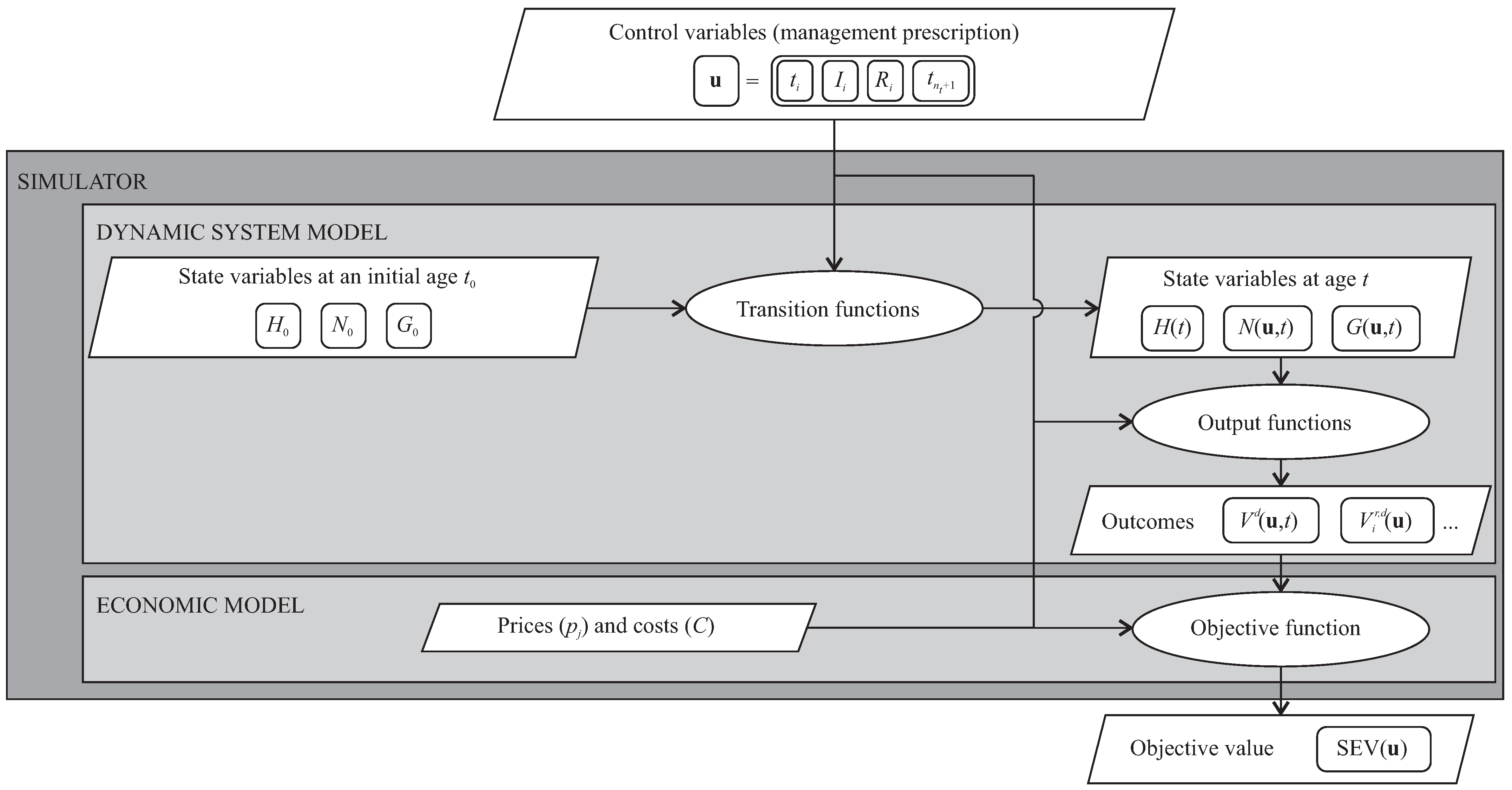
2.1. Optimization Approach

We optimized forest stand management following a similar methodology to that used by Arias-Rodil et al. [26] in the NW of Spain for pure, even-aged stands of Pinus pinaster Ait. In it, the development of a forest stand is simulated using the dynamic systems-based framework (frequently referred to as “state-space” approach) first used in forestry by García [27]. According to it, the forest stand is characterized at each moment by state variables whose evolution, described by time-dependent transition functions, is considered independent of previous states. These functions represent natural dynamics (growth and mortality), are affected by control variables which encapsulate the impact of silvicultural treatments on the state, and are complemented by output functions that translate state variables into outcomes (e.g., timber volume). An economic model provides the objective function value corresponding to these control variables and initial stand conditions (see Figure 1).
We used the most frequent setting under this approach, which characterizes the stand using three state variables: dominant height (mean height of dominant trees in the stand, in metres), H ( t ) , number of stems per hectare, N ( t ) , and stand basal area (total area of stem sections at 1.3 m, in m 2 /ha), G ( t ) . The dynamic of these variables is described by species-specific transition functions h, n, g: R + × R + × R + R , so that, if for an initial age t 0 0 there is a known state where H ( t 0 ) = H 0 , G ( t 0 ) = G 0 and N ( t 0 ) = N 0 , and no silvicultural treatments are applied in [ t 0 , t ] , then it is verified that H ( t ) = h ( t 0 , H 0 , t ) , N ( t ) = n ( t 0 , N 0 , t ) and G ( t ) = g ( t 0 , G 0 , t ) .
Concerning the simulation of silvicultural treatments, each (i-th) thinning is characterized by its intensity (proportion of stems removed), I i , removal relation (ratio between the proportion of stand basal area removed and the proportion of stems removed), R i , and timing, t i . Then, a management prescription is defined by the number of thinnings, n t N , and the vector (control variable) u = ( I 1 , R 1 , t 1 , , I n t , R n t , t n t , t n t + 1 ) R 3 n t + 1 , determining these thinnings and the rotation age t n t + 1 . As R i is usually kept in the interval ( 0 , 1 ] , the dominant height is not affected by treatments (note that a value of R i > 1 would lead to thinning from above). The state variables H ( t ) , N ( u , t ) and G ( u , t ) can be predicted at any age with the transition functions h , n , g , and the control variable u (see [26], for details). Outputs are then obtained from the predicted values of the state variables. For instance, the merchantable timber volume (in m 3 /ha) for a certain product (defined by a limit diameter d, in cm) can be obtained from a known output function v ( H , N , G , d ) : for any t 0 ,
V d ( u , t ) = v H ( t ) , N ( u , t ) , G ( u , t ) , d
gives the merchantable timber volume with diameter greater than d at age t. From this function, the removed timber volume at the i-th thinning is calculated as
V i r , d ( u ) = V d ( u , t i ) V d ( u , t i + ) ,
where t i and t i + denote, respectively, the instants before and after the i-th thinning. In the same way, the removed timber volume at the rotation age is given by
V n t + 1 r , d ( u ) = V d ( u , t n t + 1 ) .
Considering that the purpose is to compare the profitability of management alternatives with different rotation lengths, the economic model considers as objective function the soil expectation value (SEV, [28]):
SEV ( u ) = R ( u ) C ( 1 + r ) t n t + 1 1 ,
where R ( u ) and C are the discounted revenues and costs, and r is the interest rate. For each timber product considered, revenues were computed as the discounted product of stumpage prices and extracted volumes at each thinning and at final harvest:
R ( u ) = i = 1 n t + 1 1 ( 1 + r ) t i j = 1 n a p i j V i r , d j ( u ) V i r , d j + 1 ( u )
where n a is the number of different timber products, V i r , d n a + 1 ( u ) = 0 , I n t + 1 = R n t + 1 = 1 , and p i j is the stumpage price (€/m 3 ) for product j in the i-th cut. If p j is the stumpage price at clearcutting, we assume a depreciation in thinning price due to its lower intensity and, maybe, lower removed relation, such that
p i j = p j a ( 2 R i ) ( 1 I i ) ,
where a > 1 is a parameter that measures the stumpage price depreciation in thinnings.
According to all previous considerations, a simulator for computing the SEV corresponding to each management prescription was developed (see Figure 1). In addition, economic and logistic constraints were considered, and upper and lower bounds for the decision variables were set, determining the admissible set U n t R 3 n t + 1 of possible values of u . Therefore, the forest stand management problem was formulated as the following Mixed-Integer Nonlinear Problem (MINLP):
max SEV ( u )
subject   to u U n t ,
0 n t n t m a x ,
where n t m a x is the maximum number of thinnings allowed.

2.2. Transition Functions and Parameters

As transition functions for estimating the time-dependent changes in the state variables we used the dynamic equations developed by Diéguez-Aranda et al. [29] and Castedo-Dorado et al. [30] for radiata pine in this region:
h ( t 0 , H 0 , t ) = H 0 1 exp ( 0.06738 t ) 1 exp ( 0.06738 t 0 ) 1.755 + 12.44 / A 1 ,
with
A 1 = 0.5 log H 0 + 1.755 A 2 + ( log H 0 + 1.755 A 2 ) 2 49.76 A 2 , A 2 = log 1 exp ( 0.06738 t 0 ) ;
n ( t 0 , N 0 , t ) = ( N 0 0.3161 + 1 . 053 t 100 1 . 053 t 0 100 ) 1 / 0.3161 ;
g ( t 0 , G 0 , t ) = exp ( A 3 ) exp ( 276.1 + 1391 / A 3 ) t 0.9233 ,
with
A 3 = 0.5 t 0 0.9233 276.1 + t 0 0.9233 log ( G 0 ) + 5564 t 0 0.9233 + 276.1 t 0 0.9233 log ( G 0 ) 2 .
The initial values for the before-thinning state were set as follows: (i) for h ( t 0 , H 0 , t ) , t 0 = 20 , which is the reference age for the species according to Diéguez-Aranda et al. [29], and H 0 is the site index (S); (ii) for n ( t 0 , N 0 , t ) , t 0 = 0 and N 0 is the plantation density; and (iii) for g ( t 0 , G 0 , t ) , t 0 = 10 and G 0 is given by
G 0 = exp ( A 4 ) exp ( 276.1 + 1391 / A 4 ) 10 0.9233 ,
with
A 4 = 4.331 S 0.03594 114.3 n ( 0 , N 0 , 10 ) .
Thus, forest productivity was implemented within the simulations through S, which affects the initial basal area and dominant height. The inputs of forest productivity used in this study are explained in Section 2.3.
The output function for the merchantable timber volume was [31]
v ( H , N , G , d ) = 0.4046 H 1.013 G 0.9776 exp ( 0.2933 D g 2.818 d 3.192 ) ,
where the quadratic mean diameter is given by D g = 100 4 G π N .
The necessary information for implementing silvicultural interventions and economic parameters within the simulations was provided by the Spanish forest consultancy company CERNA SL. The proposed management program comprised the initial plantation, scrub clearance, and low pruning. Considering that plantation densities for radiata pine use to vary from 800 to 1100 stems/ha in this region, we chose as initial value for N 0 the mean of that interval, 950 stems/ha. The timber product considered were chip and pulpwood, sawlog and rotary veneer. The cost of management interventions and stumpage prices by product at clearcutting are shown in Table 1. Concerning thinnings, we executed simulations for management prescriptions of one and two thinnings ( n t m a x = 2 ). The constraints for thinning-related decision variables mentioned in Section 2.1 were set as (minimum-maximum): 15%–45% for intensity (I), 0.35 (thinning for below)-1 (systematic thinning) for removal relation (R), and 10–60 years for timing, with a minimal interval of five years between cuttings. Moreover, for discounting the estimated revenues, we compared the results for interest rates of 1%, 3% and 5%.

2.3. Future Forest Productivity

Predictions of S for future climatic scenarios were obtained from a Support Vector Regression (SVR, [32]) model derived from a previous project [33]. The model was developed with data from the research plots network established by the Sustainable Environmental and Forest Management Unit (UXAFORES) of the University of Santiago de Compostela, Spain. As predictors of forest productivity, the model incorporates four variables from the Wordclim 2 bioclimatic dataset [34]: mean annual temperature, mean diurnal range (mean difference between maximum and minimum daily temperatures), isothermality ratio (proportion between mean diurnal range and maximum difference between mean monthly temperatures) and mean temperature of the coldest month. For predicting future S, we used the projections of these four variables developed by the Worldclim project [35] for the period 2041–2060. Specifically, we used the downscaled projections of a set of 11 Global Climate Models (GCMs) included in the Coupled Model Intercomparison Project Phase 5 [36] for the Representative Concentration Pathways (RCPs) 4.5 and 6.0. These pathways represent the forecasted climate dynamics under the assumption of reaching a radiative forcing (proportion of incident solar irradiance and radiated energy from Earth) of 4.5 W/m 2 and 6 W/m 2 , respectively, by the year 2100. The future climatic projections and forest predictivity predictions were obtained for a set of 128 radiata pine stand locations in the northwest of Spain for which current productivity data were available.

2.4. Numerical Resolution and Analysis

Taking into account that only a few thinnings are allowed ( n t m a x is small), MINLP (3)–(5) can be solved by exhaustive search on the integer variable n t . Therefore, for each n t = 1 , , n t m a x , the nonlinear problem (NLP) (3)–(4) is solved with the fixed value of n t , and the best of the n t m a x obtained solutions is taken as the optimal solution of problem (3)–(5).
Concerning to NLP (3)–(4), due to the smoothness of transition functions (6)–(8) and the output function (10), the differentiability of the objective function (1) can be proved (see [26]), and gradient-type methods can be used for solving the problem. In this study, we used the most widespread family: Sequential Quadratic Programming (SQP). Specifically, we used the implementation in the nloptr package [37] of R [38], with a random multi-start and computing gradients by a finite difference method [39]. To speed up calculations, we did parallelization with the doParallel package [40].
The optimizations were executed for the 128 locations assuming n t m a x = 2 . For each location, 22 (11 GCMs and two RCPs) S predictions and three interest rates were considered, leading to a total of 8448 MINLPs (optimization scenarios), i.e., 16,896 NLPs. Finally, we analyzed the empirical distribution of SEV for each location and computed the expected shortfall (ES, [41,42]), a financial risk indicator preferred to other metrics (e.g., the value at risk) for non-normal distributions [43]. Following the definition given by Pfaff [44], we computed ES for a confidence level = 1 α as
ES α = 1 α 0 α q u ( F SEV ) d u ,
where q u ( F SEV ) is the quantile function of the SEV distribution. This indicator can be interpreted as the mean SEV below the quantile defined by α , which we fixed as 0.025 in this study, and that is equivalent to the mean financial loss above the 97.5% threshold, according to the nomenclature used by Pfaff [44]. For discussing the potential sensitiveness of SEV to favorable future climate scenarios, we also computed the symmetric of ES 2.5 , ES 97.5 .
Finally, we compared the SEV estimated for current productivity (assuming no variations in future S, i.e., no climate change), SEV C P , with the mean SEV for climate change scenarios ( SEV C C ¯ ), ES 2.5 and ES 97.5 . In addition, we also tested the economic effect of not adapting silviculture to climate change, i.e., to apply the optimum silvicultural programs for current productivity to RCP 4.5 and RCP 6.0 scenarios (hereafter, “climate-insensitive” silviculture).

3. Results

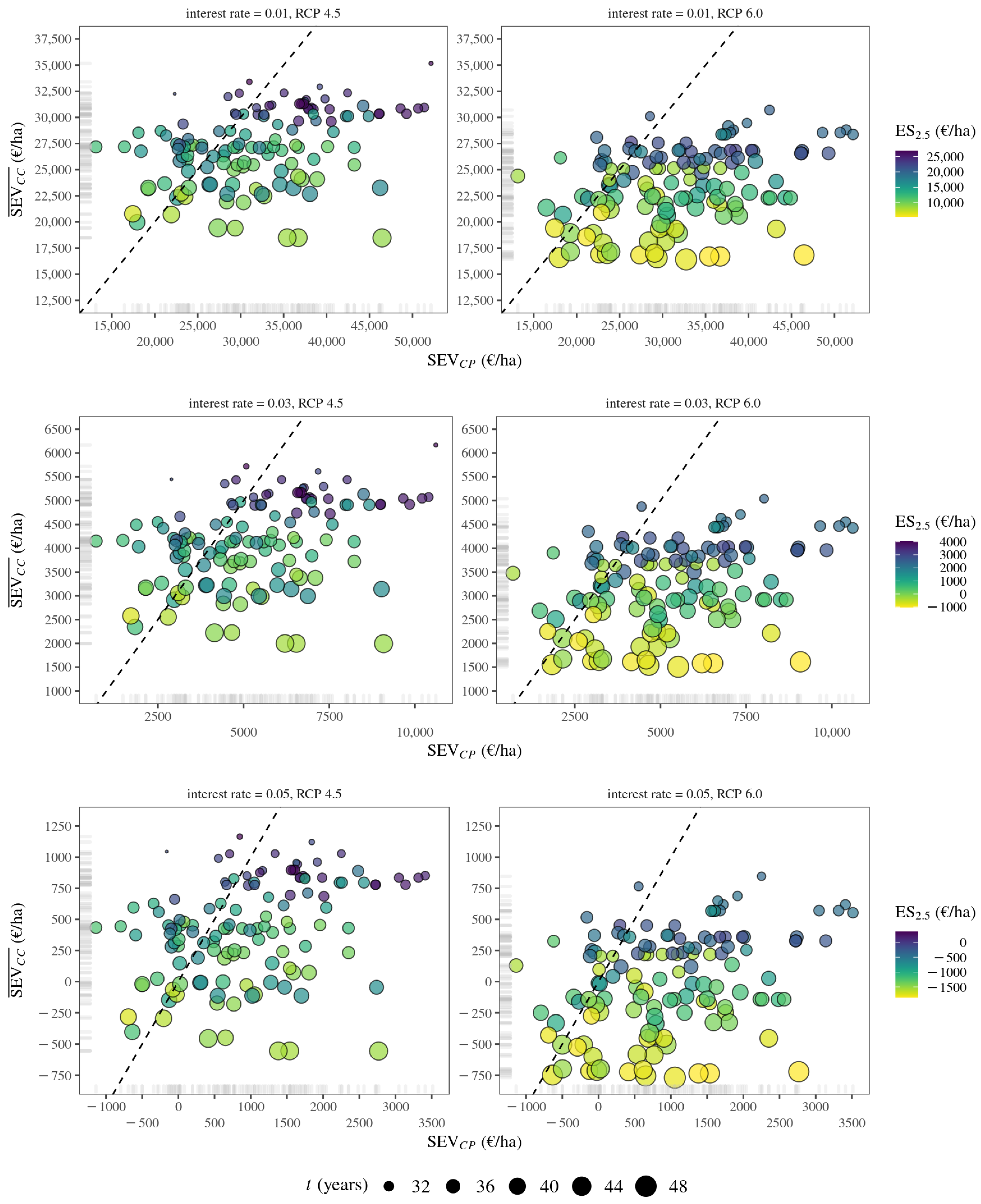
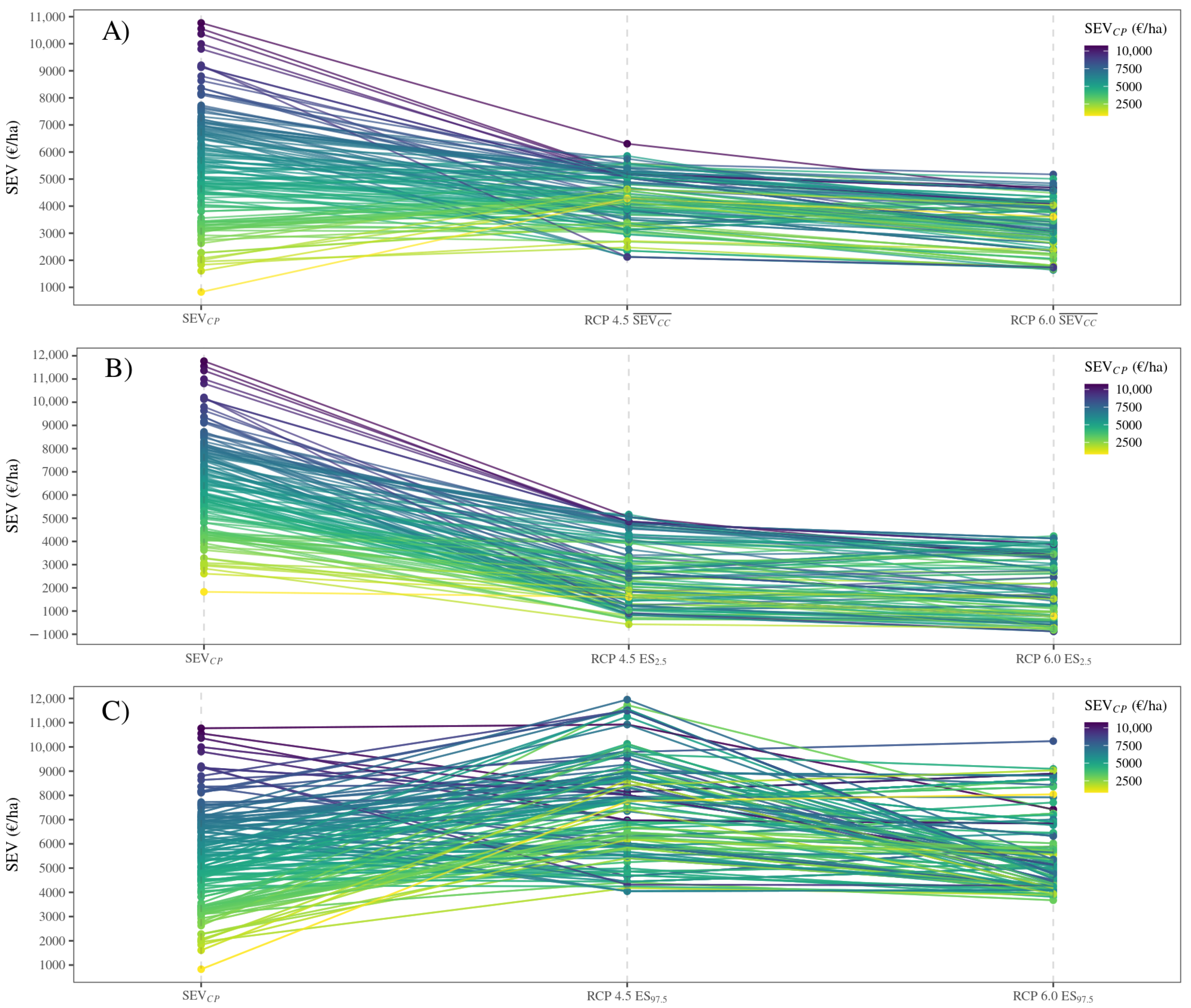
3.1. Productivity and Economic Indicators

The considered future climate models forecasted, on average, an increase in the four S climatic predictors except for the isothermality, which experienced a slight decrease. The most notable shift in climatic variables was the mean temperature of the coldest month, which increased ∼40% with respect to previous conditions. However, these forecasts varied notably over climate models, being the mean temperature of the coldest month the sparsest for both RCPs (relative dispersion ∼15%). The forest productivity predictions derived from these climatic projections revealed a decreasing trend in mean S under climate change. The mean S reduced from 20.8 m (observed productivity) to 18.8 m (RCP 4.5) and 17.3 m (RCP 6.0). Moreover, the variability of these predictions increased notably, with S ranges (min.–max.) of 7.9–32.1 m for RCP 4.5 and 7.1–29.4 m for RCP 6.0 that contrast the observed range of 12.8–27.7 m.
The resulting SEV under optimum silviculture for current productivity varied from −1150 €/ha (for r = 0.05) to ∼52,000 €/ha (for r = 0.01), with a mean value of 12,800 €/ha. Concerning climate change scenarios, the SEV C C ¯ ranged, overall, from −750 to ∼35,000 €/ha with a mean value of 10,500 €/ha for RCP 4.5 and 9000 €/ha for RCP 6.0. With regard to the tails of the SEV C C distribution, the ES 2.5 varied from −1800 €/ha to 27,000 €/ha, while the ES 97.5 varied from 130 €/ha to 56,000 €/ha. Plots of SEV under current productivity vs. SEV under climate change for each interest rate-RCP combination are shown in Figure 2.
As shown in Figure 2, in most of the locations SEV C C ¯ < SEV C P (points are mainly located to the right side of the identity line). In other words, in most locations, simulations under climate change led to a drop in profitability in comparison with the scenario of current productivity. The average relative decrease in profitability from current productivity to climate change scenarios varied in the ranges 15–64% for RCP 4.5 and 22–89% for RCP 6.0. These wide ranges of variation were mostly driven by interest rates, being the highest decreases in profitability associated with high values of r. Increases in SEV from current productivity to climate change (i.e., where SEV C C ¯ > SEV C P ) were scarce and mostly found in some locations with current low-average productivity. A high degree of correspondence was found between SEV C C ¯ and ES 2.5 , meaning that locations with higher SEV C C ¯ had also high ES 2.5 values. However, there were cases with high SEV C C ¯ and low ES 2.5 , and vice versa, which account for the varying dispersion rates of SEV among the different locations. The evolution of SEV from current productivity to SEV C C ¯ , ES 2.5 and ES 97.5 under RCPs 4.5 and 6.0 is shown in Figure 3. Altogether, a descending trend in SEV was noticed in the direction current productivity-RCP 4.5-RCP 6.0. A slightly decreasing trend was also found in ES 2.5 between RCP 4.5 and RCP 6.0. The estimated relative decreases of profitability based on ES 2.5 , from current productivity to climate change scenarios, were of 47–142% (also varying with r) for RCP 4.5 and 55–156% for RCP 6.0. In contrast, ES 97.5 revealed an increase in SEV under climate change scenarios, with relative values of up to 40% for RCP 4.5 and 47% for RCP 6.0.

3.2. Optimum Silviculture

Concerning silvicultural decision variables, the optimum number of thinnnings was one ( n t = 1) in all the optimization scenarios (MINLPs). However, the differences in SEV between optimum silvicultural programs of one and two thinnings were very slight, being the mean difference = 180 €/ha. Climatic scenarios had a noticeable influence on the optimum rotation length, which tended to reach higher values under climate change (RCP 6.0 > RCP 4.5, in most of cases) in comparison to current productivity (Figure 4). As expected, the rotation length also showed a negative correlation with r. The thinning intensities and removal relations were scarcely influenced by climatic scenarios and, overall, experimented low variability. Concerning the first thinning (or the only thinning when n t = 1), the results of most of NLPs yielded values very close to the lower bounds of these decision variables, implying low intensities ( I 1 0.15 ) and thinning from below ( R 1 0.35 ). The optimum intensities of the second thinning (for those NLP with n t = 2) had a broader variation range, with some of the NLPs reaching I 2 0.45 . As with the rotation length, the optimum thinning timings suffered a noticeable variation across optimization scenarios, especially influenced by r. The mean timing for the first thinning was, overall, 19 years and the mean timing of the second thinning was 31 years.

3.3. Results under Climate-Insensitive Silviculture

The use of silvicultural programs calibrated for current productivity under climate change scenarios led, overall, to a noticeable reduction in profitability. This reduction showed a very high variability, which was mainly conditioned by the interest rate, being the worst cases of profitability loss located in scenarios where r = 5 % . These climate-insensitive simulations yielded a mean relative drop in SEV of 2–19% (increasing with r) for RCP 4.5 and 3–39% for RCP 6.0 with respect to silviculture optimized for future climate. The estimated decreases in comparison with the SEV under current productivity were 11–64% (with a maximum of 120 % ) for RCP 4.5 and 22–150% for RCP 6.0.

4. Discussion

The economic simulations carried out in this study indicated a reduction in mean profitability of plantations under climate change. This reduction was caused by a drop in average productivity over climate scenarios which is mainly driven by an increase of temperatures and continentality. The sharpest increase among these climatic drivers was the mean temperature of the coldest month, whose negative impact on site index has already been noticed in previous studies in this region for radiata pine [12] and Scots pine [45]. The main hypothesis for explaining this negative effect is the stress on carbon balance due to high respiration rates during winter, which has also been observed for other pine species [46,47]. Though there is a certain concurrence on the potential effects of climate change on tropical and boreal forests productivity (negative and positive effects, respectively, [48,49,50]), the economic impacts of future climate on temperate forests are still an unclear matter. For instance, according to Alig et al. [51], future forest profitability may be reduced in the southwest of the USA, while Susaeta et al. [52] predict an increase in productivity in the southeast (Florida). We think that our results run parallel to the findings made by Hanewinkel et al. [53], which state that overall, temperate European forests may suffer a severe loss in profitability due to climate change. Specifically, Hanewinkel et al. [53] projected a retreat of pine forests in the northwest of Spain for an expansion of Eucalyptus spp. and Mediterranean oaks. Routa et al. [54] and Serrano-León et al. [55] also predicted a decline in profitability in European pine forests under unfavorable climatic scenarios (e.g., RCP 8.5).
Regarding the observed dispersion in profitability estimations, our comparison between SEV C P and SEV C C ¯ should be taken cautiously given the observed diverging trend between ES 2.5 and ES 97.5 . This trend implies that the dispersion of forest productivity predictions along the different GCMs is high enough to forecast increments and reductions in future profitability alternatively. This fact was already noted by ALRahahleh et al. [56] when analyzing the potential impacts of RCP 4.5 and 8.5 projections on forest growth in Finland. A more detailed assessment of the observed dispersion between GCMs would require a deeper understanding of the mechanisms within the models and downscaled climatic predictions. As ALRahahleh et al. [56] concluded, we believe that the use of a varied set of different GCMs is necessary for realistically representing the underlying uncertainties of forest productivity under future climate. Nevertheless, even considering the yielded dispersion in future financial indicators, our results point out a clear declining trend of average profitability across climatic scenarios (e.g., a decrease of ∼22% for RCP 4.5 and ∼29% for RCP 6.0, with r = 0.03). Considering that the results yielded by both RCPs are notably different (being RCP 6.0, overall, more pessimistic), their implications in terms of financial risks are also distinct. In this regard, despite the existing uncertainty regarding future greenhouse gases emission scenarios, some studies have performed likelihood analyses for assessing the probabilities associated with the different radiative forcing pathways. For instance, Capellán-Pérez et al. [57] used an integrated assessment model for estimating the probability of surpassing the different RCPs by 2100. In their study, Capellán-Pérez et al. [57] report a probability of 92% of surpassing RCP 4.5 and a probability of 42% of surpassing RCP 6.0, being the most likely scenario an intermediate point between both pathways (notably closer to RCP 6.0). Considering these probabilities, a weighted mean of the estimated SEV C C ¯ values for both RCPs would produce an expected loss of ∼28% from current profitability with an interest rate of 3%. The most probable value of ES 2.5 in this context would imply a risk of profitability loss of ∼82%, for the same interest rate.
According to our simulations, optimum silviculture under climate change will consist of longer rotations. Considering the estimated reduction in future mean S under climate change scenarios, this result seems consistent with the negative rotation length–growth rate correlation observed in previous studies [58]. As longer rotations may imply a wider exposure of plantations to disturbances, from a financial perspective this will also lead to potential losses associated with time-dependent risks, such as wildfires. In contrast to some previous studies [59], we did not find a strong sensitivity of thinning intensities and removal relations to interest rates, as they experienced narrow variations across scenarios. However, the optimization of timing decision variables (i.e., thinning timing and rotation length) was decisive for maximizing the SEV across climatic scenarios and interest rates. Even though the greatest variations in SEV were mainly driven by productivity and r, the comparison between optimal and climate-insensitive simulations revealed that silviculture can significantly alleviate part of the profitability losses due to unfavorable climate change conditions. However, the magnitude of this alleviation was strongly dependent on the interest rate (e.g., the drops in SEV were 3–39% for RCP 6.0 when applying suboptimal programs, depending on r). This seems reasonable considering that the major differences between optimal and climate-insensitive programs were timing variables, whose repercussion on the SEV is constrained by r. Consequently, the potential damping effect of silvicultural optimization on profitability losses under climate change might essentially depend on the forest manager’s appreciation of time-dependent risks. If this appreciation leads to high interest rates, optimizing silviculture considering climate change scenarios might be decisive for mitigating economic losses due to unfavorable productivity conditions.
In addition to silvicultural variables, the economic results were also extremely susceptible to interest rates. For instance, for r = 0.01, the ES 2.5 was strictly positive for all the locations, meaning that even under especially unfavorable climatic conditions, the plantations would remain financially feasible. We think that this fact highlights the necessity for correctly calibrating the time value appreciation and, in particular, quantifying its risk-driven components for analyzing forest investments under climate change. Many studies have noted the potential relevance of disturbances such as pests, diseases and wildfires on future forest growth [60], and some have implemented disturbance-derived risks in financial optimization [61], which may be a suitable improvement line for the approach used in this study.

5. Conclusions

In this study, we simulated the financial investment on radiata pine plantations in the northwest of Spain under different climate change scenarios. The maximization of the SEV revealed that future profitability might be, on average, lower than current profitability for most of the simulated forest locations, also finding a decreasing trend from the more favorable radiative forcing scenario (RCP 4.5), to the least favorable one (RCP 6.0). Moreover, the estimated expected shortfall for each location, for a confidence level of 97.5%, pointed out a noticeable risk of even lower profitability. However, the right tail of the projected SEV distribution also showed very high values for some locations, noting that under certain climatic scenarios, future profitability might be higher. A more detailed analysis of the different used Global Climate Models might be necessary for reducing the uncertainty on this matter.
The optimization of silvicultural programs considering future productivity under climate change proved to be useful for mitigating economic losses due to unfavorable climatic conditions. However, this mitigation was extremely dependent on the interest rates. As a consequence, we believe that the convenience of applying specifically optimized silviculture for climate change conditions might also depend on the preferences of the forest managers regarding time-dependent risks.

Author Contributions

Conceptualization, M.A.G.-R., M.E.V.-M. and U.D.-A.; methodology, M.A.G.-R., M.E.V.-M. and U.D.-A.; software, M.A.G.-R.; validation, M.A.G.-R.; formal analysis, M.A.G.-R.; investigation, M.A.G.-R.; resources, M.A.G.-R. and U.D.-A.; data curation, M.A.G.-R.; writing—original draft preparation, M.A.G.-R.; writing—review and editing, M.A.G.-R., M.E.V.-M. and U.D.-A.; visualization, M.A.G.-R.; supervision, M.E.V.-M. and U.D.-A.; project administration, U.D.-A.; funding acquisition, U.D.-A. All authors have read and agreed to the published version of the manuscript.

Funding

This research was funded by the Spanish Ministry of Science and Innovation (grant number DI-16-08971) and by the forest management consultancy company CERNA Ingeniería y Asesoría Medioambiental S.L.

Institutional Review Board Statement

Not applicable.

Informed Consent Statement

Not applicable.

Data Availability Statement

The data underlying in this article is available at the Zenodo repository.

Acknowledgments

The authors thank Worldclim 1.4 and 2 authors [34,35], for the bioclimatic maps provided.

Conflicts of Interest

The authors declare no conflict of interest.

References

  1. Bontemps, J.D.; Bouriaud, O. Predictive approaches to forest site productivity: Recent trends, challenges and future perspectives. Forestry 2014, 87, 109–128. [Google Scholar] [CrossRef]
  2. Lindner, M.; Garcia-Gonzalo, J.; Kolström, M.; Green, T.; Reguera, R.; Maroschek, M.; Seidl, R.; Lexer, M.J.; Netherer, S.; Schopf, A.; et al. Impacts of Climate Change on European Forests and Options for Adaptation; Report to the European Commission Directorate-General for Agriculture and Rural Development; JFNW: Joensuu, Finland, 2008. [Google Scholar]
  3. Bussotti, F.; Pollastrini, M.; Holland, V.; Brüggemann, W. Functional traits and adaptive capacity of European forests to climate change. Environ. Exp. Bot. 2015, 111, 91–113. [Google Scholar] [CrossRef]
  4. Thurm, E.A.; Hernandez, L.; Baltensweiler, A.; Ayan, S.; Rasztovits, E.; Bielak, K.; Zlatanov, T.M.; Hladnik, D.; Balic, B.; Freudenschuss, A.; et al. Alternative tree species under climate warming in managed European forests. For. Ecol. Manag. 2018, 430, 485–497. [Google Scholar] [CrossRef]
  5. Brecka, A.F.; Shahi, C.; Chen, H.Y. Climate change impacts on boreal forest timber supply. For. Policy Econ. 2018, 92, 11–21. [Google Scholar] [CrossRef]
  6. Mei, B.; Clutter, M.L.; Harris, T.G. Timberland Return Drivers and Timberland Returns and Risks: A Simulation Approach. South. J. Appl. For. 2013, 37, 18–25. [Google Scholar] [CrossRef]
  7. Sonwa, D.J.; Somorin, O.A.; Jum, C.; Bele, M.Y.; Nkem, J.N. Vulnerability, forest-related sectors and climate change adaptation: The case of Cameroon. For. Policy Econ. 2012, 23, 1–9. [Google Scholar] [CrossRef]
  8. Fontes, L.; Bontemps, J.D.; Bugmann, H.; Van Oijen, M.; Gracia, C.; Kramer, K.; Lindner, M.; Rotzer, T.; Skovsgaard, J.P. Models for supporting forest management in a changing environment. For. Syst. 2010, 19, 8–29. [Google Scholar] [CrossRef] [Green Version]
  9. Skovsgaard, J.P.; Vanclay, J.K. Forest site productivity: A review of the evolution of dendrometric concepts for even-aged stands. Forestry 2008, 81, 13–31. [Google Scholar] [CrossRef] [Green Version]
  10. Aertsen, W.; Kint, V.; van Orshoven, J.; Özkan, K.; Muys, B. Comparison and ranking of different modelling techniques for prediction of site index in Mediterranean mountain forests. Ecol. Model. 2010, 221, 1119–1130. [Google Scholar] [CrossRef]
  11. Sabatia, C.O.; Burkhart, H.E. Predicting site index of plantation loblolly pine from biophysical variables. For. Ecol. Manag. 2014, 326, 142–156. [Google Scholar] [CrossRef]
  12. González-Rodríguez, M.; Diéguez-Aranda, U. Exploring the use of learning techniques for relating the site index of radiata pine stands with climate, soil and physiography. For. Ecol. Manag. 2020, 458. [Google Scholar] [CrossRef]
  13. Roessiger, J.; Griess, V.C.; Knoke, T. May risk aversion lead to near-natural forestry? A simulation study. Forestry 2011, 84, 527–537. [Google Scholar] [CrossRef] [Green Version]
  14. Pukkala, T.; Kellomäki, S. Anticipatory vs. adaptive optimization of stand management when tree growth and timber prices are stochastic. Forestry 2012, 85, 463–472. [Google Scholar] [CrossRef] [Green Version]
  15. Hahn, W.A.; Härtl, F.; Irland, L.C.; Kohler, C.; Moshammer, R.; Knoke, T. Financially optimized management planning under risk aversion results in even-flow sustained timber yield. For. Policy Econ. 2014, 42, 30–41. [Google Scholar] [CrossRef]
  16. Mei, B.; Wear, D.N.; Henderson, J.D. Timberland investment under both financial and biophysical risk. Land Econ. 2019, 95, 279–291. [Google Scholar] [CrossRef]
  17. Pasalodos-Tato, M. Optimising forest stand management in Galicia, north-western Spain. Diss. For. 2010, 2010. [Google Scholar] [CrossRef] [Green Version]
  18. Arimizu, T. Regulation of the cut by dynamic programming. J. Oper. Res. Soc. Jpn. 1958, 1, 175–182. [Google Scholar]
  19. Valsta, L.T. A comparison of numerical methods for optimizing even aged stand management. Can. J. For. Res. 1990, 20, 961–969. [Google Scholar] [CrossRef]
  20. Kao, C.; Brodie, J. Simultaneous optimisation of thinning and rotation with continuous stocking and entry intervals. For. Sci. 1980, 26, 338–346. [Google Scholar]
  21. Valsta, L. Stand Management Optimization Based on Growth Simulators; Research Paper 453; Finnish Forest Research Institute: Joensuu, Finland, 1993. [Google Scholar]
  22. Hooke, R.; Jeeves, T.A. “Direct Search” Solution of Numerical and Statistical Problems. J. ACM 1961, 8, 212–229. [Google Scholar] [CrossRef]
  23. Storn, R.; Price, K. Differential Evolution—A Simple and Efficient Heuristic for global Optimization over Continuous Spaces. J. Glob. Optim. 1997, 11, 341–359. [Google Scholar] [CrossRef]
  24. Kennedy, J.; Eberhart, R. Particle swarm optimization. In Proceedings of the ICNN’95—International Conference on Neural Networks, Perth, WA, Australia, 27 November–1 December 1995; IEEE: New York, NY, USA, 1995; Volume 4, pp. 1942–1948. [Google Scholar] [CrossRef]
  25. Beyer, H.G.; Schwefel, H.P. Evolution strategies – A comprehensive introduction. Nat. Comput. 2002, 1, 3–52. [Google Scholar] [CrossRef]
  26. Arias-Rodil, M.; Diéguez-Aranda, U.; Vázquez-Méndez, M. A differentiable optimization model for the management of single-species, even-aged stands. Can. J. For. Res. 2017, 47, 506–514. [Google Scholar] [CrossRef] [Green Version]
  27. García, O. The state-space approach in growth modelling. Can. J. For. Res. 1994, 24, 1894–1903. [Google Scholar] [CrossRef]
  28. Bettinger, P.; Boston, K.; Siry, J.P.; Grebner, D.L. Forest Management and Planning, 2nd ed.; Elsevier Inc.: Amsterdam, The Netherlands, 2017; pp. 1–349. [Google Scholar]
  29. Diéguez-Aranda, U.; Burkhart, H.E.; Rodríguez-Soalleiro, R. Modeling dominant height growth of radiata pine (Pinus radiata D. Don) plantations in north-western Spain. For. Ecol. Manag. 2005, 215, 271–284. [Google Scholar] [CrossRef]
  30. Castedo-Dorado, F.; Diéguez-Aranda, U.; Álvarez-González, J.G. A growth model for Pinus radiata D. Don stands in north-western Spain. Ann. For. Sci. 2007, 64, 453–465. [Google Scholar] [CrossRef] [Green Version]
  31. Arias-Rodil, M.; Romero-Martínez, P.; Diéguez-Aranda, U. Estimación Delvolumen Comercial a Partir de Variables de Rodal; 7° Congreso Forestal Español; Sociedad Española de Ciencias Forestales: Plasencia, Spain, 2017. [Google Scholar]
  32. Vapnik, V.; Golowich, S.; Smola, A. Support vector method for function approximation, regression estimation, and signal processing. In Advances in Neural Information Processing Systems, 9th ed.; Mozer, M., Jordan, M., Petsche, T., Eds.; MIT Press: Cambridge, MA, USA, 1997; pp. 281–287. [Google Scholar] [CrossRef]
  33. González-Rodríguez, M.; Diéguez-Aranda, U. Delimiting the spatio-temporal uncertainty of climate-sensitive forest productivity projections using Support Vector Regression. Ecol. Indic. 2021, 128. [Google Scholar] [CrossRef]
  34. Fick, S.E.; Hijmans, R.J. WorldClim 2: New 1-km spatial resolution climate surfaces for global land areas. Int. J. Climatol. 2017, 37, 4302–4315. [Google Scholar] [CrossRef]
  35. Hijmans, R.J.; Cameron, S.E.; Parra, J.L.; Jones, P.G.; Jarvis, A. Very high resolution interpolated climate surfaces for global land areas. Int. J. Climatol. 2005, 25, 1965–1978. [Google Scholar] [CrossRef]
  36. Taylor, K.E.; Stouffer, R.J.; Meehl, G.A. An overview of CMIP5 and the experiment design. Bull. Am. Meteorol. Soc. 2012, 93, 485–498. [Google Scholar] [CrossRef] [Green Version]
  37. Johnson, S.G. The NLopt Nonlinear-Optimization Package (Version 1.2.2.2). Available online: http://ab-initio.mit.edu/nlopt (accessed on 2 July 2020).
  38. R Development Core Team. R: A Language and Environmental for Estatistical Computing (Version 4.1.0); R Foundation for Statistical Computing: Vienna, Austria, 2021; Available online: https://www.R-project.org/ (accessed on 18 May 2021).
  39. Nocedal, J.; Wright, S. Numerical Optimization; Springer Series in Operations Research and Financial Engineering; Springer: New York, NY, USA, 2006. [Google Scholar] [CrossRef] [Green Version]
  40. Microsoft Corporation and Steve Weston. doParallel: Foreach Parallel Adaptor for the ‘parallel’ Package (Version 1.0.14). Available online: https://CRAN.R-project.org/package=doParallel (accessed on 24 September 2018).
  41. Artzner, P.; Delbaen, F.; Eber, J.M.; Heath, D. Thinking coherently, Risk magazine. Risk Mag. 1997, 10, 68–71. [Google Scholar]
  42. Artzner, P.; Delbaen, F.; Eber, J.M.; Heath, D. Coherent Measures of Risk. Math. Financ. 1999, 9, 203–228. [Google Scholar] [CrossRef]
  43. Yamai, Y.; Yoshiba, T. Value-at-risk versus expected shortfall: A practical perspective. J. Bank. Financ. 2005, 29, 997–1015. [Google Scholar] [CrossRef]
  44. Pfaff, B. Financial Risk Modelling and Portfolio Optimization with R; John Wiley & Sons, Ltd.: Chichester, UK, 2016; pp. 1–426. [Google Scholar] [CrossRef]
  45. González-Rodríguez, M.Á.; Diéguez-Aranda, U. Rule-based vs. parametric approaches for developing climate-sensitive site index models: A case study for Scots pine stands in northwestern Spain. Ann. For. Sci. 2021, 78, 23. [Google Scholar] [CrossRef]
  46. Valkonen, M.L.; Hänninen, H.; Pelkonen, P.; Repo, T. Frost hardiness of Scots pine seedlings during dormancy. Silva Fennica. 1990, 24, 335–340. [Google Scholar] [CrossRef] [Green Version]
  47. Wu, L.; Hallgren, S.W.; Ferris, D.M.; Conway, K.E. Effects of moist chilling and solid matrix priming on germination of loblolly pine (Pinus taeda L.) seeds. New For. 2001, 21, 1–16. [Google Scholar] [CrossRef]
  48. Salafsky, N. Drought in the rain forest: Effects of the 1991 El Niño-Southern Oscillation event on a rural economy in West Kalimantan, Indonesia. Clim. Chang. 1994, 27, 373–396. [Google Scholar] [CrossRef]
  49. van Kooten, G.C. Climate Change Impacts on Forestry: Economic Issues. Can. J. Agric. Econ. Can. D’Agroeconomie 1990, 38, 701–710. [Google Scholar] [CrossRef]
  50. Feeley, K.J.; Wright, S.J.; Nur Supardi, M.N.; Kassim, A.R.; Davies, S.J. Decelerating growth in tropical forest trees. Ecol. Lett. 2007, 10, 461–469. [Google Scholar] [CrossRef]
  51. Alig, R.J.; Adams, D.M.; McCarl, B.A. Projecting impacts of global climate change on the US forest and agriculture sectors and carbon budgets. For. Ecol. Manag. 2002, 169, 3–14. [Google Scholar] [CrossRef]
  52. Susaeta, A.; Adams, D.C.; Carter, D.R.; Gonzalez-Benecke, C.; Dwivedi, P. Technical, allocative, and total profit efficiency of loblolly pine forests under changing climatic conditions. For. Policy Econ. 2016, 72, 106–114. [Google Scholar] [CrossRef] [Green Version]
  53. Hanewinkel, M.; Cullmann, D.A.; Schelhaas, M.J.; Nabuurs, G.J.; Zimmermann, N.E. Climate change may cause severe loss in the economic value of European forest land. Nat. Clim. Chang. 2013, 3, 203–207. [Google Scholar] [CrossRef]
  54. Routa, J.; Kilpeläinen, A.; Ikonen, V.P.; Asikainen, A.; Venäläinen, A.; Peltola, H. Effects of intensified silviculture on timber production and its economic profitability in boreal Norway spruce and Scots pine stands under changing climatic conditions. For. Int. J. For. Res. 2019, 92, 648–658. [Google Scholar] [CrossRef] [Green Version]
  55. Serrano-León, H.; Ahtikoski, A.; Sonesson, J.; Fady, B.; Lindner, M.; Meredieu, C.; Raffin, A.; Perret, S.; Perot, T.; Orazio, C. From genetic gain to economic gain: Simulated growth and financial performance of genetically improved Pinus sylvestris and Pinus pinaster planted stands in France, Finland and Sweden. For. Int. J. For. Res. 2021. [Google Scholar] [CrossRef]
  56. ALRahahleh, L.; Kilpeläinen, A.; Ikonen, V.P.; Strandman, H.; Venäläinen, A.; Peltola, H. Effects of CMIP5 Projections on Volume Growth, Carbon Stock and Timber Yield in Managed Scots Pine, Norway Spruce and Silver Birch Stands under Southern and Northern Boreal Conditions. Forests 2018, 9, 208. [Google Scholar] [CrossRef] [Green Version]
  57. Capellán-Pérez, I.; Arto, I.; Polanco-Martínez, J.M.; González-Eguino, M.; Neumann, M.B. Likelihood of climate change pathways under uncertainty on fossil fuel resource availability. Energy Environ. Sci. 2016, 9, 2482–2496. [Google Scholar] [CrossRef] [Green Version]
  58. Palahí, M.; Pukkala, T. Optimising the management of Scots pine (Pinus sylvestris L.) stands in Spain based on individual-tree models. Ann. For. Sci. 2003, 60, 105–114. [Google Scholar] [CrossRef]
  59. Pukkala, T. Instructions for optimal any-aged forestry. For. Int. J. For. Res. 2018, 91, 563–574. [Google Scholar] [CrossRef]
  60. Kirilenko, A.P.; Sedjo, R.A. Climate change impacts on forestry. Proc. Natl. Acad. Sci. USA 2007, 104, 19697–19702. [Google Scholar] [CrossRef] [PubMed] [Green Version]
  61. Susaeta, A.; Carter, D.R.; Chang, S.J.; Adams, D.C. A generalized Reed model with application to wildfire risk in even-aged Southern United States pine plantations. For. Policy Econ. 2016, 67, 60–69. [Google Scholar] [CrossRef] [Green Version]
Figure 1. Flow diagram of the simulator developed for computing the objective value (SEV) of a given management prescription.
Forests 12 00899 g001
Figure 2. Scatterplots of SEV under current productivity ( SEV C P ) vs. mean SEV under climate change for the two RPC’s and the three interest rates considered. The dashed line in each plot represents the identity.
Forests 12 00899 g002
Figure 3. Parallel coordinates plots representing the change from SEV under current productivity ( SEV C P ) to (A) mean SEV under climate change ( SEV C C ¯ ), (B) future ES 2.5 and (C) future ES 97.5 for an interest rate = 0.03.
Forests 12 00899 g003
Figure 4. Violin plot of optimum rotation length vs. climatic scenario (Current productivity, RCP 4.5 and RCP 6.0).
Forests 12 00899 g004
Table 1. Economic parameters used for the simulations.
DescriptionValue
CostsPlantation ( t = 0 )1300 €/ha
Scrub clearing ( t = 3 )450 €/ha
Scrub clearing ( t = 10 )450 €/ha
Low pruning ( t = 10 )750 €/ha
PricesChip and pulpwood ( d 1 = 7 cm)16 €/m 3
Sawlog ( d 2 = 16 cm)24 €/m 3
Rotary veneer ( d 3 = 25 cm)30 €/m 3
Stumpage price depreciation parameter in thinnings2
Publisher’s Note: MDPI stays neutral with regard to jurisdictional claims in published maps and institutional affiliations.

