Modeling the Diameter Distribution of Mixed Uneven-Aged Stands in the South Western Carpathians in Romania

Abstract

Tree diameter measurements are repetitive, time-consuming, and laborious but necessary to obtain the diameter distribution of the stands. Tree diameter distribution provides much of the information necessary for sustainable management and can be predicted with high accuracy, thus saving time and financial resources. Permanent sample plots that belong to a permanent sampling network located in a protected area in the South Western Carpathians in Romania were used in this study. We compared two theoretical distribution functions and predicted or recovered their parameters using parameter prediction and parameter recovery methods. Five modeling approaches based on maximum likelihood and the method of moments were used to predict the diameter distribution of unmanaged mixed uneven-aged stands. Parameter recovery methods outperformed parameter prediction methods while the left-truncated Weibull distribution outperformed the complete Weibull distribution. The accuracy obtained by the best modeling approach measured by the relative root mean squared error (%RMSE) reaches up to 12.6% when the sums of the diameters are raised to the third power and only 0.02% and 4.8% for the sums of the second powers and the sum of the diameters respectively. This research is the first of this kind in Romania and can serve as an example of alternative solutions to the yield tables in estimating the volume of mixed uneven-aged stands and can be easily implemented into forest growth models to predict the diameter distribution in the absence of tree lists.

1. Introduction

Sustainable management of local, regional, or national forest resources is conditioned by the knowledge of the size and structure of forest resources. Knowing these two characteristics, one can ensure that the applied forest management will secure the continuity of the forest ecosystem.

Wood is one of the most important natural resources [1] and its size is usually measured in cubic meters. The size of wood resources is a consequence of the stands’ structure, the species mixture, and their productivity. Stand structure is given by the overall image of the stand [2]. It can be characterized through the vertical and horizontal distribution of trees characteristics, including tree heights and diameters of dead and alive trees [3]. The number of trees per diameter class, also known as diameter distribution, is generally used to describe the stand structure.

Tree diameter distribution is one of the most important aspects to be considered by forest managers when making decisions about the management of forest stands as it provides a wide range of information, from timber assortments to carbon stock and even forest biodiversity [4]. Since the diameter distribution of a stand is determined based on samples with a large number of trees, different methods have been developed to reduce the necessary sampling and ease the diameter distribution determination [5,6]. The diameter distributions have been widely associated with different probability functions [7,8,9,10,11,12] although non-parametric methods as percentile-based, k-nearest neighbor, or artificial neural networks methods have also been used [13,14,15,16]. Alternative methods that have been successfully applied in uneven-aged stands include the use of decreasing geometric progression [17] and negative exponential equation [18], with the two expressions leading to the same results being mathematically equivalent. Due to its flexibility and the simplicity of interpreting and predicting the parameters of the function, the Weibull probability function [8] has been widely applied both in even-aged and uneven-aged forests [10,12,19,20]. Furthermore, the Weibull distribution (WD) probability function is used in forest growth simulators such as SILVA [21,22] or BWIN [23] to predict the diameter distribution of forest stands based on stand characteristics and regression techniques. A special case of the WD is its left-truncated form (LTWD) [24] which has found its application in forest inventories that have a pre-defined recording limit [12,25].

Parameter prediction and parameter recovery are the most frequently used methods to obtain the Weibull function parameters based on stand characteristics. Although over the years, plenty of models have been developed across Europe to predict or recover the parameters of WD in even and uneven-aged stands, these methods have not yet been applied to the Romanian forests. Moreover, limited information is available on the method’s applicability and accuracy in mixed unmanaged uneven-aged stands. The aim of this research is (1) to test and compare the complete WD with the LTWD for describing the diameter distribution of mixed unmanaged uneven-aged stands in the south-western Carpathians in Romania and (2) to establish the best method to predict their parameters.

2. Materials and Methods

2.1. Study Area and Field Design

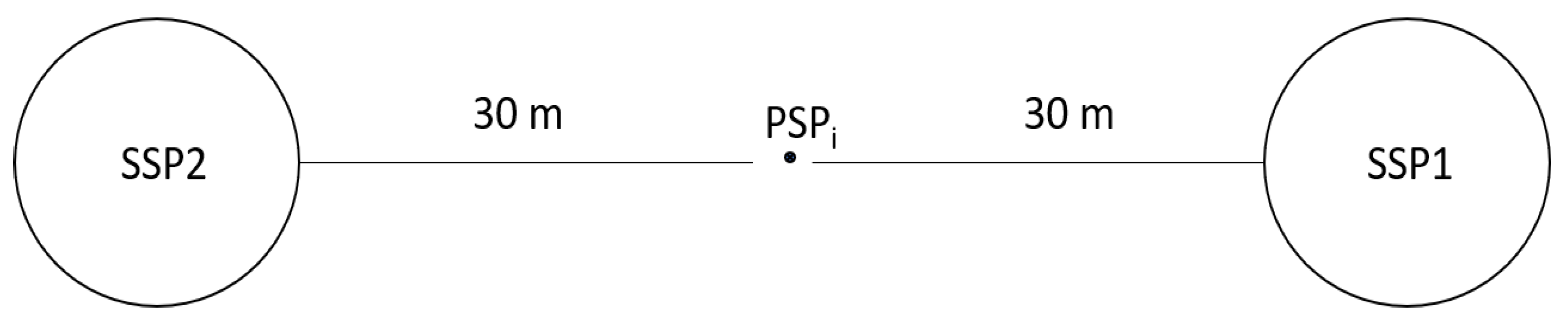
This research focuses on the Retezat National Park (RNP) which is a 3805 km² protected area located in the south-western Carpathians in Romania. A permanent sampling network (PSN) was designed and installed in 2015 and remeasured in the summer of 2020. The permanent sampling network is designed as a 400 × 400 m grid which resulted in 178 permanent sampling plots (PSP). Each PSP consists of two circular subsampling plots (SSP) at a 30 m distance between them and the center of the PSP (Figure 1).

The diameters were sampled starting from 8 cm, which is the minimum diameter measured in each SSP, and the height was measured for a subsample of trees, at least one for each diameter class. The size of the SSPs varied based on the maximum diameter at the breast height (d): 200 m² if the maximum diameter was <28 cm or 500 m² otherwise. More on the study area, sampling design, and the data sampling procedure can be found in reference [26].

Knowing that the number of trees plays a major role in accurately assessing the diameter distribution of the stand [27], only PSPs with at least 50 trees and 1000 m² were selected for the fitting dataset. The data from both measurements (2015 and 2020) were used in this analysis resulting in 103 PSPs selected (

Table 1. Number of PSPs based on the mixture classes.

Species/Group	Species Mixture (Number of PSP’s)
	1–24%	25–49%	50–74%	75–100%
SPR		14	20	54
BE	24	15	10	2
FIR	33	10	6
HB	38	1
SB	40	3
OC	11

Where SPR—spruce, BE—beech, FIR—fir, HB—hardwood broadleaves, SB—softwood broadleaves, OC—other conifers. The species share in each PSP was determined based on the number of trees per hectare.

). The PSPs selected were dominated by spruce in a mixture of beech and fir while hardwood broadleaves, softwood broadleaves, and other conifers were scattered throughout the PSPs. The main characteristics of the dataset are presented in

Table 2. Species main biometric characteristics of the fitting dataset.

Species/Group	$\overline{\mathit{d}}$	dg	med	s	CV	min	max	N
SPR	26.7	30.3	23.6	14.3	53.8	8.0	135.3	6129
BE	29.3	35.4	21.7	19.8	67.6	8.0	121.0	844
FIR	31.0	37.3	24.4	20.7	66.8	8.2	106.1	653
HB	32.3	37.2	28.6	18.5	57.1	10.4	91.5	121
SB	20.2	22.7	17.8	10.2	50.7	8.1	60.3	296
OC	35.2	38.3	34.3	15.3	43.6	8.2	63.9	50

Where $\overline{d}$—arithmetic mean diameter, dg—quadratic mean, med—median diameter, s—standard deviation, CV—diameter coefficient of variation, min and max—minimum and maximum diameter, and N—number of trees measured.

.

A test dataset was used to validate the distributions and methods selected. This dataset consists of two experimental plots of one hectare each (100 × 100 m) fully inventoried both in 2012 and 2019, another experimental plot of one hectare fully inventoried in 2014, and 12 plots of one hectare partially inventoried in a cluster of 5 subplots of 500 m² each, placed on cardinal directions (N, E, S, W) and in the center of the plot. The first two fully inventoried areas were pure SPR and BE (BE- beech) stands (GMO, GFA). The second fully inventoried area (ZNG) was dominated by BE (45%) mixed with SPR, FIR, and HB. The 12 partially inventoried areas were mixed stands of SPR with OC, HB, SB, FIR, BE in the same proportion (P1, P6, P9, P11); SPR in a percentage of over 75% (P2, P3, P5, P10) mixed with other groups of species; SPR in a percentage of over 60% mixed with only with FIR and BE (P4, P7); and BE in a percentage of over 75% (P8, P12) mixed with other groups of species.

2.2. Weibull and Truncated Weibull

The Weibull probability density function (pdf) is described by parameters $\alpha$, b, and c, also known as location, scale, and shape parameters. Since the location parameter is equal to the minimum diameter found in the PSP, and knowing that the value of the minimum diameter varies above the imposed threshold by chance, as well as taking into account that rationally the function should start from 0, we replaced the location parameter $\alpha$ with 0 to obtain the Weibull 2 parameters (W2P) probability density function (Equation (1)).

$$\begin{array}{c}f\left(d\right)=\frac{c}{b}{\left(\frac{d}{b}\right)}^{c-1}{e}^{-{\left(\frac{d}{b}\right)}^c}\\ (d\ge 0;c,b>0)\end{array}$$

(1)

where $f\left(d\right)$ is the probability density function of the trees with the size d $\left(0\le d\right)$, while b and c are the parameters of the function.

Knowing that our data is censored under 8 cm, an additional parameter T is required to obtain the left-truncated Weibull (WT2P) probability density function (Equation (2)).

$$\begin{array}{c}{f}_T\left(d\right)=\frac{c}{b}{\left(\frac{d}{b}\right)}^{c-1}{e}^{\left(\frac{T^c-d^c}{b^c}\right)}\\ \left(T\le d\langle \infty ,T,c,b\rangle 0\right)\end{array}$$

(2)

where: $f_T\left(d\right)$ is the probability density function of the WT2P, T represents the truncation limit which in our case is 8 cm and the other parameters were explained above.

The cumulative probability density function of the W2P and WT2P are given by Equations (3) and (4).

$$\begin{array}{c}F\left(d\right)=1-e^{-{\left(\frac{d}{b}\right)}^c}\\ (d\ge 0;c,b>0)\end{array}$$

(3)

$$\begin{array}{c}{F}_T\left(d\right)=1-e^{{\left(\frac{T}{b}\right)}^c}{e}^{-{\left(\frac{d}{b}\right)}^c}\\ \left(T\le d\langle \infty ,T,c,b\rangle 0\right)\end{array}$$

(4)

2.3. Parameter Prediction Method

Two methods of the PPM were used in this study by applying 4 modeling approaches (M1–M4). The classic three steps method involves choosing a frequency function, obtaining the parameters of the function for each PSP, and estimating regression models that explain the variation of the parameters using stand characteristics [28]. For this method, the parameters of the model were estimated using maximum likelihood (ML) hereafter M1, and the method of moments (MM) hereafter M2. The negative log-likelihood function was minimized using the mle function of the stats4 package in R [29,30] while the method of moments was applied following the methodology proposed by Merganič and Sterba [19]. The M2 method estimates the parameters of the function using the arithmetic mean diameter (AMD) and quadratic mean diameter (QMD). Using these two moments, the standard deviation (SD) and the coefficient of variation (CV) are computed. Parameters b and c were obtained by iteratively changing the values of b in Equations (5) and (6) and c in Equation (7) until we obtained the PSP’s QMD and the CV.

$$QMD=\sqrt{b^2\mathsf{\Gamma }\left(1+\frac{2}{c}\right)}$$

(5)

$$QMD=\sqrt{{{\displaystyle \int }}_T^{\infty }{d}^2{f}_T\left(d\right)dx}$$

(6)

$$CV=\left(\frac{\sqrt{2\mathsf{\Gamma }\left(\frac{c+2}{c}\right)-2\sqrt{\mathsf{\Gamma }\left(\frac{c+2}{c}\right)}\mathsf{\Gamma }\left(\frac{c+1}{c}\right)}}{\sqrt{\mathsf{\Gamma }\left(\frac{c+2}{c}\right)}}\right)100$$

(7)

where $\mathsf{\Gamma }()$ is the complete gamma function, while the other elements were explained above. The first step was to iteratively estimate parameter c until the left side of Equation (7) became equal to the CV of the PSP for which the parameters were computed. Then Equation (5) was applied for determining the b parameter of the W2P function while Equation (6) was applied for determining the b parameter of the WT2P function.

Stand characteristics and seemingly unrelated regression [31] were used to explain the parameters variation obtained with M1 and M2.

The second PPM method bypasses the individual estimation of the parameters. It is based on method 6 described in Cao [32] and its objective is to minimize the following weighted sum of plot-specific log-likelihoods [30,33]:

$$\ell \left(\mathsf{{\rm Y}}\right)={\displaystyle \sum }_{i=1}^N\frac{1}{n_i}{\displaystyle \sum }_{j=1}^{n_i}\log f\left(d_{ij}|\exp (x_i{}^{\left(b\right),}{\mathsf{{\rm Y}}}_b\right),\exp (x_i{}^{\left(c\right)}{\mathsf{{\rm Y}}}_c))$$

(8)

where: $\exp \left(x_i{}^{\left(b\right),}{\mathsf{{\rm Y}}}_b\right)$ and $\exp \left(x_i{}^{\left(c\right),}{\mathsf{{\rm Y}}}_c\right)$ are the functions used to explain the W2P and the WT2P parameter variation, ${\mathsf{{\rm Y}}}_b,{\mathsf{{\rm Y}}}_c$ are the regression coefficients, $x_i{}^{\left(b\right)}$ and $x_i{}^{\left(c\right)}$ are vectors of stand-specific characteristics of PSP i, $f(d|b,c)$ is pdf of W2P and WT2P, N is the number of PSP, and $n_i$ the number of trees of PSP i. This method is referred to in the text hereafter as M3. Another method (M4) was used by removing the weighting of stand specific likelihoods $\left(\frac{1}{n}\right)$ from Equation (8). An example of the implementation of both functions in R [29] is provided in [30] while the implementation of the algorithm for M2 in R is given in Appendix A.

2.4. Parameter Recovery Method

Considering that the estimation of W2P and WT2P parameters using the method of moments is based only on AMD and QMD see [19], a regression equation was developed to predict the AMD based on stand-specific characteristics and QMD. The equation was developed knowing that the QMD is easier to be obtained based on relascope estimation [34] than AMD. Based on the predicted AMD $\left(\widehat{AMD}\right)$ and the measured QMD, the parameters of W2P and WT2P were estimated (M5) using the procedure described for M2. The equation developed was evaluated using the root mean squared error (RMSE) and mean error statistic (ME).

$$RMSE=\sqrt{\frac{{\sum }_{i=1}^N{\left(AMD-\widehat{AMD}\right)}^2}{N-1}}$$

(9)

$$ME=\frac{{\sum }_{i=1}^N\left(AMD-\widehat{AMD}\right)}{N-1}$$

(10)

where N is the number of PSPs and the other elements were described above.

2.5. Evaluation of the Functions and Methods Used

The methods and functions were evaluated using two dispersion measures of the predicted values compared to the experimental values. Relative biases and the square root of mean squared error (RMSEs) were calculated using Equations (9) and (10) [9,10,35].

$$\%Bia{s}^c=100\times \frac{{\sum }_{j=1}^N\left(D_j^c-{\widehat{D}}_j^c\right)}{N-1}\times \frac{1}{{\sum }_j^N{\widehat{D}}_j^c/N}$$

(11)

$$\%RMS{E}^c=100\times \sqrt{\frac{{\sum }_{j=1}^N{\left(D_j^c-{\widehat{D}}_j^c\right)}^2}{N-1}}\times \frac{1}{{\sum }_j^N{\widehat{D}}_j^c/N}$$

(12)

where: N is the number of PSPs, $D_j^c$ is the sum of the diameters of the experimental distribution calculated using Equation (13), ${\widehat{D}}_j^c$ is the predicted sum of the diameters obtained by fitting W2P and WT2P functions, and c is the power the sum of diameters is being raised and varies from 0 to 3.

$$D_j^c={\displaystyle \sum }_{i=1}^{n_j}{n}_{ij}{d}_{ij}^c$$

(13)

$n_j$ is the number of trees from PSP j, $n_{ij}$ is the number of trees per hectare corresponding to tree i from PSP j, with the diameter of value d.

Using the estimated parameters, the number of trees was calculated for 1 cm diameter classes for the interval 8–200 cm with the following equation:

$$NT{H}_{ij}=(F_T\left(i+1\right)-F_T\left(i-1\right))N_j$$

(14)

where $NT{H}_{ij}$ is the number of trees per hectare of diameter class i from PSP j, Nj is the number of trees per hectare of PSP j.

Since the number of trees was calculated starting with the 8 cm class, the number of trees for W2P distribution was rescaled in order to obtain the same number of trees per hectare as the one estimated from field measurements [10]. This gave us the sum of dimeters to the power 0 $\left({\widehat{D}}_j^0\right)$ equal to the number of trees from the experimental distribution.

Using Equation (15), the relative ranking method [12] was used to rate the performance of the function and method used. A score from 1 to 9 was assigned to each function and method based on the values displayed by two dispersion measures described above.

$$R_i=1+\frac{\left(n-1\right)\left(S_i-S_{min}\right)}{S_{max}-S_{min}}$$

(15)

where $R_i$ is the relative rank with i that can take values between 1 and 9, $S_i$ is the %RMSE or %Bias value obtained by the method and function i, $S_{min}$ is the minimum value of $S_i$ and $S_{max}$ the maximum value of $S_i$.

The graphs were built using the ggplot2 package [36] and the overall analysis was conducted in R [29].

3. Results

3.1. Parameter Prediction

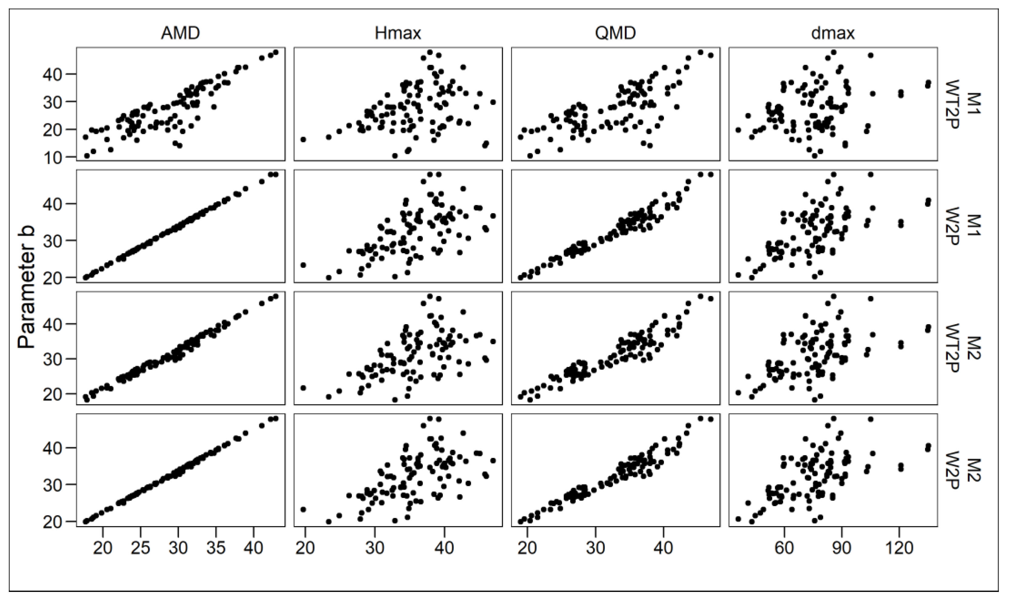
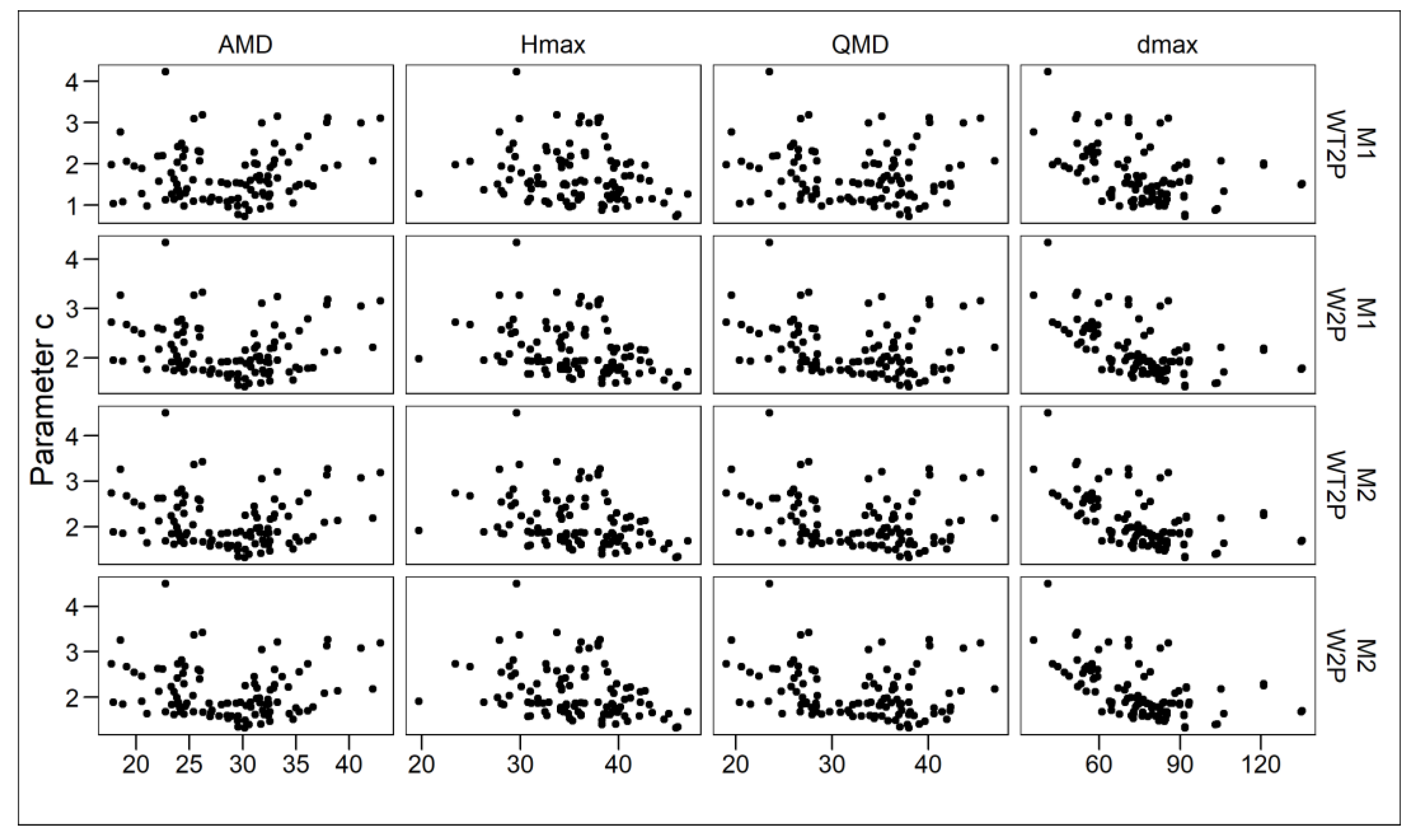
In M1 and M2, the parameters of the W2P and WT2P were estimated for each individual PSP. The stand characteristics were found to explain that the parameters variation are the arithmetic mean diameter (AMD), the quadratic mean diameter (QMD), the maximum height (Hmax), and the maximum diameter (dmax) (Figure 2 and Figure 3). Among the stand characteristics that showed a higher correlation with the estimated parameters are the AMD and QMD.

Even so, AMD was avoided due to its sensitivity to extreme values compared to the QMD but more importantly, it is not usually measured during the forest management planning fieldwork.

Parameter b displays a stronger relationship with the stand characteristics than parameter c (Figure 3). The variation of the WT2P parameter b estimated with M1 through ML is higher than the variation obtained for the same parameter with M2 through the MM.

Other stand characteristics (basal area per hectare, the number of trees per hectare) were tested but none of them or their transformations were found to explain the parameters variation.

The regression models developed for predicting the parameters of the W2P and WT2P are:

$$ln\left(b\right)={\beta }_1+{\beta }_{1}ln\left(QMD\right)$$

(16)

$$ln\left(c\right)={\alpha }_1+{\alpha }_{2}ln\left(QMD\right)+{\alpha }_3\left(\frac{Hmax}{dmax}\right)$$

(17)

where $\beta$ and $\alpha$ are the coefficients of the regression equation (

Table 3. Regression coefficients and standard errors estimated for the parameter prediction method.

Model	Distr.	Term	Estimate	Std. Error
M1	W2P	${\beta }_1$	0.2415	0.0693
M1	W2P	${\beta }_2$	0.9291	0.0200
M1	W2P	${\alpha }_1$	1.3385	0.3408
M1	W2P	${\alpha }_2$	−0.2440	0.0938
M1	W2P	${\alpha }_3$	0.4956	0.1091
M1	WT2P	${\beta }_1$	−0.2694	0.3732
M1	WT2P	${\beta }_2$	1.0211	0.1075
M1	WT2P	${\alpha }_1$	0.1905	0.5916
M1	WT2P	${\alpha }_2$	−0.0229	0.1628
M1	WT2P	${\alpha }_3$	0.7545	0.1899
M2	W2P	${\beta }_1$	0.2450	0.0768
M2	W2P	${\beta }_2$	0.9263	0.0221
M2	W2P	${\alpha }_1$	1.3383	0.3761
M2	W2P	${\alpha }_2$	−0.2556	0.1037
M2	W2P	${\alpha }_3$	0.5311	0.1185
M2	WT2P	${\beta }_1$	0.1124	0.1140
M2	WT2P	${\beta }_2$	0.9536	0.0328
M2	WT2P	${\alpha }_1$	1.4179	0.3777
M2	WT2P	${\alpha }_2$	−0.2685	0.1038
M2	WT2P	${\alpha }_3$	0.4598	0.1225
M3	W2P	${\beta }_1$	0.2429	0.0849
M3	W2P	${\beta }_2$	0.9312	0.0252
M3	W2P	${\alpha }_1$	0.8606	0.1675
M3	W2P	${\alpha }_2$	−0.1888	0.0425
M3	W2P	${\alpha }_3$	1.0347	0.0936
M3	WT2P	${\beta }_1$	−0.2255	0.1440
M3	WT2P	${\beta }_2$	1.0335	0.0420
M3	WT2P	${\alpha }_1$	0.0857	0.2427
M3	WT2P	${\alpha }_2$	−0.0087	0.0653
M3	WT2P	${\alpha }_3$	0.9138	0.1189
M4	W2P	${\beta }_1$	0.2325	0.8149
M4	W2P	${\beta }_2$	0.9338	0.2370
M4	W2P	${\alpha }_1$	0.9504	1.5695
M4	W2P	${\alpha }_2$	−0.2001	0.3981
M4	W2P	${\alpha }_3$	0.9247	0.8650
M4	WT2P	${\beta }_1$	−0.2697	1.4253
M4	WT2P	${\beta }_2$	1.0447	0.4084
M4	WT2P	${\alpha }_1$	0.1271	2.3317
M4	WT2P	${\alpha }_2$	−0.0083	0.6271
M4	WT2P	${\alpha }_3$	0.8087	1.0965

Where M1 to M4 are the four modeling approaches used in the PPM method, Distr column represents the theoretical distribution used, the Term column presents the name of the coefficients, and the Estimate and Std. Error columns present the values of the coefficients and their associated standard errors.

), ln is the natural logarithm, and the other elements were described above.

Logarithm transformation was applied, when necessary, to stabilize the variance of the residuals and improve the model fit. The regression coefficients obtained for the parameter prediction methods are presented in Table 3.

3.2. Parameter Recovery Method

In order to recover the parameters of the W2P and WT2P distribution using the MM, the AMD was predicted using Equation (18) fitted with the ordinary least squares method.

$$AMD=QMD-\exp \left(a_0+a_{1}G+a_{3}N\right)$$

(18)

where, $a_0$, $a_1\mathrm{and}{a}_2$ are regression coefficients presented in

Table 4. Estimated regression coefficients and fitting performance.

Coefficients Estimates					Fitting Statistics
Term	Estimate	Std. Error	t-Value	p-Value	RMSE	Bias
$a_0$	1.7607	0.2063	8.534	0.0000	1.2840	−0.006
$a_1$	0.0056	0.0025	2.202	0.0299
$a_2$	−0.0010	0.0001	−5.882	0.0000

All coefficients are significant at 0.05 level. The RMSE value is only 1.284 and the model is basically unbiased.

, G is the basal area per hectare, N is the number of trees per hectare, and the other elements are described above. The independent variables were chosen so their t-values are higher than 2.

3.3. Fitting Performance of the Methods and Models on the Fitting Dataset

The theoretical distribution that predicted the number of trees and the sum of diameters with the highest accuracy was the WT2P (

Table 5. Evaluation of the considered methods and functions applied to the fitting dataset.

Method.	Model	Distr.	%RMSE				%Bias				Score	Rank
			d0	d1	d2	d3	d0	d1	d2	d3
PPM	M1	W2P	0.00	6.42	4.22	9.42	0.00	−4.55	−3.28	1.88	21.96	5
				(5.09)	(3.53)	(1.08)		(7.43)	(3.23)	(1.59)
PPM	M1	WT2P	0.00	8.65	14.96	21.97	0.00	6.21	13.19	18.44	60.00	10
				(10)	(10)	(10)		(10)	(10)	(10)
PPM	M2	W2P	0.00	6.31	4.48	9.31	0.00	−4.34	−3.44	0.72	20.99	4
				(4.85)	(3.69)	(1.00)		(7.11)	(3.34)	(1.00)
PPM	M2	WT2P	0.00	4.56	4.44	15.68	0.00	−0.91	3.69	11.98	22.23	6
				(1.00)	(3.67)	(5.53)		(1.80)	(3.51)	(6.72)
PPM	M3	W2P	0.00	7.41	8.05	11.90	0.00	−5.62	−6.37	−4.46	33.31	8
				(7.28)	(5.84)	(2.84)		(9.10)	(5.34)	(2.90)
PPM	M3	WT2P	0.00	5.53	6.76	13.42	0.00	−0.39	−1.16	−3.85	17.50	2
				(3.13)	(5.06)	(3.93)		(1.00)	(1.78)	(2.59)
PPM	M4	W2P	0.00	7.56	8.57	12.76	0.00	−5.74	−6.57	−4.78	35.03	9
				(7.61)	(6.15)	(3.45)		(9.28)	(5.48)	(3.06)
PPM	M4	WT2P	0.00	5.72	7.60	14.72	0.00	−0.63	−1.47	−4.18	20.08	3
				(3.55)	(5.57)	(4.85)		(1.36)	(2.00)	(2.76)
PRM	M5	W2P	0.00	6.85	6.18	11.26	0.00	−5.46	−6.13	−3.89	29.76	7
				(6.03)	(4.71)	(2.39)		(8.84)	(5.18)	(2.61)
PRM	M5	WT2P	0.00	4.84	0.02	12.57	0.00	−2.41	0.01	5.50	14.48	1
				(1.60)	(1.00)	(3.32)		(4.12)	(1.00)	(3.42)

The relative rank is presented in parenthesis. The sum of the relative ranks is found in the column named Score while the ranking obtained by each method and function is displayed in the column named Rank. The d⁰ to d³ represent the power the diameters were raised to.

). The first three places in the ranking were occupied by the WT2P, while the best ranking obtained by W2P was the fourth one. Even so, overall, W2P tended to have higher accuracy than WT2P when the sums of the diameters were raised to the second and third powers.

The modeling approaches used showed a clear difference between the classic two-stage PPM (M1, M2) and the simultaneous fitting approach (M3, M4). Nevertheless, the parameters that estimate with the highest accuracy of the experimental distribution were obtained with the PRM using the method of moments. The accuracy obtained by WT2P through M5 measured by the %RMSE statistic was rather small with only 4.8% for the sum of the diameters, up to 12.6% to the sums of the third powers of diameters that approximate the volume of the stand and only 0.02% for the sums of the second powers of diameters that approximate the basal area of the stand. The values of %Bias statistic was between 2.4% and 5.5% with the lowest value registered by the sums of the second powers of diameters (0.01%). The M3 modeling approach was very similar to the M4 modeling approach, the difference between them being the weighted sum of plot-specific log-likelihoods applied in M3 which increased the accuracy of the model. Both models performed well ranking in second and third place using the WT2P. The worst performance was registered by the WT2P in the modeling approach M1 which ranked last in every evaluation criterion, reaching an imprecision up to 22% for the sums of the third powers of diameters.

3.4. Fitting Performance of the Methods and Models on the Test Dataset

The dataset used to test the methods and models developed had a plot size area between 0.25 and 1 ha which captured better the distribution of the forest stand where these plots had been installed than the PSPs used to obtain the models’ coefficients. The PRM method using the WT2P distribution (M5) ranked again first (

Table 6. Evaluation of the considered methods and functions applied to the test dataset.

Method.	Model	Distr.	%RMSE				%Bias				Score	Rank
			d0	d1	d2	d3	d0	d1	d2	d3
PPM	M1	W2P	0.00	5.58	3.81	6.90	0.00	−3.40	−3.05	−1.91	17.09	2
				(3.46)	(3.19)	(1.00)		(4.71)	(3.00)	(1.72)
PPM	M1	WT2P	0.00	(9.68)	(15.58)	(17.04)	0.00	7.88	13.68	13.88	60.00	10
				(10)	(10)	(10)		(10)	(10)	(10
PPM	M2	W2P	0.00	5.49	4.15	7.62	0.00	−3.19	−3.36	−3.47	18.80	4
				(3.31)	(3.39)	(1.64)		(4.46)	(3.20)	(2.80)
PPM	M2	WT2P	0.00	4.16	4.52	10.20	0.00	0.25	3.62	6.98	18.33	3
				(1.19)	(3.60)	(3.93)		(1.00)	(3.38)	(5.23)
PPM	M3	W2P	0.00	6.74	8.22	13.08	0.00	−4.79	−7.00	−9.65	36.58	9
				(5.32)	(5.74)	(6.49)		(6.36)	(5.60)	(7.07)
PPM	M3	WT2P	0.00	5.26	6.90	14.39	0.00	0.29	−2.34	−9.68	26.25	6
				(2.95)	(4.98)	(7.65)		(1.04)	(2.53)	(7.10)
PPM	M4	W2P	0.00	6.60	7.79	12.46	0.00	−4.68	−6.78	−9.30	35.04	8
				(5.09)	(5.50)	(5.94)		(6.22)	(5.46)	(6.83)
PPM	M4	WT2P	0.00	5.11	6.19	13.53	0.00	0.51	−2.02	−9.32	24.65	5
				(2.72)	(4.57)	(6.89)		(1.31)	(2.32)	(6.85)
PRM	M5	W2P	0.00	6.00	6.86	12.04	0.00	−4.38	−6.72	−8.58	32.27	7
				(4.14)	(4.96)	(5.56)		(5.87)	(5.41)	(6.33)
PRM	M5	WT2P	0.00	4.04	0.02	8.86	0.00	−0.88	−0.02	0.87	8.49	1
				(1.00)	(1.00)	(2.74)		(1.75)	(1.00)	(1.00)

The relative rank is presented in parenthesis. The sum of the relative ranks is found in the column named Score while the score obtained by each method and function is ranked in the column named Rank. The d⁰ to d³ represent the power the diameters were raised to.

). For this modeling approach, the results were comparable with the ones obtained for the fitting dataset. Furthermore, the %Bias values registered using this modeling approach were smaller than the ones obtained for the fitting dataset. The M5 model performed the best in predicting the sums of the second powers of the diameters while the worst performance was in predicting the values of the sums of the third powers of the diameters. Although M3 and M4 ranked second and third when fitting the fitting dataset, their performance was rather poor on the test dataset. Their ranking was 6th and 5th, higher than M1 and M2. The W2P best-ranking was obtained using the M1 method, while the WT2P using the same method ranked again last at every criterion used. The score obtained by the model ranked second was double the one obtained by the model that ranked first, while the third and the fourth obtained similar scores. W2P tended to achieve lower %RMSE and %Bias values at higher powers (d² and d³) while WT2P behaved better when predicting the sum of diameters (d¹).

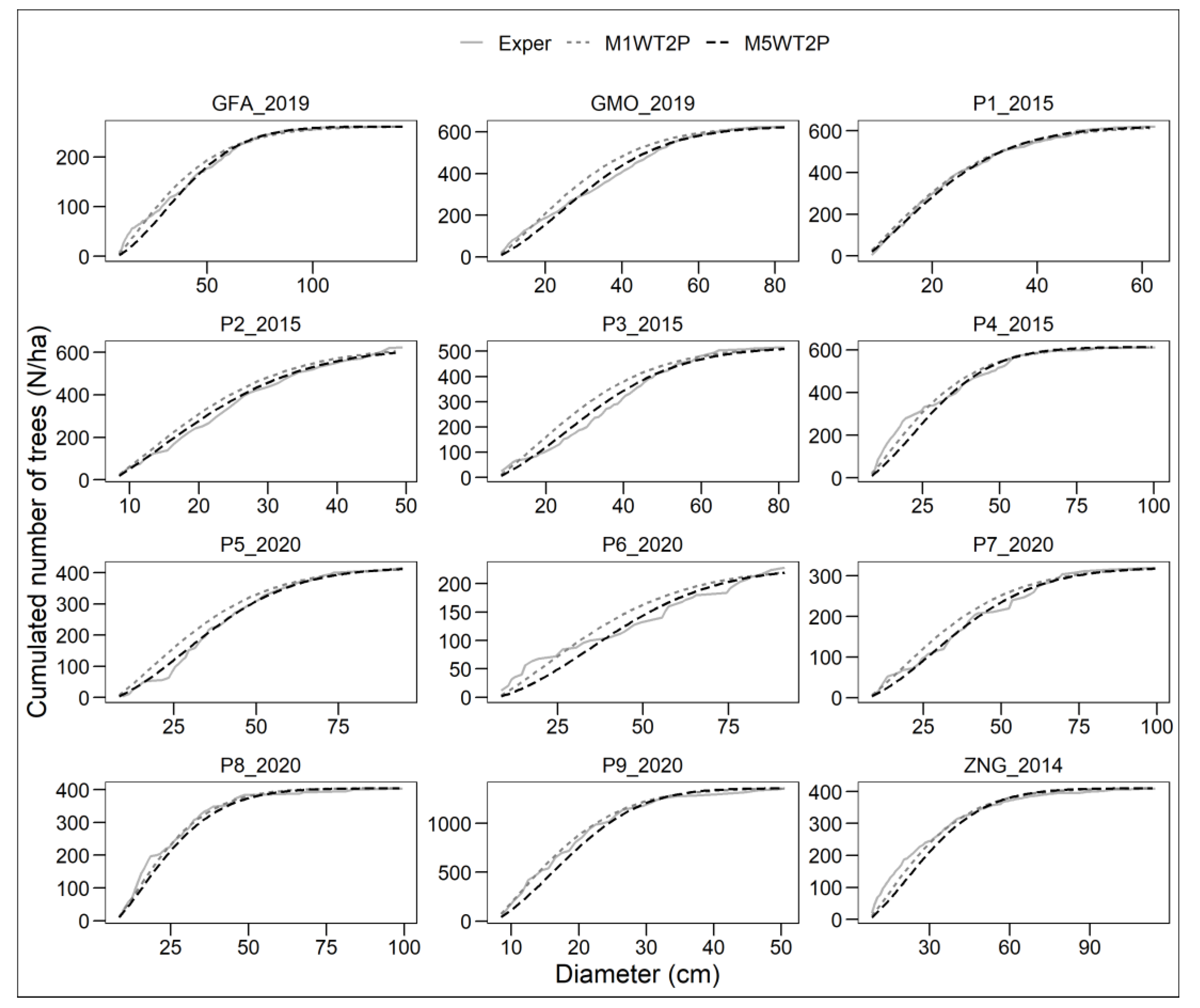
The estimation of 12 out of 17 diameter distributions used in the test dataset is graphically displayed below (Figure 4). The M5 and M3 modeling approach using the WT2P which performed best in all cases was used to illustrate the fitting achieved for these plots. In most cases, the models underestimated the number of trees in the first diameters categories. Even so, the overall shape of the fitting was similar to one of the experimental distributions.

4. Discussion

Prediction of the diameter distribution is usually needed in forest management planning and forest growth simulators where inventory data is not available. Weibull distribution (WD) has been widely applied to such modeling tasks, especially in even-aged pure stands [12,37,38,39]. However, due to its capacity to take various shapes and produce a good fit in heterogenous pine stands [40], mixed uneven-aged pine-dominated stands [41], or uneven-aged pine-oak mixed forests [20], the Weibull function was chosen to apply the parameter prediction and parameter recovery methods. There are several formulations of the Weibull distribution function in the literature [24], yet there is no unified agreement on which formulation is more suitable for describing the diameter distribution. Although the 3-parameter Weibull (3W) formulation is considered more flexible [8], other valid criteria for choosing the right model should also include parsimony (i.e., the lowest possible number of parameters) and logical interpretation.

Several comparative studies found that the 2-parameter Weibull (2W) formulation performs better than the 3W formulation. For example, Maltamo et al. [9] argued that removing the location parameter allowed the frequency values to rapidly increase above zero which is preferred, especially in uneven-aged stands. Schmidt et al. [12] evaluated all eight Weibull formulations and found that the right truncated 2W formulation performed better than all other formulations including the 3W ones. Taking into account previous research papers as well as the one presented above, the parsimony of the model, and that rationally the function should start from 0, we found the 2W formulation better suited for modeling the diameter distribution in uneven-aged stands than 3W formulation.

In Romania, Weibull distribution was tested before [42] against the Gamma and the Normal distribution in 12 pure and mixed plots of both even and uneven-aged structures of 1-ha size and performed very well in almost all cases. In contrast to our modeling approach, Horodnic and Roibu [43] used a Gaussian multi-component model to fit the experimental distribution of a natural silver fir-beech mixed old-growth forest stand from Şinca Veche (Făgăraş Mountains, Romania). This method involves splitting the stand into homogeneous age groups and applying the normal distribution for each of the groups. By summing the Gaussian probability density function of each age group, the cumulative distribution is obtained. This method proved to be more precise than the negative exponential distribution applied by Meyer [18] and used in Romania by Popescu-Zeletin and Dissescu [44] to develop diameter distribution models for spruce-silver fir-beech uneven-aged stands. A similar approach was conducted by Chivulescu et al. [45], who used a mixture of three normal distributions to describe the stand structure of the Penteleu-Viforâta virgin forest in the Curvature Carpathians, Romania. Nevertheless, these methods can hardly be applied to predict the diameter distribution of a new stand based on basic stand characteristics. In fact, the parameter prediction and parameter recovery methods have not been applied in Romania until now. Furthermore, the application of the left-truncated 2 parameters Weibull distribution (WT2P) for forest inventory data has not been tested yet either.

The WT2P achieved a better prediction for even and uneven-aged stands in Catalonia compared to the complete 2 parameters Weibull (W2P), beta, and Johnson’s SB distribution [10]. A similar finding is obtained through our research too, where WT2P had the highest accuracy in predicting the diameter distribution and the sums of the diameters raised to the first, second, and third powers. The results are consistent with the ones presented in previous studies [10,19,24] which underlined that the use of the complete W2P to censored data should be avoided, otherwise a systematic error in the parameters is inserted. In contrast to our findings, the research of Schmidt et al. [12] conducted in clonal eucalypt stands, found that the right-truncated two-parameter formulation performed better than seven other different formulations of the WD (including the WT2P formulation). In our case, the predicted maximum diameter is directly linked to the shape parameter which with the PPM, is predicted using the measured maximum diameter and maximum height. Although WT2P finds its justification for forest inventory data [19,24,25,33] which is censored from a certain diameter due to practical reasons, in our opinion, the right truncation WD has low applicability in uneven-aged stands where one hardly measures the real maximum diameter of the stand but rather only estimates it based on the sample plot inventoried, as it was in our case. An unnecessary right censoring can lead to a seriously biased stand volume underestimation. A right truncation should be made with caution if only the real maximum diameter of the stand was measured. The maximum diameter and maximum height ratio used to predict the parameter c of the functions is a measure of stand density, age, and climate [46]. The distribution will have a negative exponential shape if the ratio between the maximum height and diameter is close to 0. This is a logical behavior as the presence of large trees with a reduced height is a characteristic of the initial and optimum development stages which are characterized by a large number of trees in lower diameter classes [47]. Although dominant or mean height is usually used to predict or recover the parameters of the diameter distribution for even-aged stands [48], dominant height models are not applicable to uneven-aged stands. The maximum height is a stand characteristic that is more stable and easier to measure than the mean height. In addition, an approximation of the maximum height can be estimated using airborne laser scanning data and used to predict the parameter [49]. If unavailable, this measurement is not necessary and the parameter of the WT2P can be predicted using the equation developed to predict the arithmetic mean diameter for the MM. The PRM based on the MM was found to perform better than all PPM modeling approaches. Our findings are similar to Cao’s [32], the simultaneous fitting based on method 6 described in his research paper had the highest accuracy of all modeling approaches applied in the PPM outperforming the three steps approach. Even so, the PRM method based on MM provided consistent results for both the fitting and the test dataset. The MM is acknowledged by some authors as the most accurate method for estimating WD parameters [19,37,50,51]. This method also gave the best results in uneven-aged pine-oak mixed forests in the Qinling Mountains of China [20], a forest with a similar structure to ours. MM has the advantage of obtaining the parameters based only on the mean diameter and the quadratic mean diameter. Furthermore, the PRM assures that the estimated parameters are directly linked with the first and second raw moments of the experimental distribution. The accuracy of this method is secured by ensuring the inequalities between the arithmetic mean diameter and the quadratic mean diameter $\left(AMD<QMD\right)$ [48]. This inequality is fulfilled by the equation formulated to predict the arithmetic mean diameter. The PRM outperformed all other modeling approaches used in predicting the sums of the second powers of diameters that approximate the basal area of the stand. Nevertheless, similar results to ours were obtained by previous studies. For example, in Palahí et al. [10], the WT2P %RMSE’s values reached up to 12.9 % for the sums of diameters of the third power. Maltamo et al. [9] obtained a %RMSE’ of only 5.4% for the W2P while the results obtained in this research for the modeling approach that ranked first is 12.6% and 8.9% for the fitting and the test dataset respectively.

Uneven-aged forests are characterized by a high structural diversity with tree saplings and trees at their longevity limit, growing together on the same patch of the stand. This is possible due to species niche complementarity and reduced light requirements of the species in the mixture. Furthermore, uneven-aged forests are known for their stability and productivity, and they are considered a tool for climate change mitigation [52,53,54].

This work is particularly important as these types of forests are increasingly rare. Mixed conifer uneven-aged forests were previously exploited in most countries and replaced by spruce monocultures [55] due to their high productivity and fine wood quality. Patches that remained untouched are increasingly rare and disperse across Europe. Most of the forests from the study area are virgin forests or have not been touched for more than 60 years ago. Their present image is shaped only by the legacy of previous natural events, competition, and mortality. These forests are an important resource for silvicultural practices in understanding what are the natural dynamics that allow them to obtain the stability they are known to possess.

This is a particularly important feature of this research and as far as we know, there are no previous research papers that focused solely on mixed unmanaged uneven-aged stands. The equations developed in this research cannot only serve to accurately predict the diameter distribution but also serve as a conversion regime for even-aged mixed forests to uneven-aged forests. The shift from even-aged to uneven-aged can be achieved by using such tools that can aid first managers to apply the necessary silvicultural treatments. Using basic stand characteristics, forests managers can develop a reference diameter distribution that can serve as a management guide for obtaining uneven-aged structures. Similar to the q-factor method promoted by Meyer [18] to obtain balanced uneven age stands, the equations developed in this research can also be used to create a negative exponential distribution or rotate-sigmoid which are more commonly accepted as stand balanced structures [56,57,58].

Nowadays, forest research and practice tend to migrate the silvicultural practices to emulate the natural development of uneven-aged forests [59]. In order to obtain such a diverse structure, yield and growth models are needed to simulate the stand dynamics as a result of the silvicultural practices applied [60]. Diameter distribution prediction is one of the main outputs of a growth model.

5. Conclusions

This research is one of the limited attempts to predict the diameter distribution in unmanaged uneven-aged stands and the first of this kind in Romania. However, the equations developed in this research can serve as a common tool for creating reference distributions of uneven-aged stands in similar forests and conditions to ours all across Europe. Furthermore, the application of these methods is beneficial both to the Retezat National Park administration where this study was conducted and to Romanian forest management planning overall. The Park administration will be able to assess accurately and more easily the size and structure of their forest resources. For the management planning, this can serve as an example that the parameter prediction and parameter recovery methodology presented in this paper should be an alternative solution to avoid the limitations of yield tables when estimating the volume of mixed-species uneven-aged stands.

References

- MacDicken, K.G. Global Forest Resources Assessment 2015: What, why and how? For. Ecol. Manage. 2015. [Google Scholar] [CrossRef] [Green Version]
- Helms, J.A. The Dictionary of Forestry; Society of American Foresters: Bethesda, MD, USA, 1998; p. 210. ISBN 0-85199-308-7. [Google Scholar]
- Hummel, S.; O’Hara, K.L. Forest Management. In Ecological Engineering; Jørgensen, S.E., Fath, B.D.B.T.E., Eds.; Academic Press: Oxford, UK, 2008; Volume 2, pp. 1653–1662. ISBN 978-0-08-045405-4. [Google Scholar]
- Kuuluvainen, T.; Penttinen, A.; Leinonen, K.; Nygren, M. Statistical opportunities for comparing stand structural heterogeneity in managed and primeval forests: An example from boreal spruce forest in southern Finland. Silva Fenn. 1996. [Google Scholar] [CrossRef] [Green Version]
- Clutter, J.L.; Bennett, F.A. Diameter distribution in old-field slash pine plantations. GA. For. Res. Counc. Rep 1965, 13, 9. [Google Scholar]
- Hyink, D.M.; Moser, J.W., Jr. A Generalized Framework for Projecting Forest Yield and Stand Structure Using Diameter Distributions. For. Sci. 1983, 29, 85–95. [Google Scholar]
- Cajanus, W. Ueber die Entwicklung gleichaltriger Waldbestande: Eine statistische Studie. Acta For. Fenn. 1914, 3, 142. [Google Scholar] [CrossRef]
- Bailey, R.; Dell, T. Quantifying Diameter Distributions with the Weibull Function. For. Sci. 1973. [Google Scholar] [CrossRef]
- Maltamo, M.; Puumalainen, J.; Päivinen, R. Comparison of beta and Weibull functions for modelling basal area diameter distribution in stands of Pinus sylvestris and Picea abies. Scand. J. For. Res. 1995, 10, 284–295. [Google Scholar] [CrossRef]
- Palahí, M.; Pukkala, T.; Blasco, E.; Trasobares, A. Comparison of beta, Johnson’s SB, Weibull and truncated Weibull functions for modeling the diameter distribution of forest stands in Catalonia (north-east of Spain). Eur. J. For. Res. 2007. [Google Scholar] [CrossRef]
- Podlaski, R. Forest modelling: The gamma shape mixture model and simulation of tree diameter distributions. Ann. For. Sci. 2017. [Google Scholar] [CrossRef] [Green Version]
- Schmidt, L.N.; Sanquetta, M.N.I.; McTague, J.P.; da Silva, G.F.; Fraga Filho, C.V.; Sanquetta, C.R.; Soares Scolforo, J.R. On the use of the weibull distribution in modeling and describing diameter distributions of clonal eucalypt stands. Can. J. For. Res. 2020. [Google Scholar] [CrossRef]
- Schiffel, A. Wuchsgesetze Normaler Fichtenbenbestande; Mitt Forstl Versuchswesen Osterreichs. Heft XXIX; 1904. [Google Scholar]
- Borders, B.E.; Souter, R.A.; Bailey, R.L.; Ware, K.D. Percentile-based distributions characterize forest stand tables. For. Sci. 1987, 33, 570–576. [Google Scholar]
- Maltamo, M.; Kangas, A. Methods based on k-nearest neighbor regression in the prediction of basal area diameter distribution. Can. J. For. Res. 1998. [Google Scholar] [CrossRef]
- Reis, L.P.; de Souza, A.L.; Mazzei, L.; dos Reis, P.C.M.; Leite, H.G.; Soares, C.P.B.; Torres, C.M.M.E.; da Silva, L.F.; Ruschel, A.R. Prognosis on the diameter of individual trees on the eastern region of the amazon using artificial neural networks. For. Ecol. Manage. 2016. [Google Scholar] [CrossRef]
- Liocourt, F. de De l’aménagement des sapinières. Bull. la Société For. Fr. Belfort 1898, 6, 396–405. [Google Scholar]
- Meyer, H.A. Structure, Growth, and Drain in Balanced Uneven-Aged Forests. J. For. 1951, 50, 85–92. [Google Scholar]
- Merganič, J.; Sterba, H. Characterisation of diameter distribution using the Weibull function: Method of moments. Eur. J. For. Res. 2006. [Google Scholar] [CrossRef]
- Sun, S.; Cao, Q.V.; Cao, T. Characterizing diameter distributions for uneven-aged pine-oak mixed forests in the Qinling Mountains of China. Forests 2019, 10, 596. [Google Scholar] [CrossRef] [Green Version]
- Pretzsch, H. Konzeption und konstruktion von wuchsmodellen fur rein-und mischbestande. Forstl Forschungsberichte München 1992, 115, 115–358. [Google Scholar]
- Pretzsch, H.; Biber, P.; Ďurský, J. The single tree-based stand simulator SILVA: Construction, application and evaluation. For. Ecol. Manage. 2002. [Google Scholar] [CrossRef]
- Nagel, J. BWERT: Programm zur Bestandesbewertung und zur Prognose der Bestandesentwicklung. DFFA, Sekt. Ertragskunde, Jahrestagung Joachimsthal 1995, 166, 185–189. [Google Scholar]
- Zutter, B.R.; Oderwald, R.G.; Murphy, P.A.; Farrar, R.M. Characterizing diameter distributions with modified data types and forms of the Weibull distribution. For. Sci. 1986. [Google Scholar] [CrossRef]
- Palahí, M.; Pukkala, T.; Trasobares, A. Modelling the diameter distribution of Pinus sylvestris, Pinus nigra and Pinus halepensis forest stands in Catalonia using the truncated Weibull function. Forestry 2006. [Google Scholar] [CrossRef] [Green Version]
- Ciceu, A.; Garcia-Duro, J.; Seceleanu, I.; Badea, O. A generalized nonlinear mixed-effects height–diameter model for Norway spruce in mixed-uneven aged stands. For. Ecol. Manage. 2020. [Google Scholar] [CrossRef]
- Bankston, J.B.; Sabatia, C.O.; Poudel, K.P. Effects of Sample Plot Size and Prediction Models on Diameter Distribution Recovery. For. Sci. 2021. [Google Scholar] [CrossRef]
- Robinson, A. Preserving correlation while modelling diameter distributions. Can. J. For. Res. 2004. [Google Scholar] [CrossRef]
- Team, C. R: A Language and Environment for Statistical Computing; R Foundation for Statistical Computing: Vienna, Austria, 2020. [Google Scholar]
- Mehtätalo, L.; Lappi, J. Biometry for Forestry and Environmental Data: With Examples in R; Chapman and Hall; CRC Press: New York, NY, USA, 2020; p. 426. [Google Scholar]
- Zellner, A. An Efficient Method of Estimating Seemingly Unrelated Regressions and Tests for Aggregation Bias. J. Am. Stat. Assoc. 1962. [Google Scholar] [CrossRef]
- Cao, Q.V. Predicting parameters of a weibull function for modeling diameter distribution. For. Sci. 2004. [Google Scholar] [CrossRef]
- Räty, J.; Astrup, R.; Breidenbach, J. Prediction and model-assisted estimation of diameter distributions using Norwegian national forest inventory and airborne laser scanning data. Can. J. For. Res. 2021. [Google Scholar] [CrossRef]
- Bitterlich, W. Die Winkelzählprobe. Forstwissenschaftliches Cent. 1952. [Google Scholar] [CrossRef]
- Stoyan, D.; Penttinen, A. Recent applications of point process methods in forestry statistics. Stat. Sci. 2000. [Google Scholar] [CrossRef]
- Hadley, W. ggplot2: Elegant Graphics for Data Analysis; Springer: New York, NY, USA, 2016. [Google Scholar]
- Lei, Y. Evaluation of three methods for estimating the Weibull distribution parameters of Chinese pine (Pinus tabulaeformis). J. For. Sci. 2008. [Google Scholar] [CrossRef] [Green Version]
- Schütz, J.P.; Rosset, C. Performances of different methods of estimating the diameter distribution based on simple stand structure variables in monospecific regular temperate European forests. Ann. For. Sci. 2020. [Google Scholar] [CrossRef]
- Rennolls, K.; Geary, D.N.; Rollinson, T.J.D. Characterizing diameter distributions by the use of the weibull distribution. Forestry 1985. [Google Scholar] [CrossRef]
- Maltamo, M.; Kangas, A.; Uuttera, J.; Torniainen, T.; Saramäki, J. Comparison of percentile based prediction methods and the Weibull distribution in describing the diameter distribution of heterogeneous Scots pine stands. For. Ecol. Manage. 2000. [Google Scholar] [CrossRef]
- Návar, J.; Corral, S. Estimating, predicting and recovering Weibull distribution parameters of mixed and uneven-aged stands of Durango, Mexico. In Forest Ecosystem Restoration: Ecological and Economical Impacts of Restoration Processes in Secondary Coniferous Rorests, Proceedings of the International Conference, Vienna, Austria, 10–12 April 2000; Institute of Forest Growth Research: Wien, Austria, 2000; pp. 187–193. [Google Scholar]
- Leca, Ș.; Dumitru, I.; Silaghi, D.; Chivulescu, Ș. Tree diameter distribution in the Romanian extended intensive monitoring network (Level II). Rev. Pădurilor 2014, 129, 3–11. [Google Scholar]
- Horodnic, S.A.; Roibu, C.C. A Gaussian multi-component model for the tree diameter distribution in old-growth forests. Eur. J. For. Res. 2018. [Google Scholar] [CrossRef]
- Popescu-Zeletin, I.; Dissescu, R. Caracterizarea și clasificarea după structură a arboretelor pluriene din Carpații R.S.R. Bul. Stiințific. Acad. R.S.R. 1966, 1, 67–77. [Google Scholar]
- Chivulescu, S.; Ciceu, A.; Leca, S.; Apostol, B.; Popescu, O.; Badea, O. Development phases and structural characteristics of the Penteleu-Viforâta virgin forest in the Curvature Carpathians. iForest-Biogeosciences For. 2020, 13, 389. [Google Scholar] [CrossRef]
- Zhang, X.; Wang, H.; Chhin, S.; Zhang, J. Effects of competition, age and climate on tree slenderness of Chinese fir plantations in southern China. For. Ecol. Manage. 2020. [Google Scholar] [CrossRef]
- Feldmann, E.; Glatthorn, J.; Hauck, M.; Leuschner, C. A novel empirical approach for determining the extension of forest development stages in temperate old-growth forests. Eur. J. For. Res. 2018, 137(3), 321–335. [Google Scholar] [CrossRef]
- Siipilehto, J.; Mehtätalo, L. Parameter recovery vs. parameter prediction for the Weibull distribution validated for Scots pine stands in Finland. Silva Fenn. 2013. [Google Scholar] [CrossRef]
- Gobakken, T.; Næsset, E. Estimation of diameter and basal area distributions in coniferous forest by means of airborne laser scanner data. Scand. J. For. Res. 2004, 19, 529–542. [Google Scholar] [CrossRef]
- Nanang, D.M. Suitability of the Normal, Log-normal and Weibull distributions for fitting diameter distributions of neem plantations in Northern Ghana. For. Ecol. Manage. 1998. [Google Scholar] [CrossRef]
- Pobočíková, I.; Sedliačková, Z. Comparison of four methods for estimating the Weibull distribution parameters. Appl. Math. Sci. 2014. [Google Scholar] [CrossRef]
- Hilmers, T.; Avdagi, A.; Bartkowicz, L.; Bielak, K.; Binder, F.; Bonina, A.; Dobor, L.; Forrester, D.I.; Hobi, M.L.; Ibrahimspahi, A.; et al. The productivity of mixed mountain forests comprised of Fagus sylvatica, Picea abies, and Abies alba across Europe. Forestry 2020. [Google Scholar] [CrossRef] [Green Version]
- Nikolova, P.S.; Raspe, S.; Andersen, C.P.; Mainiero, R.; Blaschke, H.; Matyssek, R.; Häberle, K.H. Effects of the extreme drought in 2003 on soil respiration in a mixed forest. Eur. J. For. Res. 2009. [Google Scholar] [CrossRef]
- Pretzsch, H.; Block, J.; Dieler, J.; Dong, P.H.; Kohnle, U.; Nagel, J.; Spellmann, H.; Zingg, A. Comparison between the productivity of pure and mixed stands of Norway spruce and European beech along an ecological gradient. Ann. For. Sci. 2010. [Google Scholar] [CrossRef] [Green Version]
- Seidl, R.; Rammer, W.; Jäger, D.; Currie, W.S.; Lexer, M.J. Assessing trade-offs between carbon sequestration and timber production within a framework of multi-purpose forestry in Austria. For. Ecol. Manage. 2007. [Google Scholar] [CrossRef]
- West, D. Canopy-understory Interaction Effects on Forest Population Structure. For. Sci. 1975. [Google Scholar] [CrossRef]
- Janowiak, M.K.; Nagel, L.M.; Webster, C.R. Spatial Scale and Stand Structure in Northern Hardwood Forests: Implications for Quantifying Diameter Distributions. For. Sci. 2008. [Google Scholar] [CrossRef]
- Alessandrini, A.; Biondi, F.; Di Filippo, A.; Ziaco, E.; Piovesan, G. Tree size distribution at increasing spatial scales converges to the rotated sigmoid curve in two old-growth beech stands of the Italian Apennines. For. Ecol. Manage. 2011. [Google Scholar] [CrossRef]
- Schneider, R.; Franceschini, T.; Duchateau, E.; Bérubé-Deschênes, A.; Dupont-Leduc, L.; Proudfoot, S.; Power, H.; de Coligny, F. Influencing plantation stand structure through close-to-nature silviculture. Eur. J. For. Res. 2021. [Google Scholar] [CrossRef]
- Hamidi, S.K.; Weiskittel, A.; Bayat, M.; Fallah, A. Development of individual tree growth and yield model across multiple contrasting species using nonparametric and parametric methods in the Hyrcanian forests of northern Iran. Eur. J. For. Res. 2021. [Google Scholar] [CrossRef]
Figure 1.
The sampling design of the permanent sampling plots (PSP).
Figure 2.
Parameter b variation in relation to stand characteristics. AMD, QMD, and dmax x-axis are in cm while Hmax x-axis is in m.
Figure 3.
Parameter c variation in relation to stand characteristics. AMD, QMD, and dmax x-axis are in cm while Hmax x-axis is in m.
Figure 4.
Example of the fitted distribution for 12 plots of the test dataset. Here the Exper represents the experimental distribution, M1WT2P is the M1 modeling approach using the left-truncated Weibull distribution (WT2P), which achieved the last ranking position for both the fitting and the test dataset; M5WT2P is the M5 modeling approach using the left-truncated Weibull distribution (WT2P) which ranked first for both the fitting and the test dataset.