21st Century Planning Techniques for Creating Fire-Resilient Forests in the American West

Abstract

Data-driven decision making is the key to providing effective and efficient wildfire protection and sustainable use of natural resources. Due to the complexity of natural systems, management decision(s) require clear justification based on substantial amounts of information that are both accurate and precise at various spatial scales. To build information and incorporate it into decision making, new analytical frameworks are required that incorporate innovative computational, spatial, statistical, and machine-learning concepts with field data and expert knowledge in a manner that is easily digestible by natural resource managers and practitioners. We prototyped such an approach using function modeling and batch processing to describe wildfire risk and the condition and costs associated with implementing multiple prescriptions for risk mitigation in the Blue Mountains of Oregon, USA. Three key aspects of our approach included: (1) spatially quantifying existing fuel conditions using field plots and Sentinel 2 remotely sensed imagery; (2) spatially defining the desired future conditions with regards to fuel objectives; and (3) developing a cost/revenue assessment (CRA). Each of these components resulted in spatially explicit surfaces describing fuels, treatments, wildfire risk, costs of implementation, projected revenues associated with the removal of tree volume and biomass, and associated estimates of model error. From those spatially explicit surfaces, practitioners gain unique insights into tradeoffs among various described prescriptions and can further weigh those tradeoffs against financial and logistical constraints. These types of datasets, procedures, and comparisons provide managers with the information needed to identify, optimize, and justify prescriptions across the landscape.

1. Introduction

Wildfires are increasing in frequency [1], cost [2,3], and impact [4]. While this increase can be attributed to many factors such as a warming climate [5], recreation [6], increased number of severe events [7], and various anthropogenic-related activities [8], the focus, with regards to the impact of fire, tends to revolve around anthropogenic impacts. Most recently, we have witnessed those consequences in terms of life, property, and social unrest [9], which in turn has helped to focus the wildfire discussions around efficient and effective wildfire protection [10].

Novel approaches to framing wildfire protection (e.g., potential operational delineations) [11] and advancements in physically based modeling tools [12] have been critical to improving our understanding of fire and its potential impacts. Additionally, the successful use of those tools requires data that are accurate at fine resolution, spatially explicit, and current. However, such data often do not exist or are extremely time intensive and costly to develop [13,14]. Moreover, much of the information generated from various existing fire models can be difficult to translate to other metrics related to managing natural resources. In large part, these two limitations, fine resolution, accurate data, and the ability to translate information across fields, significantly reduce wildfire suppression efficiencies and our ability to effectively protect against the impact of wildfire.

Due to the catastrophic nature of some wildfires [9], fire is typically discussed within a negative context as it relates to the impact on natural resources. While there are many examples that highlight the negative impact of fire, the use of fire to manage forests is natural, efficient, has a low cost of implementation, and can be used to control fuel loads [15], all of which can be advantageously used in a controlled and timely manner to meet various objectives across the landscape [16,17]. Here again, the ability to effectively and efficiently use fire is predicated on the knowledge of key metrics such as fuel loads, moisture content, winds, temperature, and topography at high fidelity in both space and time.

This relationship between knowing information at fine resolution and informed decision making is an ever-evolving topic that has received increased attention due to the many advancements in technology and computer science [18]. However, the practical application of those advancements with regards to policy and moving data-driven decision making to the forefront of wildfire management, appears to be lagging behind other fields such as banking, information technology, and telecommunications [19,20]. The slow adoption of data-driven decision making can be attributed, in part, to traditional mandates and classical tactics within the wildfire management community [21]. However, an equally likely aspect to limited adoption of data-driven decision making stems from the lack of computational tools developed for managers that can be used to easily and quickly automate complex modeling techniques and create the fundamental datasets needed to translate information into decisions.

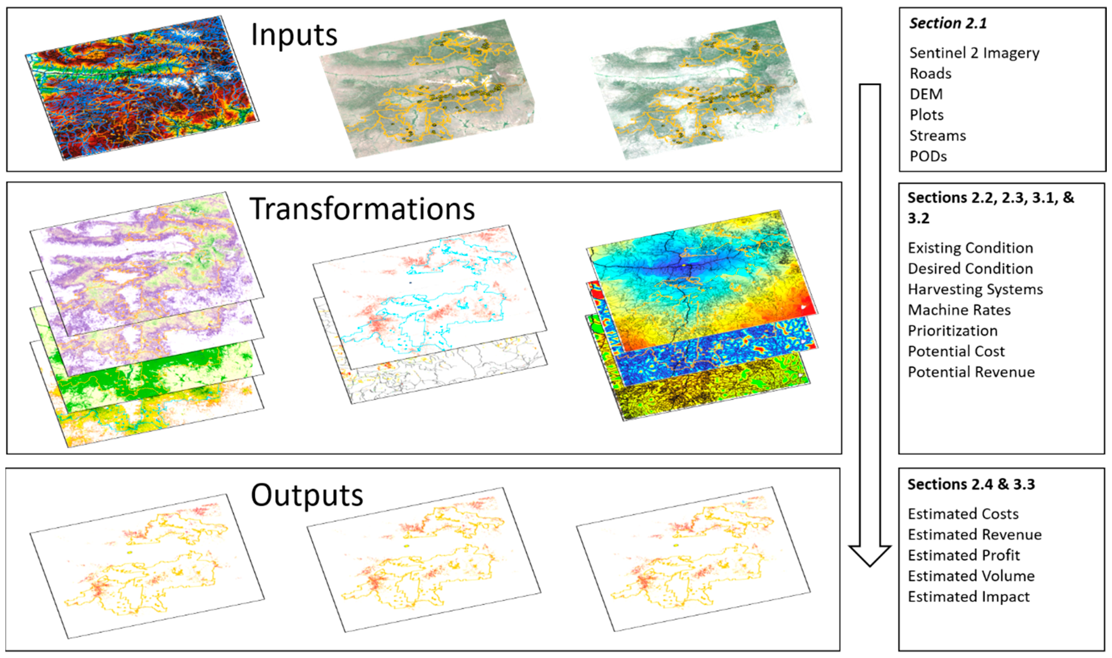
It is in this later context that we present a case study in the Blue Mountains of Oregon, USA. Our case study highlights new and novel computational tools and techniques used to create fine-grained timely information that accurately describes the existing condition of forest lands and integrates seamlessly with wildfire risk, spread, and suppression analyses to quantify prescription costs and anticipated revenues for forest plan implementation. Case study objectives include: (1) to quantify the existing forest condition using remotely sensed imagery, field data, the Rocky Mountain Research Station (RMRS) Raster Utility spatial modeling tools [22], and ensemble of generalized additive models (EGAMs) [23]; (2) to spatially define desired future condition and prescriptions that leverage the Potential Operational Delineations (PODs) framework to both harden fire control boundaries and bring POD interiors to a more fire-resilient condition; and (3) to spatially map a cost revenue assessment (CRA) that quantifies the existing supply chain and delivered costs [24] associated with implementing desired future conditions (Figure 1). Using these spatially explicit datasets, the RMRS Raster Utility spatial modeling tools, batch processing, and function modeling [25], we then further demonstrate how managers can quickly and easily prioritize treatments based on wildfire risk, budgetary constraints, and anticipated revenues.

While the objectives of reducing potential fuel loads and restoring the surrounding landscape to a more fire-resilient condition are fairly straightforward, the logistics, planning, prioritizing, and optimization of future treatments are complex and require substantial amounts of finely detailed information to efficiently and effectively allocate limited resources. In large part, the lack of finely detailed information pertaining to the existing condition of the vegetation, the economics associated with various prescriptions, and the optimal spatial allocation of treatments used to reduce wildfire risk increases the uncertainty associated with various prescriptions and outcomes and adds to the complexity associated with planning and implementing effective and efficient management.

This is not to imply that little is known with regards to the grass, shrub, forested vegetative communities [26], fuels [27], fire spread [12], fire risk [28,29,30], and the anthropogenic infrastructure within the area. Instead, it highlights that while inventory efforts such as Forest Inventory Analysis (FIA) [31], multiparty monitoring plots [32], Topologically Integrated Geographic Encoding and Referencing (TIGER) road inventories [33], and derived products such as those produced by the Landfire project and Wildfire Risk Simulation Software (FSim) exist, these resources alone do not provide the wall-to-wall information needed, at the appropriate scales, to address the finely grained spatially explicit questions or the justification for related prescriptions designed to restore the landscape to a fire-resilient condition.

However, coupled with finely grained remotely sensed information, such as Sentinel 2 imagery [34] and the National Elevation Dataset (NED) [35], data such as multiparty monitoring plots and TIGER road networks and statistical and machine-learning relationships can be leveraged to produce finely grained surfaces depicting the existing forest condition [23] and the costs to move biomass from the forest to a given sawmill [24]. In this study, we demonstrate how existing forest monitoring plots [32], TIGER line files [33], Sentinel 2 imagery [34], and PODs derived from fire managers and common fire modeling tools [11] were used to quantify various forest metrics and treatment costs which in turn were used to inform, justify, and improve restoration decisions. Due to the variety of data sources used, the methodological steps outlined, and the specialized language of the fire, forest, geospatial, and statistical and machine-learning modeling communities, many acronyms are presented in this study. To aid in reading, we provide a list of all acronyms used in this study in Appendix A.

2. Materials and Methods

2.1. Study Site & Primary Data

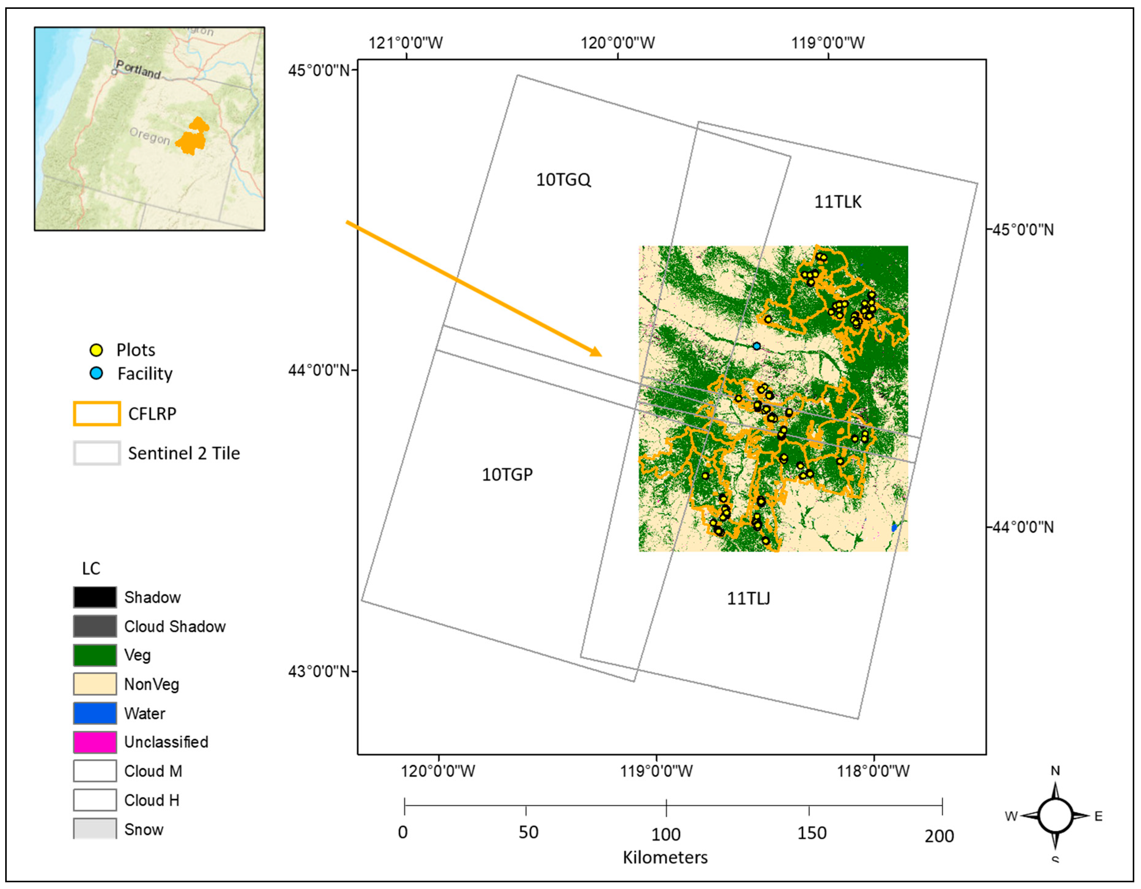
Our study site was located in eastern Oregon, USA and consists of both private and public lands, covering approximately 1.2 million ha (Figure 2). The study area encompasses 1 of 23 high-priority landscapes managed by the Forest Service that receives augmented funding from Congress to accelerate the pace and scale of restoration treatments under the Collaborative Forest Landscape Restoration Program (CFLRP) [36]. Vegetation types across this landscape include dry grasslands, shrubs, and pine and mixed conifer forest types [37]. This research utilized data from a long-term multiparty monitoring program, the Forest Vegetation and Fuels (FVF) program, led by Forest Service managers, Oregon State University researchers, and the Blue Mountains Forest Partners, a stakeholder group based in John Day, Oregon that convenes diverse stakeholders to help plan and implement restoration treatments on Forest Service lands [32]. The FVF program provides data that informs accelerated restoration in an adaptive management framework [38].

Historically, chronic surface fire across the study area removed fine surface fuels and promoted low-severity fire effects [39]. Fire exclusion policies have resulted in extremely high wildfire fuel loads [40] that, along with a warming climate, drive large fast-moving fires that threaten human communities and wildlife habitat [41,42,43]. Reducing forest density to facilitate reintroduction of low-severity fire is a major goal of accelerated restoration funded by the CFLRP [44].

Primary raster datasets used in the case study included NED 30 m digital elevation model [35] and Sentinel 2 satellite level 2a processed imagery [45] (

Table 1. A short list, description, and contribution of input datasets.

Name	Description	Contribution
Roads	TIGER\Line road network	Cost Revenue Assessment
Streams	NHD Flowline	Cost Revenue Assessment
Waterbodies	NHD Waterbodies	Cost Revenue Assessment
Plots	FVF field plots	Existing Condition
PODs	Potential Operational Delineations	Cost Revenue Assessment & Desired Future Condition
Facilities	Malheur Lumber Company	Cost Revenue Assessment
CFLRP	Collaborative Forest Landscape Restoration Program	Analysis extent
DEM	Digital Elevation Model	Existing Condition, Cost Revenue Assessment & Desired Future Condition
Sentinel 2	Satellite Imagery Bands (2–8, 8b, 11, and 12)	Existing Condition

TIGER = Topologically Integrated Geographic Encoding and Referencing, NHD = National Hydrograph Dataset, FVF = Forest Vegetation and Fuels Monitoring Program, POD = Potential Operational Delineations, CFLRP = Collaborative Forest Landscape, DEM = digital elevation model.

). Sentinel 2 satellite images were acquired for a spring and fall season during 2019 and consist of a total of eight tiles for spring and fall seasons (Figure 2, Table 1). Acquisition dates for spring and fall tiles fell on the same day within each season, had minimal cloud cover (<1%), and visually appeared to be at a common relative radiometric scale. As such, level 2a bottom of atmosphere products were used without further relative or absolute normalization. To address various grain sizes of the imagery and elevation datasets, all raster surface metrics used as predictor variables for modeling were resampled to a 30 m spatial resolution based on the environmental research institute’s (ESRI’s) nearest neighbor algorithm [46]. Primary vector datasets used included 2019 TIGER/Line files acquired from the US census bureau [33], Flowline and Waterbody line and polygon features from the National Hydrography Dataset (NHD) [47], FVF monitoring plots [32], POD polygons [11], and the location of the Malheur Lumber Company (Table 1).

2.2. Existing Condition

To quantify the existing condition of the landscape within a classical forest management perspective, at a fine spatial resolution, we employed an enhanced general additive modeling approach (EGAM) [23] that related summarized plot data to texture metrics derived from multitemporal Sentinel 2 level 2a processed satellite imagery [45] and topographic metrics derived from the NED digital elevation model (DEM) dataset [35]. The EGAM procedure extends generalized additive modeling (GAM) [48] by incorporating a Monte Carlo sampling scheme to create and independently test multiple GAM models as an ensemble. The ensemble of GAMs was then aggregated to produce estimates of response mean and standard error. As part of the EGAM procedure, predictor variables are iteratively selected from all potential predictor variables using all sample observations [49]. After selecting predictor variables, datasets are internally partitioned into training and test subsets to both build and independently test each model, respectively. For each response metric, a total of 50 GAMs were created using random subsets of 80% of the data to build the model and 20% of the data to independently test the model. To guard against extremely poor predictive models becoming part of the EGAM, we assigned a k-factor of 10 for regression-based models and an improvement factor of 0.02 for multinomial models. K and improvement factors were conservatively assigned to identify extremely poor performing models due to extreme samples. Once built, EGAMs were applied back to predictor surface to create continuous estimates of response variable mean and standard error. An implementation of the EGAM procedure can be found in [50].

Key response metrics derived from the monitoring plot data and used to describe the landscape included: cover type (Pine, Fir, or Nonforest), tree basal area measured in m² ha⁻¹ (BAH), the number of trees ha⁻¹ (TPH), bone dry tonnes (i.e., a metric ton or megagram) of stem wood biomass ha⁻¹ (SWBH), and bone dry tonnes of total above ground biomass ha⁻¹ (AGBH). BAH, TPH, SWBH, and AGBH were estimated for trees greater than 12.7 cm in diameter at breast height based on commonly used equations (

Table 2. List of forest response metrics and calculations used to summarize tree data by species (i) collected at each plot.

Metric	Equation	Source
DomType	Boolean logic selecting the species with the greatest BAH. Class labels include Nonforest (BAH = 0), Pine, and Fir.	NA
BAH	$\mathrm{EF}\ast \sum \frac{\pi {\mathrm{DBH}}^2}{40,000}$	[51]
TPH	EF * tree count	[51]
SWBH	${\displaystyle \sum }_i\mathrm{AGBH}\ast e^{\left(-0.3737+\frac{-1.8055}{\mathrm{DBH}}\right)}$	[52]
AGBH	$\mathrm{EF}\ast {\displaystyle \sum }_i{e}^{\left(b1+b2\ast \ln \left(\mathrm{DBH}\right)\ast 2.2046/2000\right)}\ast 2.2417$	[52]

BAH = basal area ha⁻¹ (m²), TPH = tree counts ha⁻¹, SWBH = stem wood biomass ha⁻¹, AGBH = above ground biomass ha⁻¹, EF = expansion factor for a given fixed plot radius, and b1 and b2 are species-specific coefficients in [52].

). Field plot data collection protocol is described in [32], and expansion factors (EF) for plot estimates were used to bring BAH, TPH, SWBH, and AGBH to the scale of a ha.

Likewise, predictor metrics were created at approximately the same spatial resolution as the extent of each monitoring plot and included mean and standard deviation derived from a 3 by 3 cell neighborhood window passed through each cell, within each image band of the Sentinel 2 imagery used in the analyses (

Table 3. List of raster metrics and calculation used to create predictor variable values collected at the location of each plot [25].

Metric	Description
Mean	Band cell mean value within a 3 by 3 moving window
Standard Deviation	Band cell standard deviation within a 3 by 3 moving window
Slope	Percent slope calculated from a digital elevation model
Northing	Northing calculation from azimuth
Easting	Easting calculation from azimuth

). Sentinel 2 image bands acquired at a spatial resolution of 20 m (i.e., 5–7, 8a, 11, and 12) were resampled to a spatial resolution of 10 m, using ESRI’s nearest neighbor algorithm, prior to performing neighborhood analyses. After performing neighborhood analysis, all raster surfaces were resampled to a 30 m spatial resolution to match the spatial resolution of topographic features and approximate the spatial resolution of the monitoring plots. Topographic features created for the EGAM included slope, northing, and easting and were created from the NED DEM and combined with Sentinel 2 images as potential predictor variables (Table 3).

FVF monitoring plots represent a collection of various systematically located field plots in randomly selected treatments units and nearby untreated controls designed to track changes in vegetation given different implemented treatments [32]. As such, when aggregated together they represent a sample biased to the treatments monitored across the landscape. To address this sampling bias and attempt to center our estimates to the population of pixels that make up our study site while also spreading our dataset across predictor variable space, we implemented a Generalized Random Tessellation Stratified (GRTS) [53] strategy to develop a comparison sample (CS). Our GRTS strategy uses the first two component scores of a correlation-based principal component analysis (PCA) [25,54,55,56] resulting from predictor variable values found at 100,000 randomly selected locations across the study area to create a sample of observations spread and balanced across predictor variable space [57,58,59]. Using the CS and the predictor variable values found at those locations, we then performed an unsupervised K-means clustering [25,54,60] of the observations, splitting the sample into 100 different K-mean classes. Next, we applied the same K-means algorithm [25,54] to our monitoring sample and compared the proportion of K-mean class counts found within the monitoring plot sample to the CS. K-mean classes that were over- or under-represented in the monitoring plots were then identified and labeled. Observations falling within K-mean classes labeled as over-represented in the monitoring plot sample were then randomly selected until class count proportions matched those of the CS. K-mean classes identified as being under-represented were then supplemented with additional monitoring plot locations randomly chosen across the study area, which met K-mean class criterion, until class count proportions matched. Newly assigned plots were spatially identified and scheduled to be collected during future field data collection campaigns.

2.3. Desired Future Condition (DFC) & Biomass Removal

The ideal or desired condition of the landscape can vary based on management objectives. For this study we narrowed the management objectives to bring Pine dominant forest cover types (DomType, Table 2) to BAH densities that generally resulted in reduced flame lengths (fire-resilient condition) and spread across POD containment zones. POD containment zones were previously delineated for the study area [11] and were prioritized into strategic response zones with the following labels: Protect, Restore, Maintain, Exclude, and High complexity (Appendix B). PODs serve as a natural mechanism to spatially compartmentalize the landscape and build prescriptions designed to generally reduce tree BAH within POD boundaries and further reduce tree densities at and around those boundaries. Using the results of [61] that describe the impacts to flame length based on basal area variable density thinning prescription across similar landscapes, we generated a series of rules that spatially identify desired future BAH, for each 30 m cell within the study area (

Table 4. Desired basal area ha⁻¹ (BAH) for the Pine and Fir * dominant forest cover types. Processing order identifies the priority of desired BAH threshold, in shared areas, given the selection rule.

Description	Rule	Order	Desired BAH
Slope	>50%	1	Existing
SMZ	Within 30 m	2	Existing
POD Boundary	Within 0.4 km	3	15 BAH
North Aspect	270–90° Azimuth	4	27 BAH
South Aspect	90–270° Azimuth	5	20 BAH

* Desired ΔBAH for Fir cover types were only different than 0 when cells were within 0.4 km of a POD boundary.

).

Primarily Pine dominant forest cover types (DomType, Table 2) were selected for potential treatment. However, next to POD boundaries, cells classified as Fir dominant cover types were also treated. Generally, variable density BAH thresholds for north facing slopes were 27 m² ha⁻¹, while south facing slope thresholds were 20 m² ha⁻¹. For areas within 0.4 km of a POD boundary, BAH thresholds were 15 m² ha⁻¹ and prescriptions were designed to harden POD boundaries and reduce the ability of fire to move across those boundaries. All perennial stream side management zones (SMZs, 30 m from a stream) were excluded from mechanical treatment (deferred). Likewise, areas with a slope greater than 50% were deferred due to operational constraints. To be relatively sure that modeled estimates of BAH were accurate, we excluded all cells that had BAH mean estimate that were not statistically different than zero at the 95% confidence level.

Using these rules, Batch Processing [25,62], elevation, slope, the results from the EGAM surfaces, and raster map algebra [63], we quantified how much biomass would need to be removed from each 30 m cell to meet the desired future condition (DFC, Figure 3). Removal values were calculated on a cell basis by subtracting the existing BAH from the DFC BAH (ΔBAH). The proportion of DFC BAH removed from the existing condition was then used to estimate the amount of SWBH (ΔSWBH) and AGBH (ΔAGBH) removed from the landscape as follows:

$$\Delta \mathrm{SWBH}=\frac{\Delta \mathrm{BAH}}{\mathrm{BAH}}\ast \mathrm{SWBH}\ast \left(1-\%\mathrm{leakage}\right)$$

(1)

$$\Delta \mathrm{AGBH}=\frac{\Delta \mathrm{BAH}}{\mathrm{BAH}}\ast \mathrm{AGBH}\ast \left(1-\%\mathrm{leakage}\right)$$

(2)

ΔSWBH and ΔAGBH were converted into sawlog (ST) and biomass (BT) tonne products removed from the landscape by incorporating leakage and cell area as follows:

$$\mathrm{ST}=\mathsf{\Delta }\mathrm{SWBH}\ast \left(1-\%\mathrm{leakage}\right)\ast 0.09$$

(3)

$$\mathrm{BT}=\left(\mathsf{\Delta }\mathrm{AGBH}-\mathsf{\Delta }\mathrm{SWBH}\right)\ast \left(1-\%\mathrm{leakage}\right)\ast 0.09$$

(4)

In Equations (3) and (4), % leakage represents the amount of woody biomass left on the landscape due to felling and processing and the constant 0.09 was used to convert ha⁻¹ estimates to cell area estimates. For ST, leakage was held constant at 5%. For BT, leakage was held constant at 50%. Cells with negative ΔSWBH and ΔAGBH that did not meet topographic or SMZ thresholds, or that had BAH estimates that were not statistically different than zero, were assigned ΔSWBH and ΔAGBH values of 0.

To address estimation variation in the decision-making process for existing condition continuous EGAMs (Section 3.1), raster surface cell standard error values were used to create a binary mask of estimates that were statistically different than zero. Using cell mean estimates, standard error estimates, and a z-score for two standard deviations from the mean (1.96), we created a binary mask identifying raster cells in which the 95% confidence interval of the mean included an estimate of zero. Cell values with estimated mean values including zero were remapped to a value of zero while cells with mean estimates statistically greater than zero (95% confidence interval) were given a value of one. Continuous response variable masks were then multiplied by EGAM estimates in Section 3.2 and Section 3.3 to zero out mean estimates and increase the confidence that the existing condition did not include a value of zero or below.

2.4. Cost Revenue Assessment (CRA)

Delivered cost was calculated using the model described in [24]. Cost in this context referred to all costs associated with felling, processing, and moving woody biomass from the forest to the Malheur Lumber Company conversion facility (Figure 2). The delivered cost model in [24] uses a least-cost path algorithm [64] to transform surface distances, both on- and off-road, into travel times based on specified harvesting systems and associated machine and operation rates (

Table 5. Cost components used to convert travel time into cost. Tonne mass units are presented as bone dry.

Component	Type	Value	Units
On-road	Machine Rate	90	USD h−1
	Speed	Table 6	km h−1
	Payload	25.40	tonne
Off-road	Machine Rate	80	USD h−1
	Speed	4.83	km h−1
	Payload	3.63	tonne
Operations	Harvesting & Processing	65	USD tonne−1
Other	Administrative	0	USD tonne−1

). For our study, rubber-tire-skidder-based systems were only considered for the implementation of mechanically based prescriptions. Of note, the delivered cost model can include barriers to motion for off-road travel. We used NHD perennial streams and waterbodies and TIGER\line U.S. interstate and state highways as barriers to motion for off-road travel.

Travel time was then converted to dollars tonne⁻¹ (bone dry) using cost hr⁻¹ operation rates (Table 5). Outputs from the delivered cost model included medium- to fine-grained raster surfaces that estimate total round-trip travel costs of off-road skidding and on-road transportation for each cell across the landscape. Inputs for this model included a TIGER\linear road network with rates of speed defined for each road segment (

Table 6. Queries used to allocate the average speed to each road segment and its derived raster cells, considering the Master Address File (MAF) TIGER\Line Feature Class Code (MTFCC) ¹.

Query	Speed km h−1
MTFCC = “S1400”: Local Road, Rural Road, City Street	88
MTFCC = “S1200”: Secondary road	56
MTFCC = “S1100”: Primary road	40
NOT (MTFCC = “S1400” OR MTFCC = “S1200” OR MTFCC = “S1100”)	40

¹ MTFCC codes and definitions can be found at: https://www.census.gov/geo/reference/mtfcc.html (accessed on 12 May 2021).

), the NED DEM, and cost components depicting the rates of speed

For moving biomass from the site of harvest to the roadside, hourly rates for machines use an average payload (tonnes trip⁻¹) for different types of equipment, fixed operations, administration cost (as a dollar tonne⁻¹ constant), and a vector layer of off-road barriers.

Operation costs of USD 65 tonne⁻¹ included felling (USD 15) and processing (USD 50), but not skidding, which is included in off-road travel cost accounting. The administrative costs were assumed to be zero to provide a normalized comparison across all forest ownerships. Together, on-road, off-road, and operation costs constituted the optimal potential total cost (OPTC) of moving biomass, measured in dollars tonne⁻¹, to Malheur Lumber Company in a spatially explicit manner, at the spatial resolution of 30 m² across the study site. The estimated actual cost of prescription implementation (ACPI) was then calculated by multiplying OPTC by the amount of biomass removed at each cell, where 0.09 converts ΔAGBH estimates to cell area estimates as follows:

$$\mathrm{ACPI}=\Delta \mathrm{AGBH}\ast 0.09\ast \mathrm{OPTC}$$

(5)

Like ACPI, estimated revenue is dependent on ΔAGBH. However, estimated revenue (ER) also depends on gate prices for various products removed from forests as follows:

$${\mathrm{ER}}_{\mathrm{saw}}={\mathrm{ST}\ast \mathrm{Gate}\mathrm{Price}}_{\mathrm{saw}}$$

(6)

$${\mathrm{ER}}_{\mathrm{biomass}}={\mathrm{BT}\ast \mathrm{Gate}\mathrm{Price}}_{\mathrm{biomass}}$$

(7)

We fixed gate prices for sawlogs at USD 55 green tonne⁻¹ and USD 28 green tonne⁻¹ for biomass products [65]. Assuming an average green moisture content of 94% [66], dry tonne gate price equivalents were estimated at USD 106.70 tonne⁻¹ for sawlogs and USD 54.32 tonne⁻¹ for biomass products. Using map algebra, function modeling, and Equations (6) and (7), we calculated saw and biomass ER for each 30 m cell and created spatially explicit raster surfaces. Adding saw and biomass ERs together, we calculated total ER. Finally, we subtracted ACPI from total ER for overlapping raster cells to create a raster surface of estimated anticipated income (EAI) of implementing a prescription as follows:

$$\mathrm{EAI}=\left({\mathrm{ER}}_{\mathrm{saw}}+{\mathrm{ER}}_{\mathrm{biomass}}\right)-\mathrm{ACPI}$$

(8)

3. Results

3.1. Quantifying Existing Condition

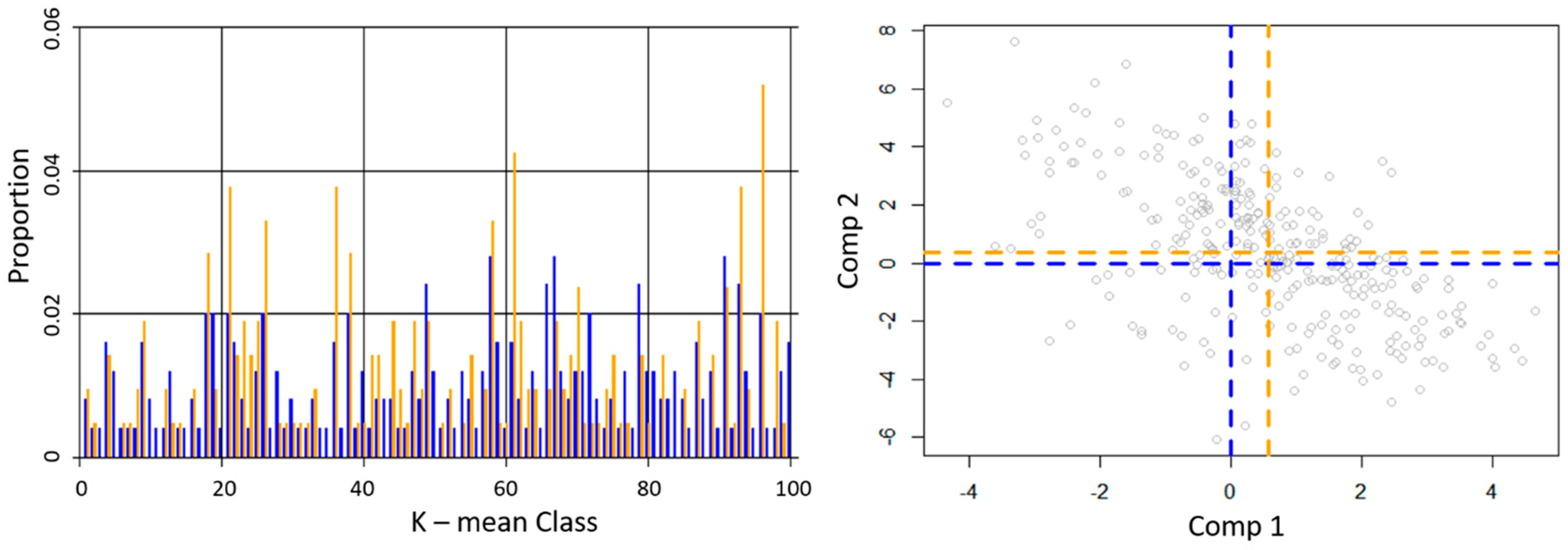
Our GRTS selection strategy selected 429 plots balanced and spread across the first two principal components of transformed predictor variable space. The first two principal components of our GRTS selection strategy accounted for 45% of the correlation within data. Of the 429 selected plots, 301 plots had been visited and were used to calibrate EGAMs. In total, 128 plots were identified for future field data collection campaigns. Ideally, EGAMs would be created after collecting the additional 128 plots. However, given the spread and approximate balance of this sample (Figure 4), we chose to use these plots to calibrate our EGAMs. From this sample, we expect global model bias, due to sampling, to be minimal and that interpolated model estimates across predictor variable space will approximate the relationship occurring within unsampled K-mean classes. Of importance with regards to estimation error in under-sampled regions of predictor variable space is the variability across GAMs within our EGAMs. To spatially identify those regions of predictor variable space we projected K-mean class into coordinate space and provided that binary map as a band within each of the raster surfaces.

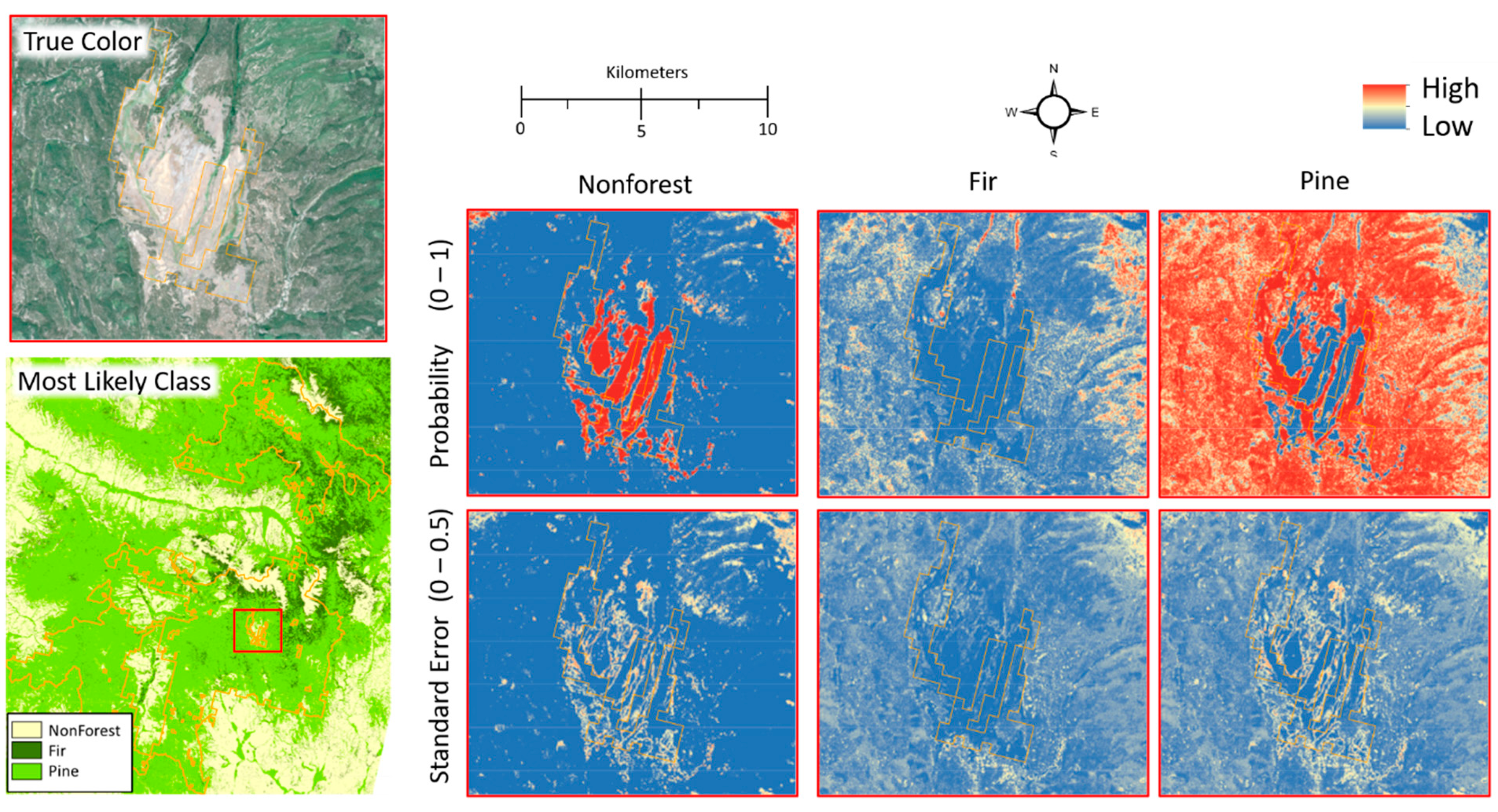
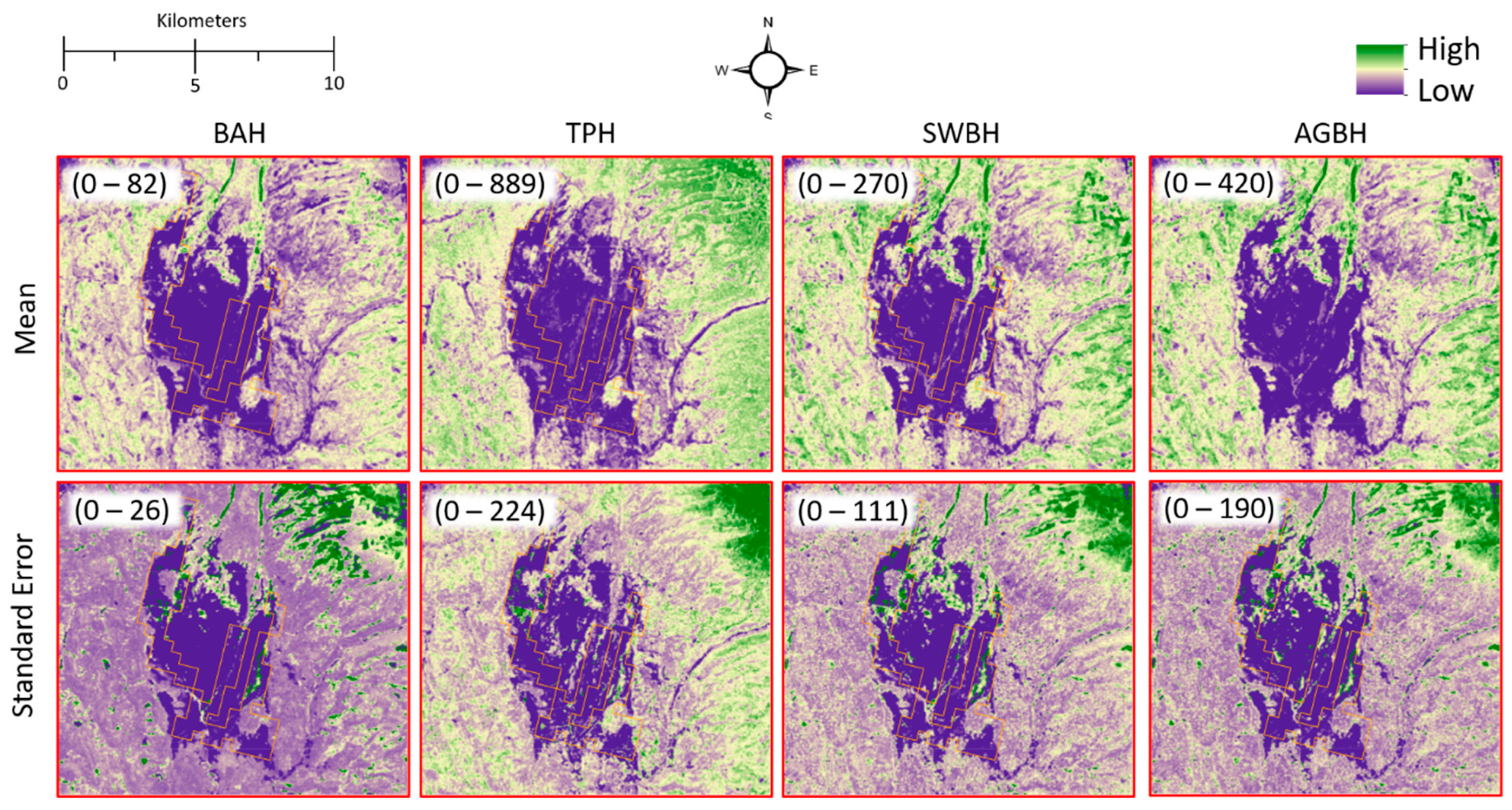
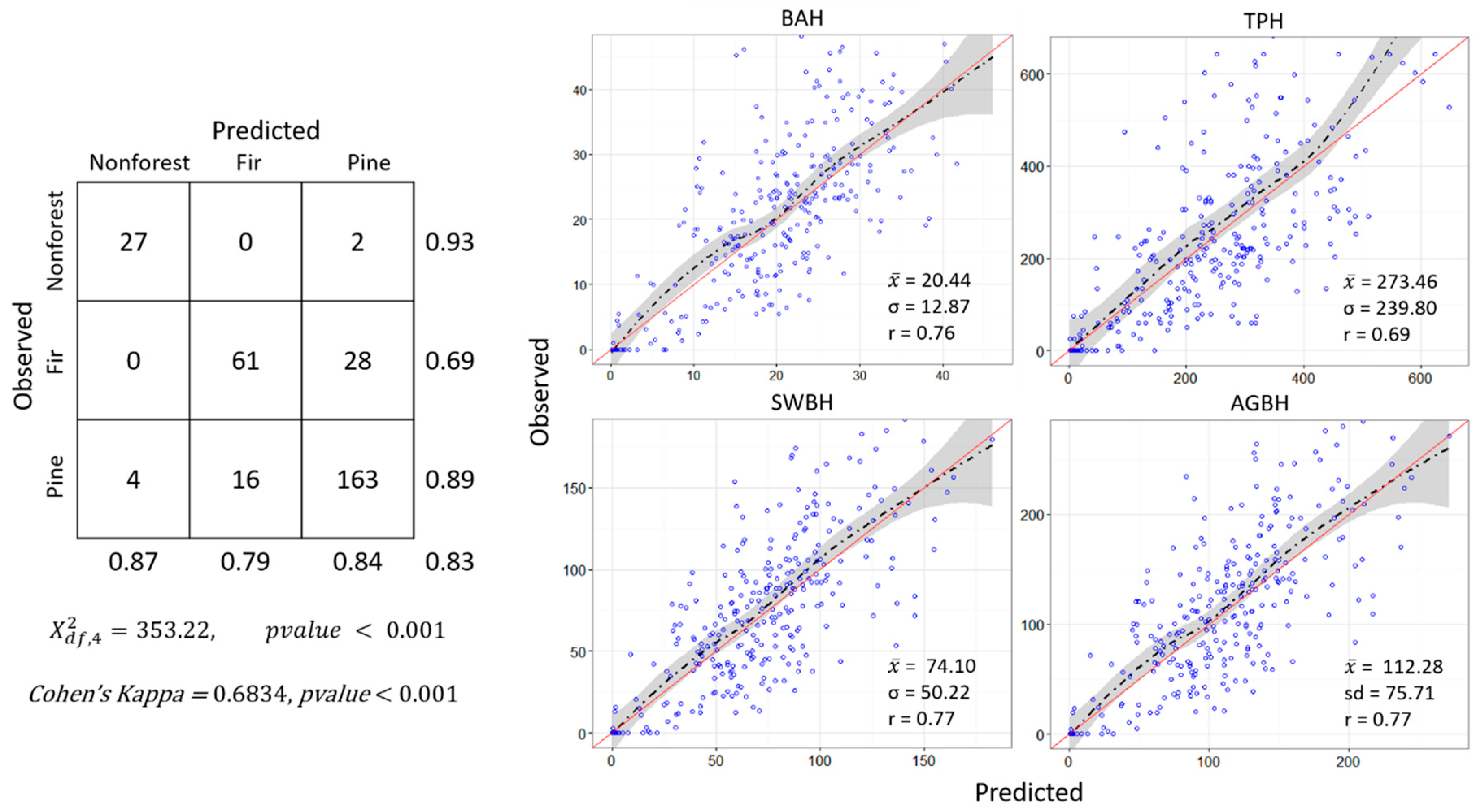
Using our sample of 301 observations, we created 50 GAMs from random subsets of the data and combined them together as an ensemble for each of our response variables. Statistically selected predictor variables identified in the selection process are presented in

Table 7. Ensemble of generalized additive models (EGAM) predictor variables and fit statistics using all observations. Root mean squared error and overall map accuracy are reported for continuous (a) and categorical (b) response variables.

EGAM	Source	Predictors	Fit
BAH (a)	Sentinel Mean	summer bands—7, 11, and 12 fall bands—6, 8b, and 12	8.36
	DEM	elevation and slope
TPH (a)	Sentinel Mean	summer band—12 fall bands—2, 11, and 12	176.06
	Sentinel Standard Deviation	summer band—5
	DEM	elevation and easting
SWBH (a)	Sentinel Mean	summer band—7, 11, and 12 fall bands—6, 8b, 12	32.44
	Sentinel Standard Deviation	fall band—6
	DEM	elevation and slope
AGBH (a)	Sentinel Mean	summer band—7, 11, and 12 fall bands—6, 8b, 12	48.81
	Sentinel Standard Deviation	fall band—6
	DEM	elevation and slope
DomType (b)	Sentinel Mean	summer band—4, 6, 7, 8, 11, and 12 fall bands—2	83.38%
	Sentinel Standard Deviation	fall band—2
	DEM	elevation

. On average the selection process reduced the potential number of predictor variables from 44 to 8.4 for each EGAM. The mean and standard deviation of estimates from all GAMs within each EGAM were used to populate raster surface band cell mean and standard error values (Figure 5 and Figure 6). EGAM fit statistics are presented in Table 7 and Figure 7 and on average explain 55.99% of the variation in the data for continuous responses and had an average map accuracy of 83.38% for the dominant forest classification. Of particular interest in Figure 7 is the overall strength of the relationship between observed and predicted values and the nonconstant variation in estimated values.

3.2. Desired Future Condition & Biomass Removals

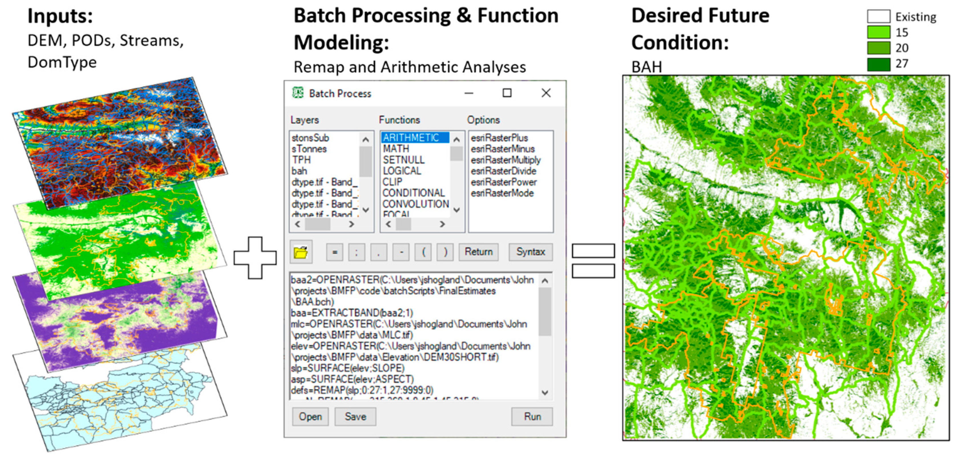
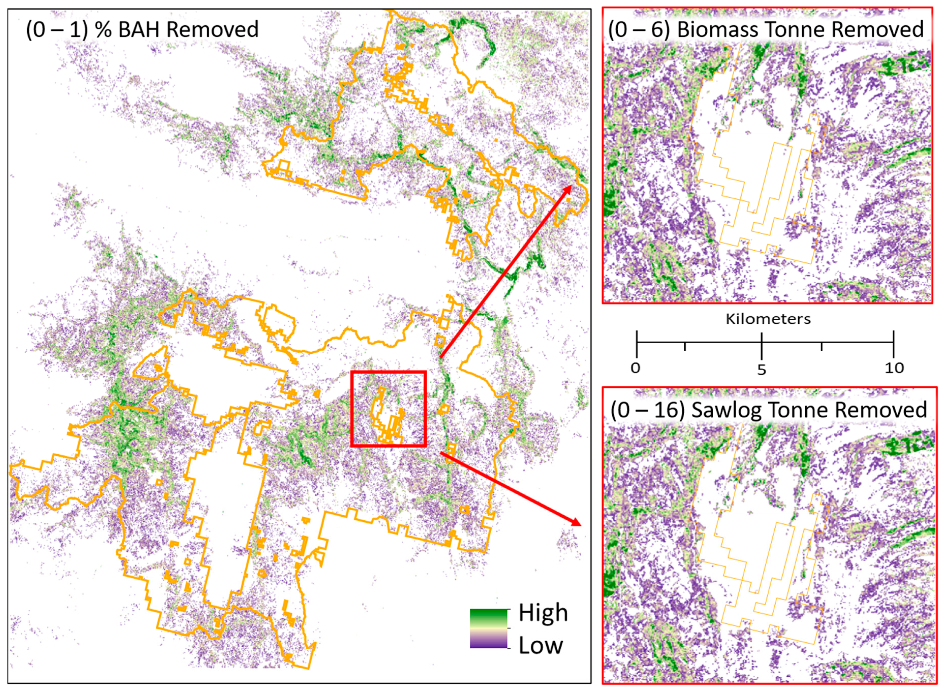
Using the Pine dominant forest type class, the DEM, stream networks, POD boundaries, batch processing, function modeling, and the rules described in Table 4, we were able to create a raster surface that spatially defined the DFC of a landscape in terms of BAH (Figure 3). Subtracting DFC from the existing BAH raster surfaces, we spatially quantified the reduction in BAH needed to meet DFC. Applying the proportion change in BAH to existing SWBH and AGBH surfaces and incorporating leakage (Equations (3) and (4)), we created two raster surfaces depicting the ST and BT removed from the landscape to meet DFC (Figure 8).

Approximately 527,000 ha across the study area had negative ΔBAH. Those cells represented areas in which the existing BAH was less than the DFC and as such were remapped to zero tonnes removed. Conversely, there were approximately 236,000 ha identified across the study area as having more BAH than desired. In many locations (approximately 86,000 ha) ΔBAH was relatively small (<4 m² ha⁻¹), suggesting minimal deviation from the desired future condition that may be of less importance to treat than cells with larger ΔBAH.

To meet DFC, approximately 6.5 and 0.9 million tonnes of sawlog and biomass products, respectively, will need to be removed from the landscape. Interestingly, while POD hardening zones account for only 22.66% of the total study area, the majority of tonnes removed to meet DFC came from those zones (approximately 54%). Fortunately, many of the POD boundaries were drawn along road networks, potentially reducing implementation costs associated with meeting wildfire objectives.

3.3. Cost Revenue Assessment

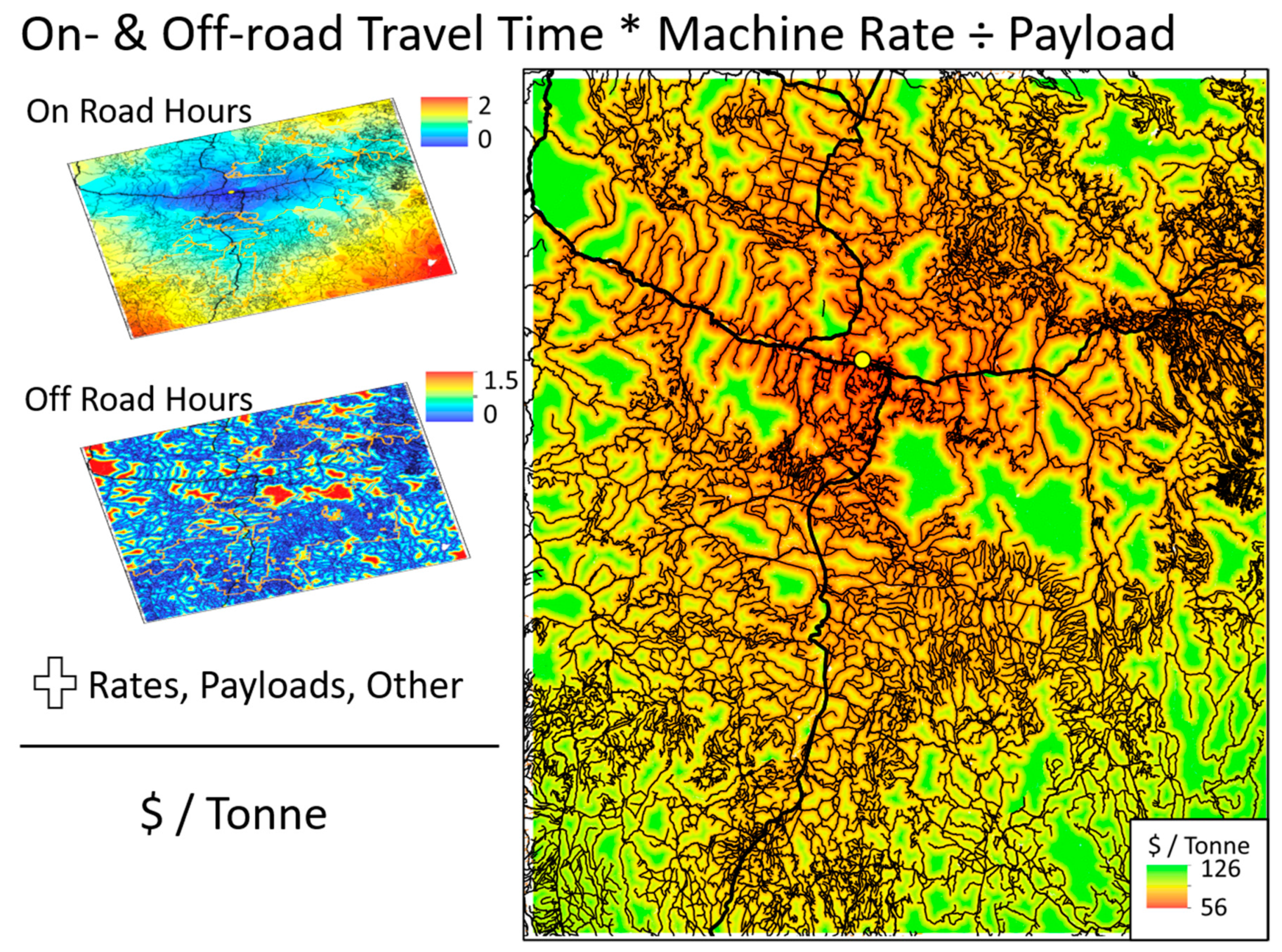
We spatially quantified OPTC and travel time for on- and off-road costs (Figure 9). Using batch processing, function modeling, machine rates, and payloads (Table 5), and the outputs from the delivered cost tool, we transformed travel times into dollars tonne⁻¹ raster surfaces that can be easily manipulated within batch processing and function modeling.

Approximately, 77% of the study area had a delivered OPTC between USD 60 and USD 70 tonne⁻¹. Only 6% of the landscape had a delivered OPTC less than USD 60 tonne⁻¹ and 17% of the study area had a delivered OPTC more than USD 70 tonne⁻¹. Moreover, there were no locations across our study area that had an estimated delivered OPTC less than USD 54.32, suggesting biomass products alone will produce negative profits.

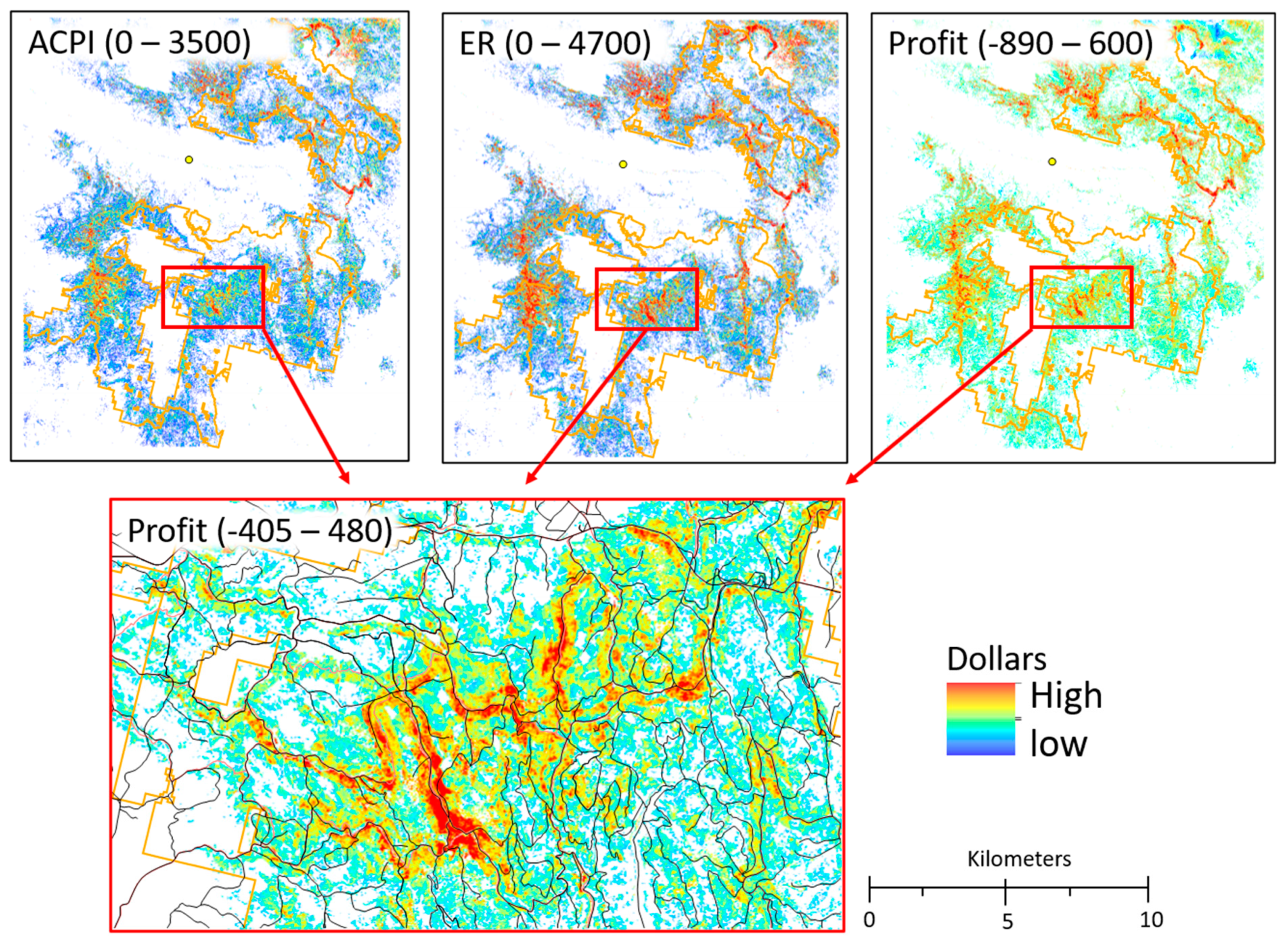
While the delivered OPTC identified costs on a tonne basis, the ACPI was dependent on the amount of total biomass tonne removed. On a cell basis we used map algebra and Equation (6) to spatially quantify ACPI (Figure 10). To meet DFC across the landscape would cost approximately USD 648 million. However, only 52% of that total cost was attributed to hardening POD boundaries. Moreover, 94% of the total ACPI area occurred within cells having an OPTC less than USD 70 tonne⁻¹, suggesting that restoring the landscape to DFCs would result in positive profits if a component of the prescription produced sawlog products (i.e., sawlog gate prices will offset delivered costs).

Like ACPI, ER for sawlog and biomass products was dependent on the amount of total biomass tonne removed from the landscape. Unlike ACPI, though, leakage and product type were factored into the estimated amount of ST and BT delivered to Malheur Lumber Company (Equations (3) and (4)). On a cell basis, we accurately estimated ${\mathrm{ER}}_{\mathrm{saw}}$ and ${\mathrm{ER}}_{\mathrm{biomass}}$ using Equations (6) and (7) (Figure 10). Profit margins were then calculated and spatially depicted by subtracting ACPI from total ER $\left({\mathrm{ER}}_{\mathrm{saw}}+{\mathrm{ER}}_{\mathrm{biomass}}\right)$ on a cell basis (Figure 10).

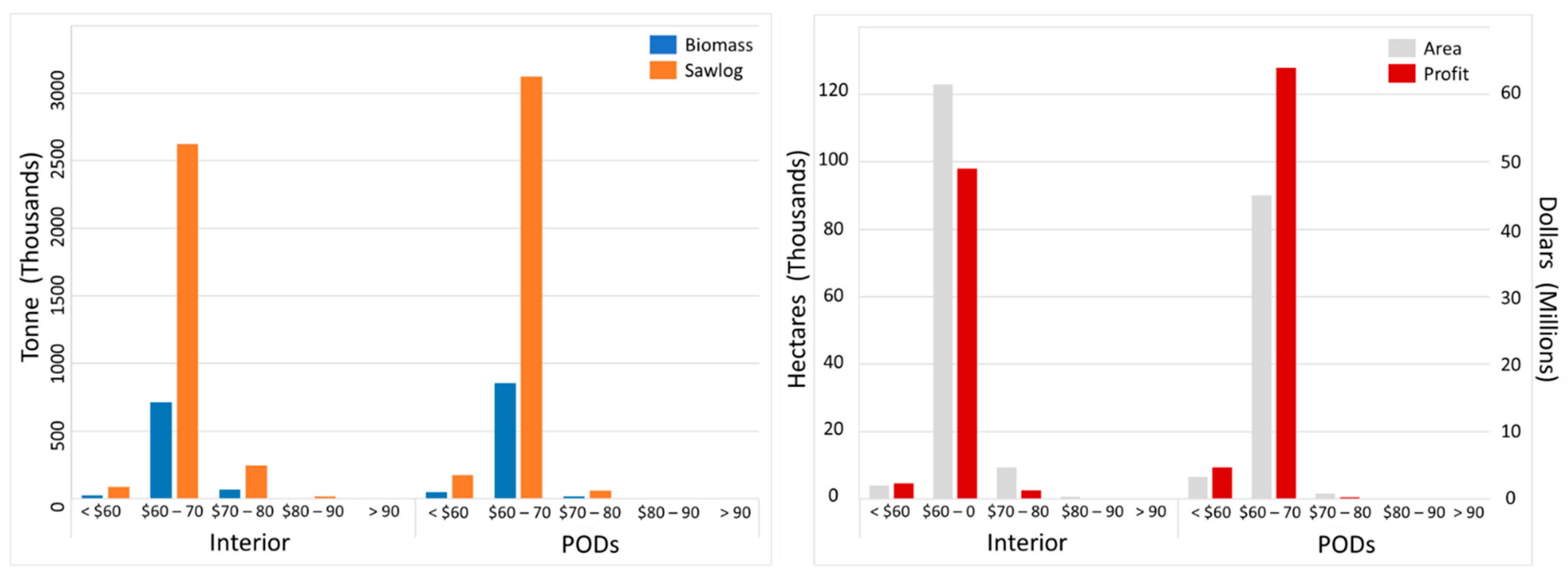
Approximately 99% of the area identified as needing treatment had a positive profit margin, suggesting that most of the landscape that departed from DFC had enough sawlog products to compensate for delivered costs. If all prescriptions were implemented across the landscape, we estimated a net positive profit of USD 121 million with an average positive return of USD 513 ha⁻¹. However, more than 80% of all Profit cell values had dollar ha⁻¹ estimates less than USD 513, suggesting marginal returns for most operational units. Relatively speaking, hardening POD boundaries returned larger net profits than prescriptions designed to increase fire resilience (Figure 11).

4. Discussion

Optimal decision making requires detailed and accurate information. We present a methodology that uses function modeling [25], batch processing [62], field plot data, and readily available information to create spatially explicit metrics used within the field of forestry to manage forests and fuels. Our approach builds on the outputs of common fire risk and simulation models by converting field plots and passively acquired remotely sensed data into raster surfaces that contain values of commonly used and well-known forest management metrics, spatially tied to fire risk and spread through PODs. Additionally, using a spatially explicit modeling approach we quantified the cost of delivering wood products to a specified processing location [24]. Moreover, using batch processing and map algebra, we transformed prescriptions designed to increase fire resilience and harden POD permitters into spatially explicit representations of DFC and further used those DFCs to quantify tree biomass removal. Finally, we combined each of those products at the cell level (spatial resolution of 30 m) to spatially identify and quantify various aspects of implementing treatments to meet DFCs.

Our analyses provide unique insights into both scale and application. Of note, the process of linking field plot data with Sentinel 2 multitemporal imagery using EGAMs allowed us to quickly and easily create 30 m raster surfaces depicting various mean metrics and estimates of standard error that can be used to manage forests at various spatial scales. These mean metrics and estimates of mean error provide practitioners with accurate, spatially explicit information pertaining to the forested condition at a spatial resolution that can be easily evaluated based on known forest practices and can be used to inform decision making. In our study, we demonstrated how these estimates (Section 3.1) coupled with DFCs (Section 3.2) can be used to quantify the amount of biomass removed from the landscape to both harden POD boundaries and restore forests to a more fire-resilient condition. Moreover, we demonstrated how estimates of mean error can be used to focus our restoration efforts on locations that have mean BAH estimates different than zero (95% confidence limits).

While our EGAMs accounted for much of the variation in the data (Section 3.1), improvements in model estimation error can be made by collecting additional field plots within under-represented portions of predictor variable space and portions of predictor variable space with large standard error estimates. Moreover, mean and standard error estimates can further be used with additional sampling and design-based estimators (e.g., ratio estimation [67]) to improve mean and total basal area, tree count, and biomass estimates for subregions (stands) within the study area. However, given the spread and balance of our sample and the fit of our existing condition models, we feel confident that our estimates can be used to help inform and prioritize prescriptions across the study area to reduce wildfire risk and increase resilience to wildfire.

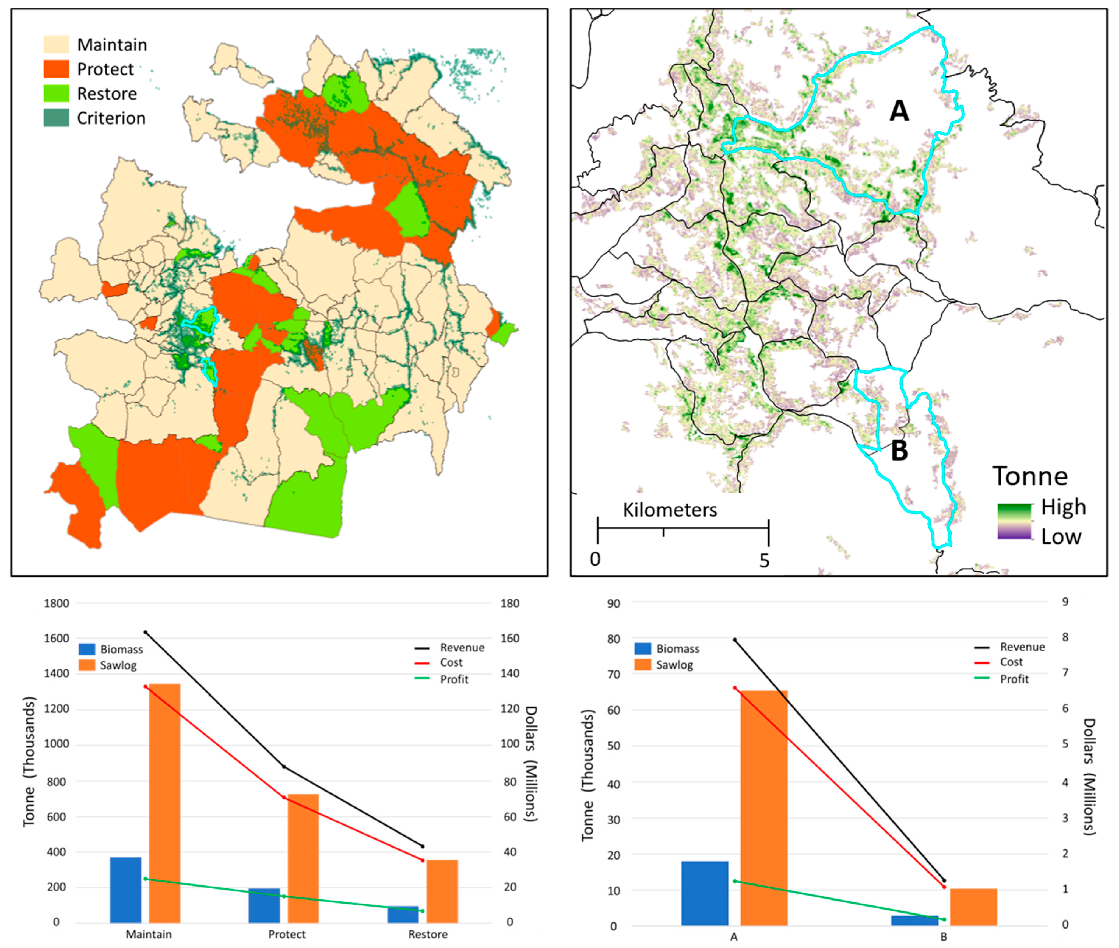
Coupled with known information related to variable density treatments [61], fire severity [68], wildfire risk [29,30], and the conceptual idea behind PODs [11], these types of spatially explicit raster surfaces provide information that can be easily manipulated within a geographic information system (GIS) to prioritize multiple objectives and compare and contrast alternatives [69]. For example, with these types of datasets we can prioritize and summarize biomass removal and retention, cost and revenue of implementation, and profit using POD boundaries. We can further use these datasets to develop and summarize quality risk assessment metrics and a series of spatial filters that take into consideration contiguous areas with enough biomass to justify operations (Figure 12). Moreover, we can compare coarse wildfire restoration strategies such as Maintain, Protect, and Restore, across strategies and among PODs at fine spatial scales. Additionally, using spatial adjacency rules and estimates of standard errors, we can filter and define operational treatment units that are at least 5 ha in size and that have at least three tonne of biomass on a cell basis (95% confidence interval threshold). Finally, treatment unit geometry can be used to summarize removals, costs, revenues, and profits at the treatment unit level.

Although Section 3.2 provides estimates of woody biomass removed to meet DFC, implementation costs often constrain where and the types of treatments that can occur. Our CRA estimates spatially quantify those costs and revenues for a snapshot in time given described machine rates and gate prices. As such, these estimates are dependent on the systems specified and can vary by operation. However, using batch processing, function modeling, and the delivered cost model, machine rates and gate prices can be adjusted quickly and easily. Additionally, these rates can be spatially allocated as raster surfaces within the delivered cost model to specify unique cost structures given various conditions [69]. Moreover, because CRA surfaces are spatially defined, additional costs not defined in our analyses can easily be incorporated into the CRA analysis on a ha⁻¹, tonne⁻¹, and spatially explicit basis. For example, both the cost of prescribed burning and road maintenance were not defined within our CRA. These costs can easily be added to the overall cost associated with implementation in a spatially explicit manner using batch processing and map algebra. Likewise, gate prices can vary from one sawmill to another and can be modified easily within the batch processing modeling framework. Because estimates of removed biomass are spatially identified, gate prices can also be allocated in a spatially explicit manner, providing flexibility in quantifying various prescriptions.

While changes to machine rates and gate prices and additional costs will change the overall cost, revenue, and profit surfaces, the spatial nature of these estimates provides flexibility in determining actual treatment costs and revenues. Moreover, these surfaces can be used to identify areas with limited access and financially justify treatments.

Generally, we recommend using the CRA surfaces to quantify the costs and revenue of prescriptions designed to meet forest objectives. However, cost and revenue surfaces could also be used for treatment optimization. Regardless of how they are used, it is important to recognize that machine rates and gate prices vary based on markets, and as such, the variability of markets, machine rates, and assumed prices should be factored into the planning and decision-making process.

In our CRA, the cost of felling and processing non-sawlog biomass was greater than gate prices. This suggests that to have positive net profits, sawlog biomass must be a component of the treatment. All prescriptions in our study included sawlog biomass products, so net positive profits were realized for approximately 99% of the landscape identified with more BAH than DFC thresholds. However, this does not mean that all cells with a net positive profit are practical to treat. Further thresholding, such as is depicted in Figure 12, may need to be employed to help identify operational treatment units that are practical.

Likewise, delivered cost for our CRA represents an optimal cost. That is, landings to which biomass are skidded are identified based on the least cost path to each individual 30 m road cell. Thus, the true cost associated with skidding material to a given landing will be more for all cells that are not defined as the least cost path. If landing locations are known prior to performing the delivered cost model, they can be incorporated into the analyses.

Finally, our data-driven approach to identifying, describing, and quantifying existing conditions, desired future conditions, and costs and revenues in a finely grained, spatially explicit manner across broad landscapes necessitates the use of spatial modeling, remote sensing, machine learning, and statistics. In many instances, this dependency will require translating GIS analyses into actionable information that practitioners can use to inform decision making [70]. While we recognize this to be a substantial hurdle to adoption, we argue that a larger emphasis must be placed on building those skillsets and integrating them within natural resource management.

5. Conclusions

We present an accurate, finely grained, spatially explicit approach to quantifying forest characteristics, desired future conditions, and the expected cost and revenues of implementing prescriptions designed to reduce wildfire risk and increase forest resistance to wildfire. Our approach leverages field plots, spatial, statistical, and machine-learning tools, and readily available datasets such as remotely sensed imagery, existing road and water networks, and elevation models to accurately quantify various aspects of restoring the forest landscape to a more fire-resilient condition. These spatially explicit datasets provide the types of information needed to meaningfully inform data-driven decision making.

References

- Kenward, A.; Sanford, T.; Bronzan, J. Western Wildfires: A Fiery Future; Climate Central: Princeton, NJ, USA, 2016; p. 42. [Google Scholar]
- USDA Forest Service. Towards Shared Stewardship across Landscapes: An Outcome-Based Investment Strategy; FS-118; USDA Forest Service: Washington, DC, USA, 2018.
- USDA Forest Service. The Rising Cost of Fire Operations: E_ects on the Forest Service’s Non-Fire Work. Available online: http://www.bren.ucsb.edu/academics/documents/Rising_Cost_Wildfire_Ops.pdf (accessed on 25 April 2020).
- Palaiologou, P.; Essen, M.; Hogland, J.; Kalabokidis, K. Locating Forest Management Units Using Remote Sensing and Geostatistical Tools in North-Central Washington, USA. Sensors 2020, 20, 2454. [Google Scholar] [CrossRef] [PubMed]
- Merschel, A.G.; Beedlow, P.A.; Sahw, D.C.; Woodruff, D.R.; Lee, H.E.; Cline, S.P.; Comeleo, R.L.; Hagmann, R.K.; Reilly, M.J. An ecological perspective on living with fire in ponderosa pine forest of Oregon and Washington: Resistance, gone but not forgotten. Trees For. People 2021, 4, 100074. [Google Scholar] [CrossRef]
- Miller, J.D.; Safford, H.D.; Crimmins, M.; Thode, A.E. Quantitative Evidence for Increasing Forest Fire Severity in the Sierra Nevada and Southern Cascade Mountains, California and Nevada, USA. Ecosystems 2009, 12, 16–32. [Google Scholar] [CrossRef]
- Cansler, C.; McKenzie, D. Climate, fire size, and biophyusical setting control fire severity and spatial pattern in the northern Cascade Range, USA. Ecol. Soc. Am. 2014, 24, 1037–1056. [Google Scholar]
- Balch, J.; Bradley, B.; Abotzoglou, R.; Nagy, R.C.; Fusco, E.; Mahood, A.L. Human-started wildfires expand the fire niche across the United States. Proc. Natl. Acad. Sci. USA 2017, 114, 2946–2951. [Google Scholar] [CrossRef] [Green Version]
- Foley, M. The High Cost of Wildfire in 2018. In NFPA; 2019; Available online: https://www.nfpa.org/News-and-Research/Publications-and-media/NFPA-Journal/2019/November-December-2019/Features/Large-Loss/Wildfire-Sidebar (accessed on 12 May 2021).
- Rice, B. Statement to Oversight Hearing on Wildland Fire Management: Federal and Non-Federal Collaboration, Including Through the Use of Technology, to Reduce Wildland Rire Risk to Communities and Enhance Firefighting Safety and Effectiveness. 2017. Available online: https://www.doi.gov/ocl/wildfire-management (accessed on 12 May 2021).
- Dunn, C.J.; O’Connor, C.D.; Abrams, J.; Thompson, M.P.; Calkin, D.E.; Johnston, J.D.; Stratton, R.; Gilbertson-Day, J. Wildfire risk science facilitates adaptation of fire-prone social-ecological systems to the new fire reality. Environ. Res. Lett. 2020, 15, 1–13. [Google Scholar] [CrossRef]
- Finney, M.A. An Overview of FlamMap Fire Modeling Capabilities. In Fuels Management—How to Measure Success: Conference Proceedings, Portland, OR, USA, 28–30 March 2006; Proceedings RMRS-P-41; United States Department of Agriculture: Washington, DC, USA, 2006; pp. 213–220. [Google Scholar]
- Carbone, A.; Jensen, M.; Sato, A. Challenges in data science: A complex systems perspective. Chaos Solitons Fractals 2016, 90, 1–7. [Google Scholar] [CrossRef]
- Elshawi, R.; Sakr, S.; Talia, D.; Trunflo, P. Big Data Systems Meet Machine Learning Challenges: Towards Big Data Sciences as a Service. Big Data Res. 2018, 14, 1–11. [Google Scholar] [CrossRef] [Green Version]
- Fernandes, P.; Botelho, H. A review of prescribed burning effectiveness in fire hazard reduction. Int. J. Wildland Fire 2003, 12, 117–128. [Google Scholar] [CrossRef] [Green Version]
- Kolden, C. We’re Not Doing Enough Prescribed Fire in the Western United States to Mitigate Wildfire Risk. Fire 2019, 2, 30. [Google Scholar] [CrossRef] [Green Version]
- Hiers, J.K.; O’Brien, J.J.; Varner, M.; Butler, B.W.; Dickinson, M.; Furman, J.; Gallagher, M.; Godwin, D.; Goodrick, S.L.; Hood, S.M.; et al. Prescribed fire science: The case for a refined research agenda. Fire Ecol. 2020, 16, 1–15. [Google Scholar] [CrossRef] [Green Version]
- Thompson, M.P.; Wei, Y.; Calkin, D.E.; O’connor, C.D.; Dunn, C.J.; Anderson, N.M.; Hogland, J.S. Risk Management and Analytics in Wildfire Response. Curr. For. Rep. 2019, 5, 226–239. [Google Scholar] [CrossRef] [Green Version]
- Baig, M.J.; Shuib, L.; Yadegaridehkordi, E. Big data adoption: State of the art and research challenges. Inf. Process. Manag. 2019, 56, 102095. [Google Scholar] [CrossRef]
- Côrte-Real, N.; Ruivo, P.; Oliveira, T. Leveraging internet of things and big data analytics initiatives in European and American Firs: Is data quality a way to extract business value? Inf. Manag. 2020, 57, 103141. [Google Scholar] [CrossRef]
- Thompson, M.P.; MacGregor, D.G.; Dunn, C.J.; Calkin, D.E.; Phipps, J. Rethinking the Wildland Fire Management System. J. For. 2018, 116, 382–390. [Google Scholar] [CrossRef] [Green Version]
- RMRS. RMRS Raster Utility. 2014. Available online: http://www.fs.fed.us/rm/raster-utility (accessed on 7 June 2021).
- Hogland, J.; Affleck, D.L.R.; Anderson, N.; Seielstad, C.; Dobrowski, S.; Graham, J.; Smith, R. Estimating Forest Characteristics for Longleaf Pine Restoration Using Normalized Remotely Sensed Imagery in Florida USA. Forests 2020, 11, 426. [Google Scholar] [CrossRef]
- Hogland, J.; Anderson, N.; Chung, W. New geospatial approaches for efficiently mapping forest biomass logistics at high resolution over large areas. Int. J. Geo-Inf. 2018, 7, 156. [Google Scholar] [CrossRef] [Green Version]
- Hogland, J.; Anderson, N. Function modeling improves the efficiency of spatial modeling using big data from remote sensing. Big Data Cogn. Comput. 2017, 1, 3. [Google Scholar] [CrossRef] [Green Version]
- LANDFIRE. LANDFIRE: Vegetation. U.S. Department of Agriculture and U.S. Department of the Interior. Available online: https://landfire.gov/vegetation.php (accessed on 7 August 2021).
- LANDFIRE. LANDFIRE: Fuel. U.S. Department of Agriculture and U.S. Department of the Interior. Available online: https://landfire.gov/fuel.php (accessed on 7 August 2021).
- Thompson, M.P.; Vaillant, N.M.; Haas, J.R.; Gebert, K.M.; Stockmann, K.D. Quantifying the potential impacts of fuel treatments on wildfire suppression costs. J. For. 2012, 111, 49–58. [Google Scholar] [CrossRef] [Green Version]
- Finney, M.A.; Mchugh, C.W.; Stratton, R.D.; Riley, K.L. A simulation of probabilistic wildfire risk components for the continental United States. Stoch. Environ. Res. Risk Assess. 2011, 25, 973–1000. [Google Scholar] [CrossRef] [Green Version]
- Thompson, M.P.; Calkin, M.A.; Finney, M.A.; Ager, A.A.; Gilbertson-Day, J.W. Integrated national-scale assessment of wildfire risk to human and ecological values. Stoch. Environ. Res. Risk Assess. 2011, 25, 761–780. [Google Scholar] [CrossRef]
- U.S. Department of Agriculture Forest Service (USFS). Forest Inventory and Analysis National Core Field Guide: Field Data Collection Procedures for Phase 2 Plots, 2019 Version 9.0. Vol. 1. Internal Report. Available online: https://www.fia.fs.fed.us/library/field-guides-methods-proc/docs/2019/core_ver9-0_10_2019_final_rev_2_10_2020.pdf (accessed on 14 May 2021).
- Johnston, J.D.; Greenler, S.M.; Miller, B.A.; Reilly, M.J.; Lindsay, A.A.; Dunn, C.J. Diameter limits impede restoration of historical conditions in dry mixed-conifer forests of eastern Oregon, USA. Ecosphere 2021, 12, e03394. [Google Scholar] [CrossRef]
- USCB. TIGER/Line Shapefiles [Machine-Readable Data Files]. Available online: https://www2.census.gov/geo/tiger/TGRGDB20/ (accessed on 12 May 2021).
- Earth Observing System [EOS]. Sentinel-2. Available online: https://eos.com/sentinel-2 (accessed on 5 December 2019).
- Gesch, D.; Oimoen, M.; Geenlee, S.; Nelson, C.; Steuck, M.; Tyler, D. The National Elevation Dataset. Photogramm. Eng. Remote Sens. 2002, 68, 5–11. [Google Scholar]
- Schultz, C.A.; Jedd, T.; Beam, R.D. The collaborative forest landscape restoration program: A history and overview of the first projects. J. For. 2012, 110, 381–391. [Google Scholar] [CrossRef]
- Simpson, M. Forested Plant Associations of the Oregon East Cascades; Technical Paper R6-NR-ECOL-TP-03-2007; USDA Forest Service, Pacific Northwest Region: Portland, OR, USA, 2007.
- Johnston, J.D.; Greenler, S.M.; Reilly, M.J.; Webb, M.R.; Merschel, A.G.; Johnson, K.N.; Franklin, J.F. Conservation of Dry Forest Old Growth in Eastern Oregon. J. For. 2021, 1, 13. [Google Scholar]
- Johnston, J.D.; Bailey, J.D.; Dunn, C.J.; Lindsay, A.A. Historical fire-climate relationships in contrasting interior Pacific Northwest forest types. Fire Ecol. 2017, 13, 18–36. [Google Scholar] [CrossRef]
- Hessburg, P.F.; Agee, J.K. An environmental narrative of inland northwest United States forests, 1800–2000. For. Ecol. Manag. 2003, 178, 23–59. [Google Scholar] [CrossRef]
- Jones, G.M.; Gutiérrez, R.J.; Kramer, H.A.; Tempel, D.J.; Berigan, W.J.; Whitmore, S.A.; Peery, M.Z. Megafire effects on spotted owls: Elucidation of a growing threat and a response to Hanson et al. (2018). Nat. Conserv. 2019, 37, 31. [Google Scholar] [CrossRef]
- Sankey, J.B.; Kreitler, J.; Hawbaker, T.J.; McVay, J.L.; Miller, M.E.; Mueller, E.R.; Vaillant, N.M.; Lowe, S.E.; Sankey, T.T. Climate, wildfire, and erosion ensemble foretells more sediment in western USA watersheds. Geophys. Res. Lett. 2017, 44, 8884–8892. [Google Scholar] [CrossRef] [Green Version]
- Williams, J. Exploring the onset of high-impact mega-fires through a forest land management prism. For. Ecol. Manag. 2013, 294, 4–10. [Google Scholar] [CrossRef]
- Stephens, S.L.; Ruth, L.W. Federal forest-fire policy in the United States. Ecol. Appl. 2005, 15, 532–542. [Google Scholar] [CrossRef] [Green Version]
- European Space Agency [ESA]. Sentinel-2 User Handbook; ESA, 2015; p. 64. Available online: https://sentinel.esa.int/documents/247904/685211/Sentinel-2_User_Handbook (accessed on 14 May 2021).
- Environment Systems Research Institute [ESRI]. Resampling. Available online: https://desktop.arcgis.com/en/arcmap/latest/extensions/spatial-analyst/performing-analysis/cell-size-and-resampling-in-analysis.htm#GUID-AF7ECF8C-5F85-4759-A1A8-D0C4BCF47E9B (accessed on 12 May 2021).
- National Hydrography Dataset [NHD]. Available online: http://prd-tnm.s3-website-us-west-2.amazonaws.com/?prefix=StagedProducts/Hydrography/NHD/State/HighResolution/GDB/ (accessed on 12 May 2021).
- Wood, S.N. Fast stable restricted maximum likelihood and marginal likelihood estimation of semiparametric generalized linear models. J. R. Stat. Soc. B 2011, 73, 3–36. [Google Scholar] [CrossRef] [Green Version]
- Hogland, J.; Anderson, N.; Affleck, D.L.R.; St. Peter, J. Using Forest Inventory Data with Landsat 8 imagery to Map Longleaf Pine Forest Characteristics in Georgia, USA. Remote Sens. 2019, 11, 1803. [Google Scholar] [CrossRef] [Green Version]
- Hogland, J. R Ensemble Generalized Additive Model (EGAM) Example. Available online: https://colab.research.google.com/drive/1GnRagruTUCoPJQZSkZ2vMKS9aAKgnhEw#scrollTo=sMAFw5OTLz78 (accessed on 18 May 2021).
- Avery, T.; Burkhart, H. Forest Measurements, 4th ed.; McGraw Hill: Boston, MA, USA, 1994; p. 408. [Google Scholar]
- Jenkins, J.; Chojnacky, D.; Heath, L.; Birdsey, R. National-scale biomass estimation for United States tree species. For. Sci. 2003, 49, 12–35. [Google Scholar]
- Stevens, D.L.; Olsen, A.R. Spatially-balanced sampling of natural resources. J. Am. Stat. Assoc. 2004, 99, 262–277. [Google Scholar] [CrossRef]
- Souza, C.R. Accord.Net Framework. Available online: http://accord-framework.net/ (accessed on 14 May 2021).
- Souza, C.R. A Tutorial on Principal Component Analysis with Accord.NET Framework, Department of Computing, Federal University of Sao Carlos. Technical Report. Available online: http://arxiv.org/ftp/arxiv/papers/1210/1210.7463.pdf (accessed on 14 May 2021).
- Johnson, R.A.; Wichern, D.W. Applied Multivariate Statistical Analysis, 5th ed.; Prentice-Hall, Inc.: Upper Saddle River, NJ, USA, 2002. [Google Scholar]
- Tille, Y.; Wilhelm, M. Probability Sampling Designs: Principles for Choice of Design and Balancing. Stat. Sci. 2017, 32, 176–189. [Google Scholar] [CrossRef] [Green Version]
- Grafström, A.; Saarela, S.; Ene, T. Efficient sampling strategies for forest inventories by spreading the sample in auxiliary space. Can. J. For. Res. 2014, 44, 1156–1164. [Google Scholar] [CrossRef]
- Grafström, A.; Lundström, N.L.P. Why well spread probability samples are balanced. Open J. Stat. 2013, 3, 36–41. [Google Scholar] [CrossRef] [Green Version]
- Lloyd, S.P. Least squares quantization in PCM. IEEE Trans. Inf. Theory 1982, 28, 129–137. [Google Scholar] [CrossRef]
- Knapp, E.E.; Lydersen, J.M.; North, M.P.; Collins, B.M. Efficacy of variable density thinning and prescribed fire for restoring forest heterogeneity to mixed-conifer forest in the central Sierra Nevada, CA. For. Ecol. Manag. 2017, 406, 228–241. [Google Scholar] [CrossRef]
- Hogland, J.; St. Peter, J. Predicting Culvert Cost Using Raster Utility Toolbar and Batch Processing. 2019. Available online: https://onedrive.live.com/?authkey=%21AKaqRPt9iInki0g&cid=6137CBFCC0085BC1&id=6137CBFCC0085BC1%211374&parId=6137CBFCC0085BC1%21853&action=locate (accessed on 14 May 2021).
- Environmental System Research Institute [ESRI]. What Is Map Algebra? Available online: https://desktop.arcgis.com/en/arcmap/latest/extensions/spatial-analyst/map-algebra/what-is-map-algebra.htm (accessed on 14 May 2021).
- Environmental System Research Institute [ESRI]. Cost Path. Available online: http://desktop.arcgis.com/en/arcmap/10.3/tools/spatial-analyst-toolbox/cost-path.htm (accessed on 14 May 2021).
- Inland Forest Management [IFM]. Log Prices in North Idaho and Inland Northwest (August 2020 Tonwood). Available online: http://inlandforest.com/log-prices/ (accessed on 14 May 2021).
- Richard, B.; Cai, Z.; Caril, C.G.; Clausen, C.A.; Dietenberger, M.A.; Falk, R.H.; Frihart, C.R.; Glass, S.V.; Hunt, C.G.; Ibach, R.E.; et al. Wood Handbook, Wood as an Engineering Material; Forest Products Laboratory General Technical Report FPL-GTR-190; USDA Forest Service: Madison, WI, USA, 2010; p. 508. Available online: https://www.fpl.fs.fed.us/documnts/fplgtr/fpl_gtr190.pdf (accessed on 14 May 2021).
- Gregoire, T.; Valentine, H. Sampling Strategies for Natural Resources and the Environment; Chapman & Hall: London, UK; Boca Raton, FL, USA; New York, NY, USA, 2008; 474p. [Google Scholar]
- Cochrane, M.A.; Moran, C.J.; Wimberly, M.C.; Baer, A.D.; Finney, M.A.; Beckendorf, K.L.; Eidenshink, J.; Zhu, Z. Estimation of wildfire size and risk changes due to fuels treatments. Int. J. Wildland Fire 2011, 21, 357–367. [Google Scholar] [CrossRef] [Green Version]
- Hogland, J. Delivered Cost Workshop (Google Class Code igys6jc). 2020. Available online: https://classroom.google.com/c/MTIyNjkxOTI5Njgw?cjc=igys6jc (accessed on 14 May 2021).
- Enquist, C.A.F.; Jackson, S.T.; Garfin, G.M.; Davis, F.W.; Gerber, L.R.; Littell, J.A.; Adam, J.L.T.; Terando, A.J.; Wall, T.U.; Halpern, B.; et al. Foundations of translational ecology. Front. Ecol. Environ. 2017, 15, 541–550. [Google Scholar] [CrossRef] [Green Version]
- Thompson, M.P.; Bowden, P.; Brough, A.; Scott, J.H.; Gilbertson-Day, J.; Taylor, A.; Anderson, J.; Haas, J. Application of Wildfire Risk Assessment Results to Wildfire Response Planning in the Southern Sierra Nevada, California, USA. Forests 2016, 7, 64. [Google Scholar] [CrossRef]
Figure 1.
Organizational diagram visually depicting the flow of analyses, various inputs, transformations, and outputs, and the subsection within the article where descriptions of methods and results can be found.
Figure 2.
A map of the study site, Malheur Lumber Company in the Blue Mountains of Oregon (Facility), Sentinel 2 tiles, Sentinel 2a land cover (LC) surface [45] denoting the analysis extent of the study, monitoring plot locations, and the boundary of the Collaborative Forest Landscape Restoration Program (CFLRP).
Figure 3.
The process flow used to spatially identify the desired future condition (DFC) expressed as basal area ha−1 (BAH). A digital elevation model (DEM), potential operational delineations (PODs), stream side management zones, and the dominant forest classification were used as inputs within a batch processing spatial modeling framework [25,62] to identify cells meeting Table 4 criterion. Raster surface cells meeting specified criterion were populated with the corresponding desired BAH. Orange collaborative forest landscape restoration program polygons are displayed for reference in the DFC graphic.
Figure 4.
Distribution of field plots in predictor variables space. The proportion of observations within each K-mean class is displayed for the spatially balanced (blue) and field samples (orange) in the left graphic while the mean (dashed lines) and location of field plots (grey points) in projected principal component space are displayed in the right graphic.
Figure 5.
Zoomed-in region (red box) of raster surface depicting the spatial distribution of DomType class probability, standard errors, and the most likely class (MLC). The MLC cell value was determined by the largest cell probability for a given class. The range of color ramp values for class probabilities and standard errors is displayed within the parentheses of each graphic label. A True Color sentinel 2 image composite of the zoomed-in area is provided for reference and comparison.
Figure 6.
Raster surfaces depicting the spatial distribution of basal area ha−1 BAH, tees ha−1 (TPH), stem wood biomass ha−1 (SWBH), and above ground biomass ha−1 (AGBH) cell mean and standard error estimates for the same region identified in Figure 5. Low to high values for each graphic color ramp are displayed within the parentheses in the top left corner of each graphic.
Figure 7.
Accuracy assessment with user, producer, and overall accuracies, chi-squared (X2) statistics, and Cohen’s Kappa statistics for the most likely DomType class (left) and general trends between observed and predicted values for basal area ha−1 (BAH), trees ha−1 (TPA), stem woody biomass ha−1 (SWBH), and above ground biomass ha−1 (AGBH). For BAH, TPH, SWBH, and AGBH graphics, a loess trend line (black dashed) and corresponding 99% confidence region (grey region) around that line were overlaid with a linear 1 to 1 trend line (red line) to visually aid in evaluating model fit. Additionally, the mean () and standard deviation (σ) of observed values and Pearson’s correlation coefficient (r) comparing observed and predicted values are reported in the bottom right corner of BAH, TPH, SWBH, and AGBH graphics.
Figure 8.
Zoomed-in illustration of biomass and sawlog tonne removed (red box). Tonne removed was derived from % basal area ha−1 reductions required to meet desired future condition thresholds. The range of cell values within each graphic are displayed within graphic title parentheses. Orange collaborative forest landscape restoration program polygons are displayed for reference in the various graphics.
Figure 9.
Geospatial processes and outputs from the delivered optimum potential total cost (OPTC) model [24]. Raster cell values depicting travel times and delivered costs spatially quantify the potential time and corresponding cost using machine rates and payloads (Table 5) to move woody biomass from a given location on the landscape to the Malheur Lumber Company (yellow point within each graphic). Linear road network (black lines) is displayed for reference in the various graphics.
Figure 10.
An illustration of anticipated cost of implementation (ACPI), total expected revenue (ER), and profit margins (Profit) raster surfaces. The range of dollar values for each graphic is displayed within the parentheses of the graphic title. Malheur Lumber Company (yellow point), linear road network (black lines), and the collaborative forest landscape restoration program polygons (orange polygons) are displayed for reference in the various graphics. The red bounding box within the top graphics and around the bottom graphic provides a zoomed-in representation of the profit margins.
Figure 11.
Supply chain by product type, implementation cost zones (x-axis), and prescription (left graphic) and area treated (y-axis 1) and profit margin (y-axis 2) by implementation cost zones (x-axis) and prescription (right graphic) graphs.
Figure 12.
Example of using potential operational delineations (PODs) to perform a coarse scale prioritization (Maintain, Protect, Restore) combined with fine scale thresholding (Criterion) to identify contiguous regions that have cell removal values statistically greater than three tonne (95% confidence level threshold) and that are at least five ha in size. These regions, within and along a given POD, represent operational treatment units for which tonne, cost, revenue, and profit can be quickly summarized and reported. Restoration PODs A and B in the right graphic identify two units with restoration foci that emphasize within-unit concerns (A) versus controlling spread into neighboring protected regions (B).