Dynamic Top Height Growth Models for Eight Native Tree Species in a Cool-Temperate Region in Northeast China

Abstract

In this study, we developed dynamic top height growth models for the eight important Chinese tree species Larix gmelinii var. principis-rupprechtii, Pinus tabuliformis Carr., Pinus sylvestris var. mongolica Litv., Picea asperata Mast., Quercus mongolica Fisch. ex Ledeb, Betula platyphylla Suk., Betula dahurica Pall. and Populus davidiana Dode based on age-height relationships. For this purpose, commonly growth data from long-term observations of permanent experimental plots are used, which ideally cover all development stages from stand establishment to final harvest. As such data were not available in the research area of Hebei Province in Northeast China, we used stem analysis data as well as tree height and annual shoot length measurements. The dataset consisted of 72 stands, 233 dominant trees and 10,195 observations of stem discs and annual shoot length measurements. Five dynamic base-age invariant top height growth models were derived from four base models with the generalized algebraic difference approach and fitted to our age-height data using nested regression techniques. According to biological plausibility and model accuracy the Chapman–Richards model showed the best performance for Picea asperata. This selected model accounted for 99% of the total variance in age-height relationship with average absolute bias of 0.2322 m, root mean square error of 0.3337 m and ${\mathrm{R}}_{\mathrm{adj}}^2$ of 0.9979, respectively. The distribution of the residuals was scattered around 0 and without visible trends, indicating that the fitness of the models was good. All developed models are able to generate top height growth curves representing the analyzed height growth data and can be utilized for predicting height growth on the base of current height and age of dominant trees. Additionally, they are the base for calculating the development of other relevant stand attributes such as basal area and volume growth. The determination of potential site productivity by the use of top height growth curves is a practical and convenient method for a simplified presentation of complex growth processes in stands and helps to create growth models, which facilitate implementing sustainable forest management practices in Mulan Forest.

1. Introduction

Age–height relationships of dominant trees are commonly used for assessing potential site productivity of forest stands [1]. These relationships, presented as top height growth curves, are usually modeled with data gathered by repeated forest inventories [2,3]. Long-term permanent sample plots which demonstrate growth patterns of single trees and whole stands are not common in China. This can be explained by China’s relatively late development of forest management. The country’s first forest law, the ‘Forest Law of the Peoples Republic of China’, which entered into force in 1985, was explicitly aimed at setting up an appropriate legal framework for forestry [4]. Until this time, the excessive exploitation of forest resources from the 1950s to the 1990s contributed to environmental degradation and calamities as a consequence of an erratic and initially inefficiently regulated forest management practices in China [4]. In recent decades, forest establishment was emphasized, leading to extensive young forests, while old forests are rare.

Information on yield and volume growth of whole stands is essential for forest resource management practices, such as planning sustainable wood production, assessing carbon sequestration and other forest management aims [5]. In this study, height growth of dominant trees is used as indicator for site productivity. In addition, height growth is the basis for silvicultural measures. Especially for defining production aims, for selecting future crop trees and for determining thinning activities, it is important to know the site-specific growth rates of different tree species [6].

Toward the end of the 19th century, it was realized that the stand mean height at a given reference age is a practical indicator of site productivity and a classification based on species and typical site-specific height development patterns were introduced [7,8,9,10]. Because of its importance in forestry, several height growth functions for estimation of site productivity have been developed over time [2,3,11]. Polymorphic growth models are able to express different curve shapes at different top height levels and having curve shape parameters be dependent on site-specific factors [10,12]. With such models, individual adjusted top height growth curves can be generated for trees using a free selectable reference age.

Today, top height growth models are mostly developed using base-age invariant approaches [11,12,13], making use of time series independent of the choice of reference age and site curves may be estimated from data without any inter- or extrapolations. In recent years, dynamic modelling approaches, such as the algebraic difference approach (ADA) [14] or the generalized algebraic difference approach (GADA) [15] have been applied together with the mixed-effects modelling to develop top height growth models or site index models with high accuracy, as these approaches are suited to both short-time series data with no common base age of the age-height series (NFI, PSP data) [16,17] and long-time series data with common base-age series (SA data) [18,19]. Both methods, ADA and GADA, can substantially improve the fitting precision and are appropriate to model hierarchical data with observations dependence and significant correlations. In ADA models only one parameter can be site-specific and such models produce site index curves that are either anamorphic or have a single asymptote. However, GADA allows more than one parameter to be site-specific and models can therefore be polymorphic with a single asymptote or with multiple asymptotes [13,20,21].

Periodically repeated field observations for different site classes and at different tree age (space for time substitution) can be used for estimating height growth and stand productivity. However, short observation periods may vary considerably depending on the variation of climatic and other growth determining factors. Therefore, they are less reliable than estimates based on observations on long-term permanent plots. Growth data of mature trees are essential, since they provide relevant information about long-term tree growth. Unfortunately, these old stands are very limited in the study area. The oldest Pinus tabuliformis stands, for example, are only about 40 years old. Since no site maps were available at the time of stem disc collection, a provisional relative classification of the site had to be done based on tree growth data of the most recent forest inventory, taking into account topographical conditions like elevation a.s.l. and exposition.

Despite its economic and ecological interest, no top height growth, yield or site index models have been developed for the native tree species so far. The objective of the current study is to model top height growth of eight different Chinese tree species for the range of site qualities on the basis of stem analysis and shoot length measurements. The annual shoot length has been measured at all analyzed trees and has been controlled by counting tree-rings of discs taken at specified stem heights. Since GADA has become a standard for top height growth modelling [13,22], this approach has been adopted to derive dynamic growth models with variable asymptotes from four base models to predict top height growth. The developed top height growth models are useful to estimate relevant growth parameters and predict growth and yield on various site conditions.

2. Materials and Methods

2.1. Ecological Characteristics of the Tree Species

For the development of top height growth models the most prevalent tree species were selected, which are all native to northern China: Larix gmelinii var. principis-rupprechtii., Pinus tabuliformis Carr., Pinus sylvestris var. mongolica Litv., Picea asperata Mast., Quercus mongolica Fisch. ex Ledeb, Betula platyphylla Suk., Betula dahurica Pall. and Populus davidiana Dode.

P. tabuliformis is most common at middle elevations in the hills and mountains of Northeast and Central China and prefers dry, sunny slopes and hills where competition from broad-leaved trees is less severe [23]. P. sylvestris forms compact woods, chiefly on sandy soils and also occurs on podsolic soils in mixed forests with spruce almost everywhere [24]. L. gmelinii is a montane variety, usually growing on rocky slopes, where it is often the first conifer to be established after land slides [25]. In the high mountains of West and central China, where the winters are cold and the summers dry, P. asperata occurs on grey-brown mountain podsols [26].

Q. mongolica grows within temperate, mixed, deciduous hardwood forests in association with Acer and Tilia and can tolerate hot humid summers and cold, dry winters [27]. The montane Populus-Betula forest is widely distributed in the mountainous regions of the warm temperate and mid-temperate zones of China [4]. B. platyphylla is more drought-sensitive and frost-resistant and able to grow well under different environmental conditions [28], while B. dahurica prefers dry or moist, sunny slopes and rocks on mountain summits [29]. P. davidiana has a wide geographical distribution and high adaptability to different environments which makes it to one of the most ecologically important tree species in China [30].

Detailed ecological characteristics of each tree species are shown in

Table 1. Ecological characteristics of each tree species [4,31]. T is the annual mean temperature (°C) and P the annual precipitation (mm).

Forest Type	Tree Species	Elevation a.s.l. (m)	T (°C)	P (mm)	Tree Height (m)	Lifespan (yr)
Cold-temperate & temperate mountain coniferous forest	Larix gmelinii	450–2900	−2 to −5	350–550	10–30	150
	Pinus sylvestris	300–900	0 to −5	400–550	20–40	150–300
	Picea asperata	1100–4300	0–8	600–1000	20–40	150–300
Temperateconiferous forest	Pinus tabuliformis	1200–1800	<14	<900	20–30	300
Temperate deciduous broad-leavedforest	Quercus mongolica	<1500	9–14	500–900	20–30	300
	Betula platyphylla	400–1300	<8	400–800	20–30	120–140
	Betula dahurica	400–1300	<8	400–800	20	120–140
	Populus davidiana	100–3800	<8	400–800	25	120

.

2.2. Characteristics of the Study Site

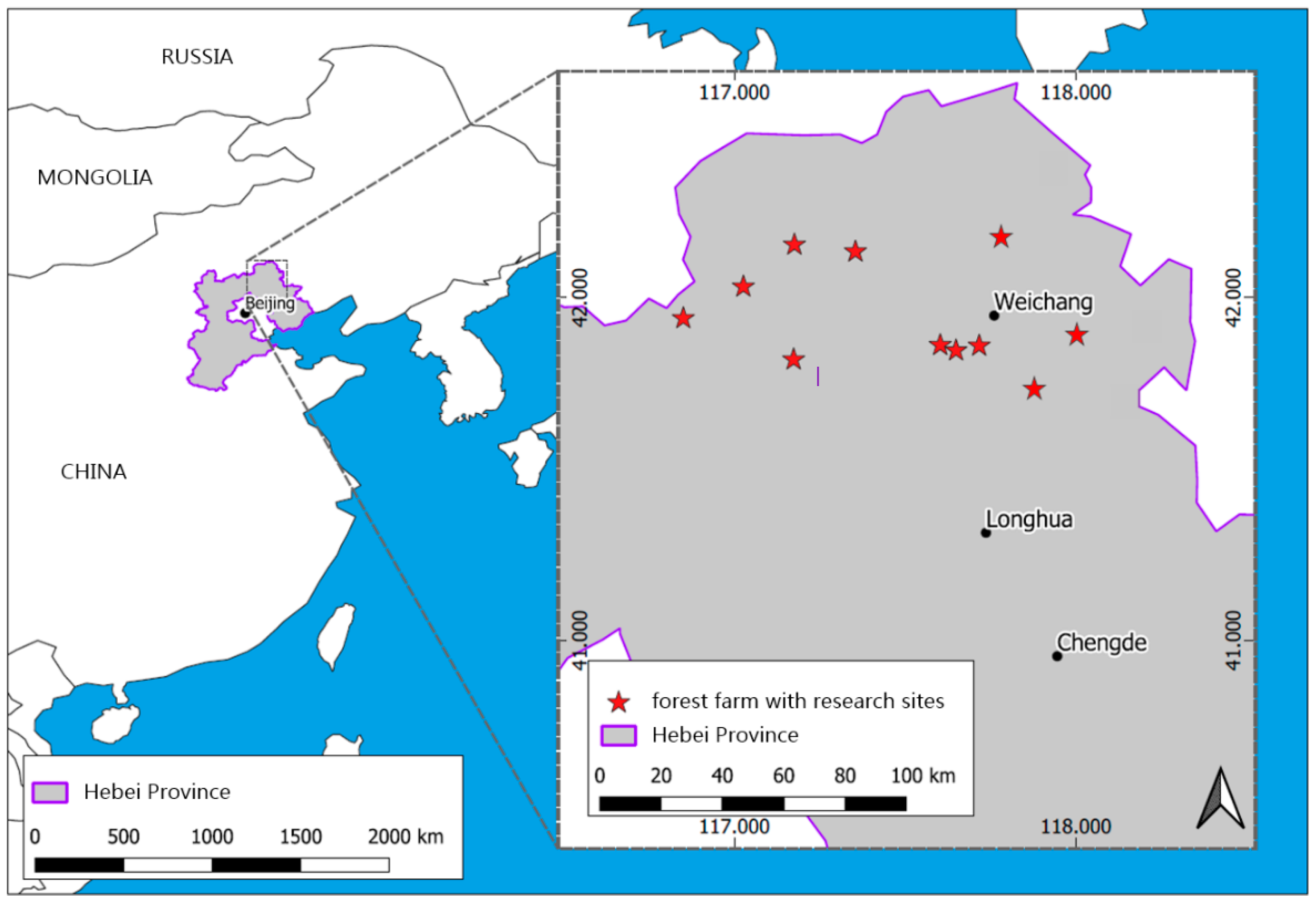
The research sites are situated in the Mulan Weichang State-Owned Forest Farm (hereinafter referred to as Mulan Forest) in Weichang County of Hebei Province in Northeast China (41°35′–42°40′ N, 116°32′–117°94′ E) with Inner Mongolia lying to the north and Beijing and Tianjin lying to the south (Figure 1). The territories of Mulan Forest are divided into 90,100 ha of closed forest land area, including 50,200 ha of public welfare forest, 39,900 ha of commercial forest and 667 ha of special use forest. The young forests (age ≤ 20) in Mulan Forest make up an area of 27,333 ha, the middle-aged forests (age 21–30) of 26,667 ha, the near-mature forests (age 31–40) of 20,667 ha, the mature forests (age 41–60) of 11,333 ha and the over-mature forests (age > 61) of 4100 ha [32].

A mid-temperate climate prevails in this province, which is defined as a hot and semi-humid summer and a cold and dry winter. The mean annual air temperature is 5.1 °C with a maximum of 21.0 °C in July and a minimum of −12.8 °C in January. The frost-free period encompasses 128 to 210 days a year. The total annual precipitation for the monitoring period 1951 to 2013 ranges from 240 mm to 680 mm. Due to the East Asian Summer Monsoon (EASM), around 70 % of the annual precipitation falls in the period from July to August with a peak of 130 mm in July (meteorological station of Weichang County, Hebei province, 1951–2013). The predominant forest type in this area is the temperate coniferous forest dominated by the tree species Pinus tabuliformis Carr. The elevation ranges from 950 to 1750 m a.s.l. and the topography is slightly hilly [4].

Since no site mapping has been performed for this region so far, the selection of the investigation stands is based on data acquired by the last forest inventory, which took place in 2014 (extracted from the forest inventory of Mulan Forest). The measured growth data of top height and tree age offered valuable clues to a provisional relative classification of the sites in “high”, “medium” and “low” productivity, using site index (SI) as a proxy for site productivity [1].

In order to exclude inter-specific competition, even-aged monocultures and well-stocked stands with relatively low-intensity management regimes were preferably selected. Since growth data of mature trees provide relevant information about long-term tree growth, the selected forest stands were as old as possible to maximize the observation period. According to the sampling design, nine research stands with 27 to 30 dominant individuals per tree species were selected for the three site productivity classes (

Table 2. Number of stands, trees, stem discs and annual shoot length measurements for each tree species and range of values, mean and standard deviation for tree age (yr) and tree height (m).

Tree Species	Stands	Trees	Stem Discs	Annual Shoot Length Measurements	Tree Age			Tree Height
					Range	Mean	SD	Range	Mean	SD
L. gmelinii	9	30	232	1308	39–98	69	20.6	12.7–30.6	21.7	7.2
P. tabuliformis	9	30	215	1529	41–108	75	22.4	10.3–24.7	17.5	4.9
P. sylvestris	9	27	184	725	24–40	32	3.5	11.6–18.6	15.1	2.5
P. asperata	9	30	235	1007	28–104	66	26.2	10.8–27.7	19.3	5.1
Q. mongolica	9	30	313	30	38–100	69	9.9	7.4–16.8	12.1	2.7
B. platyphylla	9	29	310	1308	38–96	67	14.7	11.9–25.5	18.7	4.2
B. dahurica	9	27	206	1529	39–70	55	8.1	9.1–19.2	14.2	2.6
P. davidiana	9	30	339	725	32–72	52	13.5	19.4–29.3	24.4	2.6

). As the stand height curve of dominant trees in the analyzed old, even-aged stands is rather flat the height of dominant trees can be used as measure for the 100 largest trees per ha. Assuming height growth differences on slopy terrain, a sample of three dominant trees at top, middle and lower slope was selected. In plain areas three samples of three dominant trees were identified. In addition, at each sample point height and diameter of ten dominant trees were measured, but only the three most dominant trees were cut for height growth analysis.

2.3. Characteristics of the Sample Trees for Height Growth Analysis

Exclusively dominant trees according to Kraft classes one and two [33] were selected for stem disc collection and shoot length measurement, as their growth is least affected by silvicultural measures. Furthermore, they are the most stable height-based indicators of site productivity [34]. Nevertheless, environmental conditions in the surrounding forest, e.g., the wind-sheltering effect of adjacent stands and practical aspects of forest operations, like soil compaction, may influence the height growth potential of the dominant trees. The sample trees were chosen in closed canopy surroundings, in order to reduce effects of gaps, skid trails or admixed tree species in the direct neighborhood. Sample trees should also have a healthy crown and no deterioration by felling or skidding damage. Some stem discs could not be measured because they were broken or could not be analyzed for other reasons. A small number of trees had to be excluded from further analysis because of irregular growth caused by suppression or damages, which were not visible when the sample trees were selected. A description of the selected stands and trees is provided in Table 2.

2.4. Field and Laboratory Measurements

Height of the sample trees was measured using a digital clinometer (Forester Vertex type III) and diameter at breast height using a diameter tape. Tree height measurements were recorded to an accuracy of 0.1 m and tree diameters to 0.1 cm. Sectioning was carried out by cutting discs at the base of the tree (0.3 m), at breast height (1.3 m), at a height of 3.0 m and 5.0 m and above 5.0 m at 3.0 m intervals for the conifers along the stem. Similarly, on felled broadleaved trees boles were cut at heights of 0.3 m, 1.3 m, 3.0 m, 4.0 m, 5.0 m, 7.5 m, 8.75 m, 10.0 m and approximately 1.25 m intervals subsequently. All stem discs were coded [35,36].

In addition, the annual shoot length was measured [1] by identifying the scar of the terminal bud scales following standard procedures outlined in Roloff [37]. While the scars of the bud scales of conifers were easily retraced for 30 to 40 years, the scars of broadleaved trees, especially of oaks, were difficult to identify. Here, you have to differentiate between “real” scars, which arise from annual shoots, or “false” scars, which arise from second flushes within a year, called regrowth or secondary growth [38]. In these cases, stem discs were taken up to the crown in small intervals to determine the annual height growth based on tree-rings. Sampling took place during the growing season of year 2014.

All discs were first air-dried, sanded with an orbital sander and then scanned (ScanMaker 9800XL plus, Microtek (Hsinchu, Taiwan)). For crossdating the tree-rings, the scanned images were imported in ‘WinDendro^TM’ [39]. Tree-rings were calculated from the quadratic mean of eight radii per stem disc. Automatic measurements generated by the software were inspected and manually corrected if necessary.

The tree-ring data has been quality checked and processed together with the annual shoot length measurements using the ‘height analysis’ software developed at the Chair of Forest Growth and Dendroecology at Albert-Ludwigs-University Freiburg, Germany. The program automatically checks the tree-rings between two stem discs for completeness and, if necessary, corrections can be performed manually.

To correct irregularities in growth of young trees caused by browsing damage or snow pressure, it was assumed that the trees reach 0.3 m three years after germination. The time for reaching 1.3 m is calculated by the median number of annual rings between the 0.3 m and the 1.3 m disc for each tree species.

2.5. Statistical Analysis Methods

All statistical analyses were performed in R version 4.0.2 using R Studio [40,41].

2.5.1. Model Development

The algebraic difference approach (ADA) was developed by Bailey and Clutter [14] and subsequently used as the basis for the generalized algebraic difference approach (GADA) developed by Cieszewski and Bailey [15]. Both techniques convert static age-height curves (base models) of the form

$$h=f\left(t|\alpha \right)$$

(1)

where h and t is a pair of height and age values and α is a vector of parameters, into dynamic age-height models. Therefore, both methods are used for site quality assessment as they provide more parsimonious, robust and base-age invariant results than static and base-age specific models [15,21]. In contrast to the ADA method, where only one site-specific parameter is replaced with a solution derived from the analyzed model, in the GADA model any desired number of parameters in the base growth model can be made site-specific by using an unobservable theoretical site variable X [15].

Solving the base model for X using known initial h and t values ($h_0$, $t_0$) and replacing parameters in the original equation, gives the ADA and GADA models the general implicit form

$$h_1=f\left(h_0, t_0, t_1|\beta \right)$$

(2)

where $h_1$ is the predicted height (in m) at age $t_1$ (in years), $h_0$ is the height at a reference age $t_0$ and β is a vector of global parameter estimates that results from the rearrangement of α [16].

Due to the short time series of our data, it was complicable to identify the most appropriate base models for our data material. We therefore tested GADA formulations of previously used base-age invariant growth models, against the data considered in this work and finally three models of exponential form (Chapman–Richards, Sloboda, Korf) and one of fractional form (Hossfeld) were selected based on their performance (

Table 3. Base models and generalized algebraic difference models (GADA) fitted to top height time series. $a_1$ $a_2$, $a_3$ and $a_4$ are parameters in the base model; $b_1, b_2$, and $b_3$ are parameters in the GADA models; $h_0$ and $h_1$ are heights (in m) at age $t_0$ and $t_1$ (in years); $X_0$ is the solution for X with initial values of height ($h_0$) and age ($t_0$). Detailed derivation of the models are given by Cieszewski and Bailey [15].

Base Model	Site-Specific Parameters	Solution for Variable X with Initial Values $({\mathit{h}}_0$$, {\mathit{t}}_0)$	GADA Model Form	Tree Species
Chapman–Richards [45]: $h=a_1{\left(1-e^{-a_{2}t}\right)}^{a_3}$	$a_1$= X	$X_0$= $\frac{h_0}{{\left(1-e^{-b_1{t}_0}\right)}^{b_2}}$	Krumland and Eng [12] in Sharma [17]: $h_1=h_0{\left(\frac{1-e^{-b_1{t}_1}}{1-e^{-b_1{t}_0}}\right)}^{b_2}$	P. asperata P. davidiana	[I]
	$a_1=e^X$ $a_3=b_2+\frac{b_3}{X}$	$X_0$=$\frac{1}{2}\left(\psi +\sqrt{{\psi }^2-4b_3\phi }\right)$ with$\psi$ = ln$h_0-b_2\phi$ and$\phi =ln\left(1-e^{-b_1{t}_0}\right)$	Krumland and Eng [12] in Sharma [17]: $h_1$= $h_0{\left(\frac{1-e^{-b_1{t}_1}}{1-e^{-b_1{t}_0}}\right)}^{\left(b_2+\frac{b_3}{X_0}\right)}$	P. tabuliformis P. sylvestris B. dahurica	[II]
Hossfeld [46]: $h=\frac{a_1}{1+a_2{t}^{-a_3}}$	$a_2$= X	$X_0$= $t_0^{b_3}\left(\frac{b_1}{h_0}-1\right)$	Anta et al. [47] in Sharma [17]: $h_1$=$\frac{b_1}{\left(1-\left(1-\frac{b_1}{h_0}\right){\left(\frac{t_0}{t_1}\right)}^{b_3}\right)}$	L. gmelinii	[III]
Sloboda [48]: h = $a_1{e}^{-a_2 e^{\left(\frac{a_3 }{\left(a_4-1\right)t^{\left(a_4-1\right)}}\right)}}$	$a_2$ = X	$X_0$ = $-\frac{ln\left(\frac{h_0}{b_1}\right)}{e^{\left(\frac{b_2}{\left(b_3-1\right)t_0{}^{\left(b_3-1\right)}}\right)}}$	Anta and Dieguez-Aranda [49] in Sharma [17]: $h_1=b_1{\left(\frac{h_0}{b_1}\right)}^{e^{\left(\frac{b_2}{\left(b_3-1\right)t_1{}^{\left(b_3-1\right)}}-\frac{b_2}{\left(b_3-1\right)t_0{}^{\left(b_3-1\right)}}\right)}}$	Q. mongolica	[IV]
Korf [50]: $h=a_1{e}^{\left(-a_2{t}^{-a_3}\right)}$	$a_1=e^X$ $a_3=\frac{\left(b_1+b_2\right)}{X}$	$X_0$= $\frac{1}{2}{t}_0^{-b_3}\left(\psi +\sqrt{4b_2{t}_0^{b_3}+{\left(-\psi \right)}^2}\right)$ with$\psi =b_1+t_0^{b_3}ln{h}_0$	Anta et al. [47] in Sharma [17]: $h_1=e^{X_0}{e}^{\left(-\left(\frac{b_1+b_2}{X_0}\right)t_1^{-b_3}\right)}$	B. platyphylla	[V]

):

Two GADA formulations of the Chapman–Richards model [I,II] for P. asperata, P. davidiana, P. tabuliformis, P. sylvestris and B. dahurica, one GADA formulation of the Hossfeld model [III] for L. gmelinii, one GADA formulation of the Sloboda model [IV] for Q. mongolica and one GADA formulation of the Korf model [V] for B. platyphylla.

2.5.2. Model Calibration and Evaluation

Autocorrelated residuals are expected because the database contains multiple observations within each individual tree and multiple trees within the same stand. To accommodate the potential correlation between subsequent measurements due to temporally and spatially nested data a first order autoregressive AR (1) error structure has been applied.

$${\epsilon }_i={\rho }^{t_i-t_{i-1}}{\epsilon }_{i-1}+{\alpha }_{i }$$

(3)

where ${\epsilon }_i$ is the ordinary residual of the ith measurement, ρ is the autoregressive parameter to be estimated, $t_i-t_{i-1}$ is the time distance between two observations and ${\alpha }_{i }$ is the independent and identically distributed error with ${\alpha }_{i }$∼ N(0, σ) [22,42].

The model parameters were estimated with nonlinear least squares regression. We used the function nlxb of the R package nlmrt, which attempts to find the minimum of the nonlinear sum of squares by using a variant of Marquardt’s approach to stabilize the Gauss-Newton method with the Levenberg-Marquardt adjustment [43]. The site-specific parameters (specific for each individual) and the global model parameters (shared by all individuals) were estimated simultaneously using nested regression techniques [12,13,15] and the following iterative procedure [12,17]:

(1)

Estimation of the global parameters

(2)

Estimation of the site-specific parameter using the estimates of the global parameters in step (1)

(3)

Re-estimation of the global parameters using the site-specific parameter estimates in step (2)

(4)

Iteration of the steps (2) and (3) until the residual sums of squares from successive iterations stabilizes.

The estimation of the autoregressive parameter ρ takes place simultaneously with the other parameters in the nested regression.

The performance of the five models was evaluated using the following fit statistics: (4) adjusted coefficient of determination (${\mathrm{R}}_{\mathrm{adj}}^2$), which shows the proportion of the total variance that is explained by the model, adjusted for the number of model parameters and the number of observations, (5) root mean square error of residuals (RMSE), which analyses the accuracy of the estimates and (6) the absolute average bias (AAB), which tests the systematic deviation of the model from the observations. The formulas are:

$$R_{adj}^2=1-\left(\frac{\left(n-1\right){{\displaystyle \sum }}_{i=1}^n{\left(y_i-{ŷ}_i\right)}^2}{\left(n-p\right){{\displaystyle \sum }}_{i=1}^n{\left(y_i-{\overline{y}}_i\right)}^2}\right)$$

(4)

$$\mathit{RMSE}=\sqrt{\frac{{{\displaystyle \sum }}_{i=1}^n{\left(y_i-{ŷ}_i\right)}^2}{n-p}}$$

(5)

$$AAB=\frac{1}{n}{\displaystyle \sum }_{i=1}^n\left(y_i-{ŷ}_i\right)$$

(6)

where p is the number of model parameters, n is the number of observations and $y_i$,${\overline{y}}_i, {ŷ}_i$ are the observed, average and predicted values of top height, respectively.

In addition, the modeled top height growth curves were compared with the trajectories of the observed heights and each model’s distribution of residuals was analyzed to detect any pattern of dependence or heteroscedasticity. A visual assessment of the models’ behavior outside the range of the modeled values was carried out, as well.

To estimate site quality from any given pair of height and age requires the selection of a reference age to which the top height growth will be referred to. According to Goelz and Burk [44] the reference age should be close to the rotation age and it should be a reliable predictor of height at other ages. In our study a reference age of 30 years was chosen to provide the possibility of site assessment for even rather young stands. Depending on the tree species five to seven top height growth curves were generated, with top heights between 3 m and 22 m.

3. Results

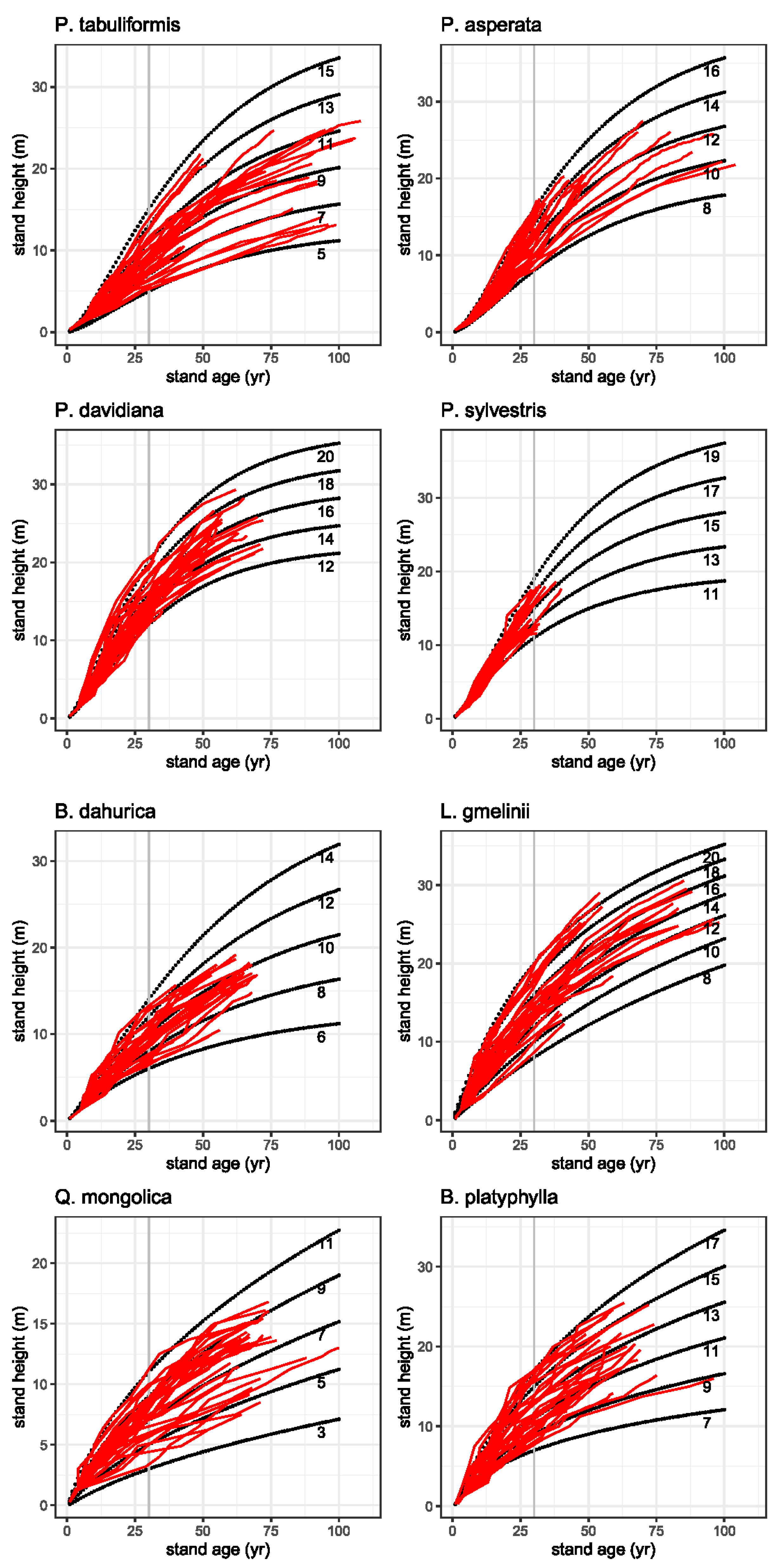
The observed height growth and the modeled top height growth curves at reference age 30 are shown in Figure 2. One striking feature is the decidedly different height growth pattern among the two pine species. On the high productivity sites P. sylvestris reaches heights of 12 m after 20 years and 18 m after 30 years. P. tabuliformis in comparison shows a lower height growth on the high productivity sites. This species reaches heights of 18 m only at an age of 40 to 45 years. At an age of 30, P. tabuliformis reaches a maximum height of 14 m. The heights of L. gmelinii at age 30 varies between 9 m and 20 m and the growth pattern of P. asperata reveals heights between 8 m and 16 m at the reference age. All conifers show a relatively uniform growth pattern compared to the hardwood species showing a more heterogeneous pattern. We found for Q. mongolica a relatively slow height growth in early years with maximum 11 m at age 30. Comparing the growth patterns of the two birch species, B. platyphylla shows a faster height growth than B. dahurica. On the high productivity sites B. platyphylla reaches heights of up to 17 m in 30 years, while B. dahurica reaches maximum heights of 13 m at the same age.

Trees on very good sites have a very rapid increase in early height growth in contrast to trees on poorer sites, which have much slower early height growth. The graphical inspection of the modeled top height growth curves showed a realistic progression, as they followed the measured trajectories of top height growth and did not cross them (Figure 2).

The parameter estimates for each top height growth model and their goodness-of-fit statistics are shown in

Table 4. Estimated parameters for the GADA models and goodness-of-fit statistics: RMSE = root mean square error (m); ${\mathrm{R}}_{\mathrm{adj}}^2$ = adjusted R²; AAB = average absolute bias (m).

Parameter Estimates						Fit Statistics
Tree Species	Parameter	Estimate	SE	t-Value	Pr (>|t|)	RMSE	$R_{adj}^2$	AAB
L. gmelinii	b1	51.772	3.0440	17.01	<0.001	0.5979	0.9956	0.3883
	b3	1.0118	0.0266	38.06	<0.001
P. tabuliformis	b1	0.0139	0.0002	92.83	<0.001	0.3792	0.9966	0.1928
	b2	1.9426	0.0368	52.73	<0.001
	b3	−2.7807	0.1179	−23.58	<0.001
P. sylvestris	b1	0.0306	0.0004	83.33	<0.001	0.3024	0.9960	0.1685
	b2	2.8043	0.1584	17.71	<0.001
	b3	−4.9288	0.5274	−9.35	<0.001
P. asperata	b1	0.0273	0.0004	66.93	<0.001	0.3337	0.9979	0.2322
	b2	1.5622	0.0274	57.03	<0.001
Q. mongolica	b1	9.2465	0.3937	23.49	<0.001	0.4748	0.9889	0.3541
	b2	0.1204	0.0069	17.25	<0.001
	b3	1.0644	0.0049	213.90	<0.001
B. platyphylla	b1	10.4131	0.5222	19.94	<0.001	0.7628	0.9866	0.5737
	b2	−20.2949	2.3630	−8.59	<0.001
	b3	0.2994	0.0031	98.13	<0.001
B. dahurica	b1	0.0190	0.0004	43.30	<0.001	0.6877	0.9858	0.4996
	b2	1.9289	0.1149	16.79	<0.001
	b3	−2.5615	0.3602	−7.11	<0.001
P. davidiana	b1	0.0356	0.0008	43.82	<0.001	0.6925	0.9921	0.5267
	b2	1.4489	0.0389	37.19	<0.001

. All of the parameters were significantly lower than the α-level of 0.05. All models had quite similar goodness-of-fit statistics and explained more than 98% of the total variance in the fitting phase. The best performance showed P. asperata and P. tabuliformis with an average absolute bias (AAB) of 0.2322 m and 0.1928 m, root mean square errors (RMSE) of 0.3337 m and 0.3792 m and ${\mathrm{R}}_{\mathrm{adj}}^2$ of 0.9979 and 0.9966. B. dahurica achieved the worst results with AAB of 0.4996 m, RMSE of 0.6877 m and ${\mathrm{R}}_{\mathrm{adj}}^2$ of 0.9858. The determination of the model parameters by using repetitive procedures contribute significantly to the reduction of total dispersion in all tree species.

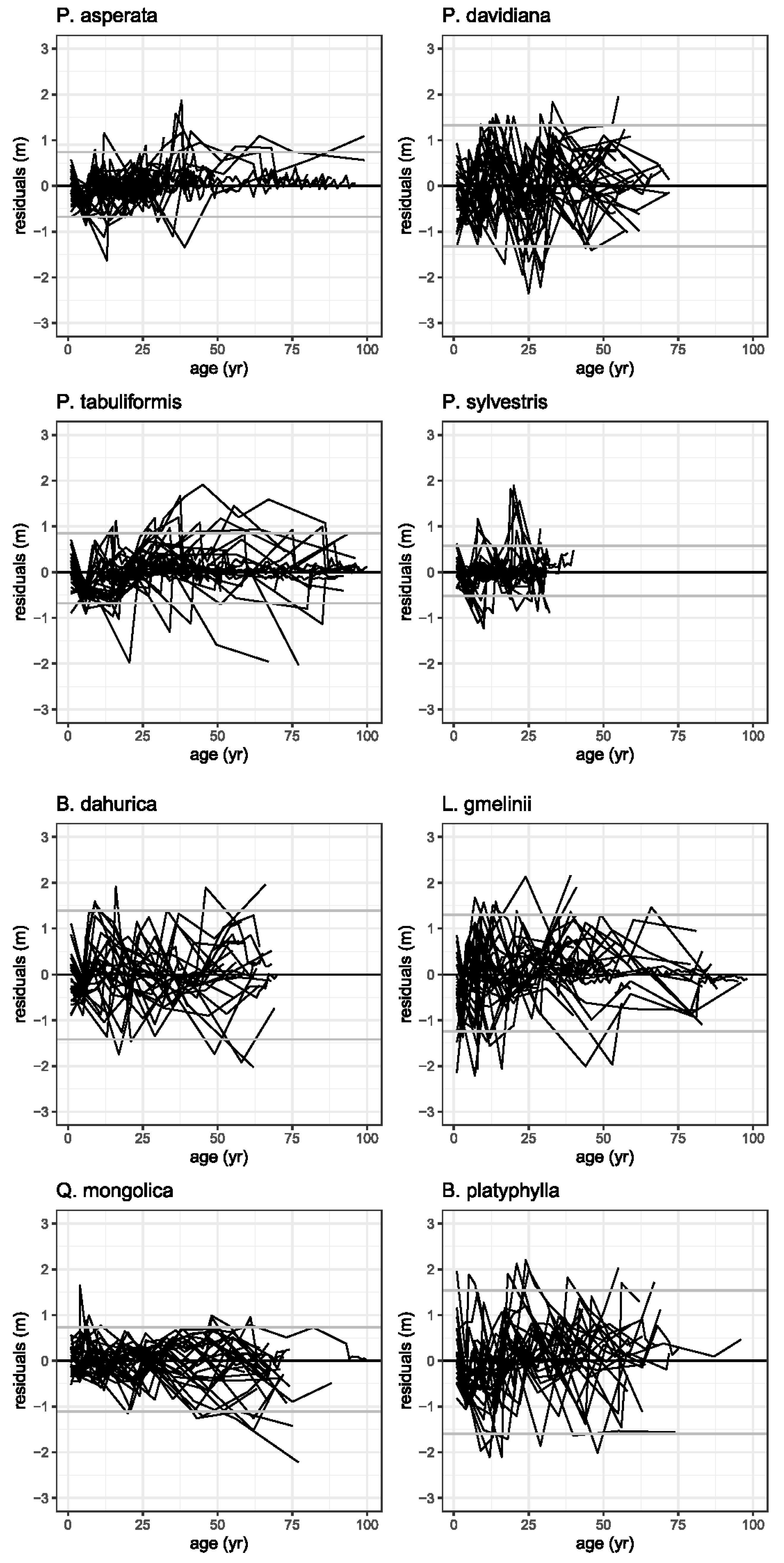
The distribution of the residuals versus tree age were scattered around 0 and without visible trends, indicating that the fitness of the models was good. The best results were obtained for P. asperata and P. sylvestris (Figure 3). No pattern was found in the residuals for any of the tree species and top height growth models.

4. Discussion

4.1. Development of Top Height Growth Models

In this study, we developed top height growth models for eight native Chinese tree species using the GADA approach, which leads to an accurate top height growth modeling due to the formulation of variable asymptotes. Our models are dynamic, so top heights for a given stand can be predicted at any time in future from a top height observation at a given reference age. Given the importance placed on top height as a proxy for site productivity, we believe that our growth models facilitate implementing sustainable forest management practices in Mulan Forest.

Several growth models for top height development have been tested for suitability: The top height growth curves of Cieszewski [20] model behaved illogically in extrapolations, since they showed no inflection point and the trees seemed to grow endlessly. For Schumacher’s model no significant parameter estimates could be found and Weibull’s model showed fitting problems at the beginning and the end of the height growth series. Since trees are generally very young in the research area, deviations from the growth pattern in the first ten years and the last five years are not acceptable.

The growth models of Chapman–Richards, Hossfeld, Korf and Sloboda were finally selected since they satisfy the general requirements of top height growth models [22,51,52]: (1) they represent parsimonious, dynamic site models, (2) the top height growth curves do not cross, so the site quality remains constant along a top height growth curve, (3) the parameters, which determine the shape, depend on tree species as well as on site conditions, (4) they show a sigmoid growth pattern (increasing function with an inflection point), (5) the distribution of residuals does not show any visible trends and (6) they show a logical behavior (height is zero at age zero and equal to site index at the reference age).

Especially the Chapman–Richards and the Hossfeld age-height models are among the most successful models to describe growth in forestry [53] and have been used to construct top height growth models in a number of other studies [17,22,51,54].

4.2. Limitations of the Developed Top Height Growth Models

The derivation of top height growth models in our study is based on height growth analysis. Due to the lack of long-term experimental plots the study had to resort to retrospective height growth analysis and there remains a degree of uncertainty about the accuracy of the underlying data, particularly for old stands due to limited data availability. Whether the top height growth curves generated in this study would be followed throughout rotation can be validated with data from permanent plots. This entails establishing permanent sample plots in the study area, from which data would be collected over a period of time and used to validate these curves.

The development of top height growth curves generally assumes constant growing conditions [7]. Since the possibility cannot be ruled out that growth conditions have changed in recent decades, this can lead to misjudgments of future growth. Variations in site productivity for a given site have also been reported in several European countries [55,56,57]. These studies showed a higher site productivity for younger stands than for older stands under similar conditions caused by improved forest management practices over time [40]. If a site keeps changing, these curves need to be continuously updated with new data [7].

The development of top height growth curves places high demands on the quality of the underlying data. They should represent the growth characteristics of the local tree species and respective site conditions within the given age range [1,2,7]. The accuracy of the predicted top height growth curves increases with the age of the analyzed trees, since older trees provide a larger data volume than younger trees [1,2,7]. However, it should be noted that Chinese stands are rather young and with increasing age, deviations of the observed growth patterns from the modeled curves may occur due to the limited availability of data from old trees.

In Germany the reference age is normally set to 100 years for better comparability [7]. Several studies from other countries chose a significantly lower reference age, i.e., 20 years for Pinus caribaea var. hondurensis in the Dominican Republic [58], 50 years for Fagus sylvatica L. in Denmark [22] and upland oaks in the Central States [59] or even only 15 years for Pinus pseudostrobus Lindl. in Mexico [60]. However, in our case the scarcity of data at older ages advises against using a reference age older than 30 years. The reference age of 30 years used to create a family of top height growth curves is not optimal having in mind that reference age is usually chosen close to the rotation age. However, the rotation age of the respective tree species in China is between 15 and 40 years and therefore currently rather short [61]. In terms of representativeness, it is desirable that the period of rapid growth of all investigated tree species has passed and the culmination point of the mean annual height increment (MAI) is reached.

Despite the limitations mentioned, top height growth curves as models of forest growth in forest practice are highly versatile. They facilitate the understanding of complex growth processes in stands and are a practical resource for forest planning [1,2,7]. They can be used for determining top height growth and for estimating height and volume growth. However, such curves are always simplified models which do not reflect reality in all aspects. They reflect mean values, which may differ from those in specific stands. Despite these reservations, top height growth curves are an indispensable tool, in particular for increment estimation and for the formulation of sustainable forest management plans, especially silvicultural decision-making processes such as time and volume of first and subsequent thinnings.

5. Conclusions

For the eight Chinese tree species Larix gmelinii var. principis-rupprechtii., Pinus tabuliformis Carr., Pinus sylvestris var. mongolica Litv., Picea asperata Mast., Quercus mongolica Fisch. ex Ledeb, Betula platyphylla Suk., Betula dahurica Pall. and Populus davidiana Dode top height growth models have been developed. These models proofed to fit well to the observed values with ${\mathrm{R}}_{\mathrm{adj}}^2$ between 0.98 and 0.99 for all tree species. Based on our results, we conclude that the developed top height growth models, despite their short time series will be useful in identifying suitable sites for the investigated tree species and to quantify and predict their growth and yield on various site conditions. They facilitate the understanding of complex growth processes in even-aged homogenous stands and are useful tools for forest managers for various purposes such as inventory updating, evaluation of silvicultural alternatives and harvest scheduling. As soon as large representative samples of permanent plots are available and forest site mapping has been performed for the research area, the top height growth curves have to be adjusted to the new data [8].

References

- Skovsgaard, J.P.; Vanclay, J.K. Forest site productivity: A review of the evolution of dendrometric concepts for even-aged stands. Forestry 2008, 81, 12–31. [Google Scholar] [CrossRef] [Green Version]
- Pretzsch, H. Grundlagen der Waldwachstumsforschung; Springer: Berlin/Heidelberg, Germany, 2017; p. 664. ISBN 978-3-662-58155-1. [Google Scholar] [CrossRef]
- Pretzsch, H. Modellierung des Waldwachstums; Parey: Singhofen, Germany, 2003; p. 341. ISBN 978-3-8001-4555-3. [Google Scholar]
- Dai, L.; Wang, Y.; Su, D.; Zhou, L.; Yu, D.; Lewis, B.J.; Qi, L. Major forest types and the evolution of sustainable forestry in China. Environ. Manag. 2011, 48, 1066–1078. [Google Scholar] [CrossRef]
- Xu, H.; Sun, Y.; Wang, X.; Fu, Y.; Dong, Y.; Li, Y. Nonlinear Mixed-Effects (NLME) Diameter Growth Models for Individual China-Fir (Cunnighamia lanceolata) Trees in Southeast China. PLoS ONE 2014, 9, e104012. [Google Scholar] [CrossRef]
- Bachmann, P. Skript Waldwachstum. Professur für Forsteinrichtung und Waldwachstum ETH Zürich. 2008. Available online: https://www.wsl.ch/forest/waldman/vorlesung/ww_tk62.ehtml (accessed on 20 January 2021).
- Assmann, E.; Franz, F. Vorläufige Fichtenertragstafeln für Bayern. In Hilfstafeln für die Forsteinrichtung, Auflage 1990; Institut für Ertragskunde der Forstlichen Forschungsanstalt: München, Germany, 1963; pp. 52–63. [Google Scholar]
- Kindermann, G. Methoden zur Erstellung von Oberhöhenfächern. In Tagungsbericht 2015 der Sektion Ertragskunde (DVFFA), Deutscher Verband Forstlicher Forschungsanstalten, Kohnle, U.; Klädtke, J., Ed.; Sektion Ertragskunde der Forstlichen Versuchs- und Forschungsanstalt Baden-Württemberg: Freiburg, Germany, 2015; pp. 143–152. [Google Scholar]
- Wiedemann, E. Ertragstafeln der Wichtigen Holzarten bei Verschiedener Durchforstung Sowie Einiger Mischbestandsformen; M. & H. Schaper: Hannover, Germany, 1949; 100p. [Google Scholar]
- von Gadow, K. Waldstruktur und Wachstum; Universitätsverlag: Göttingen, Germany, 2003; p. 254. ISBN 3-930457-32-6. [Google Scholar]
- Sánchez-González, M.; Stiti, B.; Chaar, H.; Cañellas, I. Dynamic dominant height growth model for Spanish and Tunisian cork oak (Quercus suber L.) forest. For. Syst. 2010, 19, 285–298. [Google Scholar] [CrossRef]
- Krumland, B.; Eng, H. Site index systems for major young-growth forest and woodland species in northern California. California Department of Forestry and Fire Protection, Sacramento, CA. Calif. For. Rep. 2005, 4, 1–219. [Google Scholar]
- Cieszewski, C.J.; Strub, M.; Zasada, M. New dynamic site equation that fits best the Schwappach data for Scots pine (Pinus sylvestris L.) in Central Europe. For. Ecol. Manag. 2007, 243, 83–93. [Google Scholar] [CrossRef]
- Bailey, R.L.; Clutter, J.L. Base-age invariant polymorphic site curves. For. Sci. 1974, 20, 155–159. [Google Scholar] [CrossRef]
- Cieszewski, C.J.; Bailey, R.L. generalized algebraic difference approach: Theory Based Derivation of Dynamic Site Equations with Polymorphism and Variable Asymptotes. For. Sci. 2000, 46, 116–126. [Google Scholar]
- Manso, R.; McLean, J.P.; Arcangeli, C.; Matthews, R. Dynamic top height models for several major forest tree species in Great Britain. Forestry 2021, 94, 181–192. [Google Scholar] [CrossRef]
- Sharma, R.P.; Brunner, A.; Eid, T.; Oyen, B.-H. Modelling dominant height growth from national forest inventory individual tree data with short time series and large age errors. For. Ecol. Manag. 2011, 262, 2162–2175. [Google Scholar] [CrossRef]
- Ercanli, I.; Kahriman, A.; Yavuz, H. Dynamic base-age invariant site index models based on generalized algebraic difference approach for mixed Scots pine (Pinus sylvestris L.) and Oriental beech (Fagus orientalis Lipsky) stands. Turk J. Agric. For. 2014, 38, 134–147. [Google Scholar] [CrossRef]
- Akbas, U.; Senyurt, M. Site quality estimations based on the generalized algebraic difference approach: A case study in Cankiri forests. Rev. Arvore 2018, 42, 1–10. [Google Scholar] [CrossRef] [Green Version]
- Cieszewski, C.J. Three methods of deriving advanced dynamic site equations demonstrated on inland Douglas-fir site curves. Can. J. For. Res. 2001, 31, 165–173. [Google Scholar] [CrossRef]
- Cieszewski, C.J. Comparing Fixed- and Variable-Base-Age Site Equations Having Single Versus Multiple Asymptotes. For. Sci. 2002, 48, 7–23. [Google Scholar]
- Nord-Larsen, T. Developing dynamic site index curves for European beech (Fagus sylvatica L.) in Denmark. For. Sci. 2006, 52, 173–181. [Google Scholar]
- Farjon, A. Pinus tabuliformis. In The IUCN Red List of Threatened Species; IUCN Red List: Gland, Switzerland, 2013; p. e.T42419A2978916. [Google Scholar] [CrossRef]
- Liu, B.; Bussmann, R.W. Pinus sylvestris L. var. mongolica Litv. Pinaceae. In Ethnobotany of the Mountain Regions of Central Asia and Altai; Batsatsashvili, K., Kikvidze, Z., Bussmann, R., Ethnobotany of Mountain Regions, Eds.; Springer: Cham, Germany, 2020; pp. 1–8. [Google Scholar] [CrossRef]
- Farjon, A. Larix gmelinii var. Principis-rupprechtii. In The IUCN Red List of Threatened Species; IUCN Red List: Gland, Switzerland, 2013; p. e.T191616A1991224. [Google Scholar] [CrossRef]
- Carter, G.; Farjon, A. Picea asperata. In The IUCN Red List of Threatened Species; IUCN Red List: Gland, Switzerland, 2013; p. e.T42320A2972242. [Google Scholar] [CrossRef]
- Barstow, M. Quercus mongolica. In The IUCN Red List of Threatened Species; IUCN Red List: Gland, Switzerland, 2018; p. e.T194200A2303793. [Google Scholar] [CrossRef]
- Gradel, A.; Haensch, C.; Batsaikhan, G.; Batdorj, D.; Ochirragchaa, N.; Günther, B. Response of white birch (Betula platyphylla Sukaczev) to temperature and precipitation in the mountain forest steppe and taiga of northern Mongolia. Dendrochronologia 2017, 41, 24–33. [Google Scholar] [CrossRef]
- Hua, H. Betula dahurica Pal. In Flora of China; Science Press: Beijing, China, 2002; Volume 4, p. 312. [Google Scholar]
- Hou, Z.; Li, A.; Zhang, J. Genetic architecture, demographic history, and genomic differentiation of Populus davidiana revealed by whole-genome resequencing. Evol. Appl. 2020, 13, 2582–2596. [Google Scholar] [CrossRef]
- Ni, J.; Zhang, X.-S.; Scurlock, J.M.O. Synthesis and analysis of biomass and net primary productivity in Chinese forests. Ann. For. Sci. 2001, 58, 351–384. [Google Scholar] [CrossRef]
- Hu, X.; (Chinese Academy of Forestry, Beijing, China). Personal communication, 2014.
- Kraft, G. Beiträge zur Lehre von den Durchforstungen, Schlagstellungen und Lichtungshieben; Klindworth: Hannover, Germany, 1884; p. 147. [Google Scholar]
- West, P.W. Tree and Forest Measurement, 3rd ed.; Springer International Publishing: Basel, Switzerland, 2015; p. 214. [Google Scholar]
- Van Laar, A.; Akca, A. Forest Mensuration; Springer: Heidelberg, Germany, 2007; p. 390. ISBN 13-978-1-4020-5991-9. [Google Scholar]
- Kramer, H.; Akca, A. Leitfaden zur Waldmesslehre; J.D. Sauerländer’s Verlag: Frankfurt, Germany, 2008; p. 226. ISBN 978-3-7939-0880-7. [Google Scholar]
- Roloff, A. Kronenentwicklung und Vitalitätsbeurteilung Ausgewählter Baumarten der Gemäßigten Breiten; J.D. Sauerländer’s Verlag: Frankfurt, Germany, 1994; p. 258. ISBN 978-3793950936. [Google Scholar]
- Huixun, Z.; Chuankuan, W.; Binhui, L. Growth of Mongolian Oak. J. Northeast For. Univ. 1994, 5, 10–17. [Google Scholar]
- WinDendroTM. Manual for Tree-Ring Analysis; Instruments Regent Inc.: Quebec, CA, USA, 2014; Available online: http://www.regentinstruments.com (accessed on 3 September 2020).
- R Core Team. R: A Language and Environment for Statistical Computing; R Foundation for Statistical Computing: Vienna, Austria, 2019. [Google Scholar]
- RStudio Team. RStudio: Integrated Development Environment for R; RStudio, Inc.: Boston, MA, USA, 2019. [Google Scholar]
- Hyndman, R.J.; Athanasopoulos, G. Forecasting: Principles and Practice, 2nd ed.; Monash University: Melbourne, Australia, 2018. [Google Scholar]
- Available online: https://cran.r-project.org/web/packages/nlmrt/nlmrt.pdf (accessed on 28 June 2021).
- Goelz, J.C.G.; Burk, T.E. Development of a well-behaved site index equation: Jack pine in north central Ontario. Can. J. For. Res. 1992, 22, 776–784. [Google Scholar] [CrossRef]
- Richards, F.J. A Flexible Growth Function for Empirical Use. J. Exp. Bot. 1959, 10, 290–300. [Google Scholar] [CrossRef]
- Hossfeld, J.W. Mathematik für Forstmänner, Ökonomen und Cameralisten. Gotha 1822, 4, 310. [Google Scholar]
- Anta, M.B.; Dorado, F.C.; Dieguez-Aranda, U.; Gonzalez, J.G.A.; Parresol, B.R.; Soalleiro, R.R. Development of a basal area growth system for maritime pine in northwestern Spain using the generalized algebraic difference approach. Can. J. For. Res. 2006, 36, 1461–1474. [Google Scholar] [CrossRef] [Green Version]
- Sloboda, B. Zur Darstellung von Wachstumsprozessen mit Hilfe von Differentialgleichungen erster Ordnung. In Mitteilungen der Forstlichen Versuchs- und Forschungsanstalt Baden-Württemberg; Forstliche Versuchs- und Forschungsanstalt Baden-Württemberg: Freiburg, Germany, 1971; Volume 32, p. 109. [Google Scholar]
- Anta, M.B.; Dieguez-Aranda, U. Site quality of pedunculate oak (Quercus robur L.) stands in Galicia (northwest Spain). Eur. J. For. Res. 2005, 124, 19–28. [Google Scholar] [CrossRef]
- Korf, V. Pøíspìvek k matematické definici vzrùstového zákona lesních porostù. Lesnická Práce 1939, 18, 339–356. [Google Scholar]
- Liziniewicz, M.; Nilsson, U.; Agestam, E.; Ekö, P.M.; Elfving, B. A site index model for lodgepole pine (Pinus contorta Dougl. var. latifolia) in northern Sweden. Scand. J. For. Res. 2016, 31, 583–591. [Google Scholar] [CrossRef]
- Cieszewski, C.J. Developing a well-behaved dynamic site equation using a modified Hossfeld IV function Y−3 = (ax(m))/(c + x(m − 1)), a simplified mixed-model and scant subalpine fir data. For. Sci. 2003, 494, 539–554. [Google Scholar]
- Zeide, B. Analysis of growth equations. For. Sci. 1993, 39, 594–616. [Google Scholar] [CrossRef]
- Dieguez-Aranda, U.; Burkhart, H.E.; Rodriguez-Soalleiro, R. Modeling dominant height growth of radiata pine (Pinus radiata D. Don) plantations in north-western Spain. For. Ecol. Manag. 2005, 215, 271–284. [Google Scholar] [CrossRef]
- Hägglund, B.; Lundmark, J.E. Site estimation by means of site properties: Scots pine and Norway spruce in Sweden. Stud. For. Suec. 1977, 138, 1–38. [Google Scholar]
- Spiecker, H. Overview of recent growth trends in European forests. Water Air Soil Poll. 1999, 116, 33–46. [Google Scholar] [CrossRef]
- Spiecker, H.; Mielikäinen, K.; Köhl, M.; Skovsgaard, J.P. Growth Trends in European Forests; Springer: Berlin/Heidelberg, Germany, 1996; p. 372. ISBN 978-3-642-61178-0. [Google Scholar] [CrossRef]
- Körner, M. Erfassung und Modellierung des Wachstums der Karibischen Kiefer (Pinus caribaea var. hondurensis) in der Dominikanischen Republik. In Tagungsbericht 2013 der Sektion Ertragskunde (DVFFA), Deutscher Verband Forstlicher Forschungsanstalten; Kohnle, U., Klädtke, J., Eds.; Sektion Ertragskunde der Forstlichen Versuchs- und Forschungsanstalt Baden-Württemberg: Freiburg, Germany, 2013; pp. 146–153. [Google Scholar]
- Carmean, W.H. Site Index Curves For Black, White, Scarlet, and Chestnut Oaks in The Central States. North Central Forest Experiment Station, U.S. Department of Agriculture. (USDA) For. Serv. Res. Paper NC 1971, 62, 1–8. [Google Scholar]
- Méndez, M.G.; Cobos, F.C.; Barraza, G.Q.; Larreta, B.V.; Luna, J.A.N. Dominant height growth model for Pinus pseudostrobus Lindl. in Guerrero state. Rev. Mex. De Cienc. For. 2016, 7, 7–20. [Google Scholar]
- Mann, S. Forest Protection and Sustainable Forest Management in Germany and the P.R. China—A Comparative Assessment; Federal Agency for Nature Conservation: Bonn, Germany, 2012; p. 120. [Google Scholar]
Figure 1.
Geographic map with the location of the forest farms and the research sites in Mulan Forest (d-maps.com (accessed on 3 February 2021); modified).
Figure 2.
Productivity of forest sites classified by stand height (m) at a given stand age (years) represented on a top height growth scale (22 m, 20 m, … 5 m, 3 m) for each tree species. Modeled top height growth curves (dashed black lines) obtained using several growth models at a reference age of 30 years (grey line) overlaid on the trajectories of the observed top heights of the trees (red lines).
Figure 3.
Illustration of the residuals (m) for each tree species. The horizontal grey lines represent the 2.5th and the 97.5th percentiles of a standard normal distribution.