
Integrated Evaluation of Vegetation Drought Stress through Satellite Remote Sensing †


1
Space Research and Technology Institute of the Bulgarian Academy of Sciences, Acad. G. Bonchev Str. Bl. 1, 1113 Sofia, Bulgaria
2
Ministry of Environment and Water, Maria Luisa Blvd. 22, 1000 Sofia, Bulgaria
*
Author to whom correspondence should be addressed.
†
This paper is dedicated to the memory of Prof. Roumen Nedkov, a brilliant scientist, who thrived on helping and teaching others learn.
Forests 2021, 12(8), 974; https://0-doi-org.brum.beds.ac.uk/10.3390/f12080974
Submission received: 19 May 2021
/
Revised: 15 July 2021
/
Accepted: 15 July 2021
/
Published: 22 July 2021
(This article belongs to the Special Issue Remote Sensing Applications in Forests Inventory and Management)
Abstract
:In the coming decades, Bulgaria is expected to be affected by higher air temperatures and decreased precipitation, which will significantly increase the risk of droughts, forest ecosystem degradation and loss of ecosystem services (ES). Drought in terrestrial ecosystems is characterized by reduced water storage in soil and vegetation, affecting the function of landscapes and the ES they provide. An interdisciplinary assessment is required for an accurate evaluation of drought impact. In this study, we introduce an innovative, experimental methodology, incorporating remote sensing methods and a system approach to evaluate vegetation drought stress in complex systems (landscapes and ecosystems) which are influenced by various factors. The elevation and land cover type are key climate-forming factors which significantly impact the ecosystem’s and vegetation’s response to drought. Their influence cannot be sufficiently gauged by a traditional remote sensing-based drought index. Therefore, based on differences between the spectral reflectance of the individual natural land cover types, in a near-optimal vegetation state and divided by elevation, we assigned coefficients for normalization. The coefficients for normalization by elevation and land cover type were introduced in order to facilitate the comparison of the drought stress effect on the ecosystems throughout a heterogeneous territory. The obtained drought coefficient (DC) shows patterns of temporal, spatial, and interspecific differences on the response of vegetation to drought stress. The accuracy of the methodology is examined by field measurements of spectral reflectance, statistical analysis and validation methods using spectral reflectance profiles.
1. Introduction
Drought is a part of the climate and can occur in any climate regime around the world [1]. A constant increase in extreme climate-related events has been observed, with a particularly sharp rise in the number of hydrological events [2,3]. This can have a direct effect on the frequency and intensity of droughts, leading to possible negative consequences for land-production systems [4].
Drought can arise from a range of hydro-meteorological processes that suppress precipitation and/or limit surface water or ground water availability, creating conditions that are significantly drier than normal [5]. The precipitation deficits generally appear initially as a deficiency in soil water [6]. It usually takes several weeks before precipitation deficiencies begin to produce soil moisture deficiencies that lead to stress on ecosystems.
Drought impacts different regions and climate zones around the world [7]. The analyses of drought variability during the last few decades show some regions with drying patterns in Europe. Situated in Southeastern Europe, Bulgaria is also subjected to the frequent short- and long-term droughts [8,9]. Increases in air temperatures and a reduction in precipitation in Bulgaria are expected within the next few decades [10], which will lead to higher transpiration and evapotranspiration values, especially in the summer seasons. This will significantly increase the risk of drought, loss of biodiversity and ES [11], and requires an accurate assessment of ecosystem responses to this phenomenon. The traditional approach for drought assessment evolved primarily from the meteorological and hydrological sciences. The introduction of interdisciplinarity and the application of the system approach divides drought into three main types—meteorological, blue-water, and green-water drought [12]. The green-water drought is expressed by reduced water storage in soil and vegetation. Green-water drought causes variable effects across landscape components, on their functioning and the ES they provide [12]. Blue-water, or irrigation water, is only required when the green-water store in the soil runs short [13]. Understanding drought-impact pathways across blue- and green-water fluxes and geospheres is crucial for ensuring food and water security and for developing early-warning and adaptation systems in support of ecosystems and society [14].
The distinct landscapes and the forest ecosystems [15] that developed on them react in different ways to the changes in the environmental conditions [16]. Application of indices and indicators based mainly on hydro-meteorological data cannot sufficiently achieve effective and accurate drought assessments. Similar disadvantages are also shown by remote sensing methodological approaches, based entirely on spectral vegetation indices [17]. Semi-natural ecosystems in lower territories wither earlier than those in higher areas. The application of a methodology for drought assessment that uses only spectral indices could lead to misinterpretation of this natural process, defining it as drought. In addition, the differences in the withering process and drought sensitivity of the individual land cover classes (LCCs) further superimpose the differences between the individual ecosystems and complicate the assessment of drought. The drought response of plant communities is also influenced by the within-ecosystem variability, predetermined by the differences in landscape-forming components such as the lithological basis, soil type, topography, and landscape hydrology. There is evidence that ecosystems respond more strongly to climate variability with decreasing climatic wetness and biomass [18,19], which suggests that the drought sensitivity would be greater in grasslands than in shrubs and, respectively, greater in shrubs than in forest ecosystems [17]. All these prerequisites require a methodology that takes into account the differences between the ecosystems and unifies the assessment of ecosystems’ drought response throughout a heterogeneous territory. Therefore, the present study introduces coefficients for the normalization of drought assessments by two key landscape-forming factors—elevation and land cover. The elevation is a dominant driver of drought sensitivity. In the high mountain areas, soil is shallow, with lower water retention capacity and consequently with reduced capacity to supply ecosystems with moisture under severe drought conditions. In the foothills and valleys, the soils are deeper, and the water retention capacity is greater. These areas are distinguished by shallow groundwater availability and provide better moisture supply to vegetation. Different LCCs are also characterized by various degrees of drought sensitivity. Studies on the gross primary productivity (GPP) changes of different land cover types under drought stress show, for example, a considerable reduction in the drought-induced GPP in the mid-latitude region of the northern hemisphere (48%), followed by the low-latitude region of the southern hemisphere (13%) [20]. In contrast, a slightly enhanced GPP (10%) was evident in the tropical region under drought impact [20]. Shrubs and grasslands have a lower biomass than forests and, under drought conditions, show stronger drought sensitivity and greater differential response to severe drought than to moderate drought [17,19]. Water-limited ecosystems, distinguished by low GPP, demonstrate a higher correlation between hydro-climate variation and vegetation greenness [18]. They respond with greater productivity decreases under drought stress [21], and show slower recovery after that [20].
The present study introduces an innovative, experimental methodology, which intends to assess the drought impact on semi-natural lands, including forest, shrub and grassland ecosystems. The application of the system approach, which takes into consideration key differences between the ecosystems and their functioning, is included as a necessary basis for accurate evaluation of the drought impact. The study outlines patterns of temporal, spatial, and interspecific differences in the response of vegetation to drought stress in a part of western Bulgaria, which is distinguished by its heterogeneity and diversity. These prerequisites make the study valuable for further drought-related research concerning various environments.
2. Materials and Methods
2.1. Study Area
The study area is located in western Bulgaria. It is representative of the areas with different vegetation (forests, shrubs, grass and pasture lands) which are considerably influenced by drought. The area covers two adjacent Sentinel-2 tile scenes, encompassing 17.2% of Bulgarian territory (Figure 1).
The local relief is diverse, including valleys, hilly areas and mountainous areas. The study area occupies parts of the Fore Balkan and Balkan Mountain Range, Vitosha Mountain, Sredna Gora and smaller adjacent mountains. The mean elevation is 715.5 m a.s.l. The highest point is 2277.6 m and the lowest is 83.4 m.
The climate is temperate-continental, characterized by relatively warm summers and cold winters. The mean annual temperatures vary between 10.3 °C in the lower areas and 0.3 °C at higher altitudes. The annual precipitation sum is between 610 and 1187 mm, depending on the elevation and slope exposure [22].
The main soil types include Luvisols, Cambisols, Leptosols, Planosols, Colluvisols, and Rendzinas. The valleys are characterized mainly by Fluvisols, whereas the high mountainous parts are characterized by Umbrisols. Within the area of the coniferous and beech forest spread, the Cambisols are predominant. In the low-latitude mountains and hilly areas, the soil types are more diverse, due to differences in the lithological material, the complex interaction between the main geocomponents, and the paleogeographic development [22].
2.1.1. Vegetation Variability
The territory is dominated by semi-natural areas (56%). Broadleaved forests cover 48% of the semi-natural areas, pastures and grasslands cover 16.8%, transitional woodlands and shrubs cover 16.6%, mixed forests cover 13.8%, and finally coniferous forests cover 4.8%. The distribution and species diversity of vegetation is influenced by the altitude zonation, slope exposure, soil type, and lithological basis. In the Fore Balkan and lower mountains, oak, oak-hornbeam and beech forests (Querqus sp., Quercus dalechampii Ten., Carpinus orientalis Mill., Fagus sylvatica L.) are present. The higher parts of the mountains are occupied by European beech forests (Fagus sylvatica L.), and in the karst areas Mizian beech forests (Fagus sylvatica L. ssp. moesiaca (K. Manly) Hyelmq.) are present. The coniferous belt is fragmented and the main forest formations are dominated by Norway spruce (Picea abies (L.) H. Karst.) and mixed communities (Picea abies (L.) H. Karst. and Fagus sylvatica L. or Abies alba Mill.). The highest parts of the mountains are occupied by mountain-meadow vegetation [23]. The natural vegetation in the valleys and hilly areas is highly fragmented by agrophytocenoses and urban areas.
2.1.2. Climatic Conditions
A trend of decreasing precipitation is observed in the southwestern regions of Bulgaria, with the greatest decrease being more than 25% in some mountain parts [24,25]. Long-term observations of climatic parameters, performed in mountain stations situated in the studied area, show a positive trend for the average monthly air temperatures. They are most pronounced in summer, reaching 1.3 °C above the norm, set for the reference period 1961–1990 [26,27]. When comparing the periods 1961–1990 and 1989–2018, the most significant fluctuations of climatic elements in the non-mountainous areas are observed in the annual mean maximum and minimum air temperature, followed by the number of ice days (Tmax < 0 °C), the number of tropical nights (T > 20 °C), mean number of days per year with snow cover, and mean number of days per year with precipitation above 1 mm [28].
The data in Table 1 show the change in selected climatic elements and, respectively, the coefficient of climatic change (CCC), calculated on the basis of data acquired in two meteorological stations—Lovech, located on the border between the Danube plain and Central Fore Balkan (Northern Bulgaria) and Sofia, located in the Sofia valley (Southern Bulgaria) [28] (Figure 1). The CCC is determined depending on the percentage increase or decrease in the values of the analyzed climatic element in the period 1989–2018, compared to the norm of the reference period (1961–1990). The change in a given climatic element is insignificant when the CCC is 0–3, slight when it is 4–5, moderate when it is 6–7), and significant when CCC ≥ 8 [28].
The long-year chronological course of the mean annual maximum air temperatures for 1961–2018 shows large amplitudes, especially in the years after 1987, as well as a well-defined positive linear trend. The increase in the mean annual maximum temperatures is about 0.4 °C per decade, and the peak is already commonly observed at the beginning of August, not at the end of July. There is also a time shift of monthly minimum precipitation that is already commonly observed in August, not in October (meteorological station Sofia) [28]. The described changes in climatic elements create conditions for severe drought stress in ecosystems in August.
The change in the number of days per year with precipitation above 1.0 mm in the non-mountainous part of the country is 40% in winter, 35% in summer, and 19% in spring. However, geographically, there is an increase in the rate of decrease in precipitation from north to south and from north-east to south-west. This is an indication primarily of larger-scale changes in the atmospheric circulation [28]. The influence of local orographic features is of secondary importance. Climate change increases as the altitude increases and is most significant in the temperate-continental climate zone [28]. These findings indicate considerable changes in the climatic conditions in the study area (Figure 1).
2.2. Data
2.2.1. Satellite Data
For the purposes of the present study, all available cloud-free Sentinel-2 satellite images (level 1-C product) or images with a small percentage of cloud cover for the summer periods of 2019 and 2020 were used. Removal of cloud pixels was performed on the latter. The level 1-C product is composed of 100 × 100 km2 tiles, on which per-pixel radiometric measurements in top of atmosphere (TOA) reflectance by the European Space Agency (ESA) are performed [29]. The study area is covered by two adjacent tile images (T34TFN and T34TGN). The satellite images are representative for August and September (Table 2). There are two cloud-free satellite images, covering the entire study area for the end of August/beginning of September, acquired in 2019 and 2020. Different spectral band combinations were used for the calculation of spectral indices. The study also involves orthogonalization of multispectral satellite data that includes all 13 spectral bands of the Sentinel-2 satellite images. The Sentinel-2 satellite images are freely accessible through the Copernicus Open Access Hub of the European Space Agency (ESA) [30].
The acquisition dates of the satellite images were chosen in August and September, when the vegetation in the studied area is in a vegetative maturity and the climatic conditions are traditionally distinguished by drought with different intensity. The air temperatures in August are the highest in the year. The precipitation sums are the lowest and most unevenly distributed in time. In the last few years, the depicted climatic conditions have lasted longer, encompassing a large part of September. The satellite images are representative for early August (on 7 August 2019), the middle of August (on 12 August 2019), the end of August/beginning of September (on 31 August 2020 and on 01 September 2019), and for the middle of September (on 16 September 2019) (Table 2). There are two cloud-free satellite images, covering the entire study area for the end of August/beginning of September, acquired in 2019 and 2020. For that reason, a comparison of the climatic conditions and their impact on the semi-natural vegetation in August 2019 and 2020 was performed. The images from the end of August/ beginning of September were used for an assessment of the effect of the different weather pattern on the DC dynamics in both years. Generally, this assessment shows the relation of the DC to the actual drought effect.
2.2.2. Reference Data
Corine Land Cover (CLC) data, released by the Copernicus Land Monitoring Service, referring to land cover/land use status of 2018, was used in the present study. CLC is based on classification of satellite images and is characterized by minimum mapping unit of 25 ha and minimum width of linear elements of 100 m [32].
A digital elevation model (DEM) raster layer with a geographic accuracy of 25 m was also used. The DEM layer is available through Copernicus Land Monitoring Service [33].
2.2.3. Data, Used in the Validation Process
For the purposes of the validation, data derived from Landsat-8 (OLI) and PROBA-V sensors were used. The PROBA-V-based datasets include fraction of vegetation cover (FCover), Leaf Area Index (LAI), and gross dry matter productivity (GDMP).
The datasets are freely available through Copernicus Land Monitoring Service [34].
The Landsat-8 (OLI) data were available through USGS Earth Explorer [35].
2.2.4. Data Processing
Data processing included several main steps, such as resampling; creation of composite layers; raster mosaicking; cropping to the range of each LCC and according to the elevation; assignment of weight coefficients and calculation of weighted sums; reclassification; satellite and in situ spectral profile generation; and creation of maps, showing the final results.
Data processing steps were performed by using Erdas Imagine 2014, Version 14, Madison, AL, USA; Quantum GIS, Version 3.16, Beaverton, OR, USA software, and OceanView 2.0, Version 2.0.8., Largo, FL, USA firmware. Statistical analyses were performed on SigmaPlot, Version 14.5, San Jose, CA, USA software.
2.3. Integrated Steps for Assessment of Green-Water Drought Impact
2.3.1. Spectral Vegetation Indices Used in the Assessment of Green-Water Drought Impact
The proposed methodology integrates four main steps, presented in detail in Scheme 1, Scheme 2, Scheme 3 and Scheme 4.
The first step includes calculation of indices, used for assessing variations in moisture content, disturbance of ecosystems and drought severity. After calculation, each of the indices is assigned a weight coefficient, pre-defined according to the significance of the process and/or phenomenon it represents.
The Normalized Multi-band Drought Index (NMDI) [36] is an index especially developed for monitoring soil and vegetation moisture with satellite remote sensing data. NMDI uses a combination between the NIR (0.86 μm) spectral band and the sensitive to vegetation and soil moisture content short-wave infrared part of the electromagnetic spectrum (0.164 nm and 0.213 μm) [36]. NMDI increases the accuracy of drought severity assessments and is particularly suitable for drought monitoring of an entire ecosystem, affected by both soil and vegetation drought. The lower NMDI values correlate with higher drought severity when monitoring areas with dense vegetation (Leaf Area Index > 2) [36]. In these cases, the reciprocal value of the index in every individual pixel is used. NMDI is considered as the most significant indicator for the presence of green-water drought in ecosystems, and it was assigned the highest weight coefficient (45%).
The Disturbance Index (DI) [37] is based on a linear orthogonal transformation (tasseled cap transformation—TCT) in multidimensional space, which aims to reduce the correlation between its individual elements. TCT converts the original strongly correlated data into three uncorrelated indices (brightness—BR, greenness—GR, and wetness—W), representing the soil, vegetation, and water components of ecosystems, and increases the degree of their identification in land cover classifications [38]. The unitary matrix of TCT is fixed for each sensor [39]. In the present study, a unitary matrix, determined for the orthogonalization of images particularly from the Sentinel-2 sensor [40], was used. DI is a linear combination of BR, GR and W components of TCT [37]. Considered sequentially, the index values provide a direct method for quantification of the deviations in the ecosystems, caused by destructive impacts and processes [38]. Such a destructive process could be a prolonged drought. DI was assigned a weight coefficient of 35%.
Similar to NMDI, the Moisture Stress Index (MSI) [41] incorporates the NIR and one of the short-wave infrared spectral bands and is widely applicable in analysis of vegetation canopy moisture stress. MSI is expected to be highly effective in assessments of moisture stress in plants with tolerance of low leaf water content by cellular adjustment that cannot be detected using NIR/R vegetation indices [42]. In addition, MSI also correlates with soil moisture [43] that influences the overall vegetation condition in terms of moisture content and stress. These features of the index are advantages in green-water drought assessments. MSI was assigned a weight coefficient of 20%.
Step 1 of the methodology ends with an intermediate assessment of the green-water drought severity (output raster 1) and separation of the studied area into two categories, based on the elevation difference (Scheme 1).
2.3.2. Defining Coefficients for Drought Resilience
The proposed methodology takes into account differences in semi-natural ecosystems, pre-determined by elevation and land cover type. Aiming to achieve a higher degree of comparability in assessing green-water drought throughout the studied area, these two factors were assigned coefficients for normalization. This process is depicted in the methodology flow chart as Step 2 and Step 3.
The output raster, generated after the intermediate assessment, was separated into two rasters, representing the weighted semi-natural areas located above 900 m a.s.l. and the lower located semi-natural areas. The 900 m isoline was selected as a conditional dividing line between the temperate and cold humid landscapes of the higher mountains on the one hand, and the warmer and drier landscapes in the lower mountains and hilly areas on the other. Depending on the exposure of the slope, this isoline can be considered as the lower limit of distribution of the beech forests in the mountains of western Bulgaria [44].
The area separated in this way was further divided depending on the differences in the LCCs, pre-determined by their drought resilience. This forms the intermediate assessment for each LCC in the territories below 900 m and above 900 m (Scheme 2).
After the intermediate assessment of the each individual LCC, the average value of drought severity was used as a basis for the differentiation of its drought resilience. Satellite images from early June and early July were used for the territories below and, respectively, above 900 m a.s.l. in this process. The rationale behind this approach are the differences in seasonal timing and duration of species life-cycles in the lower lands and higher in the mountains. In applying the methodology, the referent basic LCCs were selected for areas below and above 900 m. The referent basis LCCs are those with the highest average value of drought severity. According to these referent classes, the coefficients for the differentiation of drought resilience of the other LCCs were set. The coefficient of drought resilience of each individual LCC represents the difference between the average value of drought severity of the basic LCC and the average value of drought severity of each LCC for the areas below and above 900 m. The coefficients of drought resilience are used for the normalization of drought stress assessment by land cover type. The coefficients for normalization by elevation were calculated as differences between the average values of drought severity of each CLC class below and above 900 m (Scheme 3).
2.3.3. Evaluation of Vegetation Drought Stress
The final assessment unites the intermediate assessment of drought severity, the coefficients for drought resilience of the LCCs, and the coefficients for elevation (Scheme 4). The obtained drought coefficients (DC) represent a unified expression of drought stress, taking into consideration physically predetermined environmental conditions arising from differences in land cover type and elevation.
2.3.4. Methods for Validation of the Results
The validation process includes several main steps and involves an application of linear regression analyses.
In the first step, we used a thematically oriented multichannel spectrometer (TOMS) [45] based on USB2000 and NEARQUEST512 of OceanOptics Inc. for field measurements of spectral reflectance. The measurements were performed in randomly located ecosystems, belonging to the individual LCCs differently affected by drought stress. Aiming for the validation of DC in each point location (point-based validation) (Scheme 4), the spectral channels of the spectrometer were adjusted to those of Sentinel-2.
After the point-based validation, spectral profiles were generated and analyzed through the calculation of spectral indices representing the unique environmental conditions in the randomly identified ecosystems. The selected spectral indices are broadly applied in remote sensing for the assessment of vegetation condition and its dynamics, affected by moisture stress and drought [36,46,47,48,49,50,51]. The accuracy of the spectral indices was evaluated on the basis of the field measurements. The spectral indices with the highest accuracy were used for validation, based on randomly selected test areas (area-based validation). In addition, in the area-based validation, datasets from independent sources were used (Landsat-8 and PROBA-V), including environmental indicators related to drought process (Scheme 4). The selected indicators are fraction of vegetation cover (FCover), Leaf Area Index (LAI), and gross dry matter productivity (GDMP). The datasets are distinguished by different spatial resolutions. For the purposes of the statistical analyses, the datasets were resampled, according to the resolution of the variables, used in the analysis. Generally, the datasets with higher resolution were resampled to lower resolution (Table 3).
Spectral Indices and Environmental Indicators, Used in the Validation Process
In addition to the vegetation indices, proposed in the methodology (MSI and NMDI), the Red Edge Normalized Difference Vegetation Index (NDVI705), which is a narrowband greenness vegetation index, the Plant Senescence Reflectance Index (PSRI), which is senescence-related vegetation index, and modifications of some of the listed indices were also calculated in validation process. As a modification of MSI that traditionally uses SWIR1 (1.61 μm) and NIR (0.842 μm) bands of Sentinel-2 sensors in its calculation, the ratio between SWIR2 (2.19 μm) and 8A (0.865 μm) is suggested (MSI2). These bands, similar to those used in calculation of MSI, are sensitive to changes in ecosystem moisture content and related dynamics of plant greenness.
Using the ratio of bulk carotenoids to chlorophyll, the PSRI is sensitive to plant senescence. For the calculation of PSRI, the red, the blue, and one of the red edge (centered at 0.740 μm) Sentinel-2 bands are used. The original formula for calculation of the index is as follows [48]:
In the present study, for the validation of the obtained results, in addition to PSRI, we introduce a modification, which calculates using two red edge bands and the green peak band of Sentinel-2. The PSRI2 was shown to be effective in the differentiation of LCCs and in monitoring moisture stress. PSRI2 values increase in dryer conditions, with the reduction in moisture content. The formula of the proposed index is as follows:
The modified index proposed has the advantage of the effectiveness of red edge and green peak bands in monitoring the alternations of cellular structures and anthocyanins content induced by water stress. There is a high correlation between reflectance at 0.550 and 0.700 μm during the browning of plant tissues [52]. Spectral changes of browning plant tissues could be associated with heating [53], senescence [54,55], and wounding [56]. As browning progresses, the spectral reflectance in the whole range of the spectrum decreases. The decrease in reflectance is most pronounced in the green peak (0.550 μm) and in the range 0.750–0.800 μm, and is much smaller in the red and the blue regions [52], which are employed in the calculation of the original PSRI. Browning process is induced by a loss of cell compartmentalization and involves oxidation [57,58]. Oxidative stress in tree vegetation caused by environmental stresses is associated with accelerated cellular leaf senescence [59] in both coniferous and winter deciduous plants [60]. Drought stress can be adjusted by an increase in the anthocyanins (water-soluble flavonoids). Anthocyanins are plant pigments that, with their potential to regulate photosynthesis [61], have a photoprotective function [62,63], acting as osmotic adjusters and increase plants’ resistance to drought stress or freezing [64]. The narrowband green (0.550 μm) and early red edge (0.700 μm) reflectance have been shown to also be effective in monitoring the dynamics of anthocyanins [65].
In addition to the spectral vegetation indices, we used three environmental indicators, based on the PROBA-V sensor, in the validation process.
The fraction of vegetation cover (FCover) refers to the spatial extent of the ground covered by green vegetation. It can be used as an indicator for monitoring vegetation life-cycles and for assessments of vegetation status, which can be strongly affected by drought. FCover is applicable in land surface models for evaluation of water-energy balance, in hydrology, and climate studies [66].
The Leaf Area Index (LAI) is recognized as an essential climate variable (ECV) by the Global Climate Observing System (GCOS) [67]. It represents the thickness of the vegetation cover and corresponds to the total green LAI of all the canopy layers [67]. In the forests, the satellite-based LAI also estimates the canopy of the understory, which significantly contributes to the water retention capacity of the ecosystems and, respectively, to their drought resilience.
The gross dry matter productivity (GDMP) represents the increase in the dry biomass of the vegetation. GDMP is directly related to ecosystem net primary productivity (NPP) [68], also dependent on the environmental conditions and particularly on the drought.
3. Results
3.1. Drought Stress
In the analysis of the results, the DC is separated conditionally by breakpoints of 2, 4, 6, 8, and 10 (Figure 2 and Figure 3). This separation was performed for a better visualization of the spatial and temporal dynamics of the drought stress and facilitates the interpretation. The DC is in a testing phase and it is still not validated through field measurements of the actual drought impact. For that reason, it should be considered as an index outlining the drought trends through time and space for different landcover classes in western Bulgaria, also considering the elevation factor. The analysis of the results includes a comparison of the climatic conditions and of their impact on the semi-natural vegetation at the end of August/beginning of September. Tentatively accepted, this assessment demonstrates the relation of the DC to the actual drought effect.
3.1.1. Drought Stress for the Whole Studied Area
DCs were determined for the studied area and presented as averages for the period of observation (from the beginning of August 2019 to the middle of September 2019) in four different time moments (early August, mid-August, end of August/beginning of September, mid-September). The results show that in the entire period, lands characterized with a relatively low to moderate degree of drought stress (DC < 6), prevail and represent 57.2% of the area (Table 4). The area of land identified as unaffected and weakly affected by drought was 32.8% of the total area. The areas with a higher degree of drought stress increased smoothly. The lands with DC ranging between 4 and 6 represented 24.3% of the area, while those with DC 6–8 represented 19.9%, those with DC 8–10 represented 7.6%, and those with the highest degree of drought stress (DC > 10) had the lowest distribution (7.6%). The areas categorized as having the highest degree of drought stress, for the studied period in 2019, had a minimum distribution of −7.6%. The area with broadleaved forests in this drought class (DC > 10) was greater, at −3.6%, due to the highest share of the territory (48% of the semi-natural territories) being covered with them. It should be mentioned that in 2019, the peak in the air temperature was recorded in the period 8–10 August and ranged between 36.6 °C in the lower territories and 24.2 °C in the high mountains [69]. The smallest area with DC > 10 is that which is covered with coniferous forests. The share of coniferous forests is only 4.8% of the studied area and they are spread mainly throughout the high altitudes, with less influence from the drought events.
Even in early August, there are differences in the response of vegetation to green-water drought between the individual LCCs. The share of the areas with DC < 4 prevails in forest ecosystems. In the broadleaved forests it was the largest (80.2%), in the coniferous forests it was 75.3%, and in the mixed forest it was 74.9%. In the woodland/shrub ecosystems, the share of the areas with DC < 4 was 57.6%, whereas in the grasslands, even at the beginning of August, the areas with a comparatively low degree of green-water drought stress were 40.1%. Within the area covered with broadleaved forest ecosystems, forests with the highest degree of drought stress (DC > 10) cannot be observed. In the other forest ecosystems, the territories with DC > 10 covered barely 0.1% of land in the mixed forests and 0.4% in the coniferous forests. The share of the most affected woodland/shrubs ecosystems was similar to that of the coniferous forests, whereas in the grasslands, the share of these areas was the largest—2.3% (Figure 4a–e).
3.1.2. Drought Stress Influence on Pastures and Natural Grasslands
Our results show clear differences in vegetation response to green-water drought stress between the individual LCCs. The areas of the pastures and grasslands identified as not being affected by drought (DC < 2) were similar for all studied dates, in the period from the beginning of August to the middle of September, and vary from 7.7% to 9.6% (Figure 4a). The percentage of areas identified as weakly and moderately affected by drought stress (DC from 2 to 6) exceeded 20% for August 2019 and 2020. In September (from 1st to 16th September 2019), the tendency smoothly changed towards an increase in the areas with a higher degree of drought stress (DC > 6). The highest drought stress (DC > 10) for 14.3% of the area of the pastures and grasslands was observed in the middle of September 2019, while at the beginning of August, the area of this LCC was less affected (Figure 4a). The smooth transition in the response of the pastures and grasslands to the drought could be hypothetically accepted as a result of the functional group of the grass and/or interactions among functional groups change with their biomass share. No uniform drought stress response of permanent grassland was found [70]. In accordance with other studies, water/drought stress in grassland ecosystems correlates with biomass [71,72].
3.1.3. Drought Stress Influence on Transitional Woodlands/Shrubs
The response of the transitional woodlands/shrubs to the drought stress differs in comparison to those of the pastures and natural grassland. The prevailing part of the area with this LCC (from 38.0% to 50%) belongs to DC 2–4, defined as being weakly affected by drought, with a slight decrease during the studied time (Figure 4b). Contrary to this, the results show that the territories unaffected by drought (DC < 2) increase with time closer to the air temperature maximum and continue even after that time (Figure 4b). The increase in these areas was evenly distributed throughout the territory, with a slight predominance in the high parts of the Kraishte. Similar recovery was also observed in the grasslands ecosystems, but is influenced by the elevation factor and is most distinguishable in the highest parts of the Balkan mountain range. The share of the area of transitional woodlands/shrubs identified as moderately affected by drought (DC 4–6) varies between 24% and 32% (Figure 4b). The higher degree of drought stress (DC 6–8) influences less than 13% of the area, while the strongest drought stress (DC > 10) affects less than 3% (Figure 4b). Despite the fact that the share of the ecosystems with moderate drought stress (DC 4–6) in woodlands/shrubs was slightly larger than those in the grasslands, the opposite trend was observed, concerning the areas affected by a higher degree of drought stress (DC > 6). In the last two LCCs (pastures and natural grasslands; transitional woodlands/shrubs), a significant increase in the ecosystems more severely affected by drought (DC > 6) was noticed. In the middle of September, the share of the grassland area with DC > 6 represented up to 56.4%, while that of the woodlands/shrubs was 22.1% (Figure 4a,b). The maximum established areas with DC 8–10 (6.4%) were more pronounced in the mountainous territories and those with DC > 10 (2.7%) were found in the lower parts of the Fore Balkan and the valleys in southern Bulgaria, adjacent to the agricultural lands.
Currently, there is a consensus that a strong positive correlation exists between precipitation and above-ground net primary productivity (ANPP). This is due to photosynthesis, which is the main mechanism for plant growth and productivity [73,74]. It was found that the ANPP of xeric grasslands would exhibit greater sensitivity to drought, compared with mesic or hydric ecosystems [75]. Due to the sparse and low vegetation cover, the transitional woodlands/shrubs reflect a larger amount of incoming radiation than the grasslands with a lower albedo [76]. Additionally, the differences in the biology between grasses and shrubs, such as their periods of growth, root distributions (shallow-rooted grasses vs. deep-rooted shrubs), and canopy structure (dense grasses, and open shrub canopies), cause their response to drought to differ [77].
3.1.4. Drought Stress Influence on Broadleaved Forests
The results for drought stress influence on broadleaved forests are presented in Figure 4c. The results show that the largest (82.0%) area covered by this LCC was identified as unaffected or slightly affected by drought (DC < 4). These areas were evenly distributed throughout the northern part and in the high mountains, predominantly in the southern part of the study area. Most noticeable were the changes in the Sashtinska sredna gora, dominated by the European beech forests [23], developed on Cambisols [22]. The area slightly affected by drought (with DC 2–4) decreased with the time of observation and sharply passed to the next category of drought (DC 4–6), which represented 15.3%. These mixed broadleaved ecosystems are mainly spread on the karst areas in the western Balkan mountain range (form. Querceto-Carpineta betuli, form. Fageta moesiacae, mixed Quercus dalechampii Ten. and Carpinus orientalis Mill. forests), Vitosha (form. Fageta moesiacae, form. Betuleta pendulae), Plana Mountain (form. Querceta dalechampii, form. Carpineta orientalis, form. Acereta monospessulanii), and in the karst areas of the Kraiste (form. Querceta dalechampii, form. Querceto-Carpineta betuli and forests dominated by Quercus cerris L., Carpinus orientalis Mill., and Quercus frainetto Ten.) [23]. The canopy architecture of different deciduous species was considered as a main factor of the canopy foliage temperature acceptance. Based on canopy foliage temperature and sap flow data, it was established that Acer pseudoplatanus L. is the most drought-sensitive species followed by Fagus sylvatica L., Tillia platyphyllos Scop. and Prunus avium L.. It was suggested that two ring-porous species, Fraxinus excelsior L. and Querqus petraea (Matt.) Liebl., are clearly the least sensitive ones in regard to increasing summer temperatures and drought due to their ability to maintain transpirational fluxes and cooler canopies [78]. Similarly, based on remote sensing observations over Europe, it was found that broadleaved tree species locally reduce land surface temperatures in summer compared to needle-leaved species [79]. Moreover, the seasonal changes in plant leaf area, the presence of leaves and the time when they appear affect albedo and the gas exchange occurring between leaves and the atmosphere and thus affect carbon dioxide concentrations and the water availability/scarcity [80]. It can be concluded that the higher drought stress resistance of the broadleaved forests in the studied area is due to the different vegetation species within this group and their specific physiological peculiarities.
3.1.5. Drought Stress Influence on Coniferous Forests
The results for the distribution of the coniferous forests between drought classes are specific and differ from the other LCCs (Figure 5). The area identified as being unaffected and slightly affected by drought (DC < 4) prevailed and represented 79% of the total area. The areas of the territories with DC < 2 and DC 2–4 were similar—approximately 40% (Figure 4d). Because of the morphological and physiological traits of some coniferous species, they are relatively tolerant to drought, although cumulative water deficit constrains their growth in the long term [81]. The results relating to the beginning and middle of August confirm this statement (Figure 4d and Figure 5). The area of coniferous forests with moderate drought stress (DC 4–6) decreased considerably and represented 14.6%, which is similar to that for deciduous forests (Figure 4d). Studies on the mechanisms controlling water delivery and water loss in the leaves of conifers considered two main mechanisms for conserving water during water stress. One group withstands the drought by keeping the stomata closed, and the other does so by producing a water transport system capable of functioning under extreme stress [82]. The territories with DC > 6 were negligible—about 6% (Figure 4d), due to their distribution at high elevations in mountain regions.
3.1.6. Drought Stress Influence on Mixed Forests
The results obtained for the average trend of DC values for the mixed forest show an analogy to the broad leaved and coniferous forests (Figure 4e). However, concerning territories not affected by drought, as well as those slightly affected (DC 2–4), the mixed forests keep position between the previous two LCCs. The respective areas were 28.3% and 52.0% (Figure 4e). The results obtained are in accordance with the widespread agreement that tree species biodiversity plays an important role in a functioning forest ecosystem [83], ecosystem services [84] and resistance/resilience to different disturbances, both biotic and abiotic [84]. All three types of forest—broad leaved, coniferous and mixed—had very similar areas with DC 4–6—15.3%, 14.6% and 16.4%, respectively (Figure 4c–e). However, in the categories with a higher degree of drought impact, both broad leaved and mixed forests were shown to be more tolerant to drought, as their average areas with DC > 6 were about 3%, while for the coniferous forests, this area was 6.3% (Figure 4c–e). The adaptation to drought in mixed stands compared to monospecific stands is due to the coexistence of species with complementary traits, which subsequently improve water availability, water uptake or water use efficiency and compatibility with the climatic and edaphic conditions of the site [85].
3.1.7. Recovery Processes
The recovery process is presented as a difference in the area for all LCCs and DCs variability between the beginning of August 2019 and the middle of September (Figure 6).
The results show that with the decrease in temperatures, the increase in lands unaffected by drought continues, as the rate of recovery is the highest in the broadleaved forests, followed by coniferous and mixed forests. These LCCs most successfully coped with the maximum summer air temperature, and the territories identified as unaffected by drought (DC < 2) exceeded 25% in mid-September. However, the coniferous forests were characterized by a faster recovery after drought stress than the broadleaved forests. The area of the recovered coniferous forests was 15.5% in the middle of August, whereas that of the broadleaved forests was only 2.2% (Table 5).
The broadleaved forests unaffected by drought were almost evenly distributed throughout the study area, with concentrations in Ihtimanska Sredna gora, Verila, Plana (Figure 7 and Figure 8), and on the lower slopes of the Balkan mountain range (form. Querceta dalechampii; form Ostryeta carpinifoliae and forests dominated by Carpinus orientalis Mill.; Quercus cerris L. and Querqus frainetto Ten.; [23]). The main part of the recovered mixed forests was on the northern slopes of the Central Balkan range, and that of the coniferous was on the southeastern slopes of Vitosha Mountain. For the pastures and grasslands and for the transitional woodlands and shrubs, these territories were rather less common (Figure 6, Table 5). The areas with DC 2–4 and 4–6 decreased considerably, especially for the broadleaved and coniferous forests and to a lesser degree for the mixed forests. In the grasslands, a tendency towards an increase in drought impact was observed. In all of the LCCs, the drought categories with DC < 8 recorded a decrease in the areas between the beginning of September and mid-September. Only the grasslands with DC > 8 showed an increase in the area. These results probably indicate that the grassland ecosystems, influenced by the local environmental factors, reached their limit of drought resilience at in the beginning of September and ceased their vegetative development. In woodlands/shrubs, the increase in areas severely affected by drought (DC > 6) for the same period was 2.6% (Figure 6, Table 5).
3.1.8. LCCs Vegetation Response to Drought Stress in 2019 and 2020
The differences in the spatial distribution of the individual drought categories in the studied ecosystems in 2019 and 2020 directly reflect the variations in ecological conditions, caused by the manifestation of the climatic elements (Figure 9 and Figure 10). The whole of 2019 was warmer and drier than 2020 [69]. The analysis of climatic data, acquired in four meteorological stations located in the study area, shows that the mean average air temperature in August 2019 was higher by 0.9 °C (22 °C) than that in 2020 (20.1 °C) [69]. The average precipitation sum in August 2019 was 21.55 mm, ranging between 22.4 mm in the lower territories and 9.1 mm in the high mountains, distributed over an average of 4.25 days in the month and concentrated in early August (1–5 August 2019) [69]. In August 2020, the amount of precipitation was much greater at 74.5 mm, ranging between 43.5 mm in the lower territories and up to 98 mm in the high mountains, distributed over 7.25 days during the month [69].
The analysis of drought impact on the ecosystems at the end of August/beginning of September in 2019 and 2020 clearly indicates the differences in vegetation response of the individual LCCs and ecosystems.
The vegetation response in grassland ecosystems was most significant. The difference in the areas of grassland severely affected by drought in the drier 2019, compared to 2020, was 5.9% (Figure 4a). In a study performed by Cartwright et al., 2020 [17], a clear dependence between GPP and drought sensitivity was observed. Amongst the studied ecosystems, the grasslands are characterized as having the lowest GPP. The woodlands/shrubs ecosystems are second in terms of biomass and GPP. In the latter ecosystems, the difference in the spatial distribution of the lands identified as being severely affected by drought in 2019 and 2020 was 4.2%. In the coniferous forests, the percentage was 1.8%, in the mixed forests it was 0.9%, and in the broadleaved forests it was 0.7% (Figure 4c–e). The obtained results are similar to those of Cartwright et al., 2020 [17], and indicate that the ecosystems with relatively low GPP shows stronger drought stress and a greater differential response to severe compared to moderate droughts than forested areas. However, the results showing the differences in the spatial distribution of the drought unaffected ecosystems reveal an interesting trend for the forest ecosystems. The difference in their spatial distribution in the drier 2019, compared to the wetter 2020 was largest in the coniferous forests (18.9%), followed by the mixed (14.9%) and broadleaved forests (11.4%) (Figure 4c–e). These results indicate that the local factors, such as ecosystems fragmentation, lithological basis, azonal soil types (e.g., Rendzinas), slope exposure, etc., have a significant impact on the vegetation response, further exacerbating the drought effect and additionally contributing to the stronger vegetation response of the forests with lower GPP in the drought categories with DC > 6. The broadleaved forests showed greater adaptability, weaker differential response to severe drought and convergence in the categories with slight drought stress (DC 2–4) (Figure 4c–e).
3.2. Validation of the Results
The results obtained after the application of validation methods are presented in the figures and tables below.
The spectral profiles, generated after the field measurements and point-based validation, are shown in Figure 11a–e. On their basis, vegetation indices were calculated. The values of the vegetation indices are shown in Table 6. They are representative of the environmental conditions in each point and were used in the evaluation of the accuracy of the vegetation indices presented in Table 7. The indices with the highest accuracy (PSRI2 and MSI2) were involved in the area-based validation. The validation includes linear regression analyses (Table 7, Figure 12a,b).
The area-based validation also includes independent datasets (FCover, LAI, GDMP, and Landsat-8 based indices). In this validation step, in addition to the indices with the highest accuracy (MSI2 and PRSI2), NMDI was also involved, because this index has the highest weight coefficient in the DC algorithm. PSRI2 uses two red edge bands in its calculation, which are not supported by the Landsat-8. For that reason, the regression analysis included only one PSRI2, based on Sentinel-2 image.
The results, obtained after the statistical analyses, show a close relationship between the spatial resolution and the values of the correlation coefficients. Generally, the input data with lower spatial resolution decreased the correlation coefficients. The correlation coefficient between GDMP and MSI2, derived from the Landsat-8 dataset, was the only exception (Table 8). Nevertheless, the results could be used for a comparison between the individual indices and the environmental indicators.
The GDMP and the FCover showed the highest correlation with the MSI2, whereas the LAI was most dependent on the PSRI2 (Table 8).
The DC was distinguished as having the lowest dependency on FCover, LAI and GDMP (Table 8), which was expected to some extent. The DC algorithm involves coefficients of dissimilarities, used for normalization by elevation and land cover type. These coefficients are permanent and do not change dynamically over time. Nevertheless, they affect the values of the spectral indices, used in the calculation of the DC. On the other hand, the traditional spectral indices and the environmental indicators are affected only by the dynamically changing spectral reflectance of the land surface and eventually by the meteorological data, used in their calculation. When comparing the indices in relation to the environmental indicators, it can be found that the DC and the PSRI2 have a similar pattern. Both indices showed the lowest correlation with the FCover, whereas the MSI2 was less correlated with the LAI (Table 8).
A Comparison between NMDI and DC in the Drought Stress Assessment
The drought coefficient (DC) suggested in a recent study integrates traditional spectral indices (NMDI and MSI), widely used for assessments of ecosystems’ moisture content and drought. However, these indices are relative indices, showing the differences between the moisture content throughout a given territory without taking into consideration dissimilarities between the ecosystems, physically predetermined by the landscape-forming factors. Applying traditional indices, without considering any of the climate-related, landscape-forming factors, such as elevation and land cover type, in drought assessments, leads to misinterpretation of the results. In this way, typically drier ecosystems (e.g., oak ecosystems) could be identified as subjected to drought stress. Aiming to diminish such misinterpretations, the DC was designed with the intention to assess the real drought effect.
Figure 13 represents the share of the area of distribution of the NMDI and DC for the individual LCCs below and above 900 m. The values between 0 and 100 represent the percentages of areas for the DC and those between 100 and 200—the areas of the NMDI.
The results indicate the differences in the manifestation between the DC normalized by elevation and land cover type and the traditional NMDI in the assessment of drought stress in the individual LCCs, divided by elevation. The values of both indices were divided proportionally into six categories, according to the breakpoints used in the drought stress assessment (2, 4, 6, 8, and 10). The areas with the lowest category (1) were identified as the least affected by drought, and those with the highest category (6) were the most affected. Although, NMDI was assigned with the highest weight coefficient (45%) in the DC algorithm and forms a significant part of it, the differences in manifestation of both indices are clearly visible. The NMDI overestimated the lower situated ecosystems as being more affected by the drought stress and vice versa; the higher situated ecosystems were assessed as being weakly affected. This manifestation of NMDI is expected as it is a relative index, showing that one place is drier than another. In this manner, the greater part of the forests ecosystems, situated below 900 m were identified as drier, which is completely valid for assessments of moisture content but not for assessments of drought stress. In contrast, the DC more sufficiently assessed the distribution of areas between the different categories of drought stress, regardless of the altitude. Consequently, the ecosystems with the highest drought stress, assessed by the DC, increase smoothly in the areas situated below 900 m and vice versa when compared to higher elevation areas. The mentioned tendency can be more clearly observed in the ecosystems with lower GPP. In the forest ecosystems, due to their higher GPP and lower sensitivity to drought stress [17], the depicted trend is less noticeable. This indicates that the DC reduces the relativity in the evaluation of drought. However, the DC is still in an experimental phase of development, and despite its advantages in drought stress assessment, it should be interpreted cautiously.
4. Discussion
The areas identified as being most affected by drought stress had their minimum distribution at the beginning of August. Due to the maximum air temperature [28], which is observed in early August, the drought unaffected area showed its minimum distribution (Figure 4a–e). In the broadleaved forests in the beginning of August, ecosystems severely affected by drought (DC > 10) were not observed, whereas in the coniferous forests, their percentage was 0.4% (Figure 4c,d). Under conditions of drought, plants commonly allocate available resources to root growth rather than shoot growth [86,87]. As conifers do not have the mechanisms to roll their leaves or drop foliage, they cope with drought stress through an efficient root system that can mine the soil profile for available water, downregulating growth of aboveground mass, and maintaining an efficient photosystem. Deciduous trees, on the other hand, can reduce water loss through transpiration by reducing leaf size, changing stomata density, altering cuticle properties, and leaf senescence [88].
With increasing time distance from the temperature maximum, an increase in the share of lands identified as being unaffected by drought (DC < 2) was observed (Figure 4a–e). Coniferous forests are characterized by a faster recovery after drought stress than the broadleaved forests. The area of the recovered coniferous forests is 15.5% in the middle of August, and that of the broadleaved forests was only 2.2% (Table 5). The recovery processes in the broadleaved ecosystems were concentrated in the northern part of the studied area and in the high mountains in the southern part, where the soils are characterized by a higher soil moisture level, due to less solar radiation. This recovery pattern clearly indicates a close connection between the restoration processes in deciduous forests and climatic factors. The Balkan mountain range represents a barrier for the air masses penetrating from the northwest, and consequently affects the spatial distribution of precipitation and heat flow. As a result, the precipitation on the northern slopes of the Balkan mountain range and in the highest mountainous parts reaches up to 1200–1400 mm, while on the southern slopes and adjacent territories, which are under a rain shadow effect, the amount of precipitation is about 550–600 mm [89].
In the middle of August, the effects of drought continued to intensify (Figure 4a–e). In the broadleaved forests, areas with an increasing drought impact can be observed on the southern slope of the western Balkan mountain range (Figure 14a–c). These are karst areas with southern exposure, under the rain shadow effect of the Balkan range. Karst landscapes are characterized by rapid infiltration of the precipitation into the carbonate rocks. Following this, the leaked precipitation recharges the ground water [90]. This leads to long-term surface “karst drought” [91]. Moreover, carbonate rocks accumulate a lot of heat and then slowly release it, leading additionally to moisture loss in the karst landscapes [92].
At the end of August/beginning of September, an increase in both areas unaffected by drought and those severely affected by drought was observed (Figure 4a–e). The most noticeable reason for this was the recovery of the broadleaved forests, which continued until the end of the study period (Table 5). This indicates that the deciduous forests need more time to recover after drought stress than the coniferous forests. The deciduous forests are also distinguished by weaker dynamics in vegetation response to drought impact. The prevailing part of the broadleaved forests showed slight drought impact (DC 2–4) during the entire period of study (from early August until mid-September) (Figure 4c). Similarly, a study of deciduous forest trees’ responses to severe drought in Central Europe did not show severe water stress [93]. In comparison to the coniferous forests, the recovery processes after drought stress in the broadleaved ecosystems were slower. They reached the maximum in the degree of increase in the areas unaffected by drought by the end of August, while in the coniferous forests, this maximum was observed in mid-August. Moreover, in the coniferous forests, the areas with slight drought impact (DC 2–4) prevailed only at the beginning of the studied period (Figure 4d). After mid-August, territories identified as unaffected by drought (DC < 2) dominated. The faster recovery of coniferous forests and the prevalence of the areas unaffected by drought after the drought stress, during the temperature maximum, indicates their short-term drought resistance in comparison to broadleaved forests. However, in spite of that, the coniferous forest also showed a greater increase in areas more severely affected by drought (6.9%) in comparison to broadleaved forests (3.3%) (Figure 4d,c). In the spatial distribution of the more severely affected areas, there is a clear pattern. In the mountainous, higher altitude territories, the areas with DC ranging between 8 and 10 increased, whereas in the lower territories, such as the valleys and plains, the areas of the ecosystems most affected by drought (DC > 10) increased. This pattern is a result of differences in the horizontal structure of the landscapes in the mountains and plains. The valleys and plains are characterized by a higher degree of anthropogenization and fragmentation of the semi-natural areas. Moreover, the coniferous forests in the lower territories are predominantly artificially created and the planted species are not developed in their natural habitats. Such forests are exposed to constant stress and their resilience is severely limited. The regulating services, provided by forests with fragmented areas, are also severely deteriorated [94]. In the mountainous areas, however, the forests are not as fragmented, which increases their resilience to stress and maintains their regulating functions. The lower growth of deciduous forests severely affected by drought is also connected with the fact that they are predominantly developed in their natural habitat regardless of whether they have a secondary origin. Although less resistant to drought, the broadleaved forests were predominantly characterized by a slight drought impact (DC 2–4). The broadleaved forests with moderate drought impact (DC 4–6) covered 11.8% of the area in early September. The percentage of the moderate affected by drought coniferous forests was the same. However, in the categories of severely affected by drought ecosystems, the coniferous forests were more widely represented than deciduous forests (Figure 4c,d).
The vegetation response of the individual LCCs to different manifestation of climate elements is strongest in the ecosystems with low GPP. The ecosystems with the highest GPP (broadleaved forests) are distinguished by the weakest impact of climate variables. In spite of the drought tolerance of coniferous forests, under differences in air temperature by 0.9 °C and by 53 mm in the precipitation sum between August 2019 and 2020, the broadleaved forests showed a change in the severely affected by drought areas by only 0.7%, whereas the change in the severely affected coniferous forest was 1.8%. Nevertheless, the coniferous forests were the least affected by drought. The percentage of the unaffected by drought areas in the coniferous forests was by 7.5% higher than in the broadleaved forests (Figure 4c,d). This indicates that in the short term, the coniferous forests are more sensitive to climatic factors than broadleaved forests.
In mid-September, the broadleaved forests were distinguished by greater dynamics in the spatial distribution of the areas differently affected by drought. These forests were characterized by the highest growth of both unaffected and severely affected by drought ecosystems (Table 5). This nature of distribution shows again that local, landscape-forming factors are crucial for the difference in vegetation response to drought stress throughout the study area.
The obtained results indicate that the climatic factors, as well as the local landscape-forming factors, forest fragmentation, and anthropogenization, predetermine the spatial distribution of the differently affected by drought ecosystems.
5. Conclusions
The assessment of drought impact on the ecosystems is a complex task that needs to consider the influence of various environmental factors on the functions and processes occurring in complex systems—landscapes. The application of indices and indicators based entirely on spectral vegetation indices cannot sufficiently achieve effective and accurate drought assessments [17]. This was also confirmed by the present study. The comparison between the potential of NMDI and DC to evaluate drought stress on a heterogeneous and diverse territory clearly indicates the advantages of the normalizing elevation and land cover type DC. The results show that the DC reduces the relativity in the evaluation of drought. The application of only one spectral index or a combination of spectral indices which do not consider basic differences between the ecosystems leads to relativity of drought stress evaluation and misinterpretation of the results for a heterogeneous territory.
However, the DC is still in an experimental phase. In order to refine the DC algorithm for drought stress assessment, a validation field campaign is needed. A field measurement of the actual drought impact on the various ecosystems would bring valuable information for more accurate specification of the coefficients for normalization and weight factoring. For that reason, despite the advantages of the DC, the obtained results should be interpreted cautiously.
Author Contributions
Conceptualization, D.A.; Methodology, D.A.; Data processing, D.A.; Analysis of the results, D.A. and E.V.; Validation, D.B.; Spectral reflectance profiles, D.B.; PSRI2 index, D.A.; writing—original draft, D.A.; writing—review and editing, E.V. and D.A. All authors have read and agreed to the published version of the manuscript.
Funding
This study was supported by Bulgarian National Science Fund under contract No KP-06-M27/2 (KΠ-06-M27/2).
Acknowledgments
The authors appreciate the anonymous reviewers for their constructive comments and suggestions that significantly improved the quality of this manuscript.
Conflicts of Interest
The authors declare no conflict of interest.
References
- Handbook of Drought Indicators and Indices. Integrated Drought Management Programme (IDMP); Integrated Drought Management Tools and Guidelines Series 2; Svoboda, M.; Fuchs, B.A. (Eds.) World Meteorological Organization (WMO) and Global Water Partnership (GWP): Geneva, Switzerland, 2016.
- Ebi, K.; Bowen, K. Extreme events as sources of health vulnerability: Drought as an example. Weather Clim. Extrem. 2016, 11, 95–102. [Google Scholar] [CrossRef] [Green Version]
- Seneviratne, S.I.; Nicholls, N.; Easterling, D.; Goodess, C.M.; Kanae, S.; Kossin, J.; Luo, Y.; Marengo, J.; McInnes, K.; Rahimi, M.; et al. Changes in climate extremes and their impacts on the natural physical environment. managing the risks of extreme events and disasters to advance climate change adaptation. In A Special Report of Working Groups I and II of the Intergovernmental Panel on Climate Change (IPCC); Field, C.B., Barros, V., Stocker, T.F., Qin, D., Dokken, D.J., Ebi, K.L., Mastrandrea, M.D., Mach, K.J., Plattner, G.-K., Allen, S.K., et al., Eds.; Cambridge University Press: Cambridge, UK; New York, NY, USA, 2012; pp. 109–230. [Google Scholar]
- IPCC (Intergovernmental Panel on Climate Change). Summary for policy-makers. In Climate Change 2013: The Physical Science Basis. Contribution of Working Group I to the Fifth Assessment Report of the Intergovernmental Panel on Climate Change; Stocker, T.F., Qin, D., Plattner, G.K., Tignor, M., Allen, S.K., Boschung, J., Nauels, A., Xia, Y., Bex, V., Midgley, P.M., Eds.; Cambridge University Press: Cambridge, UK; New York, NY, USA, 2013; p. 28. [Google Scholar]
- European Environment Agency. European Waters—Assessment of Status and Pressures; Publications Office of the European Union: Luxembourg, 2018; p. 85. [Google Scholar] [CrossRef]
- Zhao, T.; Dai, A. The magnitude and causes of global drought changes in the 21st century under a low moderate emissions scenario. J. Clim. 2015, 28, 4490–4512. [Google Scholar] [CrossRef]
- Um, M.J.; Kim, Y.; Park, D.; Jung, K.; Wang, Z.; Kim, M.M.; Shin, H. Impacts of potential evapotranspiration on drought phenomena in different regions and climate zones. Sci. Total Environ. 2020, 703, 135590. [Google Scholar] [CrossRef]
- Sharov, V.; Ivanov, P.; Alexandrov, V. Meteorological and Agrometeorological Aspects of Drought in Bulgaria. Rom. J. Hydrol. Water Resour. 1994, 1, 163–172. [Google Scholar]
- Koleva, E.; Alexandrov, V. Drought in the Bulgarian low regions during the 20th century. Theor. Appl. Climatol. 2008, 92, 113–120. [Google Scholar] [CrossRef] [Green Version]
- National Climate Change Adaptation Strategy and Action Plan for the Republic of Bulgaria; Ministry of Environment and Water: Sofia, Bulgaria, 2019.
- The Study on Integrated Water Management in Bulgaria; Japan International Cooperation Agency (JICA) Project; Ministry of Environment and Water: Sofia, Bulgaria, 2008.
- Sayers, P.B.; Li, Y.; Moncrieff, C.; Li, J.; Tickner, D.; Xu, X.; Speed, R.; Li, A.; Lei, G.; Qiu, B.; et al. Drought Risk Management: A Strategic Approach; UNESCO: Paris, France, 2015. [Google Scholar]
- Clothier, B.; Green, S.; Deurer, M. Green, blue and grey waters: Minimising the footprint using soil physics. In Proceedings of the 19th World Congress of Soil Science, Soil Solutions for a Changing World, Brisbane, Australia, 1–6 August 2010. [Google Scholar]
- Orth, R.; Destouni, G. Drought reduces blue-water fluxes more strongly than green-water fluxes in Europe. Nat. Commun. 2018, 9, 1–8. [Google Scholar] [CrossRef] [PubMed]
- Hristova, V.; Petrov, A. Study on the influence of the forests as an opportunity for organic capture of greenhouse gases. In Proceedings of the 10th Scientific Conference with International Participation Space, Ecology, Safety (SES 2014), Space Research and Technology Institute—Bulgarian Academy of Sciences, Sofia, Bulgaria, 21–23 May 2014; pp. 389–393. [Google Scholar]
- Avetisyan, D.; Nedkov, R. Application of remote sensing and GIS for determination of predicted status of the ecosystem/landscape services in changing environmental conditions. In Proceedings of the SPIE 11174, Seventh International Conference on Remote Sensing and Geoinformation of the Environment (RSCy2019), Paphos, Cyprus, 18–21 March 2019. [Google Scholar] [CrossRef]
- Cartwright, J.M.; Littlefield, C.E.; Michalak, J.L.; Lawler, J.J.; Dobrowski, S.Z. Topographic, soil, and climate drivers of drought sensitivity in forests and shrublands of the Pacific Northwest, USA. Sci. Rep. 2020, 10, 1–13. [Google Scholar] [CrossRef] [PubMed]
- Vicente-Serrano, S.M.; Gouveia, C.; Camarero, J.J.; Beguería, S.; Trigo, R.; Lopez-Moreno, I.; Azorin-Molina, C.; Pasho, E.; Lorenzo-Lacruz, J.; Revuelto, J.; et al. Response of vegetation to drought time-scales across global land biomes. Proc. Natl. Acad. Sci. USA 2013, 110, 52–57. [Google Scholar] [CrossRef] [PubMed] [Green Version]
- Sims, D.A.; Brzostek, E.; Rahman, A.F.; Dragoni, D.; Phillips, R.P. An improved approach for remotely sensing water stress impacts on forest C uptake. Glob. Chang. Biol. 2014, 20, 2856–2866. [Google Scholar] [CrossRef]
- Yu, Z.; Wang, J.; Liu, S.; Rentch, J.S.; Sun, P.; Lu, C. Global gross primary productivity and water use efficiency changes under drought stress. Environ. Res. Lett. 2017, 12, 014016. [Google Scholar] [CrossRef] [Green Version]
- Zhang, Y.; Voigt, M.; Liu, H. Contrasting responses of terrestrial ecosystem production to hot temperature extreme regimes between grassland and forest. Biogeosciences 2015, 12, 549–556. [Google Scholar] [CrossRef] [Green Version]
- Nam, K. Natural Geography of Bulgaria; Geosfera: Sofia, Bulgaria, 2003. (In Bulgarian) [Google Scholar]
- Assenov, A. Biogeography and Natural Capital of Bulgaria; University Press St. Kliment Ohridski: Sofia, Bulgaria, 2021. (In Bulgarian) [Google Scholar]
- Velev, S. Climate in Bulgaria; Heron Press: Sofia, Bulgaria, 2010. (In Bulgarian) [Google Scholar]
- Filipov, D.; Rachev, G. Chronological variability of precipitation at the meteorological stations Mussala, Botev and Chernivrah. In Annual of Sofia University “St. Kliment Ohridski”, Faculty of Geology and Geography, Book 2—Geography; University Press “St. Kliment Ohridski”: Sofia, Bulgaria, 2016; Volume 109. (In Bulgarian) [Google Scholar]
- Mitkov, S.; Koleva-Lizama, I. Study of the multi-annual fluctuations of the monthly air temperatures for the region of Cherni Vrah. Manag. Sustain. Dev. 2017, 5, 1–6. (In Bulgarian) [Google Scholar]
- Mitkov, S.; Koleva-Lizama, I. Investigation of perennial fluctuations in monthly air temperatures for the Murgash peak area. Bulg. J. Soil Sci. Agrochem. Ecol. 2019, 53, 3–4. (In Bulgarian) [Google Scholar]
- Matev, S. Contemporary Climate Fluctuations in Bulgaria. Ph.D. Thesis, Sofia University St. Kliment Ohridski, Sofia, Bulgaria, 2020. (In Bulgarian). [Google Scholar]
- User Guides. Sentinel-2 MSI—Level-1C Product—Sentinel Online—Sentinel. Available online: https://sentinel.esa.int/web/sentinel/user-guides/sentinel-2-msi/product-types/level-1c (accessed on 15 May 2021).
- Open Access Hub. Available online: https://scihub.copernicus.eu/ (accessed on 15 May 2021).
- Spatial Resolutions. Sentinel-2 MSI. User Guides. Available online: https://sentinels.copernicus.eu/web/sentinel/user-guides/sentinel-2-msi/resolutions/spatial (accessed on 15 May 2021).
- CLC 2018—Copernicus Land Monitoring Service. Available online: https://land.copernicus.eu/pan-european/corine-land-cover (accessed on 27 June 2021).
- EU-DEM v1.1—Copernicus Land Monitoring Service. Available online: https://land.copernicus.eu/imagery-in-situ/eu-dem/eu-dem-v1.1 (accessed on 15 May 2021).
- Copernicus Land Monitoring Service. Available online: https://land.copernicus.eu/ (accessed on 27 June 2021).
- USGS_EarthExplorer—Home. Available online: https://earthexplorer.usgs.gov/ (accessed on 21 June 2021).
- Wang, L.; Qu, J.J. NMDI: A normalized multi-band drought index for monitoring soil and vegetation moisture with satellite remote sensing. Geophys. Res. Lett. 2007, 34, L20405. [Google Scholar] [CrossRef]
- Healey, S.; Cohen, W.; Zhiqiang, Y.; Krankina, O. Comparison of Tasseled Cap-based Landsat data structures for use in forest disturbance detection. Remote. Sens. Environ. 2005, 97, 301–310. [Google Scholar] [CrossRef]
- Stankova, N. Study of the condition and effects of forest ecosystems after fire using remote aerospace methods and data. Ph.D. Thesis, Space Research and Technology Institute, Bulgarian Academy of Sciences, Sofia, Bulgaria, 2017. [Google Scholar]
- Schowengerdt, R. Remote Sensing, Models and Methods for Image Processing; Elsevier: Burlington, MA, USA, 2007; pp. 237–239. ISBN 978-0-12-369407-2. [Google Scholar]
- Nedkov, R. Orthogonal Transformation of Segmented Images from the Satellite Sentinel-2. Comptes Rendus Acad. Bulg. Sci. 2017, 70, 687–692. [Google Scholar]
- Hunt, E.R., Jr.; Rock, B.N. Detection of changes in leaf water content using Near- and Middle-Infrared reflectances. Remote Sens. Environ. 1989, 30, 43–54. [Google Scholar]
- Rock, B.N.; Vogelmann, J.E.; Williams, D.L.; Vogehnann, A.F.; Hoshizaki, T. Remote detection of forest damage. Bioscience 1986, 36, 439–445. [Google Scholar] [CrossRef]
- Welikhe, P.; Quansah, J.E.; Fall, S.; McElhenney, W. Estimation of Soil Moisture Percentage Using LANDSAT based Moisture Stress Index. J. Remote. Sens. GIS 2017, 6, 1–5. [Google Scholar] [CrossRef]
- Assenov, A. Biogeography of Bulgaria; An-Di Andriyan Tasev: Sofia, Bulgaria, 2006. (In Bulgarian) [Google Scholar]
- Petkov, D.; Georgiev, G.; Nikolov, H. Thematically oriented multichannel spectrometer (TOMS). Aerosp. Res. Bulg. 2005, 20, 51–54. [Google Scholar]
- Serrano, L. Deriving Water Content of Chaparral Vegetation from AVIRIS Data. Remote. Sens. Environ. 2000, 74, 570–581. [Google Scholar] [CrossRef]
- Gitelson, A.; Merzlyak, M.N. Quantitative estimation of chlorophyll-a using reflectance spectra: Experiments with autumn chestnut and maple leaves. J. Photochem. Photobiol. B Biol. 1994, 22, 247–252. [Google Scholar] [CrossRef]
- Merzlyak, M.N.; Gitelson, A.A.; Chivkunova, O.B.; Rakitin, V.Y. Non-destructive optical detection of pigment changes during leaf senescence and fruit ripening. Physiol. Plant. 1999, 106, 135–141. [Google Scholar] [CrossRef] [Green Version]
- Zang, Z.; Wang, G.; Lin, H.; Luo, P. Developing a spectral angle based vegetation index for detecting the early dying process of Chinese fir trees. ISPRS J. Photogramm. Remote. Sens. 2021, 171, 253–265. [Google Scholar] [CrossRef]
- Galieni, A.; D’Ascenzo, N.; Stagnari, F.; Pagnani, G.; Xie, Q.; Pisante, M. Past and Future of Plant Stress Detection: An Overview From Remote Sensing to Positron Emission Tomography. Front. Plant Sci. 2021, 11, 11. [Google Scholar] [CrossRef] [PubMed]
- Hwang, T.; Gholizadeh, H.; Sims, D.A.; Novick, K.A.; Brzostek, E.R.; Phillips, R.P.; Roman, D.T.; Robeson, S.; Rahman, A.F. Capturing species-level drought responses in a temperate deciduous forest using ratios of photochemical reflectance indices between sunlit and shaded canopies. Remote. Sens. Environ. 2017, 199, 350–359. [Google Scholar] [CrossRef]
- Chivkunova, O.B.; Solovchenko, A.E.; Sokolova, S.G.; Merzlyak, M.N.; Reshetnikova, I.V.; Gitelson, A.A. Reflectance Spectral Features and Detection of Superficial Scald–induced Browning in Storing Apple Fruit. J. Russ. Phytopathol. Soc. 2001, 2, 73–77. [Google Scholar]
- McClure, W.F. A Spectrophotometric Technique for Studying the Browning Reaction in Tobacco. Trans. ASAE 1975, 18, 380–383. [Google Scholar] [CrossRef]
- Merzlyak, M.N.; Gitelson, A.A.; Pogosyan, S.I.; Chivkunova, O.B.; Lekhimena, L.; Garson, M.; Buzulukova, N.P.; Shevyryova, V.V.; Rumyantseva, V.B. Reflectance spectra of plant leaves and fruits during their development, senescence and under stress. Rus. J. Plant Physiol. 1997, 44, 614–622. [Google Scholar]
- Kancheva, R.; Borisova, D. Plant senescence and soil background impact on vegetation reflectance and color features. Compt. Rend. Acad. Bulg. Sci. 2004, 57, 53–58. [Google Scholar]
- Merzlyak, M.N.; Chivkunova, O.B.; Rybakova, N.I. Reflectance spectra of potato tuber discs as related to wounding, infection with Phytophthora infestans and treatment with arachidonic acid. Mosc. Univ. Sci. Bull. 1990, 1, 26–32. [Google Scholar]
- Vaughn, K.C.; Duke, S.O. Function of polyphenol oxidase in higher plants. Physiol. Plant. 1984, 60, 106–112. [Google Scholar] [CrossRef]
- Butt, V.S. Oxygenation and oxidation in the metabolism of aromatic compounds. Annu. Proc. Phytochem. Soc. Eur. 1985, 25, 349–365. [Google Scholar]
- Gunthardt-Goerg, M.S.; Vollenweider, P. Linking stress with macroscopic and € microscopic leaf response in trees: New diagnostic perspectives. Environ. Pollut. 2007, 147, 467–488. [Google Scholar] [CrossRef]
- Escudero, A.; Delarco, J.M. Ecological significance of the phenology of leaf abscission. Oikos 1987, 49, 11–14. [Google Scholar] [CrossRef]
- Barker, D.H.; Seaton, G.G.R.; Robinson, S.A. Internal and external photoprotection in developing leaves of the CAM plant Cotyledon orbiculata. Plant Cell Environ. 1997, 20, 617–624. [Google Scholar] [CrossRef]
- Steyn, W.J.; Wand, S.J.E.; Holcroft, D.M.; Jacobs, G. Anthocyanins in vegetative tissues: A proposed unified function in photoprotection. New Phytol. 2002, 155, 349–361. [Google Scholar] [CrossRef] [PubMed]
- Close, D.C.; Beadle, C.L. The ecophysiology of foliar anthocyanin. Bot. Rev. 2003, 69, 149–161. [Google Scholar] [CrossRef]
- Chalker-Scott, L. Environmental significance of anthocyanins in plant stress responses. Photochem. Photobiol. 1999, 70, 1–9. [Google Scholar] [CrossRef]
- Gitelson, A.A.; Merzlyak, M.N.; Chivkunova, O.B. Optical properties and nondestructive estimation of anthocyanin content in plant leaves. Photochem. Photobiol. 2001, 74, 38–45. [Google Scholar] [CrossRef]
- Fraction of Green Vegetation Cover. Copernicus Global Land Service. Available online: https://land.copernicus.eu/global/products/fcover (accessed on 27 June 2021).
- Leaf Area Index. Copernicus Global Land Service. Available online: https://land.copernicus.eu/global/products/lai (accessed on 27 June 2021).
- Dry Matter Productivity. Copernicus Global Land Service. Available online: https://land.copernicus.eu/global/products/dmp (accessed on 27 June 2021).
- StringMeteo.com. Началo. Available online: https://www.stringmeteo.com (accessed on 15 May 2021). (In Bulgarian).
- Carlsson, M.; Merten, M.; Kayser, M.; Isselstein, J.; Wrage-Mönnig, N. Drought stress resistance and resilience of permanent grasslands are shaped by functional group composition and N fertilization. Agric. Ecosyst. Environ. 2017, 236, 52–60. [Google Scholar] [CrossRef]
- Lenhart, P.A.; Eubanks, M.D.; Behmer, S.T. Water stress in grasslands: Dynamic responses of plants and insect herbivores. Oikos 2014, 124, 381–390. [Google Scholar] [CrossRef]
- Zhang, Y.; Feng, X.; Fu, B.; Chen, Y.; Wang, X. Satellite-Observed Global Terrestrial Vegetation Production in Response to Water Availability. Remote Sens. 2021, 13, 1289. [Google Scholar] [CrossRef]
- Koerner, S.E.; Collins, S.L. Interactive effects of grazing, drought, and fire on grassland plant communities in North America and South Africa. Ecology 2014, 95, 98–109. [Google Scholar] [CrossRef] [PubMed] [Green Version]
- Knapp, A.K.; Smith, M.D. Variation Among Biomes in Temporal Dynamics of Aboveground Primary Production. Science 2001, 291, 481–484. [Google Scholar] [CrossRef] [Green Version]
- Knapp, A.K.; Carroll, C.J.; Denton, E.M.; La Pierre, K.J.; Collins, S.L.; Smith, M.D. Dierential sensitivity toregional-scale drought in six central US grasslands. Oecologia 2015, 177, 949–957. [Google Scholar] [CrossRef] [Green Version]
- Kurc, S.; Small, E. Dynamics of evapotranspiration in semiarid grassland and shrubland ecosystems during the summer monsoon season, central New Mexico. Water Resour. Res. 2004, 40, W09305. [Google Scholar] [CrossRef]
- Eldridge, D.J.; Bowker, M.A.; Maestre, F.T.; Roger, E.; Reynolds, J.F.; Whitford, W.G. Impacts of shrub encroachment on ecosystem structure and functioning: Towards a global synthesis. Ecol. Lett. 2011, 14, 709–722. [Google Scholar] [CrossRef]
- Scherrer, D.; Bader, M.K.; Körner, C. Drought-sensitivity ranking of deciduous tree species based on thermal imaging of forest canopies. Agric. For. Meteorol. 2011, 151, 1632–1640. [Google Scholar] [CrossRef]
- Schwaab, J.; Davin, E.L.; Bebi, P.; Duguay-Tetzlaff, A.; Waser, L.T.; Haeni, M.; Meier, R. Increasing the broad-leaved tree fraction in European forests mitigates hot temperature extremes. Sci. Rep. 2020, 10, 14153. [Google Scholar] [CrossRef]
- Dahlin, K.M.; Fisher, R.A.; Lawrence, P.J. Environmental drivers of drought deciduous phenology in the Community Land Model. Biogeosciences 2015, 12, 5061–5074. [Google Scholar] [CrossRef] [Green Version]
- Herguido, E.; Granda, E.; Benavides, R.; García-Cervigón, A.I.; Camarero, J.J.; Valladares, F. Contrasting growth and mortality responses to climate warming of two pine species in a continental Mediterranean ecosystem. For. Ecol. Manag. 2016, 363, 149–158. [Google Scholar] [CrossRef]
- Brodribb, T.; McAdam, S.; Jordan, G.; Martins, S. Divergent adaptation to drought in conifers. Proc. Natl. Acad. Sci. USA 2014, 111, 14489–14493. [Google Scholar] [CrossRef] [Green Version]
- Grossiord, C. Having the right neighbors: How tree species diversity modulates drought impacts on forests. New Phytol. 2019, 228, 42–49. [Google Scholar] [CrossRef] [Green Version]
- Pretzsch, H.; Steckel, M.; Heym, M.; Biber, P.; Ammer, C.; Ehbrecht, M.; Bielak, K.; Bravo, F.; Ordóñez, C.; Collet, C.; et al. Stand growth and structure of mixed-species and monospecific stands of Scots pine (Pinus sylvestris L.) and oak (Q. robur L., Quercus petraea (Matt.) Liebl.) analysed along a productivity gradient through Europe. Eur. J. For. Res. 2019, 162, 141. [Google Scholar] [CrossRef] [Green Version]
- Forrester, D.I.; Bauhus, J. A review of processes behind diversity—Productivity relationships in forests. Curr. For. Rep. 2016, 2, 45–61. [Google Scholar] [CrossRef] [Green Version]
- Blake, T.; Li, J. Hydraulic adjustment in jack pine and black spruce seedlings under controlled cycles of dehydration and rehydration. Physiol. Plant. 2003, 117, 532–539. [Google Scholar] [CrossRef] [PubMed]
- Ledig, F.T.; Bormann, F.H.; Wenger, K.F. Distribution of dry matter growth between shoot and roots in loblolly pine. Bot. Gaz. 1970, 131, 349–359. [Google Scholar] [CrossRef]
- Taiz, L.; Zeiger, E. Plant Physiology, 4th ed.; Sinauer Associates: Sunderland, MA, USA, 2006; pp. 671–680. [Google Scholar]
- Penin, R. Physical Geography of Bulgaria; Bulvest 2000: Sofia, Bulgaria, 2012. (In Bulgarian) [Google Scholar]
- Nerantzaki, S.D.; Nikolaidis, N.P. The response of three Mediterranean karst springs to drought and the impact of climate change. J. Hydrol. 2020, 591, 125296. [Google Scholar] [CrossRef]
- Qing, X. Characteristics and Comprehensive Treatment Strategy of Karst Drought in Central Guangxi. J. Guilin Univ. Technol. 2005, 7, 278–283. [Google Scholar]
- Todorov, N.; Velchev, A. Contemporary Landscape Structure of Karst Areas in Sofia Basin. In Problems of Geography; Bulgarian Academy of Sciences: Sofia, Bulgaria, 2016; Volume 1–2, pp. 65–77. (In Bulgarian) [Google Scholar]
- Leuzinger, S.; Zotz, G.; Asshoff, R.; Körner, C. Responses of deciduous forest trees to severe drought in Central Europe. Tree Physiol. 2005, 25, 641–650. [Google Scholar] [CrossRef] [PubMed] [Green Version]
- Avetisyan, D.; Borisova, B.; Nedkov, R. Determination of the landscapes regulation capacity and their role in the prevention of catastrophic events: A case study from the Lom River upper Valley, Bulgaria. In Sustainable Mountain Regions: Challenges and Perspectives in Southeastern Europe; Koulov, B., Zhelezov, G., Eds.; Springer: Cham, Switzerland, 2016; pp. 173–190. [Google Scholar] [CrossRef]
Figure 1.
Study area and meteorological stations.

Scheme 1.
Step 1 of applied methodology: calculation of spectral vegetation indices - Normalized Multi-band Drought Index (NMDI) and Moisture Stress Index (MSI); performance of a linear orthogonal transformation (tasseled cap transformation—TCT), generation of brightness—BR, greenness—GR, and wetness—W indices, and calculation of Disturbance Index (DI); assignment of weight coefficients; intermediate assessment of drought severity; and separation of the studied area into two categories, based on the elevation difference.

Scheme 2.
Step 2 of applied methodology: division of the separated by elevation study area into semi-natural Corine Land Cover (CLC) classes; differentiation of average intermediate assessment values (average drought severity values) of each CLC class below and above 900 m.
Scheme 2.
Step 2 of applied methodology: division of the separated by elevation study area into semi-natural Corine Land Cover (CLC) classes; differentiation of average intermediate assessment values (average drought severity values) of each CLC class below and above 900 m.

Scheme 3.
Step 3 of applied methodology: selection of referent basis Corine Land Cover (CLC) class for the areas below and above 900 m; defining coefficients for drought resilience for the areas below and above 900 m used for normalization of the drought stress assessment by land cover type; defining coefficients for normalization by elevation.

Scheme 4.
Step 4 of applied methodology: calculation of the final assessment (Drought coefficient—DC) integrating the intermediate assessment of drought severity, the coefficients for drought resilience of the land cover classes (LCCs) for the areas below and above 900 m, and the coefficients for elevation; validation of the results.

Figure 2.
Distribution of DC in the beginning of August.

Figure 3.
Distribution of DC in the middle of September.

Figure 4.
Distributions of Drought coefficient (DC) for the individual land cover classes (LCC) at the studied dates; (a) pastures and natural grasslands; (b) transitional woodlands/shrubs; (c) broadleaved forests; (d) coniferous forests; (e) mixed forests.
Figure 4.
Distributions of Drought coefficient (DC) for the individual land cover classes (LCC) at the studied dates; (a) pastures and natural grasslands; (b) transitional woodlands/shrubs; (c) broadleaved forests; (d) coniferous forests; (e) mixed forests.


Figure 5.
Distribution of coniferous forests (green coloured area) unaffected by drought (DC < 2) at the beginning of August (a) and in the middle of August (b), Scale 1:1,100,000.
Figure 5.
Distribution of coniferous forests (green coloured area) unaffected by drought (DC < 2) at the beginning of August (a) and in the middle of August (b), Scale 1:1,100,000.

Figure 6.
Recovery process of the individual land cover classes (LCCs) in the period between early August and mid-September shown as variation in Drought coefficient (DC) classes; 231/321—pastures and grasslands; 324—transitional woodlands and shrubs; 311—broadleaved forests; 312—coniferous forests; 313—mixed forests.

Figure 7.
Distribution of Drought coefficient (DC) in Ihtimanska Sredna gora, Verila, and Plana at the beginning of September 2019 (a) and in the middle of September 2019 (b); scale 1:300,000.
Figure 7.
Distribution of Drought coefficient (DC) in Ihtimanska Sredna gora, Verila, and Plana at the beginning of September 2019 (a) and in the middle of September 2019 (b); scale 1:300,000.

Figure 8.
Distribution of broadleaved forests unaffected by drought (DC < 2) in the middle of August 2019 (a), at the beginning of September 2019 (b), and in the middle of September 2019 (c), scale 1:1,000,000.
Figure 8.
Distribution of broadleaved forests unaffected by drought (DC < 2) in the middle of August 2019 (a), at the beginning of September 2019 (b), and in the middle of September 2019 (c), scale 1:1,000,000.

Figure 9.
Distribution of the Drought coefficient (DC) at the end of August/beginning of September 2019.
Figure 9.
Distribution of the Drought coefficient (DC) at the end of August/beginning of September 2019.

Figure 10.
Distribution of the Drought coefficient (DC) at the end of August/beginning of September 2020.
Figure 10.
Distribution of the Drought coefficient (DC) at the end of August/beginning of September 2020.

Figure 11.
Spectral profiles of the individual land cover classes (LCCs) differently affected by drought: (a) pastures and natural grasslands; (b) broadleaved forests; (c) coniferous forests; (d) mixed forests; (e) transitional woodlands/shrubs. The Drought coefficient (DC) classes presents the differently affected by drought point locations (point-based validation).


Figure 12.
Linear regression analyses for the independent Drought coefficient (DC) and dependent (a) modified Moisture Stress Index (MSI2) and (b) modified Plant Senescence Reflectance Index (PSRI2).
Figure 12.
Linear regression analyses for the independent Drought coefficient (DC) and dependent (a) modified Moisture Stress Index (MSI2) and (b) modified Plant Senescence Reflectance Index (PSRI2).

Figure 13.
Share of the area of distribution (in %) of the Normalized Multi-band Drought Index (NMDI) and the Drought coefficient (DC) for the different land cover classes (LCCs) above and below 900 m. a.s.l. in the studied area.
Figure 13.
Share of the area of distribution (in %) of the Normalized Multi-band Drought Index (NMDI) and the Drought coefficient (DC) for the different land cover classes (LCCs) above and below 900 m. a.s.l. in the studied area.

Figure 14.
Distribution of Drought coefficient (DC) in the western Balkan range in the middle of August (a), at the beginning of September (b), and in the middle of September (c); scale 1:400,000.
Figure 14.
Distribution of Drought coefficient (DC) in the western Balkan range in the middle of August (a), at the beginning of September (b), and in the middle of September (c); scale 1:400,000.


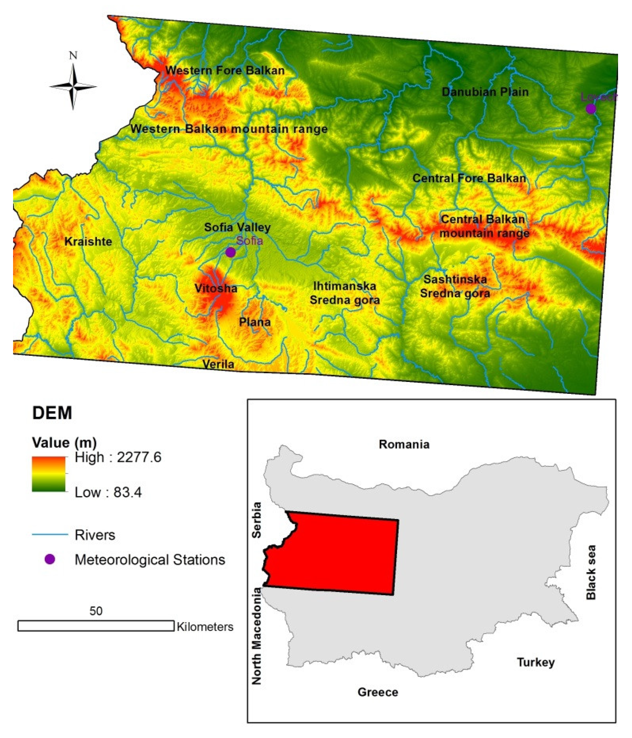
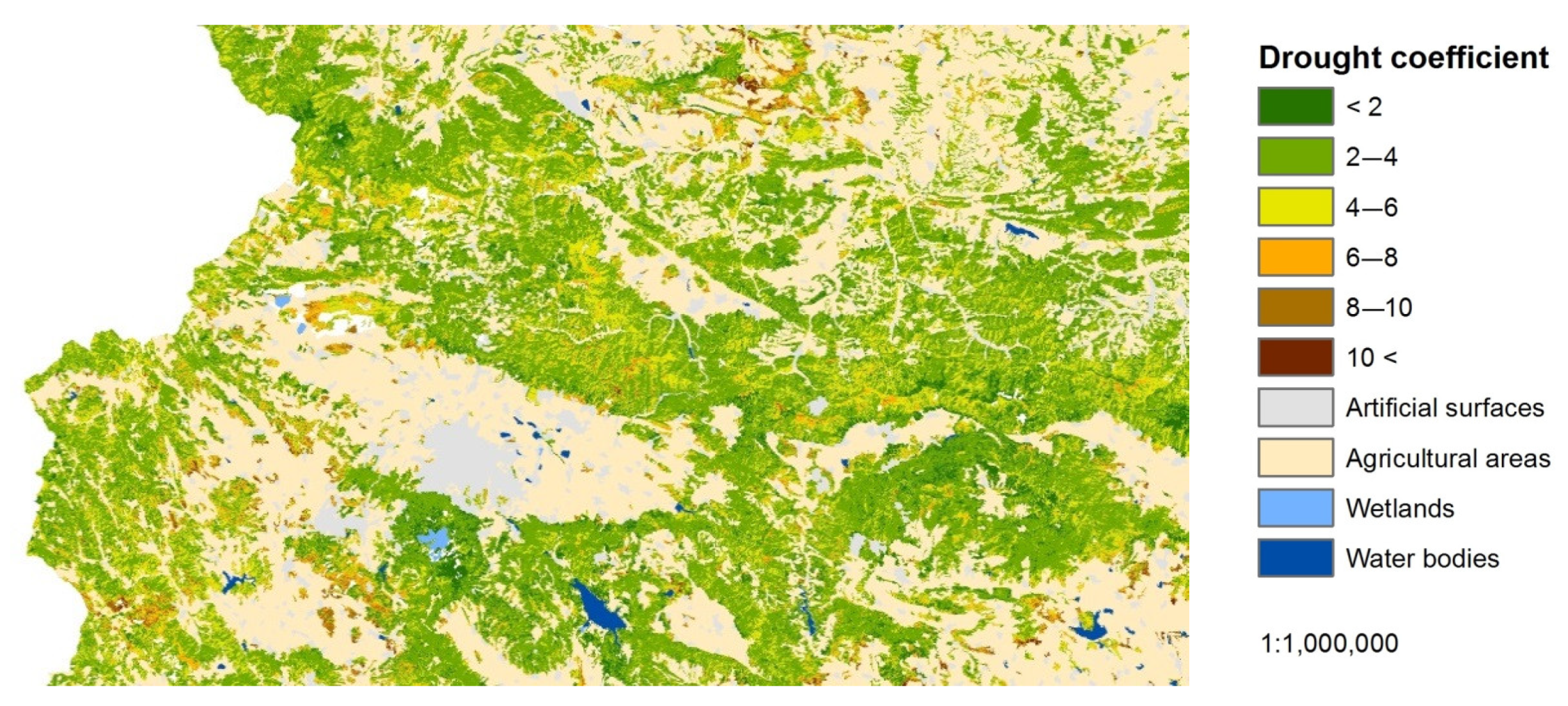
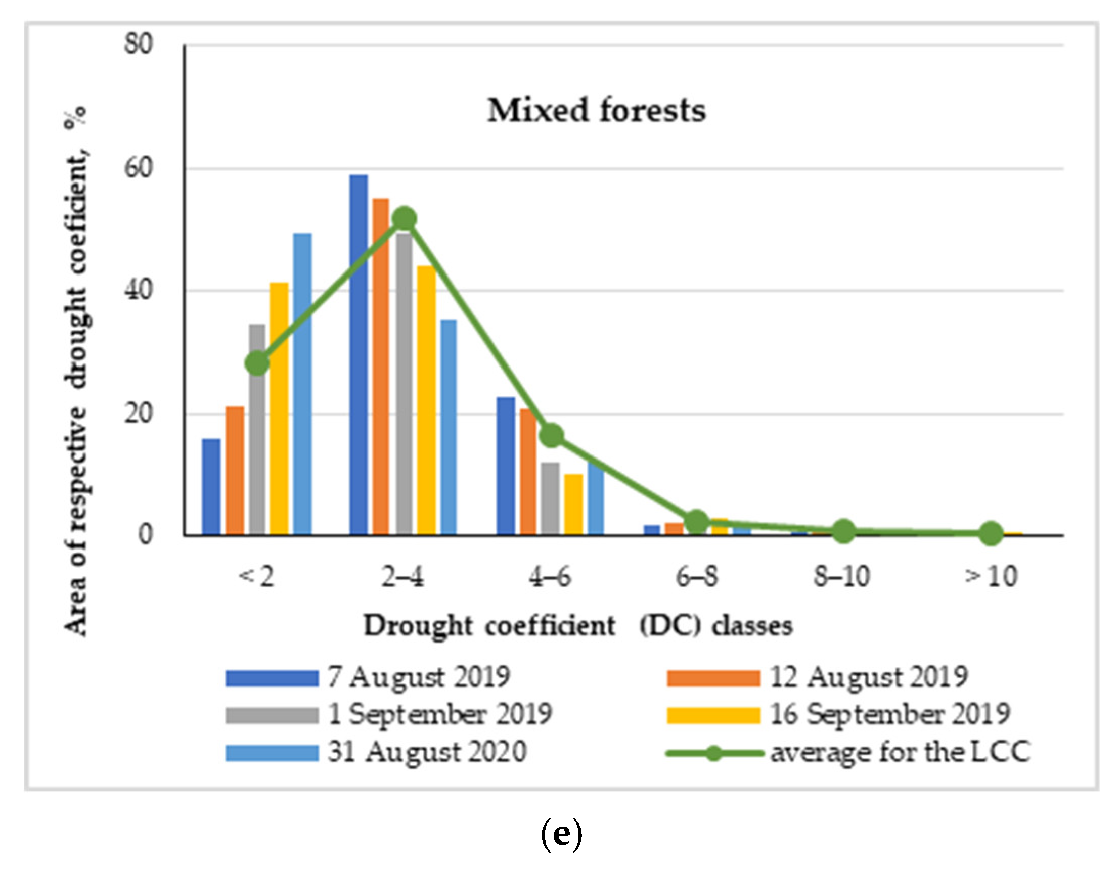
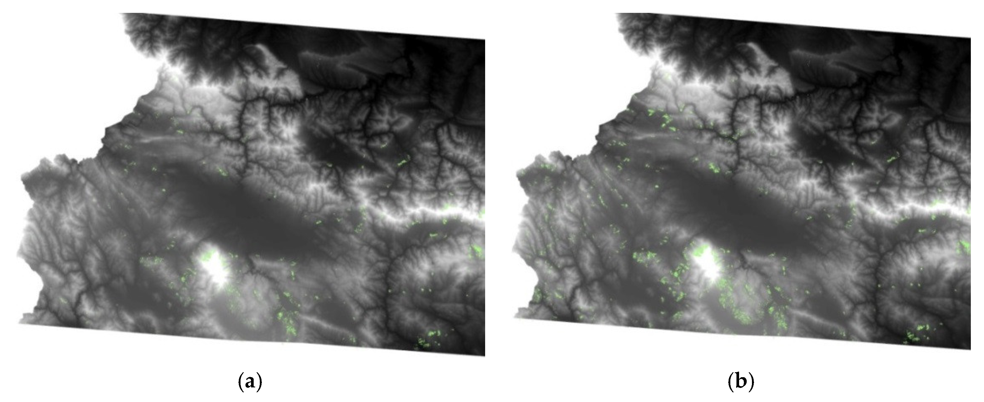
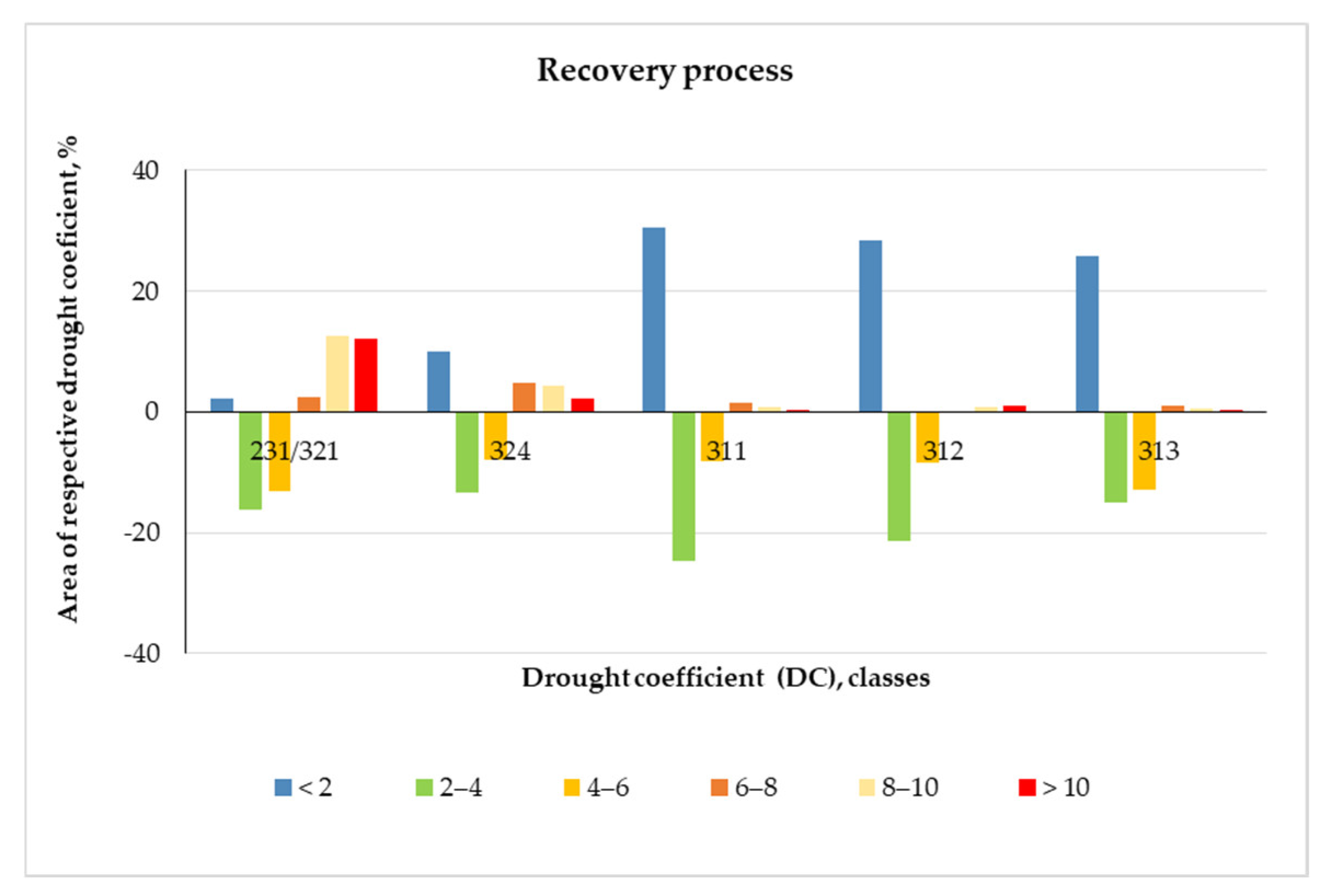
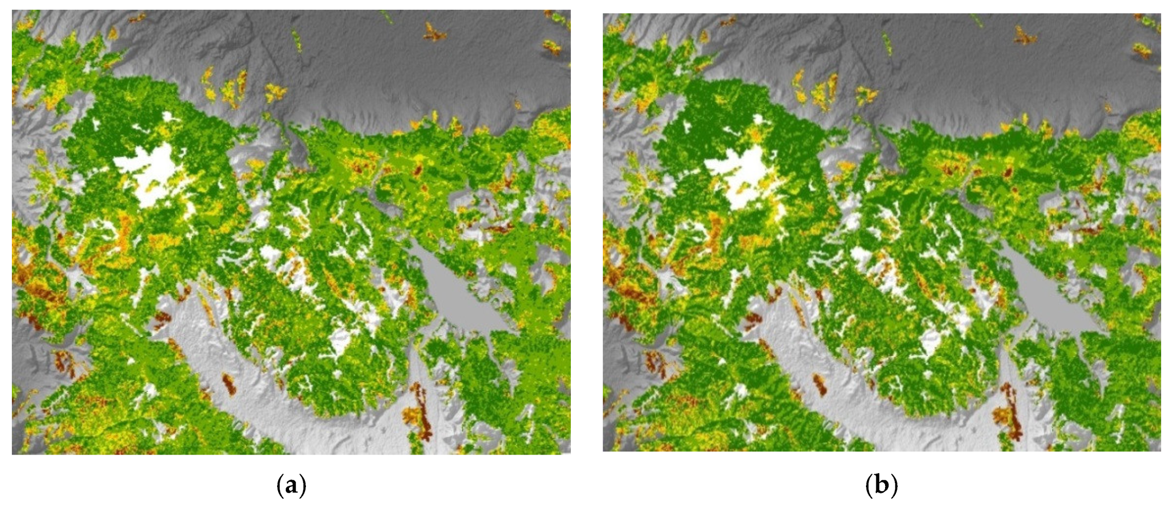
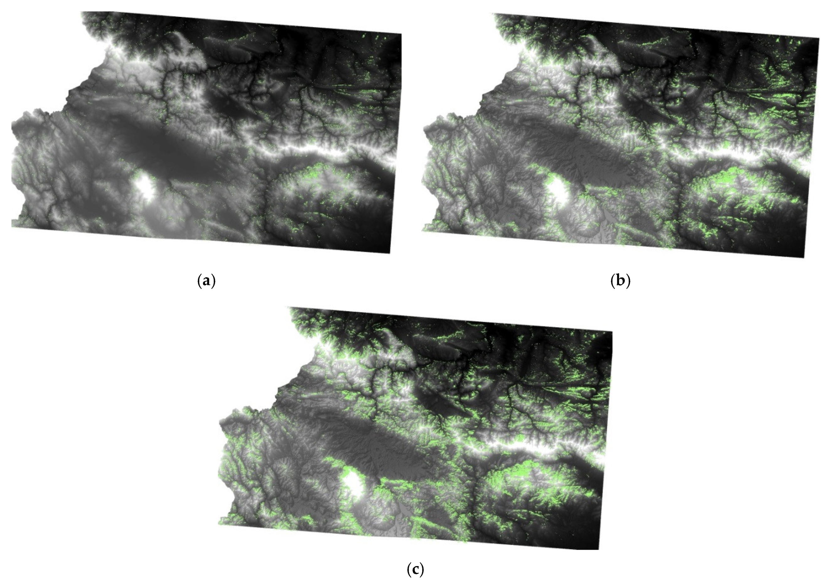
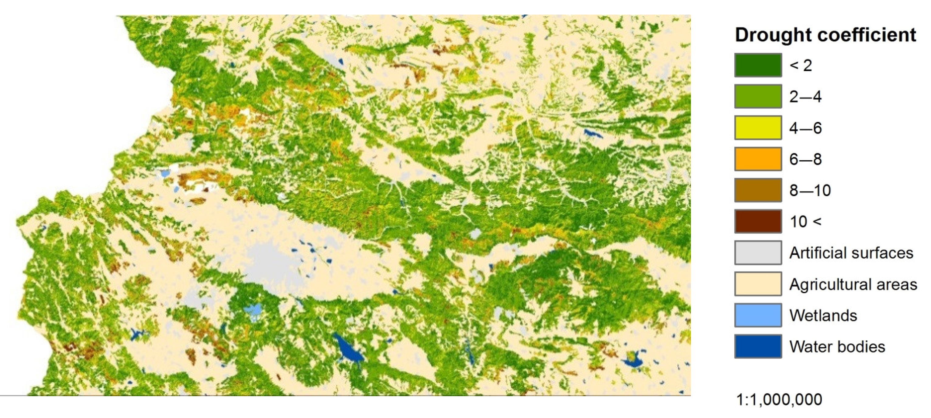
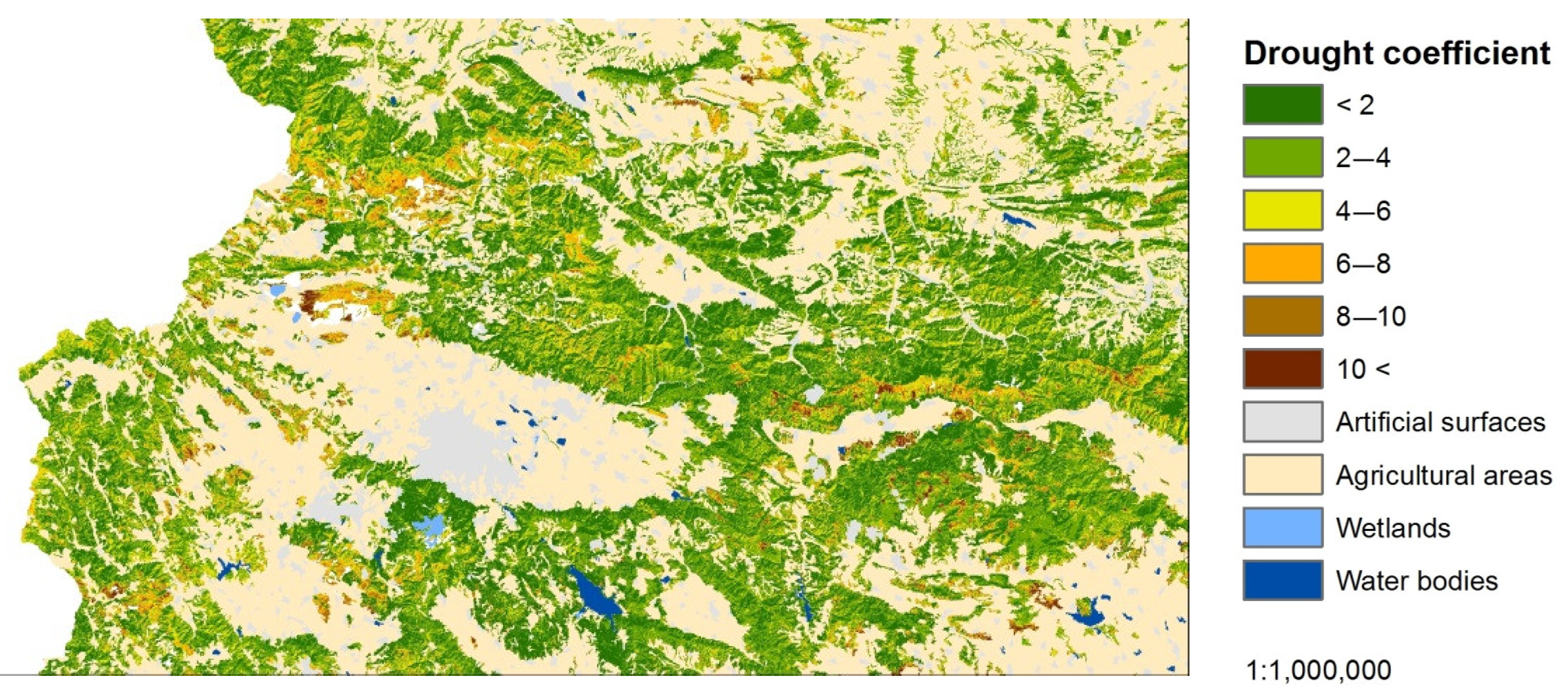
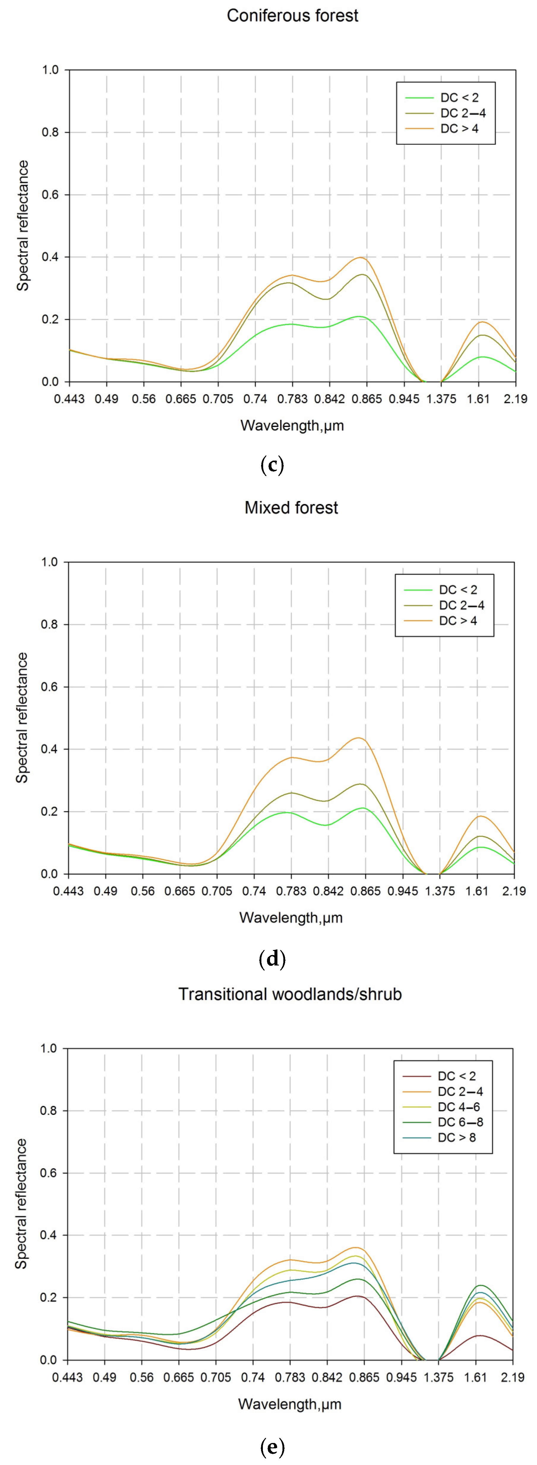
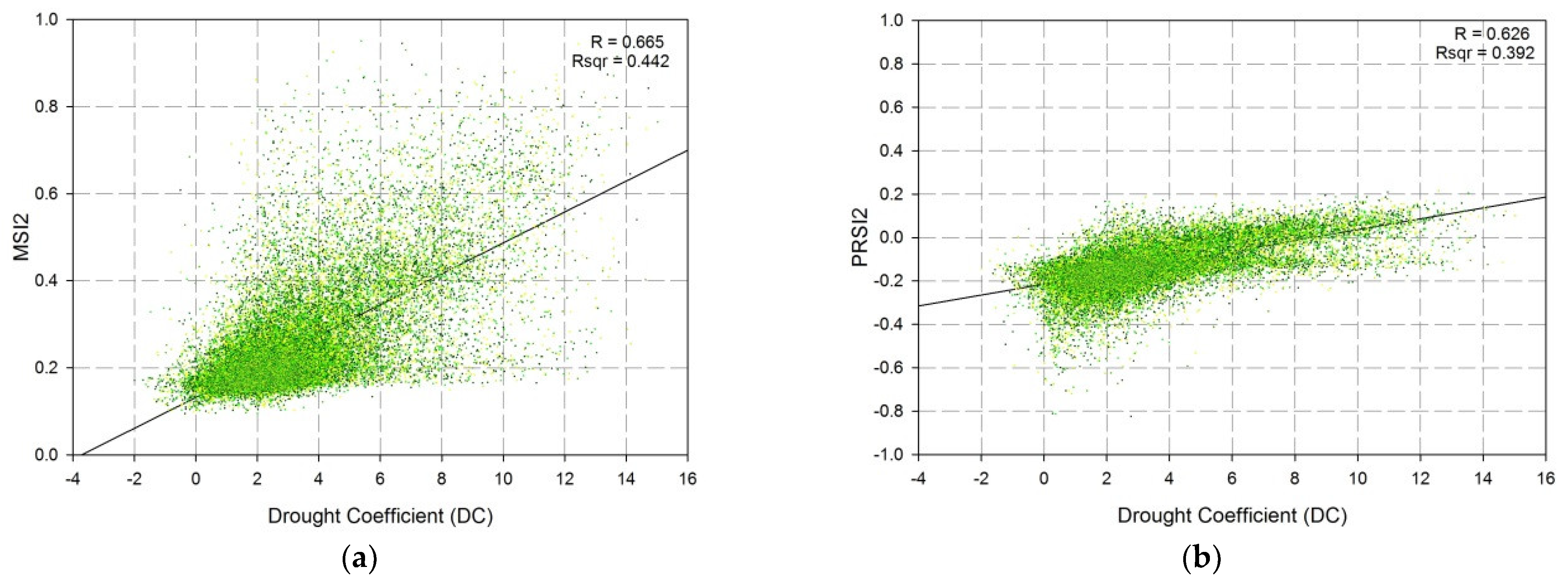
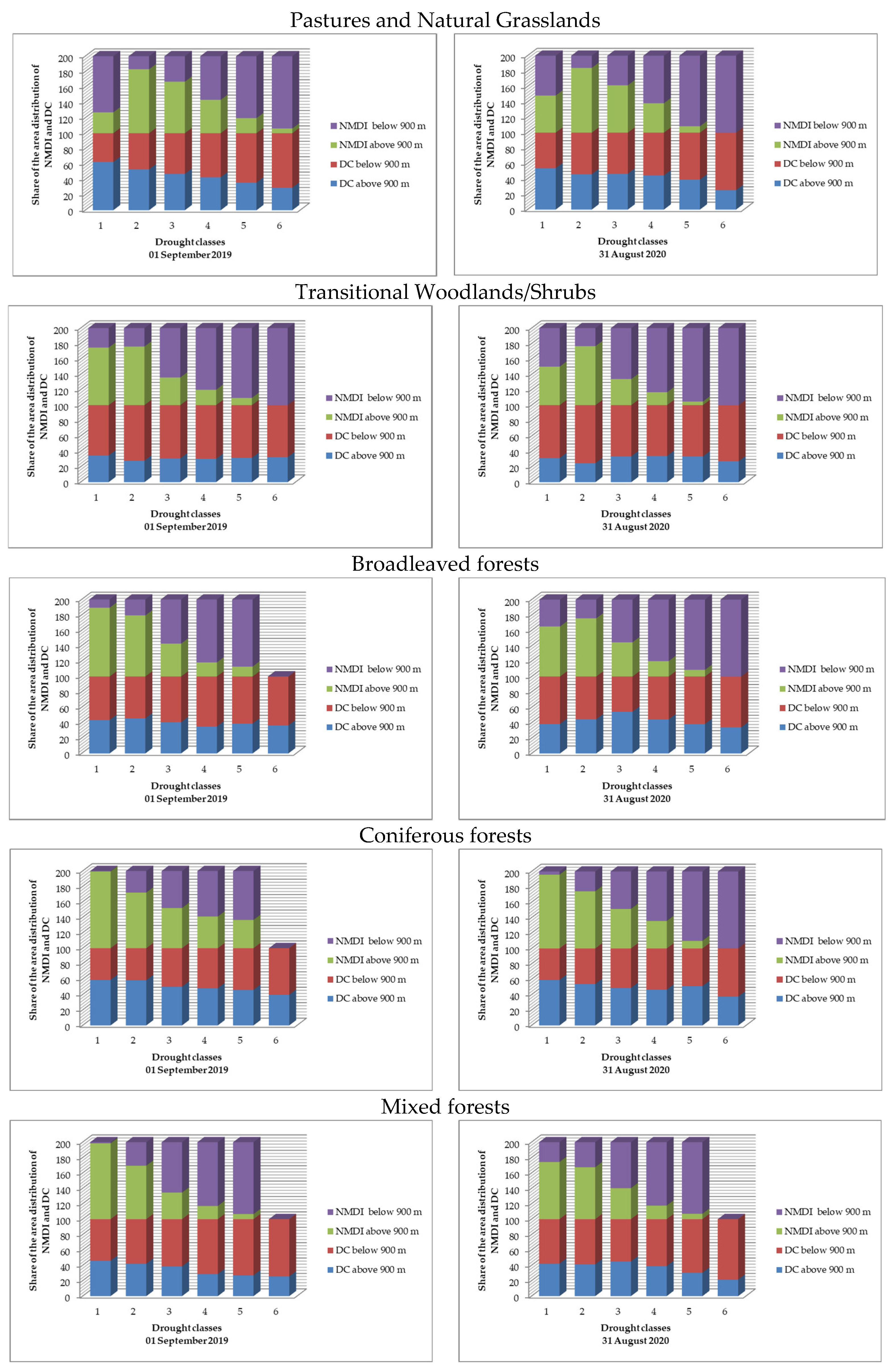
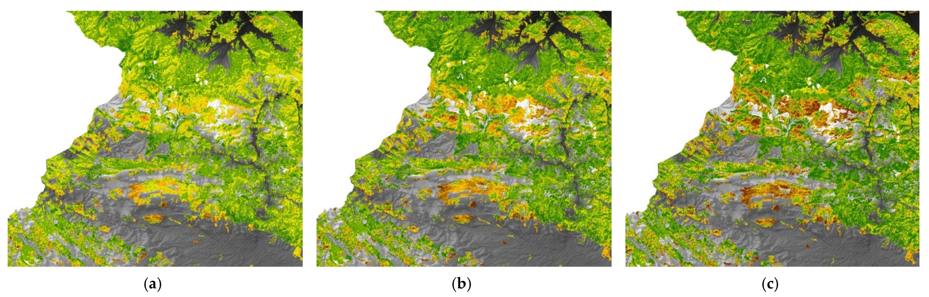
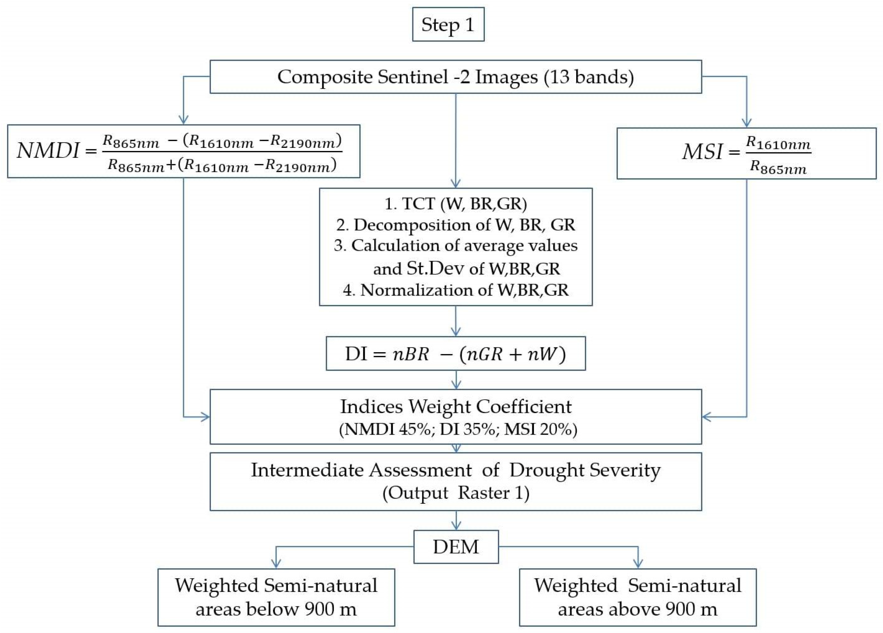
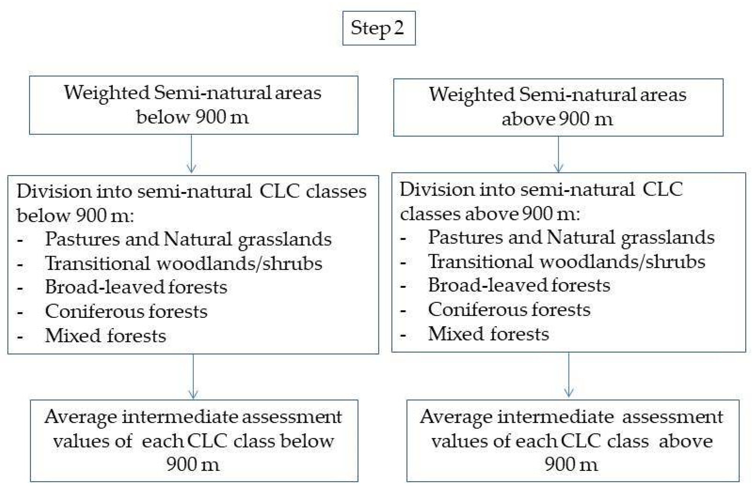
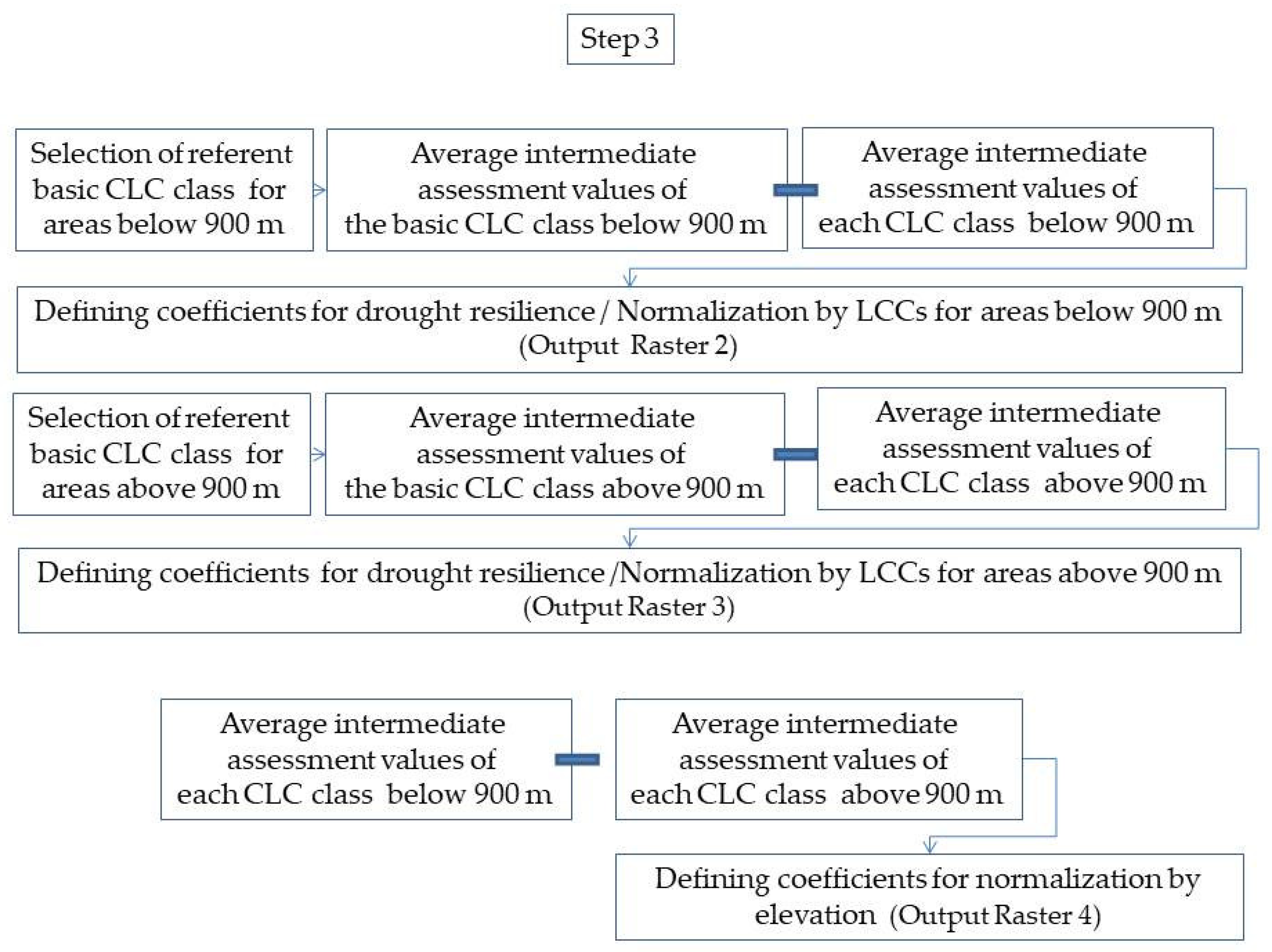
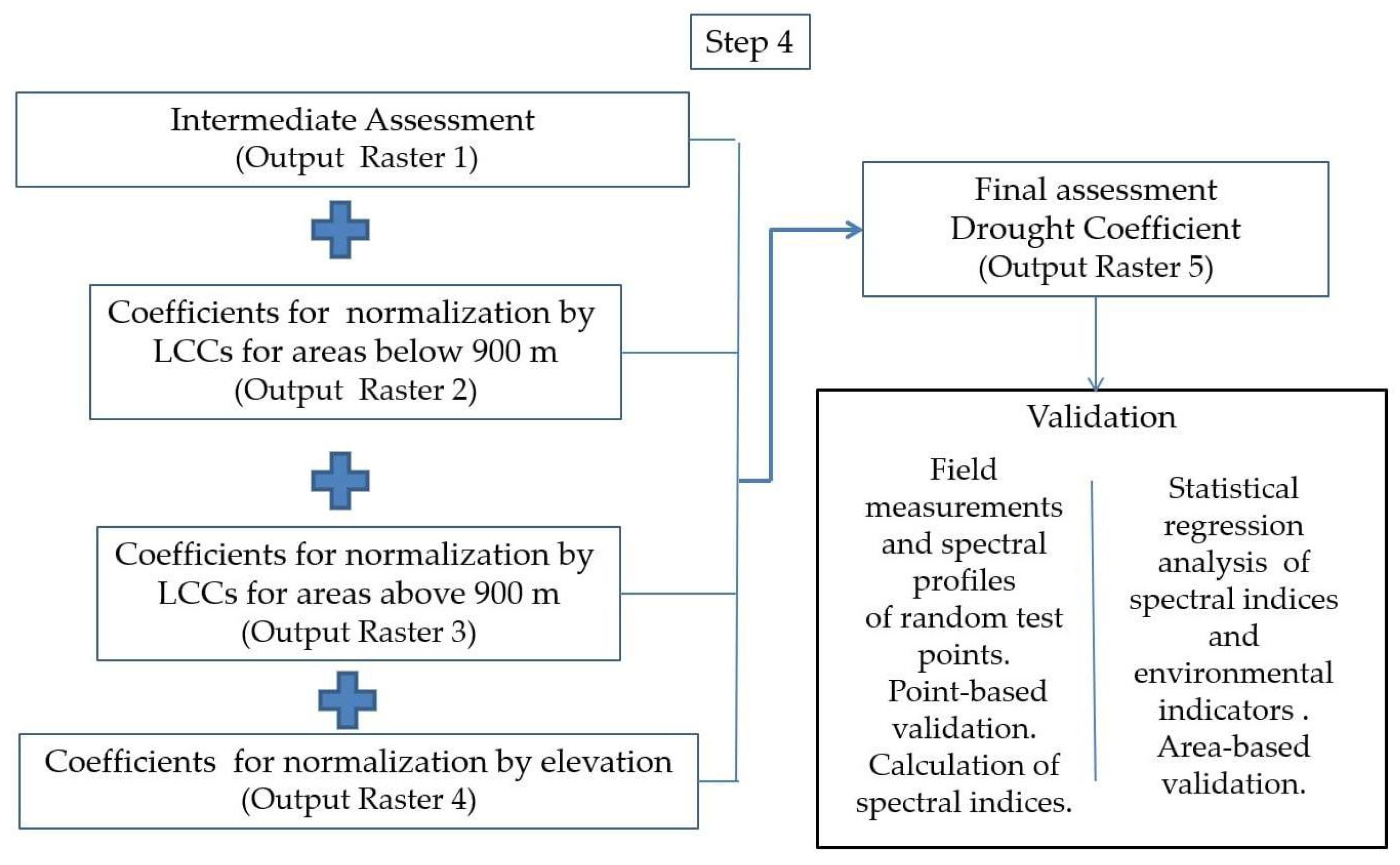
Table 1.
CCC of selected climatic elements between the periods 1961–1990 and 1989–2018.
| Climatic Element | Change in Lovech (%) | CCC Lovech | Change in Sofia (%) | CCC Sofia |
|---|---|---|---|---|
| Annual mean maximum air temperature | 8.4 | 10 | 7.9 | 9 |
| Annual mean minimum air temperature | 16.4 | 5 | 17.6 | 5 |
| Number of ice days | −15.9 | 5 | −13.6 | 5 |
| Number of tropical nights | 200 | 4 | 220 | 5 |
| Mean number of days per year with snow cover | −6 | 1 | 11 | 2 |
| Mean number of days per year with precipitation above 1 mm | 3 | 1 | −3.3 | 1 |
| Average change | 4.3 | 4.5 |
Note: According to Matev (2020) [28].
Table 2.
Acquisition dates of Sentinel-2 satellite images and characteristics of spectral bands used in the study [31].
Table 2.
Acquisition dates of Sentinel-2 satellite images and characteristics of spectral bands used in the study [31].
| Acquisition Dates | Band | Spectral Region | Central Wavelength (μm) | Ground Sampling Distance (m) |
|---|---|---|---|---|
| 7 August 2019 | B1 | 0.443 | 60 | |
| 12 August 2019 | B2 | Blue | 0.49 | 10 |
| 31 August 2020 | B3 | Green peak | 0.56 | 10 |
| B4 | Red | 0.665 | 10 | |
| 1 September 2019 | B5 | Red edge | 0.705 | 20 |
| 16 September 2019 | B6 | Red edge | 0.74 | 20 |
| B7 | Red edge | 0.783 | 20 | |
| B8 | NIR | 0.842 | 10 | |
| B8A | NIR narrow | 0.865 | 20 | |
| B9 | 0.945 | 60 | ||
| B10 | 1.375 | 60 | ||
| B11 | SWIR | 1.61 | 20 | |
| B12 | SWIR | 2.19 | 20 |
Table 3.
Characteristics of the variables used in the final step of the validation process.
| Variable | Sensor | Data of Acquisition | Spatial Resolution |
|---|---|---|---|
| DC | Sentinel-2 | 1 September 2019 | 100 m |
| PSRI2 | Sentinel-2 | 1 September 2019 | 10 m |
| NMDI | Sentinel-2 | 1 September 2019 | 10 m |
| MSI2 | Sentinel-2 | 1 September 2019 | 10 m |
| NMDI | Landsat-8 (OLI) | 28 August 2019 | 30 m |
| MSI2 | Landsat-8 (OLI) | 28 August 2019 | 30 m |
| GDMP | PROBA-V | 31 August 2019 | 300 m |
| FCover | PROBA-V | 31 August 2019 | 1 km |
| LAI | PROBA-V | 31 August 2019 | 1 km |
Table 4.
Distribution of the drought coefficient (DC) classes within the land cover classes (LCCs) in the studied area.
Table 4.
Distribution of the drought coefficient (DC) classes within the land cover classes (LCCs) in the studied area.
| DC Classes | LCCs in % of Studied Area | Average Area for the Representative DC Class for the Studied Period in 2019, in % | ||||
|---|---|---|---|---|---|---|
| 231/321 * | 324 * | 311 * | 312 * | 313 * | ||
| LCCs in % of studied area | 16.8 | 16.6 | 48.0 | 4.8 | 13.8 | |
| <2 | 1.4 | 1.4 | 4.1 | 0.4 | 1.2 | 8.5 |
| 2–4 | 4.1 | 4.0 | 11.7 | 1.2 | 3.4 | 24.3 |
| 4–6 | 4.1 | 4.0 | 11.7 | 1.2 | 3.4 | 24.3 |
| 6–8 | 3.3 | 3.3 | 9.5 | 1.0 | 2.7 | 19.9 |
| 8–10 | 2.6 | 2.6 | 7.4 | 0.7 | 2.1 | 15.5 |
| >10 | 1.3 | 1.3 | 3.6 | 0.4 | 1.0 | 7.6 |
* 231/321—pastures and grasslands; 324—transitional woodlands and shrubs; 311—broadleaved forests; 312—coniferous forests; 313—mixed forests.
Table 5.
Change in the area of the respective Drought coefficient (DC) by periods—in %.
| DC | From the Early August to the Mid-August | From the Mid-August to the Early September | From the Early September to the Mid-September |
|---|---|---|---|
| Pastures and Natural Grasslands | |||
| <2 | 0.5 | 1.9 | −0.1 |
| 2–4 | −4.6 | −8.8 | −2.9 |
| 4–6 | −1.8 | −8.4 | −2.9 |
| 6–8 | 1.1 | 3.0 | −1.6 |
| 8–10 | 2.8 | 7.2 | 2.7 |
| >10 | 1.9 | 5.2 | 4.9 |
| Transitional Woodlands/Shrubs | |||
| <2 | 2.4 | 5.1 | 2.5 |
| 2–4 | −5.9 | −4.2 | −3.3 |
| 4–6 | 0.4 | −6.7 | −1.7 |
| 6–8 | 1.6 | 2.4 | 0.9 |
| 8–10 | 1.0 | 2.4 | 0.9 |
| >10 | 0.4 | 1.0 | 0.9 |
| Broadleaved forests | |||
| <2 | 2.2 | 16.2 | 12.0 |
| 2–4 | −5.5 | −8.2 | −11.0 |
| 4–6 | 2.6 | −9.2 | −1.6 |
| 6–8 | 0.5 | 0.7 | 0.3 |
| 8–10 | 0.1 | 0.4 | 0.2 |
| >10 | 0.0 | 0.2 | 0.1 |
| Coniferous Forests | |||
| <2 | 15.5 | 10.6 | 2.2 |
| 2–4 | −13.0 | −7.0 | −1.4 |
| 4–6 | −3.1 | −4.5 | −1.0 |
| 6–8 | 0.0 | 0.0 | −0.1 |
| 8–10 | 0.3 | 0.5 | 0.0 |
| >10 | 0.2 | 0.5 | 0.2 |
| Mixed Forests | |||
| <2 | 5.4 | 13.5 | 6.9 |
| 2–4 | −3.9 | −5.7 | −5.5 |
| 4–6 | −2.1 | −8.8 | −1.8 |
| 6–8 | 0.3 | 0.4 | 0.3 |
| 8–10 | 0.2 | 0.3 | 0.1 |
| >10 | 0.1 | 0.2 | 0.1 |
Table 6.
Spectral indices values of the individual land cover classes (LCCs) differently affected by drought: pastures and natural grasslands; broadleaved forests; coniferous forests; mixed forests; transitional woodlands/shrubs. The Drought coefficient (DC) classes presents the differently affected by drought point locations (point-based validation).
| Spectral Index | Drought Coefficient (DC) Class | |||||
|---|---|---|---|---|---|---|
| Pastures and Natural Grasslands | ||||||
| <2 | 2–4 | 4–6 | 6–8 | 8–10 | >10 | |
| MSI | 0.54 | 0.72 | 0.73 | 1.41 | 1.51 | 1.68 |
| MSI2 | 0.21 | 0.28 | 0.31 | 0.81 | 0.89 | 0.98 |
| NDVI705 | 0.44 | 0.38 | 0.39 | 0.13 | 0.13 | 0.00 |
| NMDI | 0.57 | 0.48 | 0.47 | 0.44 | 0.40 | 0.35 |
| PSRI | −0.13 | −0.10 | −0.14 | −0.02 | −0.01 | 0.07 |
| PSRI2 | 0.07 | 0.09 | 0.06 | 0.16 | 0.15 | 0.20 |
| Broadleaved Forests | ||||||
| <2 | 2–4 | 4–6 | >6 | n/a | n/a | |
| MSI | 0.40 | 0.54 | 0.50 | 0.51 | n/a | n/a |
| MSI2 | 0.15 | 0.17 | 0.19 | 0.22 | n/a | n/a |
| NDVI705 | 0.56 | 0.53 | 0.55 | 0.50 | n/a | n/a |
| NMDI | 0.62 | 0.55 | 0.57 | 0.54 | n/a | n/a |
| PSRI | −0.15 | −0.16 | −0.13 | −0.10 | n/a | n/a |
| PSRI2 | 0.03 | 0.02 | 0.04 | 0.06 | n/a | n/a |
| Coniferous Forests | ||||||
| <2 | 2–4 | >4 | n/a | n/a | n/a | |
| MSI | 0.44 | 0.55 | 0.58 | n/a | n/a | n/a |
| MSI2 | 0.16 | 0.18 | 0.20 | n/a | n/a | n/a |
| NDVI705 | 0.47 | 0.56 | 0.51 | n/a | n/a | n/a |
| NMDI | 0.63 | 0.59 | 0.55 | n/a | n/a | n/a |
| PSRI | −0.25 | −0.15 | −0.13 | n/a | n/a | n/a |
| PSRI2 | −0.02 | 0.03 | 0.05 | n/a | n/a | n/a |
| Mixed Forests | ||||||
| <2 | 2–4 | >4 | n/a | n/a | n/a | |
| MSI | 0.54 | 0.51 | 0.50 | n/a | n/a | n/a |
| MSI2 | 0.15 | 0.15 | 0.16 | n/a | n/a | n/a |
| NDVI705 | 0.51 | 0.56 | 0.59 | n/a | n/a | n/a |
| NMDI | 0.60 | 0.58 | 0.58 | n/a | n/a | n/a |
| PSRI | −0.23 | −0.21 | −0.12 | n/a | n/a | n/a |
| PSRI2 | 0.00 | −0.01 | 0.03 | n/a | n/a | n/a |
| Transitional Woodlands/Shrubs | ||||||
| <2 | 2–4 | 4–6 | 6–8 | >8 | n/a | |
| MSI | 0.45 | 0.57 | 0.67 | 1.07 | 0.76 | n/a |
| MSI2 | 0.16 | 0.21 | 0.28 | 0.49 | 0.34 | n/a |
| NDVI705 | 0.46 | 0.44 | 0.43 | 0.18 | 0.38 | n/a |
| NMDI | 0.63 | 0.53 | 0.52 | 0.40 | 0.46 | n/a |
| PSRI | −0.26 | −0.08 | −0.13 | −0.06 | −0.13 | n/a |
| PSRI2 | −0.03 | 0.06 | 0.06 | 0.19 | 0.09 | n/a |
Table 7.
Correlation coefficients (in %) between the individual Drought coefficient (DC) classes in the studied semi-natural territories and the spectral indices used in the validation process.
Table 7.
Correlation coefficients (in %) between the individual Drought coefficient (DC) classes in the studied semi-natural territories and the spectral indices used in the validation process.
| Spectral Index | Forest Ecosystems | All Semi-Natural Territories |
|---|---|---|
| MSI | 53.3 | 66.7 |
| MSI2 | 86.7 | 90.5 |
| NMDI | 66.7 | 76.2 |
| NDVI705 | 46.7 | 61.9 |
| PSRI | 60.0 | 61.9 |
| PSRI2 | 86.7 | 71.4 |
Table 8.
Correlation coefficients (in %) between the environmental indicators and the spectral indices used in the area-based validation process.
Table 8.
Correlation coefficients (in %) between the environmental indicators and the spectral indices used in the area-based validation process.
| DC | NMDI-S2 | NMDI-L8 | PSRI2-S2 | MSI2-S2 | MSI2-L8 | |
|---|---|---|---|---|---|---|
| FCover | 27.2 | 41.9 | 37.6 | 42.5 | 45.1 | 42.8 |
| LAI | 28.8 | 45.3 | 40.9 | 46.3 | 44.9 | 39.9 |
| GDMP | 34.4 | 50.5 | 44.1 | 51.8 | 55.9 | 59.2 |
Publisher’s Note: MDPI stays neutral with regard to jurisdictional claims in published maps and institutional affiliations. |
© 2021 by the authors. Licensee MDPI, Basel, Switzerland. This article is an open access article distributed under the terms and conditions of the Creative Commons Attribution (CC BY) license (https://creativecommons.org/licenses/by/4.0/).
Share and Cite
MDPI and ACS Style
Avetisyan, D.; Borisova, D.; Velizarova, E. Integrated Evaluation of Vegetation Drought Stress through Satellite Remote Sensing. Forests 2021, 12, 974. https://0-doi-org.brum.beds.ac.uk/10.3390/f12080974
AMA Style
Avetisyan D, Borisova D, Velizarova E. Integrated Evaluation of Vegetation Drought Stress through Satellite Remote Sensing. Forests. 2021; 12(8):974. https://0-doi-org.brum.beds.ac.uk/10.3390/f12080974
Chicago/Turabian StyleAvetisyan, Daniela, Denitsa Borisova, and Emiliya Velizarova. 2021. "Integrated Evaluation of Vegetation Drought Stress through Satellite Remote Sensing" Forests 12, no. 8: 974. https://0-doi-org.brum.beds.ac.uk/10.3390/f12080974
Note that from the first issue of 2016, this journal uses article numbers instead of page numbers. See further details here.