A Novel Approach to Modelling Stand-Level Growth of an Even-Aged Forest Using a Volume Productivity Index with Application to New Zealand-Grown Coast Redwood

Abstract

Empirical growth models are widely used to predict the growth and yield of plantation tree species, and the precise estimation of site quality is an important component of these models. The most commonly used proxy for site quality in growth models is Site Index (SI), which describes the mean height of dominant trees at a specified base age. Although SI is widely used, considerable research shows significant site-dependent variation in height for a given volume, with this latter variable more closely reflecting actual site productivity. Using a national dataset, this study develops and describes a stand-level growth and yield model for even-aged New Zealand-grown coast redwood (Sequoia sempervirens). We used a novel modelling approach that quantifies site quality using SI and a volume-based index termed the 300 Index, defined as the volume mean annual increment at age 30 years for a reference regime of 300 stems ha⁻¹. The growth model includes a number of interrelated components. Mean top height is modelled from age and SI using a polymorphic Korf function. A modified anamorphic Korf function is used to describe tree quadratic mean diameter (D_q) as a function of age, stand density, SI and a diameter site index. As the D_q model includes stand density in its formulation, it can predict tree growth for different stand densities and thinning regimes. The mortality model is based on a simple attritional equation improved through incorporation of the Reineke stand density index to account for competition-induced mortality. Using these components, the model precisely estimates stand-level volume. The developed model will be of considerable value to growers for yield projection and regime evaluation. By more robustly describing the site effect, the growth model provides researchers with an improved framework for quantifying and understanding the causes of spatial and temporal variation in plantation productivity.

1. Introduction

A central element of forest planning is prediction of plantation growth and yield. Growth models can be broadly grouped as being empirical, process-based or hybrid, although model categorisation is often quite arbitrary as they all lie along a spectrum of empiricism [1]. Empirical models fit statistical relationships to historical growth data and are not explicitly linked to the mechanisms that determine growth [2,3]. Through incorporation of the key physiological processes that influence growth, process-based models can characterise tree and stand development [4,5,6] and are often used for understanding and exploring system behaviour [2,7,8,9]. Hybrid models combine useful features from both statistical and process-based approaches and aim to utilise physiological knowledge while simultaneously incorporating inputs and outputs applicable to forest management [6]. Although these models encompass many variations in structure, they are often more sensitive to the environment than empirical models as they incorporate links to climatic and edaphic information [10,11,12,13] and do not require the parameterisation of process-based models [6]. Although hybrid models and the simpler process-based models are occasionally used by forest managers [14], almost all growth models used for operational management planning are empirical [1].

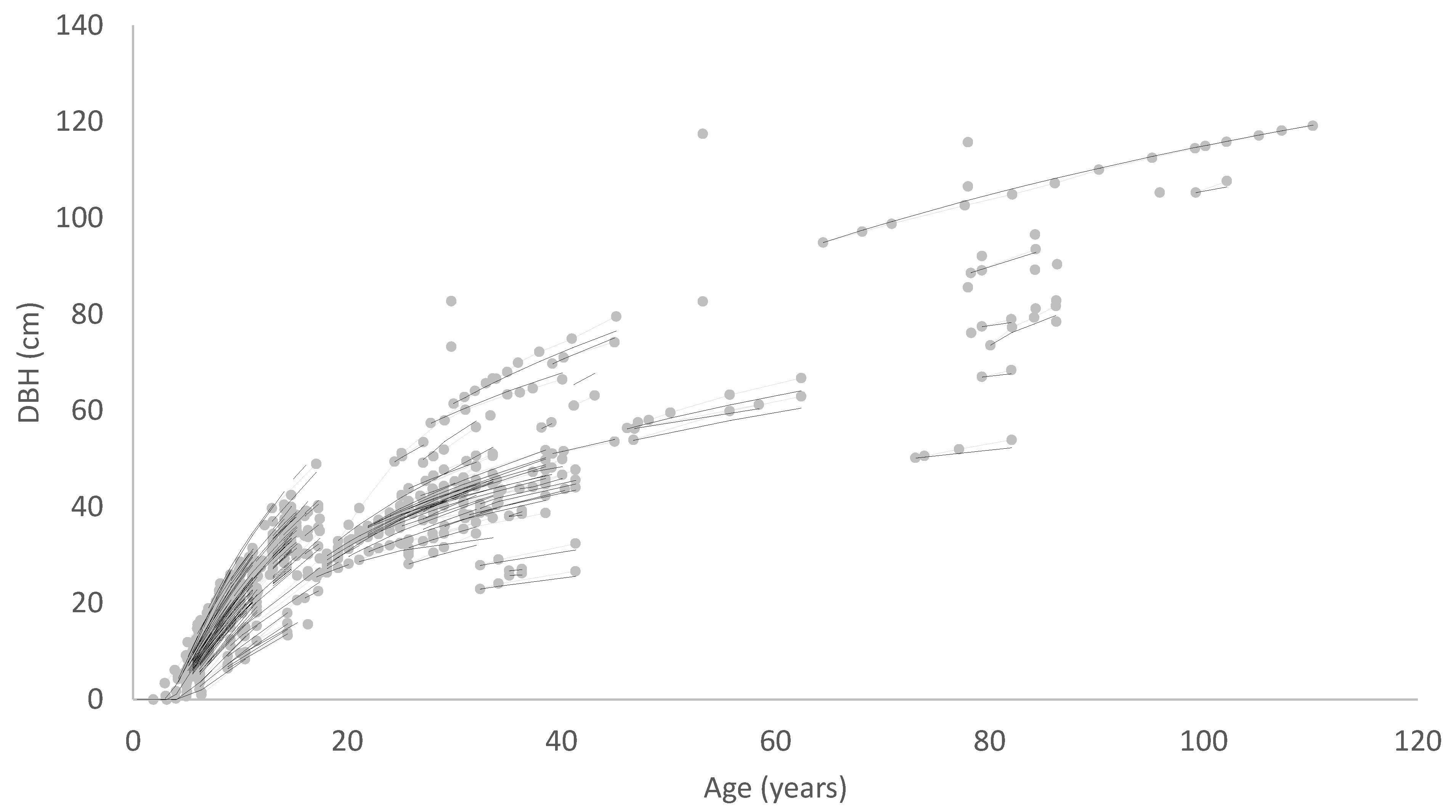
Empirical models may operate at the individual tree level or the stand level as in the model described in this paper. Such models generally include several interlinked components. Growth and mortality functions are a minimum requirement but there are often also functions representing the impacts of silviculture and equations describing relationships between height, diameter and volume. One of the most important elements of a growth and yield model is the inclusion of a robust measure of site quality or productivity [1]. As previously described [15,16], forest site productivity may be assessed in many different ways, including use of geocentric (earth-based) or phytocentric (plant-based) methods. Ideally, proxies for site quality should be correlated with site potential productivity, typically defined for forests as above-ground wood volume [15]. Site quality is most often characterised using Site Index (SI), which is usually defined as the mean height of dominant trees at a specified base age. Site Index was initially justified as a proxy for site quality in the late 19th century [17,18] and then later by Eichhorn’s rule [19] which postulated a strong relationship between height and volume in even-aged stands, regardless of site and stand density.

However, analysis of growth data across a wide range of species has since demonstrated considerable site-dependent variation in volume at a given height [20,21,22,23,24,25,26,27,28], which may vary by as much as 30% [15]. Given the limitations of SI, a metric based on volume is potentially more useful for describing site quality within growth models. However, this is not straightforward because, unlike height, volume is strongly influenced by stand density, especially at young ages. To understand this problem, we first need to consider the process used to incorporate SI into growth model height equations. This involves the following steps described by Bailey and Clutter [29] or more generally using the Generalised Algebraic Difference Approach (GADA) of Cieszewski and Bailey [30]:

(1)

A suitable sigmoidal function for predicting height from age, such as one of those listed by Zeide [31], is chosen.

(2)

One of the model parameters is chosen to act as a site-varying local parameter, transforming the equation into a dynamic model. If this is the asymptote parameter, the model is anamorphic, while if it is the time-scale parameter, the model is polymorphic with a common asymptote.

(3)

The model is reformulated by replacing the local parameter with height at an arbitrary age. This allows it to project height growth from an initial measurement.

(4)

By setting the arbitrary age to the SI base age, the model expresses height as a function of SI and age.

(5)

Finally, the model is inverted to produce an SI equation which predicts SI from height and age.

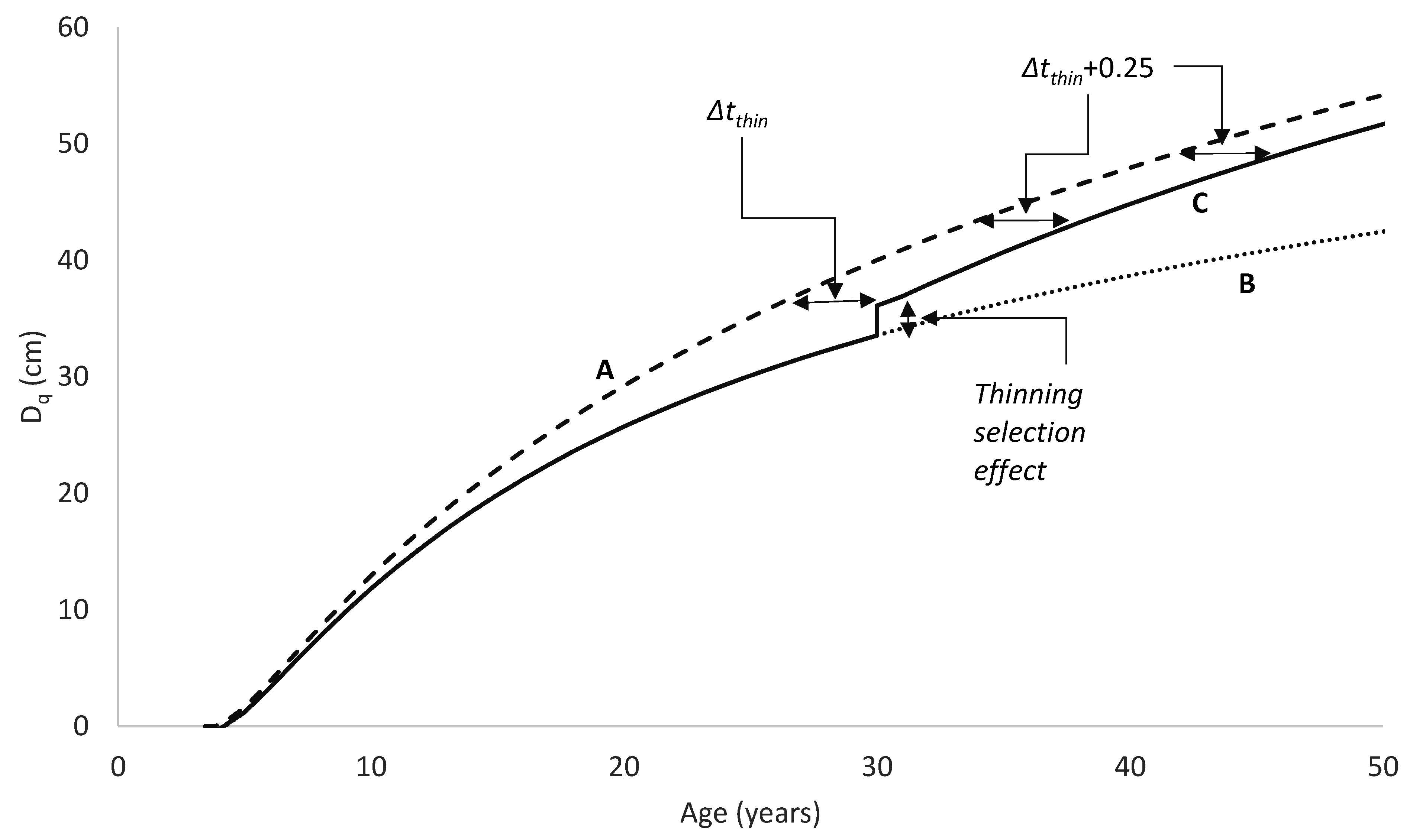
A similar process could be used to develop an equation of diameter growth, although only the first three steps would generally be useful. Steps 4 and 5, which would involve developing an index of diameter at a specified base age, would have little merit because diameter is influenced not only by site but also by stand density. Such a model could be used to project diameter forward in time from an initial measurement but could not readily be used to predict diameter for an alternative stand density at the same site. It would also have limitations in modelling the effects of thinning as it could not distinguish between thinned and unthinned stands with the same diameter and age, which would, however, be expected to follow different growth trajectories. A more fundamental limitation of such a model is that because it accounts for variation in diameter growth rate using a single local parameter, this parameter has to account for the effects of both stand density and site quality on diameter growth. At young ages, before competition develops, diameter is not affected by stand density, but growth rates between stand densities tend to diverge once competition begins to slow the diameter growth of more highly stocked stands. On the other hand, site quality might be expected to produce more of a scaled response, with higher productivity sites providing superior diameter growth at all ages. This suggests that diameter models should account separately for site productivity and stand density.

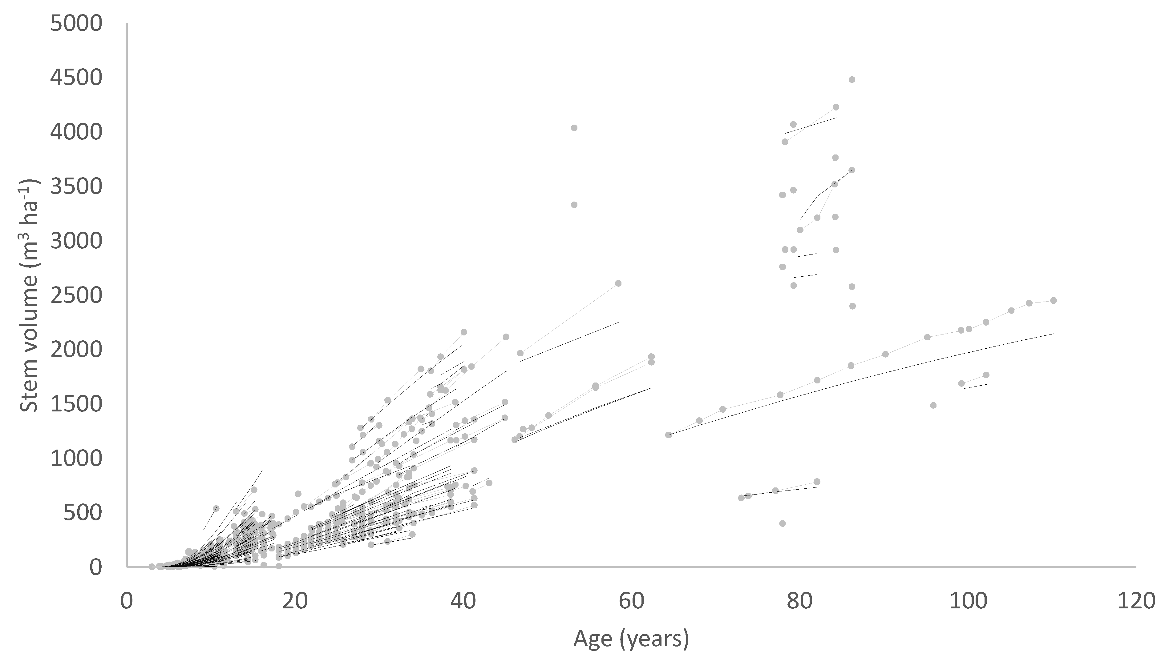
A solution to these problems is to include stand density in the diameter model formulation so that the model predicts diameter as a function of age and stand density. A diameter site index could then be developed, defining diameter at a base age and base stand density. A volume index based on the diameter index and SI which is an index of height productivity could also be derived from such a model. The data requirements for developing a model of this type are somewhat more demanding, consisting, at a minimum, of growth measurements covering a range of stand densities, ages and levels of site productivity. Ideally, measurements from permanent growth plots installed across the population should be supplemented by measurements from trials comprising a range of stand densities at one site.

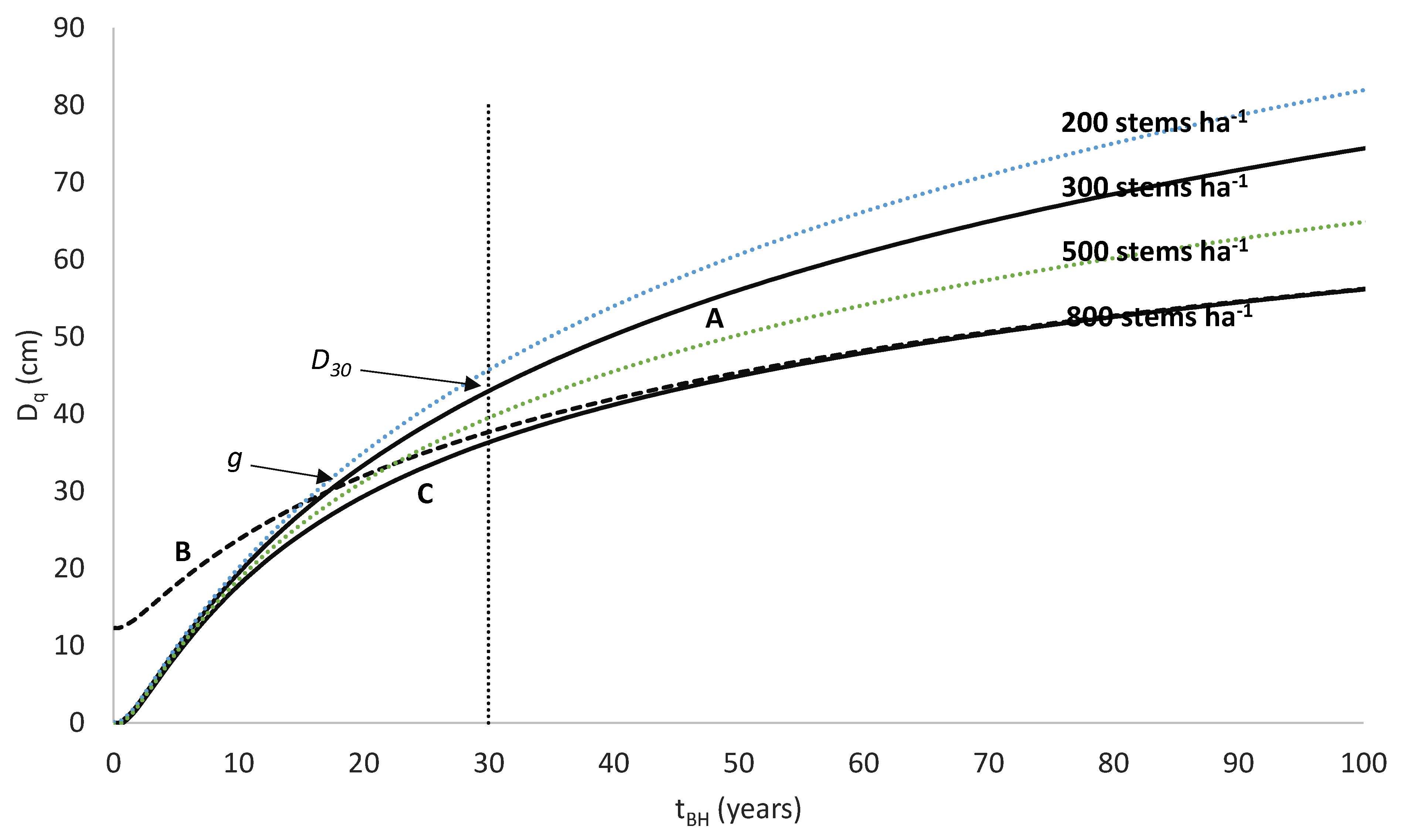
An example of this type of model is the national growth model developed for New Zealand-grown radiata pine (Pinus radiata D. Don), which uses a volume productivity index, the 300 Index [24]. The 300 Index is defined as the stem volume mean annual increment (MAI) at age 30 years for a reference regime with a final stand density of 300 stems ha⁻¹. Research using New Zealand radiata pine plantations has shown that accurate and unbiased values for the 300 Index can be obtained using measurements taken from stands differing in age or stand density from those of the 300 Index reference regime [24]. However, although this growth model has been widely accepted and used for prediction of radiata pine growth and yield within New Zealand, little research has developed similar growth models for other productive plantation species.

Coast redwood (Sequoia sempervirens (Lamb.ex D. Don) Endl.) is a rapidly growing, shade-tolerant, evergreen conifer that is endemic to a narrow coastal strip in central California and southwest Oregon. Individuals within this species include some of the oldest and tallest living trees on Earth, which have reached ages that exceed 2200 years [32,33,34] and heights of 115 m [35]. Outside its native range, redwood has been widely planted within New Zealand, where growth rates of redwood often exceed those of radiata pine on warm sites with little seasonal water deficit [36]. Despite this, radiata pine has been far more widely planted within New Zealand, where it constitutes 90% of plantation area [37], with redwood comprising less than 1% [38]. Given that redwood is one of the most promising alternatives to radiata pine, it would be advantageous to develop a growth model based on the 300 Index so that direct growth comparisons can be made between the two species. Such a growth model would allow growers to optimise site selection and silvicultural treatments for redwood, potentially incentivising further afforestation using this species.

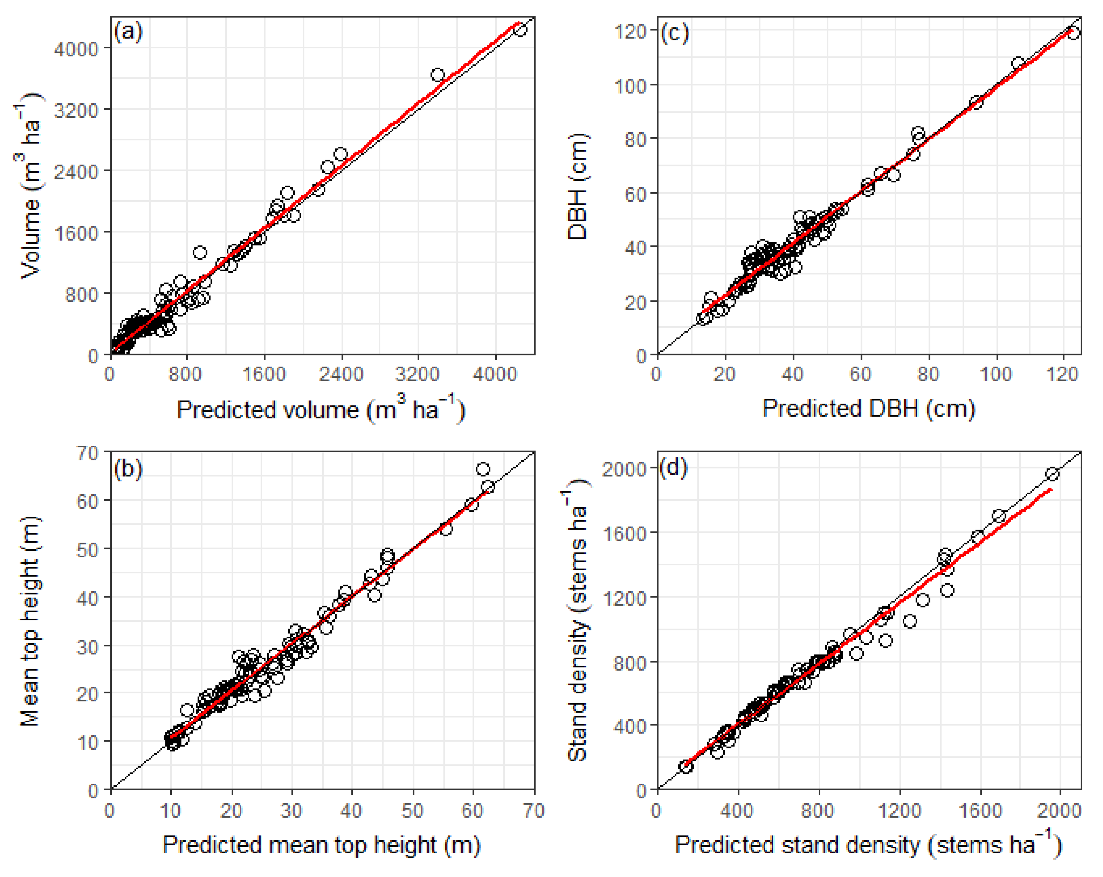
The objective of this study was to develop a stand-level growth model for plantation-grown redwood in New Zealand using two site productivity indices to characterise site quality, namely the 300 Index and SI. Requirements of the model were that it should predict common stand-level forest variables, including mean top height, quadratic mean diameter, stand density, basal area and stem volume, across a variety of stand densities and thinning regimes. This paper presents the structure and fit of the model and provides a comparison of growth predictions for redwood with those produced by an existing radiata pine growth model of similar form.

2. Materials and Methods

2.1. Data

The data used to develop the redwood growth model described in this paper consisted of 743 measurements from 179 permanent sample plots at 62 sites. Plots were considered to be from the same site when they were in close proximity (mostly with a spread of less than one kilometre), with planting year differing by one year at most. There were 24 sites with a single growth plot while a further 24 sites contained multiple plots with a similar stand density. Another 14 sites contained plots with a range of stand densities. In most cases, these sites consisted of single replications of two to four stand densities, but there were also four trials containing two replications of three or four stand densities, and one large stand density and pruning trial with 21 plots.

In each plot, the plot area and measurement age were recorded, with diameter at 1.4-meter breast height (DBH, cm) being measured for all stems and stem height for a sample of trees. Plot area averaged 0.055 ha and ranged from 0.025 to 0.4 ha. The sites were reasonably well distributed throughout New Zealand and covered the range over which redwood is grown [39] as reflected by the wide range in derived (see later methods) SI defined as mean top height at age 30 years (15.0–48.1 m) and 300 Index (2.7–64.7 m³ ha⁻¹ yr⁻¹). The plot data covered a wide range of ages and stand dimensions (

Table 1. Summary of data from 743 measurements in 179 permanent sample plots used to fit the redwood growth model.

Variable	Mean	Std. Dev.	Range
Age (years)	20.9	19.7	0.4–110.2
Mean top height (m)	18.7	12.6	1.7–66.4
Basal area (m2 ha−1)	57.5	59.1	0.0–379.1
Stem volume (m3 ha−1)	445	694	0–4479
Quadratic mean BH diameter (cm)	32.4	22.0	0.2–119.1
Stand density (stems ha−1)	671	300	128–1964

). Stand age ranged from 0.4 to 110 years, while stem volume and height averaged, respectively, 445 m³ ha⁻¹ and 18.7 m, reaching values as high as 4479 m³ ha⁻¹ and 66.4 m (Table 1).

2.2. Analysis Methods

The growth model developed in this study consists of several component sub-models, each predicting a different stand-level variable. These models and the methods of developing them are described in the following subsections.

Firstly, Section 2.2.1 describes how stand metrics used for developing the models were calculated for each plot measurement. Section 2.2.2 describes the mean top height (MTH) sub-model which predicts MTH as a function of stand age, using SI to characterise site quality. Section 2.2.3 presents the DBH/age model which predicts D_q as a function of age and stand density. This model uses both SI and an index of diameter productivity, D₃₀, to account for differences in diameter growth between sites. Section 2.2.4 describes how this D_q model is modified to incorporate thinning effects. A mortality model which predicts stand density as a function of age and D_q is described in Section 2.2.5. The final sub-model is a stand-level volume function, described in Section 2.2.6. This predicts V from BA and MTH, noting that BA can be calculated directly from D_q and N, which are predicted using the two previous sub-models. Section 2.2.7 describes a model for predicting MTH from mean height which, although not part of the growth model, was used when preparing the data.

Although the diameter index D₃₀ is used in the formulation of the DBH/age model, the volume-based 300 Index provides a more useful index of site productivity. As explained in Section 2.2.8, the 300 Index can be calculated directly from SI and D₃₀ using the volume function, and similarly, D₃₀ can be calculated from the 300 Index and SI. This means that D₃₀ can be substituted by the 300 Index when using the model. The sub-models thus predict all relevant stand-level variables at any age based on an initial stand density and thinning history, using the two productivity indices SI and 300 Index to characterise site productivity. However, although estimates of the 300 Index and SI may be known in some cases, more commonly, information on site productivity will be available in the form of plot measurement data. In this case, to apply the model, it is necessary to estimate the 300 Index and SI from the measurement data. The procedures for doing this are briefly described in Section 2.2.8. Finally, Section 2.2.9 describes the methods used to test the model.

2.2.1. Calculation of Stand Metrics

The following stand metrics were obtained for each plot measurement: stand density (N, stems ha⁻¹), mean height (H_mean, m), mean top height (MTH, m), basal area (BA, m² ha⁻¹), quadratic mean DBH (D_q, cm) and total under-bark stem volume (V, m³ ha⁻¹). Mean height and MTH were obtained for each plot measurement by fitting a Petterson Type 1 height/DBH equation to the sample of stems measured for height in the plot and using this equation to predict heights for unmeasured trees. Mean height was calculated as the mean of all stem heights in the plot, measured if available or predicted if not. MTH was defined as the height predicted from the Petterson curve at the mean top diameter, defined as the quadratic mean DBH of the 100 largest diameter stems per hectare (Burkhart and Tennent, 1977). Stem volume was calculated by applying an existing volume and taper function (T458, developed for New Zealand redwood using sectional measurements from several stands) to DBH and measured or predicted height of each stem. All calculations were performed using R [39].

2.2.2. MTH/Age Model

Three forms of sigmoidal growth function were tested for modelling MTH as a function of stand age (t, years), namely the Richards model [40], also known as the Chapman–Richards or Bertalanffy–Richards model; the Weibull model (the integral form of a widely used probability function) and the Korf model [41]. Both anamorphic and common asymptote forms of each model were tested. In addition, for the Korf model, a polymorphic form derived by Cieszewski and Bailey [30] using the GADA method, with properties intermediate between the anamorphic and common asymptote forms, was tested (for convenience, we henceforth refer to this as the ‘polymorphic Korf model’).

Table 2. Model forms tested for predicting a stand-level variable, y, as a function of stand age, t. Each model includes global model parameters c and a or b and an initial value of y, y₀, at age t₀.

Base Model	Form	Equation
Richards	Base form	$y=a{\left(1-e^{-bt}\right)}^c$
	Anamorphic	$y=y_0{\left(\frac{1-e^{-bt}}{1-e^{-b{t}_0}}\right)}^c$
	Common asymptote	$y=a{\left(1-{\left(1-{\left(\frac{y_0}{a}\right)}^{1/c}\right)}^{t/t_0}\right)}^c$
Weibull	Base form	$y=a\left(1-e^{-b{t}^c}\right)$
	Anamorphic	$y=y_0\frac{1-e^{-b{t}^c}}{1-e^{-b{t}_0^c}}$
	Common asymptote	$y=a\left(1-{\left(1-\frac{y_0}{a}\right)}^{{\left(t/t_0\right)}^c}\right)$
Korf	Base form	$y=a{e}^{-b{t}^{-c}}$
	Anamorphic	$y=y_0\frac{e^{-b{t}^{-c}}}{e^{-b{t}_0^{-c}}}$
	Common asymptote	$y=a{\left(\frac{y_0}{a}\right)}^{{\left(t/t_0\right)}^{-c}}$
	Polymorphic	$y=e^{R/2-2b/\left(R{t}^c\right)}$ where $R=ln{y}_0+\sqrt{{\left(ln{y}_0\right)}^2+4b/t_0^c}$

shows the equations for these models (details of their derivation are provided in the Supplementary Material).

To model MTH, an intercept of 0.3 m was included in all models, representing the typical height at planting of nursery-raised redwood seedlings. Thus, the dependent variable of all models in Table 2 was y = MTH − 0.3. Each model accommodated local site effects using the parameter y₀ = SI − 0.3, where SI is defined as MTH at base age t₀ = 30 years. All models were fitted as nonlinear mixed models using the R NLME procedure. In each case, y₀ was fitted as a normally distributed random effect, with mean representing the mean of (SI − 0.3) across all plots, using a nested variance structure (plot nested within site). Thus, for example, the polymorphic Korf model was fitted using the following nonlinear mixed model:

$$MT{H}_{ijk}=0.3+exp(R_{ij}/2-2b/(R_{ij}{t}_{ijk}^c))+e_{ijk}$$

(1)

where

$$R_{ij}=ln({\mu }_{SI}-0.3+s_i+p_{ij})+\sqrt{{\left(ln({\mu }_{SI}-0.3+s_i+p_{ij})\right)}^2+4b/{30}^c}$$

Here, MTH_ijk is the mean top height of measurement k, plot i, site j; t_ijk is its age; µ_SI is the overall mean of (SI − 0.3); s_i is a random effect representing the deviation in SI from the overall mean for site i (assumed to be normally, independently and identically distributed (niid)); p_ij is a random effect representing the deviation in SI from the site mean of plot j (assumed niid); e_ijk is a random error term (assumed niid) and b and c are fixed effect model parameters. Fits of the seven models in Table 2 were compared using the Akaike Information Criterion (AIC).

By inverting the equation of the best fitting model, SI was estimated for each plot from the final measurement, as was the age t_1.4 when the plot achieved an MTH of 1.4 m (breast height). Details of these procedures are given later in the paper. Breast height age, t_BH, was calculated using t_BH = t − t_1.4. SI and t_BH were used in subsequent modelling of DBH.

2.2.3. DBH/Age Model

The central component of the redwood growth model is an equation for predicting D_q from stand age. Note that it is more common for stand-level models to predict BA rather than D_q. However, because the redwood D_q model described here includes stand density in its formulation, with the latter being predicted using the mortality function described later in the paper, it is straightforward to estimate BA from the D_q model. To derive the D_q model, the first step was to test the model forms listed in Table 2 for predicting D_q as a function of t_BH = t − t_1.4 (years). Breast height age rather than age since planting was used to ensure that D_q was predicted to be zero at an MTH of 1.4 m. Thus, the dependent variable of all Table 2 models tested in this step was y = D_q, with t_BH as the independent variable. Each model accommodated local site effects using the parameter y₀ = D₃₀, where D₃₀ was defined as D_q at base age t₀ = 30 − t_1.4 years (i.e., 30 years after planting). The models were fitted using the R nonlinear mixed model NLME procedure using a nested variance structure (plot nested within site) similar to the MTH models. The best fitting model was chosen based on the AIC and used in subsequent steps.

The model fitted in Step 1 did not include stand density in its formulation, and the next step was to incorporate this into the model. An approach similar to that employed with the radiata pine 300 Index growth model [24] was used. In brief, the 300 Index model predicts D_q as a function of age, stand density and SI, using a local parameter to describe the site. Details of the development and form of the diameter model are only described in unpublished reports and are therefore briefly outlined here. The 300 Index model form was developed following close examination of growth data from radiata pine stand density trials. This revealed the following six properties:

(1)

DBH growth at a low reference stand density followed a typical sigmoidal growth pattern.

(2)

At young ages, DBH growth was identical for all stand densities.

(3)

Once competition began, DBH growth at higher stand densities slowed compared with the reference stand density.

(4)

At lower productivity sites, competition began at a smaller mean DBH than at higher productivity sites.

(5)

Once competition began, the DBH growth rate at a given stand density was reduced by a constant proportion compared with the reference stand density, and this proportion remained constant over time.

(6)

The proportion reduction was a linear function of the log of stand density.

A function was developed based on these properties and used in the radiata pine 300 Index model. The D_q model developed for redwood is similar and has the following form:

$$D_q=D(t_{BH})-(d/f)(lnN-ln300)ln\left(1+exp(f(D(t_{BH})-g))\right)$$

(2)

where N is stand density (stems ha⁻¹); d, f and g are model parameters; and where D(t_BH) is the predicted D_q for a stand growing at a density of 300 stems ha⁻¹, which is predicted as a function of t_BH using the best fitting sigmoidal model from Step 1.

The behaviour of Equation (2) using parameter estimates obtained from the redwood data as described later in the paper is illustrated in Figure 1. At a reference stand density of 300 stems ha⁻¹, the growth of D_q follows the sigmoidal curve shown by line A, $y=D$(t_BH), satisfying Property 1 above. Growth at a stand density of 800 stems ha⁻¹ shown by line C initially follows line A, satisfying Property 2. However, at older ages, D_q growth slows (Property 3) and converges towards line B, $y=kg+(1-k)D(t_{BH}),$ where $k=d(ln800-ln300)$. Note that the growth rate of line B is reduced by a constant amount compared with the reference line A depending on the stand density, with the extent of the reduction controlled by d. This satisfies Properties 5 and 6. The midpoint of this transition occurs at D_q = g, when the growth rate of D_q is midway between that of lines A and B. The parameter f controls how rapidly the transition from pre-competition to post-competition growth occurs. Note that at stand densities of less than 300 stems ha⁻¹, the model predicts that D_q growth will be greater than at the reference density.

The choice of using 300 stems ha⁻¹ for the reference stand density in Equation (2) was arbitrary, but testing suggests that the model fit is fairly insensitive to the value chosen. Ideally, the reference stand density should be low so that the curve y = D(t_BH) represents competition-free diameter growth. However, the model may be difficult to fit if the chosen value is outside the range of stand densities represented in the data. Therefore, a value of 300 stems ha⁻¹ was considered appropriate and also simplified incorporation of the 300 Index into the model system, as will be described later. Variations of the model were also tested (e.g., we tested using N rather than ln(N)), but Equation (2) was chosen as the best fitting model.

The model represented by Equation (2) was fitted using the R nonlinear mixed model NLME procedure using a nested variance structure (plot nested within site), with local site effects accounted for by the parameter y₀ = D₃₀ which, in this model, represents D_q at age 30 years and 300 stems ha⁻¹. Thus, for example, the anamorphic Korf model was fitted using the following nonlinear mixed model:

$$D_q{}_{ijk}=D\left(t_{BH}{}_{ijk}\right)-(d/f)(lnN-ln300)ln\left(1+exp\left(f\left(D\left(t_{BH}{}_{ijk}\right)-g\right)\right)\right)+e_{ijk}$$

(3)

where

$$D\left(t_{BH}{}_{ijk}\right)=\left({\mu }_{D_{30}}+s_i+p_{ij}\right)exp\left(-b{t}_{BH}{{}_{ijk}}^{-c}\right)/exp(-b{(30-t_{1.4})}^{-c})$$

Here, $D_q{}_{ijk}$ is the quadratic mean DBH of measurement k, plot i, site j; $t_{BH}{}_{ijk}$ is its breast height age; ${\mu }_{D_{30}}$ is the overall mean of D₃₀; s_i is a random effect representing the deviation in D₃₀ from the overall mean for site i (assumed niid); p_ij is a random effect representing the deviation in D₃₀ from the site mean of plot j (assumed niid); e_ijk is a random error term (assumed niid); and b, c, d, f and g are fixed effect model parameters. A likelihood ratio test was used to test the statistical significance of the improvement in fit of this model compared with the best fitting Step 1 model.

Examination of the redwood data indicated that the D_q when competition begins can vary with site, as also noted for radiata pine (Property 4 above). Specifically, competition appears to begin at a smaller D_q in stands with low SI. This effect can be included in Equation (2) or (3) by expressing the parameter g as a linear function of SI:

$$g=g_1+g_2(SI-30)$$

(4)

For convenience, we subtract 30 from SI so that g₁ represents the D_q when competition is initiated for a typical site with SI = 30.

2.2.4. Incorporating Thinning Effects into the DBH Model

The model described in Section 2.2.3 predicts D_q as a function of the site productivity indices D₃₀ and SI, breast height age (t_BH) and stand density (N). However, this model cannot be directly applied to stands following thinning as it would result in a discontinuity in predicted DBH due to the instant change in stand density at thinning. Incorporating a realistic thinning effect into this model was achieved as follows.

Suppose a stand is thinned at breast height age t_thin from N₁ to N₂ stems ha⁻¹. As there is generally a selection effect at thinning with smaller stems being removed, the basal area after thinning, BA₂, will generally form a higher proportion of the basal area prior to thinning, BA₁, than indicated by the simple ratio of stems remaining. As we had inadequate thinning data to quantify this effect for New Zealand redwood stands, we used the following relationship developed from New Zealand radiata pine thinning data:

$$B{A}_2/B{A}_1={(N_2/N_1)}^{0.78}$$

(5)

This led to the following relationship for predicting D_q following thinning, D₂, from its value prior to thinning, D₁:

$$D_2=D_1{(N_1/N_2)}^{0.11}$$

(6)

In a thinned stand, D_q growth prior to thinning is predicted using Equation (2) with the appropriate pre-thinning stand density. This provides D₁. The D_q immediately following thinning, D₂, is then calculated using Equation (6). The age t’ when Equation (2) predicts D_q to equal D₂ is then obtained (this requires an iterative procedure using the bisection method which is described in the Supplementary Material). If the difference Δt_thin = t’ − t_thin is positive, it represents the loss in development time due to carrying a higher stand density prior to thinning compared with a stand grown from planting at the post-thinning stand density. However, in stands thinned at a young age, this may be outweighed by the thinning selection effect, in which case Δt_thin will be negative. Regardless of this, D_q growth of the post-thinning stand is predicted using Equation (2) with t_BH replaced by t_BH − Δt_thin. One further refinement to this procedure used in the radiata pine 300 Index model is to increase Δt_thin by an additional small amount to account for crown expansion following thinning; in the radiata pine model, it is increased by 50%, up to a maximum of 0.25 years. This procedure was adopted in the redwood model as there were no data available to test the effect for redwood. This additional time shift is introduced one year following thinning and is maintained from that point onwards. The procedure is illustrated in Figure 2.

As some of the plots in the measurement data had received thinning prior to their first measurement, it was desirable to adjust for these thinning events when fitting the model. To achieve this, after the parameters of Equation (2) were estimated in Step 2, Δt_thin was calculated for each plot using the above procedure, and the model was refitted using t − t_1.4 − Δt_thin as the independent variable. This process was repeated until parameter estimates converged, which was achieved in five iterations.

2.2.5. Mortality Model

Mortality in forest plantations can be categorised into three types: attritional or low-level mortality not due to catastrophic events or excessively high stand densities; catastrophic mortality occurring as a result of rare extreme events such as storms, fires or droughts; and competition-induced mortality in highly stocked stands. A model of constant attritional mortality is represented by the following equation:

$$N_1=N_0{(1-k)}^{\Delta t}$$

(7)

where N₀ and N₁ are stand densities in stems ha⁻¹ at the beginning and end of a measurement increment represented in the data, respectively; Δt is the length of the increment in years and the parameter k represents the annual attritional mortality rate (possibly including a component from rare catastrophic events). However, this model takes no account of competition-induced mortality.

The well-known stand density index of Reineke (1933) provides a measure of the level of competition in a stand. For metric measurements, this index is calculated as follows:

$$SDI=N{D}_q^{1.6}/437.1$$

(8)

where N (stems ha⁻¹) is the stand density and D_q (cm) is the quadratic mean DBH. It is reasonable to assume that competition-induced mortality will increase with increasing SDI, suggesting the following modification to Equation (7):

$$N_1=N_0{(1-k-m{(SDI/1000)}^n)}^{\Delta t}$$

(9)

where k, m and n are model parameters, with k representing the attritional mortality rate and the other two parameters controlling competition-induced mortality based on SDI (divided by 1000 for convenience). The parameters of Equations (7) and (9) were estimated from the measurement increments using the R bnlr (binomial regression) procedure with logistic link and binomial error function. When implemented, this model is not invariant to step length because SDI changes during the time covered by a model step. As it was intended to implement the model using a one-year step length, the value of SDI used for fitting the model was obtained by calculating SDI at the beginning and end of each measurement increment, and linear interpolation was used to determine its value at age $t+ t/2-1/2$.

2.2.6. Stand-Level Volume Function

The following stand-level volume function based on a radiata pine model [42] was fitted to predict the under-bark stem volume for each plot measurement from MTH and BA using the NLS procedure in R:

$$V_i=vMT{H}_{i}B{A}_i{(MT{H}_i-1.4)}^{-w}+e_i$$

(10)

where V_i (m³ ha⁻¹), MTH_i (m) and BA_i (m² ha⁻¹) are, respectively, stem volume, MTH and BA for plot/measurement i; v and w are model parameters and e_i is a niid error term. The model was fitted to all measurements with MTH greater than 5 m.

2.2.7. Model for Predicting MTH from Mean Height

A nonlinear regression model was fitted to predict MTH from mean height and stand density using the NLS procedure in R:

$$MT{H}_i=H_{mean}{}_i/\left(1+r\left(1-exp(s(N_i-100))\right)\right)+e_i$$

(11)

where MTH_i (m), $H_{mean}{}_i$ (m) and N_i (stems ha⁻¹) are, respectively, MTH, mean height and stand density for plot/measurement i; r and s are model parameters and e_i is a niid error term. This model was used to predict MTH for plot measurements where MTH was not available (e.g., in very young stands where trees were less than 1.4 m tall).

2.2.8. Estimation of the 300 Index from a Plot Measurement

The model can be used to estimate the 300 Index from a plot measurement using the following procedure. Firstly, SI is estimated from MTH and age by inverting the height/age model; details of this are presented later in the paper. Although it is not possible to invert Equation (2) to predict D₃₀, this can be estimated easily using an iterative procedure such as the bisection method from a plot measurement consisting of age, stand density, BA and SI, along with thinning history. Details of a method for doing this are provided in the Supplementary Material. Once SI and D₃₀ are estimated from a plot measurement, the volume function (Equation (10)) can be used to estimate the 300 Index (I₃₀₀) based on its definition (stem volume MAI at age 30 years for a stand density of 300 stems ha⁻¹), as follows:

$$I_{300}=vSI(300\pi D_{30}^2/40\text{,}000){(SI-1.4)}^{-w}/30$$

(12)

$$=0.00025\pi v{D}_{30}^{2}SI{(SI-1.4)}^{-w}$$

By inverting this equation, D₃₀ can be calculated from I₃₀₀ and SI, allowing the model to be applied to a stand of known SI and 300 Index:

$$D_{30}=200\sqrt{30I_{300}/(300\pi vSI{(SI-1.4)}^{-w})}$$

(13)

Using these procedures, SI, D₃₀ and the 300 Index were calculated for each plot in the measurement database. The index BA₃₀, representing BA at 300 stems ha⁻¹ and age 30 years, was also estimated using the following:

$$B{A}_{30}=0.0075\pi D_{30}^2$$

(14)

Distributional statistics for each variable were calculated and correlations between them determined.

2.2.9. Model Testing

A test version of the complete growth model incorporating all the above equations was implemented as an Excel VBA application and used to test the performance of the model (this spreadsheet is provided in the Supplementary Material). As growth data for redwood in New Zealand are limited, it was considered necessary to use all available data to develop the model, and a formal validation of the model against independent data was therefore not possible. As an initial step, the model performance was tested against the data used to develop it by plotting predicted against actual values and by comparing actual with predicted growth increments across a range of stand and site parameters. It is intended that testing of the model will be ongoing as new measurement data become available.

3. Results

3.1. MTH/Age Model

Based on the AIC, the Korf model performed better than either the Richards or Weibull model for predicting MTH from age (

Table 3. Akaike Information Criterion (AIC) of nonlinear mixed models for predicting MTH from stand age.

Model	Form	AIC
Richards	Anamorphic	2526.2
	Common asymptote	2574.9
Weibull	Anamorphic	2583.6
	Common asymptote	2631.6
Korf	Anamorphic	2412.4
	Common asymptote	2411.5
	Polymorphic	2384.7

). The common asymptote and anamorphic forms of this model fitted almost equally well, suggesting the true behaviour lay somewhere between these two extremes. This was confirmed by the fit of the polymorphic form of the model, which had the lowest AIC of all models tested (Table 3) and which has characteristics intermediate between the other two forms as shown in Figure 3.

The polymorphic Korf model was therefore chosen for predicting height in the redwood growth model. The model, which predicts MTH (m) at age t (years) using an initial measurement MTH₀ at age t₀, is given by Equation (15). By setting t₀ to 30 and MTH₀ to SI, the equation can be used to predict MTH at any age t from SI. Using the parameter estimates for Equation (15) given in

Table 4. Parameter estimates of the polymorphic Korf MTH model (Equation (15)).

Parameter		Estimate	Std. Error	t-Value	p-Value
Fixed effects	µSI	30.15	0.83	36.5	<0.0001
	b	40.82	0.57	71.7	<0.0001
	c	0.4619	0.0145	31.8	<0.0001
Random effects	Std. dev. SI, Site	5.99
	Std. dev. SI, Plot (Site)	2.76
	Std. dev. Residual	0.807

, there was close correspondence between predictions and actual measurements of MTH (Figure 4).

$$MTH=0.3+e^{R/2-2b/(R{t}^c)}$$

(15)

where

$$R=ln(MT{H}_0-0.3)+\sqrt{{(ln(MT{H}_0-0.3))}^2+4b/t_0^c}$$

The equation can be inverted to allow SI to be estimated from a measurement of MTH at age t years as follows (details of this derivation are supplied in the Supplementary Material):

$$SI=0.3+e^{(4b/{30}^c-R^2)/(-2R)}$$

(16)

where

$$R=ln(MTH-0.3)+\sqrt{{(ln(MTH-0.3))}^2+4b/t^c}$$

Additionally, t_1.4, the age at which a stand achieves an MTH of 1.4 m (breast height), can be calculated using the following:

$$t_{1.4}={\left(\frac{2b}{R(R-ln(1.1))}\right)}^{1/c}$$

(17)

3.2. DBH/Age Model

Table 5. Akaike Information Criterion (AIC) of nonlinear mixed models for predicting DBH from breast height age.

Model	Form	AIC
Richards	Anamorphic	3549.9
	Common asymptote	3684.7
Weibull	Anamorphic	3630.7
	Common asymptote	3764.0
Korf	Anamorphic	3226.8
	Common asymptote	3437.7
	Polymorphic	3262.2
	Anamorphic with stand density adjustment (Equation (3))	3004.2
	Equation (3) using Equation (4) for g parameter	2982.6
	Equations (3) and (4) with adjustment for thinning	2941.1

shows the fits of the models listed in Table 2 for predicting D_q from breast height age. The best fitting model based on the AIC was the anamorphic Korf model. Incorporating stand density into this model using Equation (3) provided a considerable improvement in fit, evidenced by a marked reduction in AIC which was confirmed by a likelihood ratio test (${\mathsf{\chi }}_3^2$ = 228.5, p < 0.0001). Incorporating SI into the g parameter using Equation (4) provided a further improvement in fit (likelihood ratio test: ${\mathsf{\chi }}_1^2$ = 23.7, p < 0.0001). The AIC indicated a further improvement in fit that was achieved by applying the thinning adjustment procedure for plots in the database that had been thinned prior to measurement.

The final model used for predicting D_q in the redwood growth model is given by Equation (18) with the parameter estimates in

Table 6. Parameter estimates of common asymptote Korf DBH model with stand density adjustment (Equation (18)).

Parameter		Estimate	Std. Error	t-Value	p-Value
Fixed effects	${\mu }_{D_{30}}$	57.09	1.70	33.3	<0.0001
	b	5.629	0.056	99.9	<0.0001
	c	0.4400	0.0099	44.5	<0.0001
	d	0.5663	0.0573	9.88	<0.0001
	f	0.0912	0.0168	5.44	<0.0001
	g1	39.94	3.41	11.7	<0.0001
	g2	0.735	0.113	6.50	<0.0001
Random effects	Std. dev. D30, Site	10.66
	Std. dev. D30, Plot (Site)	7.01
	Std. dev. Residual	1.04

. Prediction of D_q closely corresponded to measured values (Figure 5).

$$D_q=D(t_{BH}^{\prime })-(d/f)(lnN-ln300)ln\left(1+exp(f(D(t_{BH}^{\prime })-g))\right)$$

(18)

where

$$g=(g_1+g_2(SI-30))$$

and

$$D(t_{BH}^{\prime })=D_{30}exp(-b{(t_{BH}^{\prime })}^{-c})/exp(-b{(30-t_{1.4})}^{-c})$$

and

$$t_{BH}^{\prime }=t-t_{1.4}-\Delta t_{thin}$$

3.3. Mortality Function

Fits of models for predicting stand density are shown in

Table 7. Akaike Information Criterion (AIC) of binomial nonlinear regression models for predicting stand density.

Model	AIC
Equation (7)	212.4
Equation (9)	199.1

. Equation (9), which includes an allowance for competition-induced mortality, provided a worthwhile improvement in fit compared with the simpler Equation (7), which assumes a constant mortality rate (likelihood ratio test: ${\mathsf{\chi }}_2^2$ = 31.2, p < 0.0001). Parameter estimates for Equation (9) are given in

Table 8. Parameter estimates for stand density model (Equation (9)).

Parameter	Estimate	Std. Error	t-Value	p-Value
k	0.00167	0.00033	5.1	<0.0001
m	0.00368	0.00105	3.5	0.0005
n	3.56	1.10	3.2	0.0013

. There was close correspondence between predictions of stand density and measured values (Figure 6).

3.4. Stand-Level Volume Function and Model for Predicting MTH from Mean Height

Parameter estimates for the stand-level volume function (Equation (10)) and the model for predicting MTH from mean height (Equation (11)) are shown in

Table 9. Parameter estimates for the stand-level volume function (Equation (10)). The root mean square error = 22.7 m³ ha⁻¹ on 679 degrees of freedom.

Parameter	Estimate	Std. Error	t-Value	p-Value
v	0.4872	0.0055	87.9	<0.0001
w	0.1796	0.0030	60.0	<0.0001

and

Table 10. Parameter estimates of the model for predicting MTH from mean height (Equation (11)). The root mean square error = 1.97 m on 710 degrees of freedom.

Parameter	Estimate	Std. Error	t-Value	p-Value
r	0.1376	0.00529	26.0	<0.0001
s	−0.006221	0.00102	−6.10	<0.0001

, respectively. Equations (15), (18) and (9) were used to predict MTH, D_q and N, respectively, from the initial measurement in each plot, and using these predictions, Equation (10) was used to estimate the stem volume from these metrics. With a few exceptions, the predictions of volume closely matched the actual values for most stands (Figure 7).

3.5. Comparison of Site Productivity Indices

The redwood growth model was used to estimate SI and D₃₀ from the last measurement in each plot, and these indices were then used to estimate the 300 Index using Equation (12). The index BA₃₀, representing BA at 300 stems ha⁻¹ and age 30 years, was also estimated using Equation (14). The properties of these productivity indices are compared in

Table 11. Comparison of productivity indices for redwood. Shown are means and coefficients of variation (C.V.) for the indices and their Pearson correlation coefficients.

Index	Mean	C.V.	Range	Correlations, r
				SI	BA30	300 Index
SI	30.0	0.22	15.0–48.1	1
BA30	24.5	0.43	5.2–62.0	0.59	1
300 Index	21.4	0.54	2.7–64.7	0.77	0.96	1

. Note that the 300 Index can be calculated directly from SI and BA₃₀, but because BA₃₀ is twice as variable as SI is, it contributes much more to the variation in 300 Index and is therefore more highly correlated with the 300 Index than SI is. Additionally, although SI is positively correlated with BA₃₀, the correlation is only of moderate strength.

3.6. Model Testing

The model was tested against the fitting dataset by using it to predict growth in MTH and D_q and change in N for each measurement increment and using the stand-level volume function to predict volume growth. The predicted volume increments are compared with the actual increments across a range of stand variables in

Table 12. Performance of the growth model across a range of stand variables and site factors. For each measured growth increment, actual volume periodic annual increment (PAI) was compared with its prediction, and the mean difference was tested using t-tests. The number of observations (No. obs.) used in each category is also shown. Equations (15), (18) and (9) were used to predict MTH, D_q and N, respectively, using their values at the start of the increment as initial values, and Equation (10) was used to estimate stem volume from these metrics.

Factor	Level	No. obs.	Volume PAI (m3 ha−1 yr−1)
			Actual	Predicted	Difference
Overall		486	32.6	33.0	−0.4
Age (years)	<20	306	28.6	32.5	−3.8
	20–40	135	38.8	34.4	4.5 **
	>40	45	40.9	32.8	8.2 **
Stand density (stems ha−1)	<500	103	35.1	29.6	5.5 **
	500–800	285	31.5	33.0	−1.5
	>800	98	33.4	36.9	−3.5 **
SI (m)	<25	100	25.3	23.2	2.0 **
	25–35	163	36.1	35.6	0.5
	>35	223	33.4	35.6	−2.2 *
300 Index (m3 ha−1 yr−1)	<15	130	27.3	24.2	3.1 **
	15–30	175	34.3	34.4	−0.1
	>30	181	34.8	38.0	−3.3

* Significantly different from zero (t-test, α = 0.05). ** Significantly different from zero (t-test, α = 0.01).

. This analysis revealed a tendency for the model to underpredict growth in stands older than 40 years, which generally also had lower stand densities. This appears to be caused by a tendency for the mortality function to overpredict mortality in older stands. Apart from this underprediction at older ages, the model showed little apparent bias across the range of tested stand variables and site factors.

An additional check of model bias was undertaken through plotting predicted stand dimensions against actual values for plots that had two or more repeated measurements (Figure 8). The displayed values include only the last measurement for each plot to reduce over-representation of plots with many repeated measurements. Overall, there was little apparent bias between the predictions and actual values for all stand dimensions.

4. Discussion

In contrast to most empirical models that only use SI, the redwood growth model described in this paper uses both SI and 300 Index to more fully describe site productivity. Site quality was more robustly described using the 300 Index as this metric is a direct measure of site productivity, which is typically defined for forests as above-ground wood volume. Site Index has the advantage of not being greatly influenced by stand density, but its use as an index of site quality depends on the assumption that height and diameter growth are closely related at a constant stand density. However, SI was only able to account for 59% of the variation in the volume-based 300 Index within the dataset used to develop the growth model (i.e., r = 0.77, see Table 11). In contrast, the index of BA at a base age and stand density had a very high correlation with the 300 Index (r = 0.96), demonstrating the greater importance of diameter and stand density in regulating volume. It is also interesting to note the relatively weak correlation between SI and the BA index (r = 0.59), suggesting that the environmental drivers of height and BA growth for redwood are different, which closely aligns with previous research [43,44].

The equation used by the model to predict diameter growth as a function of age, stand density and site is based on an approach that has been successfully used to model diameter growth in New Zealand-grown radiata pine. This suggests that the function may be generally suited for predicting diameter growth in even-aged forest stands of different species. The inclusion of stand density in the model formulation greatly enhances its utility and provides a considerable improvement over many current methods of modelling BA or diameter growth in forest stands.

One difference between the redwood and radiata pine diameter models lies in their underlying sigmoidal growth equations; the Richards function is used in the radiata pine model whereas the redwood model uses the Korf function. The height equations used in both models also use these two functions—the Richards in the radiata pine model [45] and the Korf in the new redwood model. In both cases, the equations were selected from a range of tested sigmoidal growth functions based on model fit to growth data. Although the Korf function is often applied to growth data, the Richards function is the most widely used equation for modelling tree and stand growth [31] and appears especially suited for modelling radiata pine growth [46,47,48].

A close examination of the properties of these two models revealed an interesting difference. The differential forms of growth functions such as the Richards and Korf models can be decomposed into two components representing growth expansion and decline [31]. These components can be expressed as a ratio, with the numerator representing expansion and the denominator representing decline. Ignoring the scaling parameters a and b, the differential forms of the two models are $c{y}^{((c-1)/c)}/e^t$ for the Richards model and $cy/t^{c+1}$ for the Korf model. The growth expansion components are similar for both models and depend on tree size, y, with growth expansion increasing in proportion to y (Korf) or to a power of y (Richards). Although the growth decline components of both models are related to age, t, rather than size, they differ greatly. In the Richards model, growth decline increases exponentially with age, whereas in the Korf model, it increases more steadily in proportion to t^c+1.

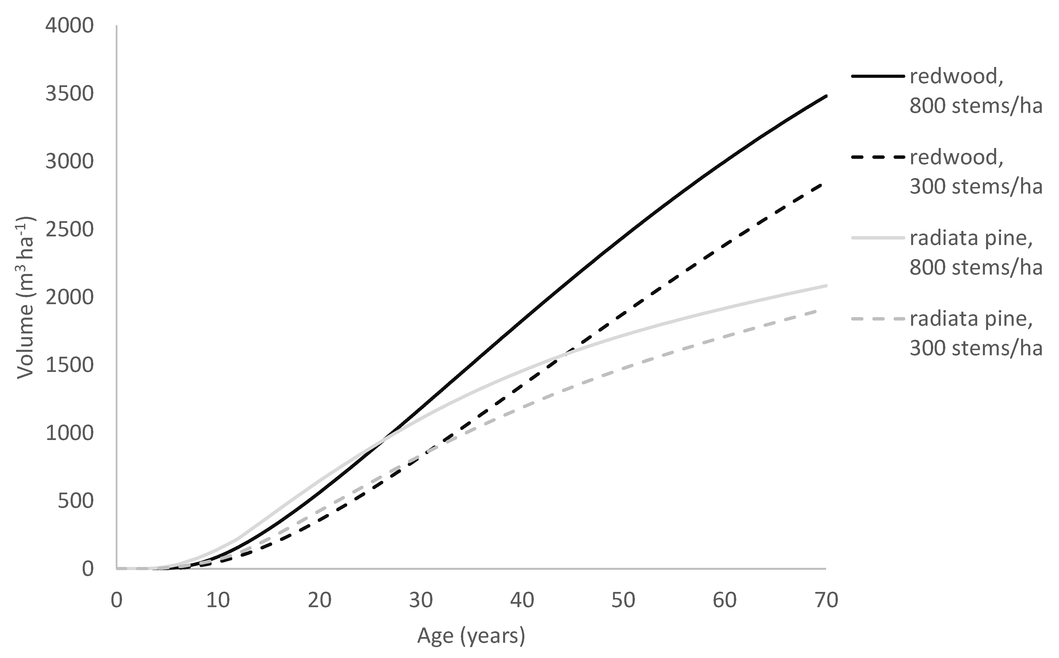
As a consequence, in trees showing similar early growth, those following the Richards growth pattern will slow more rapidly and approach the asymptote more abruptly than trees following the Korf growth pattern. Due to this, although the radiata pine model often predicts faster early growth than the redwood model does, it transitions towards its asymptote far more rapidly than the redwood model. 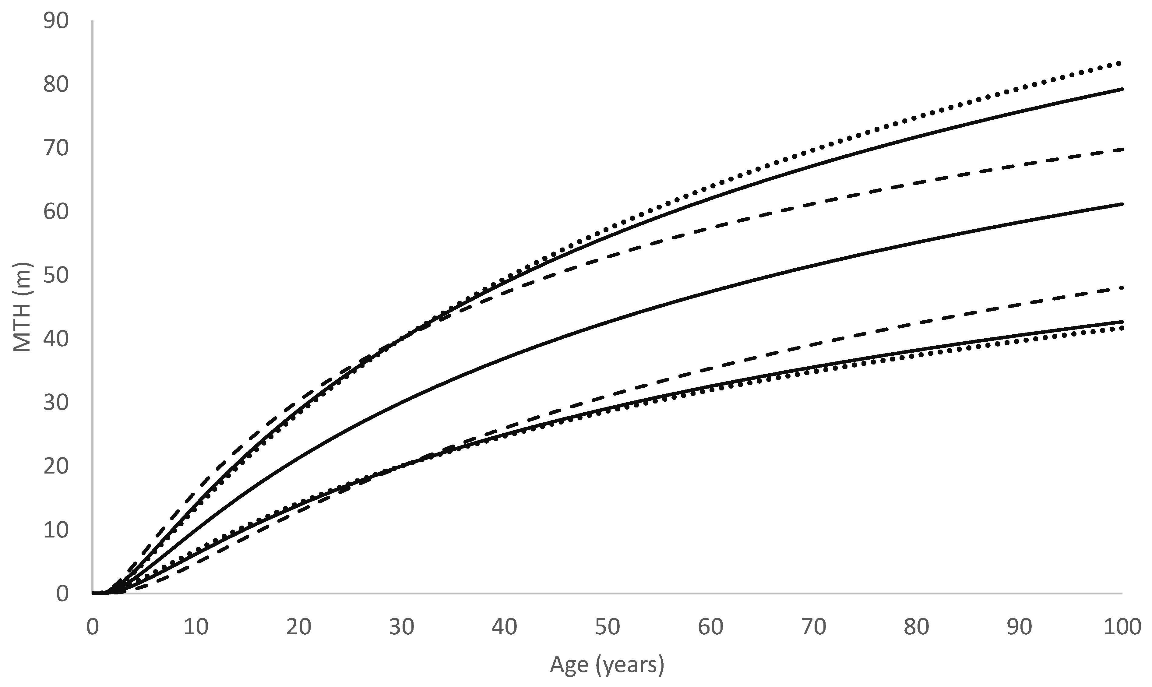This can be seen, for example, in Figure 9, which compares growth predictions by the two models for a site typical of the North Island of New Zealand. Although it may be premature to infer too much from only two species, these results suggest that the Richards model is better suited to modelling growth for fast-growing but relatively short-lived tree species such as radiata pine, whereas the Korf model performs better at modelling fast-growing but extremely long-lived species that can maintain high growth rates over a prolonged period such as redwood.

The growth model described in this paper can be used in similar ways to other empirical growth models. These include the projection of yield from inventory data and regime evaluation. The characterisation of a stand using the 300 Index and SI only requires a single measurement of age, stand density, MTH and BA. Following this characterisation, site productivity can be evaluated and metrics of stand growth can be predicted for any age and management regime. The model is therefore particularly well suited for regime evaluation, as once the two productivity indices have been determined for a forest, it can be used to assess the effects of stand density, the intensity and timing of thinning and rotation length on harvest production. The facility to accurately model tree growth under a variety of stand densities and thinning regimes, across a wide range of site qualities, is likely to substantially improve management of redwood within New Zealand.

Predictions made by this model can be used to produce regional maps describing variation in the 300 Index. As described above, the model can be readily used to estimate the 300 Index from sample plots, and this is likely to be particularly useful when plot data representing wide environmental gradients are available (e.g., national permanent sample plot datasets). By extracting environmental covariates for plot locations from GIS layers, regional models of the 300 Index can be created. Using this approach, a redwood 300 Index surface has been developed for New Zealand and compared to a previously produced 300 Index surface for radiata pine [36]. Results from this study show that redwood is more productive than radiata pine throughout most of the North Island [36]. Spatial comparisons of these surfaces are invaluable for growers who are purchasing new land or making decisions around species selection for new plantings. The 300 Index can also be used to examine historical trends in productivity and the response of stands to experimental treatments. The model of redwood 300 Index for New Zealand described above showed there was little variation in productivity for stands established prior to 1978, after which there was an exponential increase in 300 Index that continued through to the most recently planted stands in 2013 [36].

The development of national surfaces describing the 300 Index and SI also provides a useful means of model parameterisation which greatly enhances the generality of the model. Such a method is widely used within New Zealand for describing the productivity of radiata pine, and these national surfaces are part of the software used to parameterise growth for a specific site [24]. This approach can be used for running model simulations when plot data are not available. The linking of the growth model to these productivity surfaces effectively transforms the described empirical model into a hybrid model that is sensitive to fine-scale environmental variation.

5. Conclusions

This study describes a novel empirical growth modelling approach for New Zealand-grown redwood. Using the developed equations, the predictions closely matched time series measurements of key stand dimensions. This model will be of considerable use to growers for regime evaluation and prediction of yield, and the approach allows more precise estimation of site productivity than empirical growth models based only on SI. While the dataset used to develop the model was relatively limited, it did cover a wide range in site productivity as described by SI and 300 Index. Further research should, however, continue to test and refine the model as new measurement data become available.

References

1. Weiskittel, A.R.; Hann, D.W.; Kershaw, J.A.; Vanclay, J.K. Forest Growth and Yield Modeling; John Wiley & Sons: New York, NY, USA, 2011. [Google Scholar]
2. Korzukhin, M.D.; Ter-Mikaelian, M.T.; Wagner, R.G. Process versus empirical models: Which approach for forest ecosystem management? Can. J. For. Res. 1996, 26, 879–887. [Google Scholar] [CrossRef]
3. Larocque, G.R. Forest models. In Ecological Models Vol. [2] of Encyclopedia of Ecology; Sven, E.J., Brian, D.F., Eds.; Elsevier: Amsterdam, The Netherlands, 2008; Volume 5, pp. 1663–1673. [Google Scholar]
4. Bossel, H. Modeling and Simulation; Springer: New York, NY, USA, 2013. [Google Scholar]
5. Godfrey, K. Compartmental Models and Their Application; Academic Press: London, UK; New York, NY, USA, 1983. [Google Scholar]
6. Makela, A.; Landsberg, J.; Ek, A.R.; Burk, T.E.; Ter-Mikaelian, M.; Agren, G.I.; Oliver, C.D.; Puttonen, P. Process-based models for forest ecosystem management: Current state of the art and challenges for practical implementation. Tree Physiol. 2000, 20, 289–298. [Google Scholar] [CrossRef] [PubMed]
7. Kirschbaum, M.U.F.; Watt, M.S.; Tait, A.; Ausseil, A.G.E. Future wood productivity of Pinus radiata in New Zealand under expected climatic changes. Glob. Chang. Biol. 2012, 18, 1342–1356. [Google Scholar] [CrossRef]
8. Battaglia, M.; Sands, P.J. Process-based forest productivity models and their application in forest management. For. Ecol. Manag. 1998, 102, 13–32. [Google Scholar] [CrossRef]
9. Johnsen, K.; Samuelson, L.; Teskey, R.; McNulty, S.; Fox, T. Process models as tools in forestry research and management. For. Sci. 2001, 47, 2–8. [Google Scholar]
10. Salekin, S.; Mason, E.G.; Morgenroth, J.; Bloomberg, M.; Meason, D.F. Hybrid height growth and survival model for juvenile Eucalyptus globoidea (Blakely) and E. bosistoana (F. Muell) in New Zealand. For. Ecol. Manag. 2021, 490, 119074. [Google Scholar]
11. Pinjuv, G.; Mason, E.G.; Watt, M. Quantitative validation and comparison of a range of forest growth model types. For. Ecol. Manag. 2006, 236, 37–46. [Google Scholar] [CrossRef]
12. Rachid-Casnati, C.; Mason, E.G.; Woollons, R.C. Using soil-based and physiographic variables to improve stand growth equations in Uruguayan forest plantations. iForest-Biogeosciences For. 2019, 12, 237–245. [Google Scholar] [CrossRef] [Green Version]
13. Landsberg, J.J.; Johnsen, K.H.; Albaugh, T.J.; Allen, H.L.; McKeand, S.E. Applying 3-PG, a simple process-based model designed to produce practical results, to data from loblolly pine experiments. For. Sci. 2001, 47, 43–51. [Google Scholar]
14. Gupta, R.; Sharma, L.K. The process-based forest growth model 3-PG for use in forest management: A review. Ecol. Model. 2019, 397, 55–73. [Google Scholar] [CrossRef]
15. Skovsgaard, J.P.; Vanclay, J.K. Forest site productivity: A review of the evolution of dendrometric concepts for even-aged stands. For. Int. J. For. Res. 2008, 81, 13–31. [Google Scholar] [CrossRef] [Green Version]
16. Bontemps, J.-D.; Bouriaud, O. Predictive approaches to forest site productivity: Recent trends, challenges and future perspectives. Forestry 2014, 87, 109–128. [Google Scholar] [CrossRef]
17. Baur, F. Die Rothbuche in Bezug auf Ertrag, Zuwachs und Form: Unter Zugrundlegung der an der Kgl. Württemberg’schen Forstlichen Versuchsanstalt Angestellten Untersuchungen Bearbeitet; Verlag: Berlin, Germany, 1881. [Google Scholar]
18. Gyldenfeldt, W. En Tilvæxtoversigt for Bøg paa 2det Kjøbenhavn Distrikt. Tidsskr. Skovbrug 1883, 6, 1–46. [Google Scholar]
19. Eichhorn, F. Beziehungen zwischen bestandshöhe und bestandsmasse. Allg. Forst-und Jagdzetg. 1904, 80, 45–49. [Google Scholar]
20. Assmann, E. Die Bedeutung des „erweiterten Eichhorn’schen Gesetzes “für die Konstruktion von Fichten-Ertragstafeln. Forstwiss. Cent. 1955, 74, 321–330. [Google Scholar] [CrossRef]
21. Assmann, E. Höhenbonität und wirkliche Ertragsleistung. Forstwiss. Cent. 1959, 78, 1–20. [Google Scholar] [CrossRef]
22. Henriksen, H.A. Sitkagranens Vækst Og Sundhedstilstand I Danmark; Kandrup & Wunsch’s Bogtr: Copenhagen, Denmark, 1958; Volume 24. [Google Scholar]
23. Kennel, R. Die Bestimmung des Ertragsniveaus bei der Buche. Forstwiss. Cent. 1973, 92, 226–234. [Google Scholar] [CrossRef]
24. Kimberley, M.O.; West, G.; Dean, M.; Knowles, L. Site Productivity: The 300 Index—A volume productivity index for radiata pine. N. Z. J. For. 2005, 50, 13–18. [Google Scholar]
25. Hasenauer, H.; Burkhart, H.E.; Sterba, H. Variation in potential volume yield of loblolly pine plantations. For. Sci. 1994, 40, 162–176. [Google Scholar]
26. Vanclay, J.K.; Skovsgaard, J.P.; Hansen, C.P. Assessing the quality of permanent sample plot databases for growth modelling in forest plantations. For. Ecol. Manag. 1995, 71, 177–186. [Google Scholar] [CrossRef] [Green Version]
27. Skovsgaard, J.P. Management of Sitka spruce without thinnings: An analysis of stand structure and volume production of unthinned stands of Sitka spruce (Picea sitchensis (Bong.) Carr.) in Denmark. Forskningsserien. Forskningscentret Skov og Landsk. (Den.) 1997, 19, 529. [Google Scholar]
28. Schmidt, A. Ertragsniveau und Standort dargestellt am Beispiel der Kiefer. Forstwiss. Cent. 1973, 92, 268–274. [Google Scholar] [CrossRef]
29. Bailey, R.L.; Clutter, J.L. Base-age invariant polymorphic site curves. For. Sci. 1974, 20, 155–159. [Google Scholar]
30. Cieszewski, C.J.; Bailey, R.L. Generalized algebraic difference approach: Theory based derivation of dynamic site equations with polymorphism and variable asymptotes. For. Sci. 2000, 46, 116–126. [Google Scholar]
31. Zeide, B. Analysis of growth equations. For. Sci. 1993, 39, 594–616. [Google Scholar] [CrossRef]
32. Brown, J.E. Monarchs of the Mist: The Story of Redwood National Park and the Coast. Redwoods; Coastal Parks Association: Point Reyes, CA, USA, 1982. [Google Scholar]
33. Earle, C.J. Sequoia Sempervirens. The Gymnosperm Database. 2018. Available online: https://www.conifers.org/cu/Sequoia.php. (accessed on 11 March 2021).
34. Sillett, S.C.; Van Pelt, R.; Carroll, A.L.; Campbell-Spickler, J.; Antoine, M.E. Aboveground biomass dynamics and growth efficiency of Sequoia sempervirens forests. For. Ecol. Manag. 2020, 458, 117740. [Google Scholar] [CrossRef]
35. Watson, F.D. Sequoia sempervirens. In Flora of North America Editorial Committee; Flora of North America North of Mexico (FNA). 2. New York and Oxford. Retrieved 1 February 2015—Via eFloras.org; Missouri Botanical Garden: St. Louis, MO, USA; Harvard University Herbaria: Cambridge, MA, USA, 1993. [Google Scholar]
36. Watt, M.S.; Kimberley, M.O.; Rapley, S.; Webster, R. Comparing volume productivity of redwood and radiata pine plantations in New Zealand. For. Ecol. Manag. 2021, in press. [Google Scholar]
37. NZFOA. 2019/2020 Facts and Figures. In New Zealand Plantation Forest Industry; New Zealand Forest Owners Association: Wellington, New Zealand, 2020; Available online: https://www.nzfoa.org.nz/images/Facts_Figures_2019_20_Web_FA3-updated.pdf (accessed on 23 July 2021).
38. Rapley, S. Redwood in New Zealand. N. Z. J. For. 2018, 63, 29–33. [Google Scholar]
39. R Development Core Team. R: A Language and Environment for Statistical Computing; R Foundation for Statistical Computing: Vienna, Austria, 2011. [Google Scholar]
40. Richards, F.J. A flexible growth function for empirical use. J. Exp. Bot. 1959, 10, 290–300. [Google Scholar] [CrossRef]
41. Korf, V. Příspevěk k matematické formulaci vzrůstového zákona lesních porostů. [Contribution to mathematical definition of the law of stand volume growth]. Lesnická Práce 1939, 18, 339–379. [Google Scholar]
42. Kimberley, M.O.; Beets, P.N. National volume function for estimating total stem volume of Pinus radiata stands in New Zealand. N. Z. J. For. Sci. 2007, 37, 355–371. [Google Scholar]
43. Berrill, J.-P.; O’Hara, K.L. Estimating site productivity in irregular stand structures by indexing the basal area or volume increment of the dominant species. Can. J. For. Res. 2014, 44, 92–100. [Google Scholar] [CrossRef]
44. Berrill, J.-P.; O’Hara, K.L. How do biophysical factors contribute to height and basal area development in a mixed multiaged coast redwood stand? Forestry 2016, 89, 170–181. [Google Scholar] [CrossRef]
45. van der Colff, M.; Kimberley, M.O. A National height-age model for Pinus radiata in New Zealand. N. Z. J. For. Sci. 2013, 43, 4. [Google Scholar] [CrossRef] [Green Version]
46. Garcia, O. New class of growth models for even-aged stands: Pinus radiata in Golden Downs forest. N. Z. J. For. Sci. 1984, 14, 65–88. [Google Scholar]
47. García, O. The state-space approach in growth modelling. Can. J. For. Res. 1994, 24, 1894–1903. [Google Scholar] [CrossRef]
48. García, O. Height growth of Pinus radiata in New Zealand. N. Z. J. For. Sci. 1999, 29, 131–145. [Google Scholar]
Figure 1. Geometry of Equation (2) showing Dq predicted for stand densities of 200, 300, 500 and 800 stems ha−1. Line A is y = D(tBH), which is Dq at a stand density of 300 stems ha−1. The dashed line B is y = kg + (1 − k)D(tBH), where k = d(ln800 − ln300), which intersects line A at y = g. The solid line C produced by a stand density of N = 800 stems ha−1 initially follows line A but then transitions towards line B.
Forests 12 01155 g001
Figure 2. Diagram showing how Dq is modelled in the redwood growth model for a stand thinned from 800 to 300 stems ha−1 at age 30 years. The dashed line A is Equation (2) for a stand density of 300 stems ha−1 and the dotted line B is Equation (2) for a stand density of 800 stems ha−1. The solid line C shows Dq for the thinned stand. It follows line B until the thinning event, when thinning selection generally causes an immediate increase in Dq. Thereafter, the thinned stand maintains a horizontal separation from line A equal to Δtthin, increasing slightly to Δtthin+0.25 after one year to allow for crown expansion following thinning.
Forests 12 01155 g002
Figure 3. Comparison of the polymorphic form of the Korf model (solid lines) with the anamorphic (dotted lines) and common asymptote (dashed lines) forms, fitted to the redwood MTH data. The central solid line is for SI = 30 m, the three lower lines are for SI = 20 m and the upper three lines are for SI = 40 m.
Forests 12 01155 g003
Figure 4. Mean top height vs. age for data from measured stands. Grey dots indicate measurements, with grey solid lines showing plots measured multiple times. Black lines show predictions from Equation (15) based on the initial measurement in each plot.
Forests 12 01155 g004
Figure 5. Quadratic mean DBH vs. age for the plot measurement database. Grey dots indicate measurements, with grey solid lines showing plots measured multiple times. Black lines show predictions from Equation (18) based on the initial measurement in each plot.
Forests 12 01155 g005
Figure 6. Mean stand density vs. age for the plot measurement database. Grey dots indicate measurements, with grey solid lines showing plots measured multiple times. Black lines show predictions from Equation (9) based on the initial measurement in each plot.
Forests 12 01155 g006
Figure 7. Stem volume vs. age for the plot measurement database. Grey dots indicate measured volumes, with grey solid lines showing plots measured multiple times. Black lines show predictions from the growth model based on the initial measurement in each plot.
Forests 12 01155 g007
Figure 8. Plots of predicted against measured values for (a) volume, (b) mean top height, (c) diameter at breast height and (d) stand density. Plots with two or more repeated measurements were included, and the last prediction for each plot is shown. The 1:1 line is denoted by the solid black line, while the solid red line shows a linear relationship of best fit through the data.
Forests 12 01155 g008
Figure 9. Stem volume predictions from the 300 Index growth models for redwood and radiata pine at 800 and 300 stems ha−1 for a typical New Zealand North Island site with 300 Index = 27.5 m3 ha−1 yr−1 for both species.
Forests 12 01155 g009