Evaluating the Capability of Unmanned Aerial System (UAS) Imagery to Detect and Measure the Effects of Edge Influence on Forest Canopy Cover in New England

Abstract

Characterizing and measuring the extent of change at forest edges is important for making management decisions, especially in the face of climate change, but is difficult due to the large number of factors that can modify the response. Unmanned aerial systems (UAS) imagery may serve as a tool to detect and measure the forest response at the edge quickly and repeatedly, thus allowing a larger amount of area to be covered with less work. This study is a preliminary attempt to utilize UAS imagery to detect changes in canopy cover, known to exhibit changes due to edge influences, across forest edges in a New England forest. Changes in canopy cover with increasing distance from the forest edge were measured on the ground using digital cover photography and from photogrammetric point clouds and imagery-based maps of canopy gaps produced with UAS imagery. The imagery-based canopy gap products were significantly more similar to ground estimates for canopy cover (p value > 0.05) than the photogrammetric point clouds, but still suffered overestimation (RMSE of 0.088) due to the inability to detect small canopy openings. Both the ground and UAS data were able to detect a decrease in canopy cover to between 45–50 m from the edge, followed by an increase to 100 m. The UAS data had the advantage of a greater sampling intensity and was thus better able to detect a significant edge effect of minimal magnitude effect in the presence of heavy variability.

1. Introduction

Forest fragmentation is an increasingly pervasive problem that threatens global biodiversity and decreases ecosystem services by degrading habitat quality [1,2,3,4]. After removal, the remaining forest is exposed to the surrounding land cover matrix, leading to edge influences (EI), the effect of abiotic and biotic processes at the edge [3,4]. Edge habitat is the area over which EIs are having a significant impact on forest condition. In general, there is greater light availability, temperature variability, and wind as well as increased access to organisms and materials such as pollen and seeds immediately following the edge creation [5,6,7,8,9]. These direct effects of edge creation influence ecological processes (e.g., productivity, evapotranspiration, decomposition, recruitment, and mortality), which lead to changes in the forest structure [10,11,12,13]. These modifications at the edge can make the area less suitable for many of the species that once resided in and/or relied on the interior forest habitat (i.e., core area), effectively making the remaining forest patch smaller for them to survive in [4,14]. The composition at the edges of forest patches has been found to shift toward edge-adapted, typically early-successional species in many parts of the world [15,16,17]. As fragmentation continues, patches become smaller and more irregularly shaped, causing them to be increasingly dominated by edge habitat [4,18].

Understanding the impacts of fragmentation and the relative amount of core and edge forest habitat on the landscape requires an understanding of how far into a forest patch the edge is exerting an influence [19,20,21,22]. A first step in accomplishing this is to estimate the depth of edge influence (DEI) [18,23] or the distance from the edge into the forest community over which there is a substantial EI [3]. Once known, edge habitat on the landscape scale can be modeled [21,22]. DEI is typically determined in the field by sampling along the edge to interior gradient. Transects running perpendicular from the forest edge into the interior with systematic sampling plots placed at known intervals from the edge are commonly established [8,11,17,24,25,26]. At each plot, one or more variables related to forest structure, composition, or processes that are believed to co-vary with distance from the edge are measured (see Harper et al. [3] for review). Potential “edge samples” are compared to reference samples that are believed to represent interior forest conditions [11,12,27,28,29]. The DEI is measured as the sample (i.e., distance) farthest from the edge that is considerably different from the interior.

DEI is a highly variable number, however, and has been found to vary with edge maintenance (i.e., is regeneration suppressed via mowing or plowing), landscape orientation, age, and stand composition [5,9,13,30]. A current review of forest edge research has further found a great deal of variation across forest biomes and edge origin (natural vs. anthropogenic) [31]. One-size-fits-all DEI for landscape modeling is not appropriate [32], assuming a singular DEI has important implications when planning conservation areas or developing management plans with interior forest preservation in mind [21,32,33]. Additionally, the structure of the forest at the edge may have implications on modeling global carbon balances [34,35] However, this variability makes it difficult to accurately measure edge depth at this scale without extensive fieldwork [36,37]. Moreover, it is becoming more important to assess the temporal changes across these edges in the face of climate change [9,34], making repetitive collections necessary.

Measures of forest structure, commonly used in studies of edge influences to describe forest edge habitats, have been made from remotely sensed data for decades [38]. Remotely sensed data such as satellite or aerial imagery and LiDAR have the benefit of covering large areas with repeat visitation. Given this advantage, several studies have attempted to make use of these data for investigating edge influences assessing changes in remotely sensed estimates of structure with distance. MacLean [37] and Vaughn et al. [39] utilized LiDAR to estimate changes in understory and overstory canopy cover, respectively, and found significant relationships between edge distance and cover. Dantas De Paula et al. [36] utilized a Landsat Tree Cover dataset [40] to investigate changes in canopy cover with distance from a forest edge at 11 study sites across five continents, finding significantly lower canopy cover near edges across all sites. These studies demonstrate the usefulness of remotely sensed data for investigating edge influences. However, LiDAR data can be expensive to collect, outdated, or lacking the specifications (e.g., spatial resolution and leaf-on imagery) necessary to appropriately measure EIs [41,42,43]. Additionally, the LANDSAT Tree Cover data or similar image products such as the National Land Cover Data (NLCD) Tree Cover dataset (https://www.mrlc.gov/finddata.php, accessed on 15 July 2021) are mapped at a 30 m spatial resolution. At this resolution, a pixel will cover the extent of most measured edge effects [3].

Imagery collected by unmanned aerial systems (UAS) have become a flexible and cost-effective means of gathering forest structural information. Recent advancements in computer vision, combined with well-established photogrammetric techniques, have led to two processes known as structure-from-motion (SfM) [44] and multi-view stereo (MVS), typically abbreviated SfM-MVS because they are often both employed together. These processes allow similar three-dimensional information to be extracted from imagery collected by inexpensive digital cameras [45]. When the sensor is mounted on a UAS, the combination becomes a powerful tool for studying forests [46]. Highly dense point clouds similar to that of LiDAR data can be produced from overlapping UAS images. While it lacks the ability to capture more of the forest’s internal vertical structure [47,48,49,50], UAS imagery can capture measures of canopy cover [47,51]. Canopy cover has commonly been found to experience substantial effects due to EI [5,8,12,24,52] and is important ecologically, as it controls a number of biotic and abiotic processes on the ground [53,54]. The high spatial resolution orthomosaics, with spatial resolution on the order of centimeters, produced from the UAS imagery have also been utilized to estimate foliage cover [54,55,56,57], although comparisons between cover estimates generated from the photogrammetric point clouds and orthomosaics are lacking. To date, no study has utilized the products of UAS imagery to investigate edge influences. If found to be a successful tool, the flexibility of the UAS could significantly increase data collection at the edge, especially over time due to its ability to collect imagery wherever and whenever needed at a fraction of the cost, relative to aerial or satellite imagery [58].

More attention needs to be paid to the structure of the edges in New England, and more generally, the eastern US temperate broadleaved forests, as they can potentially be important for carbon sequestration [59]. Understanding the effects on forests at these edges can better inform our carbon accounting [31,34]. The forests of New England are relatively young due to human modification following colonial settlement [60,61,62,63]. In general, a considerable amount of the region was completely deforested for agriculture and remained that way until they were abandoned and left to regenerate by the late 19th century [64,65]. This has resulted in young forests not yet facing age-related declines in growth rate and a number of disturbance-adapted species present in the area that can take advantage of the increased resources at the edges [66].

New Hampshire, a part of the New England region in the US, has long maintained the title of being the second most forested state in the US. However, recent data shows that the state has been experiencing a continuous decrease in forest cover [60,61,62]. The increase in development due to population growth has led to the fragmentation of large forest blocks with more predicted to occur in the future [63], resulting in increasing exposure to edge influences. Therefore, the objective of this study was to investigate whether UAS imagery could be used to detect and assess the depth of edge influence in a New Hampshire forest. We focused on changes in canopy cover due to its strong influence on other aspects of forest structure [3]. The measurements of canopy cover extracted from the UAS imagery were compared to ground-based measurements to determine feasibility of this method. The effects of edge influences were then modeled using both the ground and UAS-generated data to characterize and quantify the effect, if present. This study serves as an initial assessment of UAS for assessing edge habitats and should spur additional research into the effects that can be quantified with this technology.

2. Materials and Methods

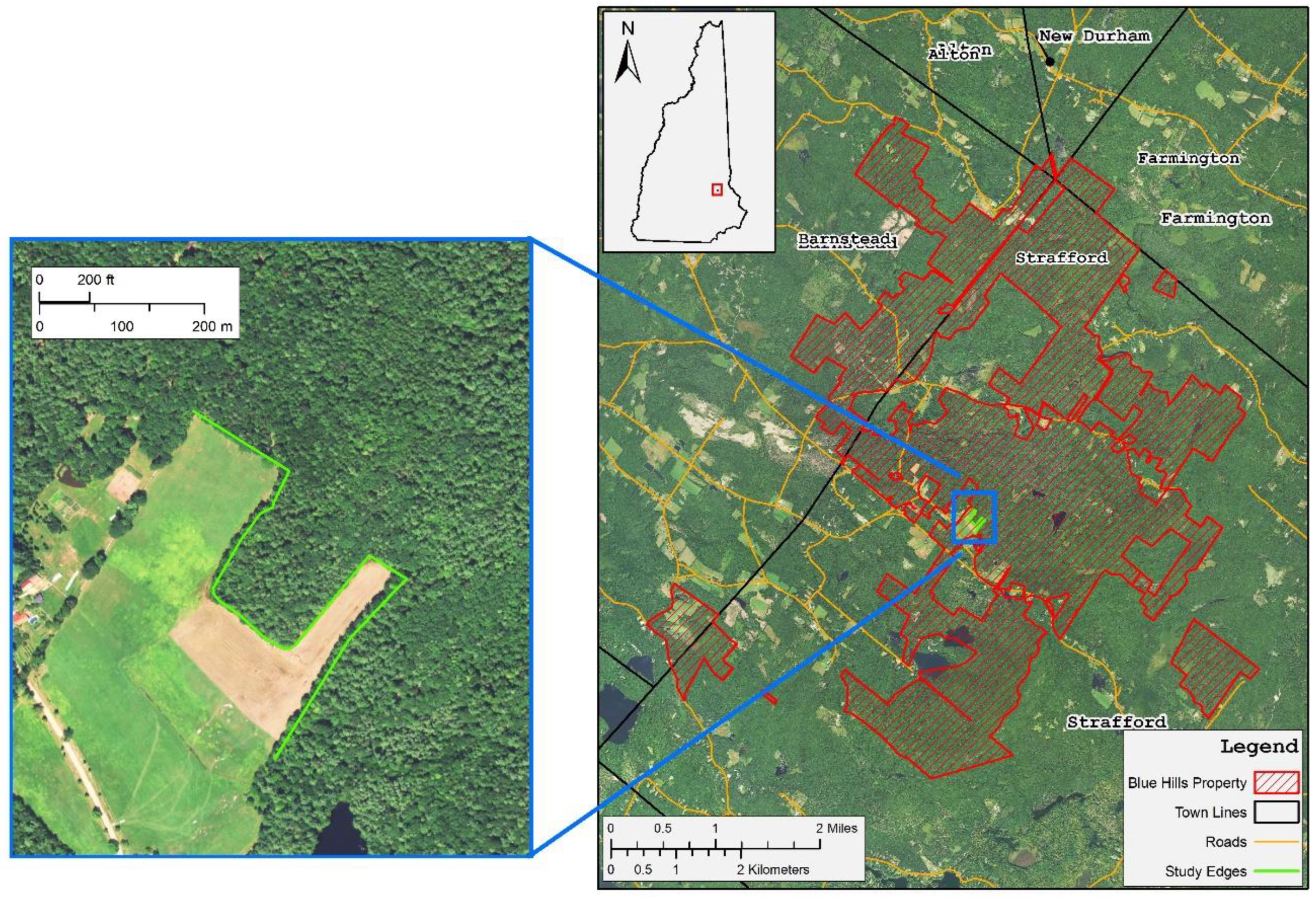
2.1. Study Area

This research was conducted on the Blue Hills Foundation conservation lands in New Hampshire, USA (Figure 1). The area covers 2946.95 ha and spans five New Hampshire towns. This property is owned by the Blue Hills Foundation Inc. and managed by the Harvard Forest. This stand represents a natural, highly mixed, transition hardwood-hemlock-white pine forest community as described by Westveld [67] or a Hemlock-beech-oak-pine forest as discussed in Sperduto and Nichols [68]. White pine (Pinus strobus) and eastern hemlock (Tsuga canadensis) are the dominate species in the forest followed by red maple (Acer rubrum), red oak (Quercus rubra), red pine (Pinus resinosa), and American beech (Fagus grandifolia). Our study site and corresponding edges were carefully selected due to their proximity to a suitably sized field for UAS flying and adjacency to continuously maintained fields because it represents a predominately southern edge exposure, and because these edges are considered older (>30 years old) [3].

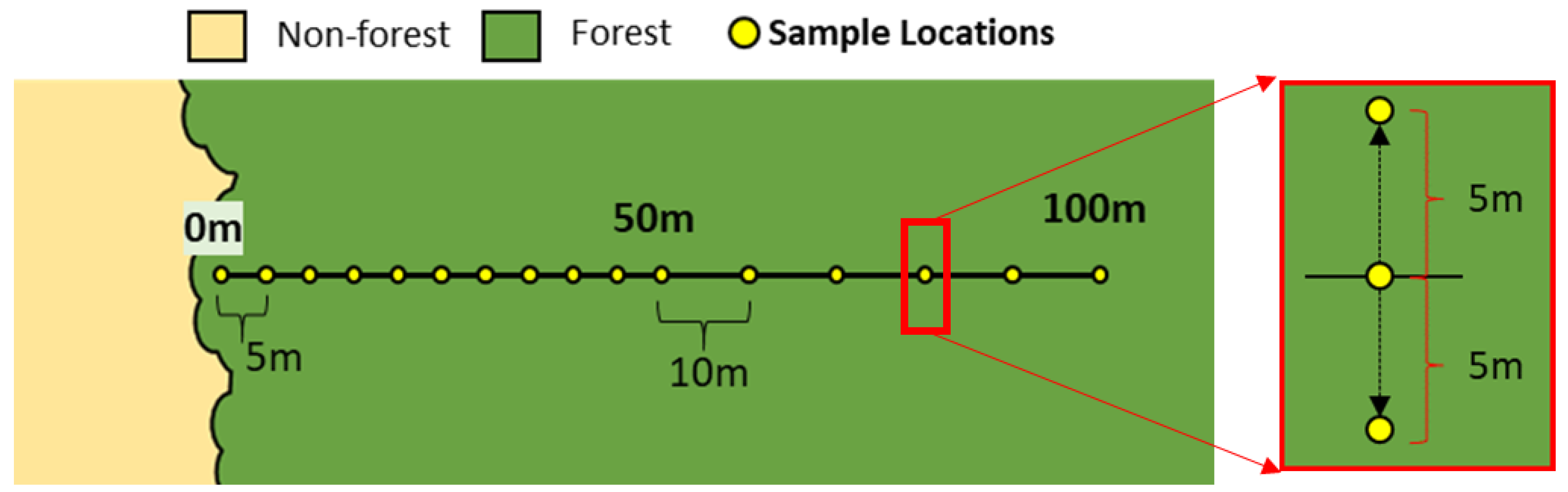
2.2. Ground Data Collection

To establish a reference for the edge effects in the study area, a traditional ground data collection of foliage cover (i.e., the vertical projection on the ground of the forest canopy including within crown gaps) was conducted. Ground data was collected between 28 September 2019 and 30 September 2019. Nine transects running perpendicular into the forest were established along an approximately 944 m length of forest edge. A random point along this edge was chosen for the placement of the first transect. Subsequent transects were spaced 100 m apart and/or >50 m from a corner [8,10,24,25]. Figure 2 shows the general sampling setup along each transect. The transect bearing was chosen as the azimuth perpendicular to the edge with the 0 m distance point placed on the edge line. The edge line was considered the inside edge of any stone walls if present, or the outermost extent of the tree stems within roughly 10 m of either side of the transect location. Once the starting position and bearing were established, sampling locations were placed systematically along the transect line. Sample spacing was 5 m within the first 50 m and then was increased to 10 m between 50 m–100 m. The sampling intensity was higher up to 50 m because edge effects have commonly been found to extend 50 m or less into the forest [3,5,37,69]. Not every transect line extended 100 m out. Transect distance alternated between 50 and 100 m except in the case where a 100 m distance would place the end of the transect within 50 m of a second edge. In addition to a sample point being taken along the transect line at the specified distance interval, two more samples were taken 5 m perpendicular on either side of the centered point. Thus, for each distance, three samples were collected.

Digital cover photography (DCP) was employed to estimate the foliage cover (FC) at each sample location [70,71] (Figure 3). DCP is similar to traditional digital hemispherical photography but utilizes a much narrower field of view (0–30° compared to 0–180°). A predominantly vertical image of the canopy was collected and then processed to separate the sky from everything else. FC was calculated as the percentage of the image not considered sky. DCP is more robust to camera parameters, lighting conditions, produces higher resolution images [72], and has been found to accurately measure foliage cover [72,73,74]. Digital canopy photos were collected at each sample site using a Canon Rebel T6i mounted to a 4 m tall extension pole to capture only the upper canopy. The focal length was set to 55 mm, which is approximately a 15.42° field of view. For each picture, the pixels were classified as either sky or vegetation using the procedures outlined in Nobis and Hunkiker [75]. FC for each image was simply the proportion of that image classified as vegetation. The three FC measurements taken at each distance on each transect were then averaged together.

2.3. UAS Data Collection and Processing

UAS imagery was collected over the study area on 1 July 2020 with a Sensefly eBee X fixed-wing and the eMotion 3 mission planning software [76]. The Sensefly Aeria X camera was used to collect the imagery. The Aeria X is a standard DSLR camera and captures high-resolution (24 megapixel) natural color (RGB) imagery. The weather this day was calm winds and predominately overcast, which helped to maintain consistent illumination across all the images. The imagery was collected 100 m above the trees (approximately 120 m above the ground) with an 80% and 85% latitudinal and longitudinal overlap, respectively. The mission area for each edge of the study site was set up to collect at least 200 m from the edge into the forest. In total, 1299 images were collected and used to generate the following UAS-derived products.

The eBee X is real-time kinematic (RTK) enabled; thus, the raw GPS positions for each image were post-process kinematic (PPK) corrected using the Sensefly Flight Data Manager included with the eMotion 3 mission planning software. Resulting positional accuracy following PPK processing was around 7 cm. The UAS images were then processed in Agisoft Metashape Professional [77]. Agisoft utilizes the SfM and MVS processes to produce dense, photogrammetrically generated point clouds and orthomosaics. While a full explanation of the process is beyond the scope of this paper, the point clouds are produced by automatically matching features across the multiple overlapping images and using the estimated camera interior and exterior orientation to estimate the absolute coordinate position and height for each matched feature (i.e., point). A digital surface model (DSM) was produced from the resulting point cloud, which was then used to orthorectify the UAS images. The rectified images were then mosaiced together to produce an orthomosaic. The specific Agisoft processing parameters were: (1) Align Photos run with “high accuracy” and generic preselection, guides image matching, and adaptive model fitting turned on; (2) The dense point cloud generation was run on “ultra-high” quality and mild filtering; (3) The UAS imagery was ortho rectified using a DSM generated from the dense point cloud and mosaicked. The dense point cloud (density of 8264 pts/m²) and the orthomosaic were exported from Agisoft. The spatial resolution of the orthomosaic was 2.48 cm, however, for simplicity; they were exported at a 2.5 cm resolution such that the spatial resolution would be a factor of the plot sizes utilized in this study. The 2 mm difference was expected to have minimal impact on the canopy mapping below.

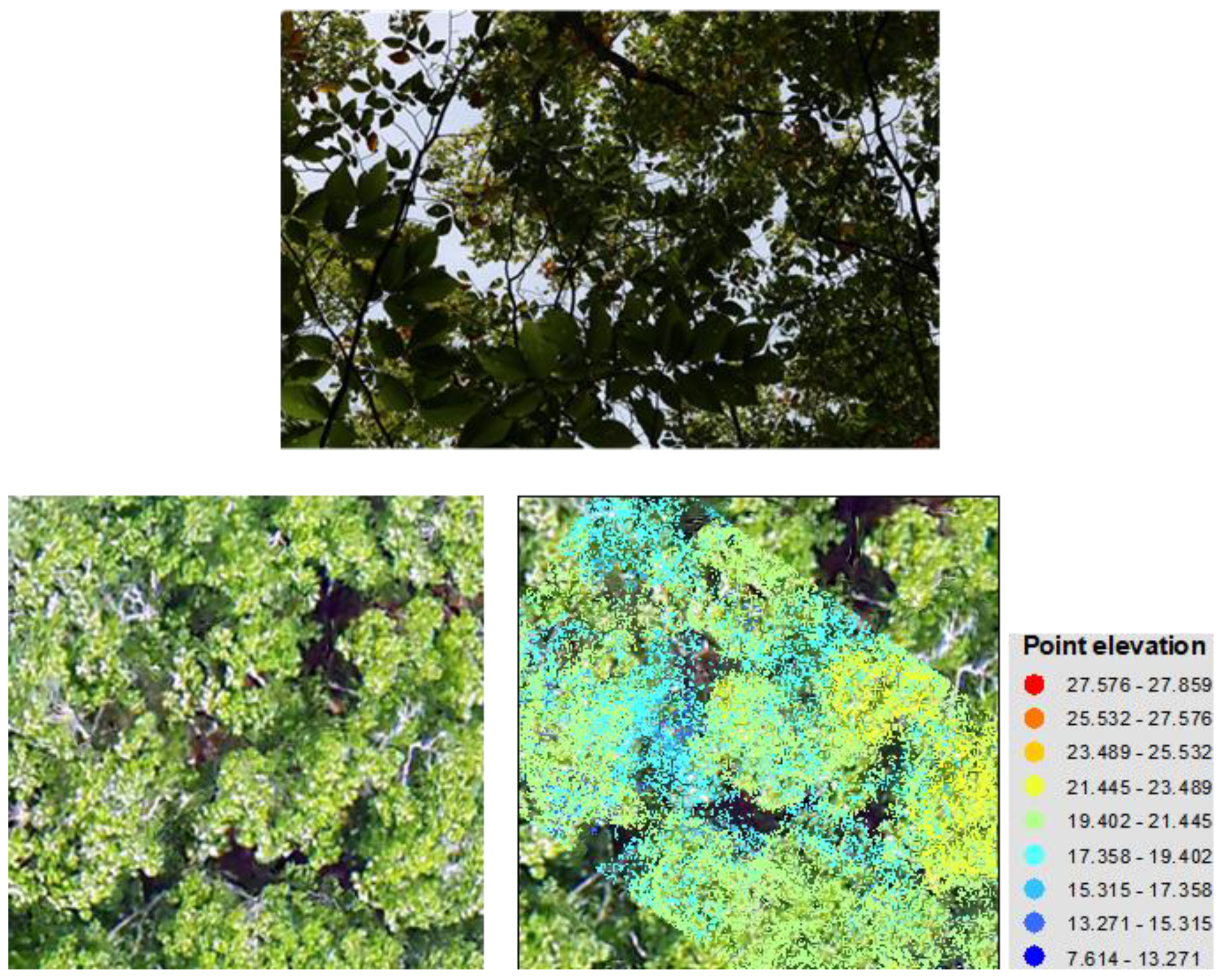
2.4. Estimating Foliage Cover from UAS Data Products

FC can be estimated two ways. The first is from the point cloud after normalizing the point elevations to height above the ground. The percentage of the points above a certain height threshold within a defined area were taken as an estimate of foliage cover. The second is an image-based method where the orthomosaic is used to map openings in the canopy creating a binary “gap map”. Similar to the point clouds, the percentage of a defined area not classified as a gap is the estimated FC. Both methodologies were employed in this study: first using the UAS point cloud and then the orthomosaic.

In the first approach, the dense point cloud was normalized to height above the ground using a digital terrain model (DTM) produced in 2015–2016 from leaf-off LiDAR data. Photogrammetrically produced point clouds typically lack points at the ground to generate an accurate DTM, especially over dense canopies. Thus, externally produced DTMs from LiDAR are often used to normalize them [78,79,80]. The DTM was downloaded from the GRANIT LiDAR distribution site (https://LiDAR.unh.edu/map/, last accessed on 15 July 2021) at a 1 m spatial resolution. The elevation of the ground estimated at the pixel within which each point fell was simply subtracted from the elevation of the point.

For the second image-based approach, a binary map representing gaps or openings in the canopy were mapped from the orthomosaic using a variation on the method developed by Macfarlane and Ogden [81] and was found to be well suited for estimating cover in dense forest stands [55,82]. This method splits the pixels in the orthomosaic into four training groups using logical rules based on the RGB pixel values. The groups of primary importance are the foreground and background pixels representing vegetation and non-vegetation, respectively. The orthomosaic is then transformed from the RGB color space to the CIE L*a*b* color space. The new bands represent a pixel’s luminosity (L), hue between magenta and green (a*) and hue between yellow and blue (b*). The separation of the luminance from the pixel color helps to avoid problems associated with uneven illumination across an image [83]. Additionally, the green leaf area (GLA) vegetation index was derived from the original RGB orthomosaic. The mean GLA, a*, and b* of the foreground and background groups is calculated. The pixels are then classified as either foreground or background using a minimum distance to the group mean classifier. Based on the work of Chianucci et al. [55], the pixels classified as foreground (vegetation) were considered the canopy while the background (non-vegetated) were considered the gaps.

The initial LAB2 results were adjusted to account for forest floor vegetation visible in canopy gaps, which should not be considered as part of the upper canopy. Additionally, tree limbs and overexposed canopy pixels were classified as non-vegetated due to having no green reflectance and being spectrally saturated across the RGB bands, respectively, but were part of the upper canopy. An assumption was made that objects in the upper canopy classified as “non-vegetation” would be bright (high L values relative to non-vegetated pixels below the canopy). Conversely, vegetation not in the upper canopy would be dark (lower L relative to real canopy vegetation). To account for this effect, a different threshold was applied to each group of pixels (vegetation vs. not vegetation) based the histogram of the L values for each. Threshold values were determined by looking for obvious breaks in the distributions. The result was similar to the LAB2 map but now considered gaps with vegetation in addition to the non-vegetated components and saturation errors above. These maps alone are not an estimate of FC but are used to estimate FC by summarizing the amount of gap within a defined area.

The effectiveness of the point cloud versus image-based (using the gap maps) method for estimating FC were assessed by comparing the FC estimates from method to the ground-measured FC from the DCP at the sample locations. Polygons of size 15 × 5 m centered along the transects at each measured distance were generated using the GPS positions collected during ground data collection and GIS. The width of these polygons was chosen to account for the maximum distance between the outside sample plus several meters to account for the fact that the DCP imagery at the outside samples would extend to the left and the right of the sample positions. Unfortunately, the exact area covered by a DCP image will vary considerably with upper canopy and mid-canopy height. The accuracy of GPS positions was often highly degraded when working under the dense forest cover. For this reason, only the starting position of each of the transects, the 0 m point, were recorded in the field. A Trimble Yuma, running Trimble TerraSync, was set up on a tripod in the adjacent field, away from the canopy edge with a clear view of the sky. The azimuth direction and distance from the GPS to the 0 m point was recorded. The unit was set to record its position at a 1 s sampling rate during the collection of the transect. These GPS positions were then PPK corrected in Trimble Pathfinder Office (positional error between 1–2 m), and using the azimuth and direction, utilized to calculate the coordinates of the 0 m point for each transect. The coordinates of the remaining sample locations were estimated using the distance along the transect from 0 m and the transect bearing. Only the points on the transect were estimated. The sample points on either side of the transect were not. The 15 × 5 m polygons were centered on each point. Thus, at any given location, the polygon extended 2.5 m north and south and 7.5 m east and west. The FC was calculated within each polygon first with the normalized point cloud and then by using the imagery-based gap maps. For the point cloud-based FC estimates, a 4 m threshold was used. This value was chosen to match the height above the ground; the DCP imagery was collected in the field. For comparison, FC with both the original LAB2 gap map and the modified LAB2 gap were calculated. The root mean squared error (RMSE) was calculated as a measure of similarity and statistically compared with a paired t test (alpha = 0.05).

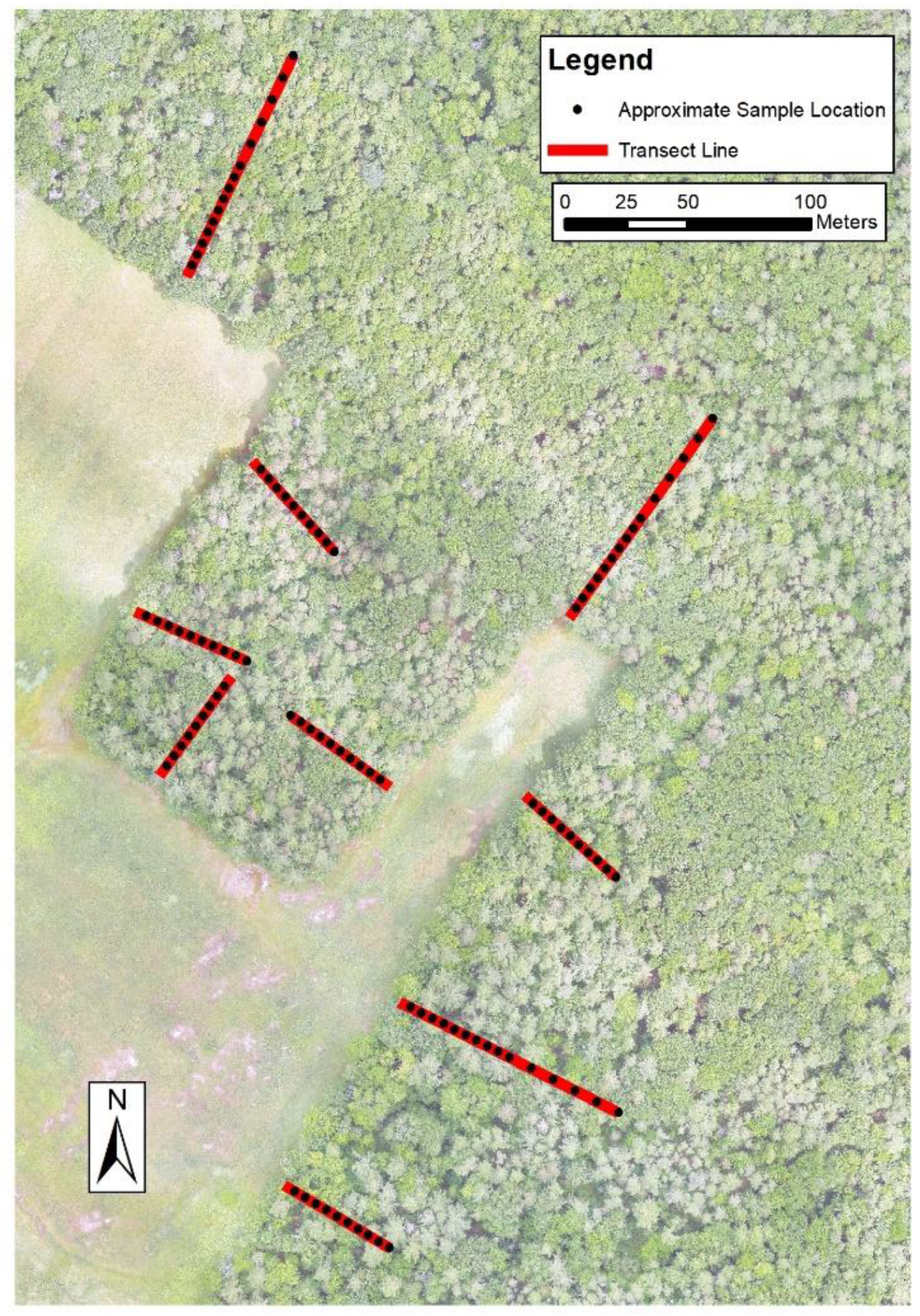
2.5. Investigating Edge Effects with UAS Data

Based on the results of the FC estimate comparison, the detection and modeling of edge effects using UAS data were conducted with modified LAB2 canopy gap maps. The edge line was digitized using leaf-off UAS imagery of the study site such that the edge under cantilevered canopies could be seen (See inset on Figure 1). Every effort was made to mimic the edge line rules applied during field collection. For simplicity, the digitized lines were generalized to minimize the number of vertices. A grid of points with a 5 m spacing oriented to the general bearing of the digitized edge line was produced. Only those points within 200 m of the edge were retained. A maximum distance of 50 m was applied to the edges along the convex portion of forest in the lower edge since this area is narrow. A 2.5 m radius buffer (5 m diameter) was placed around each point and the perpendicular distance and bearing from the centroid to the nearest edge line, not vertex, was calculated. The FC within each 5 m diameter buffer was then estimated using the canopy gap map.

2.6. Data Analysis

Generalized additive models (GAMs) [84] were used to determine where there was a significant relationship between FC and distance from an edge as well as to visualize the relationship, if present. GAMs are a powerful tool for modeling the often non-linear responses exhibited by edge effects and allows us to clearly visualize the trend between response and predictors [9,85,86,87]. Unlike generalized linear models (GLM), the assumption of a linear relationship between the response and a predictor variable is relaxed and is instead modeled as smooth, non-parametric function determined by fitting splines to the data. The analysis was conducted in R 4.0.2 [88] using the mgcv package [84]. The GAM was fit using the image-based FC estimates. FC was modeled as a smooth function of distance from edge, fitted using penalized cubic splines. Within the specific smooth function, k, the basis dimension or maximum degrees of freedom the smooth function is allowed to utilize, was set to 10. Per the suggestion of Wood [84], k should be large enough to ensure the underlying relationship is captured but low enough to maintain computational efficiency. The restricted maximum likelihood (REML) method was used to estimate the smoothing parameter for the model. The smooth parameter effectively reduces the degrees of freedom to avoid overfitting. Because FC represents proportions bounded between zero and one, a beta distribution and logit link function was specified. A built-in check of the basis dimension was run to ensure k was set high enough. Additionally, the standard residual diagnostic plots were scrutinized to ensure the standard model assumptions were met.

A spatial term to account for spatial autocorrelation was not included in the model. A semivariogram of deviance in FC by distance between adjacent samples was checked and little to no spatial autocorrelation in the sample data was found. This is consistent with the suggestion of Jennings [89] that the sample distance be greater than the largest tree crowns in order to reduce and avoid spatial autocorrelation between estimates of canopy cover. The 5 m spacing between samples is wider than the average tree crown in this stand.

3. Results

3.1. Ground Data Collection

In total, nine transects were measured on the ground (Figure 4). All transects extended at least 50 m into the forest; three extended to 100 m. The FC measurements taken at each sample location (i.e., distance) on the transect were averaged and are summarized in Figure 5. All FC estimates in this study are shown as decimal percentages between 0 (i.e., 0%) and 1 (i.e., 100%). FC was generally greater than 0.80 across the transects, potentially extending a little over 0.90. Two notable outliers occur at 70 and 100 m. There is a general, decreasing trend in FC over the first 50 m. After 50 m, the FC increases again, coming close, if not matching, the FC at the edge. Variability between and across the measured edge distances were high, as indicated by the 95% confidence intervals.

3.2. Generating Foliage Cover from UAS Data

Foliage cover was estimated from the UAS imagery using the normalized photogrammetric point cloud and both image-based gap maps. The similarity between the FC estimated from these methods and the ground-measured FC was measured by calculating the RMSE and paired t test between them using a 15 × 5 m box centered on each approximate ground sample location to represent the area covered on the ground. The image-based estimates were calculated two ways. The first was using the LAB2 method as described by Macfarlane and Ogden [81]. The second was a modified version of the LAB2 method, whereby a threshold was applied to the L band to remove ground vegetation and include upper canopy features and errors. Comparison plots are presented in Figure 6. The normalized point cloud was the least similar (RMSE = 0.177). A paired t test confirmed that the values were significantly different (t = −17.07, df = 103, p = 0.000 at 95% CI). The FC estimates were highly saturated close to one (i.e., 100%), suggesting solid foliage cover. The image-based estimates were better than the point cloud estimate. The LAB2 estimates (RMSE = 0.141) improved the similarity by almost 4%; however, it is clear there is still significant difference (t = −10.1, df = 103, p = 0.000 at 95% CI) between this estimate and the ground-based FC. The modified LAB2 approach improved the RMSE to 0.0880 and was not found to be significantly different (t = −1.45, df = 103, p = 0.150 at 95% CI) from the ground. While there was still dissimilarity, the plot suggests that there was not a strong bias toward over- or underestimation. When calculated, the bias for the modified LAB2 was only 0.0124, while the original LAB2 estimates was 0.099, six times greater.

3.3. Edge Effect Modeling

Generalized additive models were used to test for a significant relationship between FC and distance from the edge. Only the FC estimates from the modified LAB2 gap map were used. Figure 6 shows the results of the GAM model. The same GAM model is shown in both panels but with differing Y-axis scales. The scale of Figure 7a is set to match the scale of the ground data shown in Figure 5. The Y-axis on Figure 7b is narrower to better visualize the trend in the data. Distance from the edge was found to have a significant effect on FC (p < 0.0001). As with the ground data, there is a decrease in FC as distance from the edge increases. This decrease continues to around 45 m from the edge before beginning to increase again, and peaks at 125 m. The trend after 125 m dips again, but only slightly, and then levels out.

4. Discussion

4.1. Estimating Foliage Cover with UAS Data

The ability to utilize UAS to detect and measure edge effects relies on our ability to extract the necessary information from the imagery itself. In this study, two ways to estimate foliage cover were compared to the ground estimates of FC. The first method used the normalized photogrammetric point cloud while the second method utilized image-based gap maps derived the UAS orthomosaic. We stress here that the comparisons between the FC estimates from the UAS data products and the ground should not be considered measures of accuracy, rather similarity. The exact placement of the sample locations was estimated from the GPS location of the starting point due to the inability to precisely locate the positions with a GPS under dense canopy. Furthermore, unlike a camera pointed down at the ground from a known height, the area covered by an upward pointed camera is not easily known. Thus, the relative change in similarity is what was assessed.

This study found high over estimation of FC when using the normalized point cloud. An investigation of the point cloud results revealed a lack of points in small- to moderate-sized gaps (Figure 3). Jayathunga et al. [90] similarly found photogrammetric point clouds from UAS imagery significantly overestimated canopy cover when compared to LiDAR-produced estimates in a complex mixed forest stand. Both our study and theirs exhibited similar saturation around 1.0. They attributed their result to unreconstructed smaller gaps during SfM-MVS processing. Other studies investigating the ability of photogrammetric point clouds to detect openings have reported similar results [47,48,49,91]. The SfM-MVS method relies heavily on not only the ability to detect features in an image, but ability to match those features across a large number of images. As gap size decreases, it stands to reason the ability to “see” below the upper canopy decreases. Additionally, as the height of the upper canopy increases, it is far less likely the ground can be viewed across multiple different images [43,49]. Shadows below the upper canopy can furthermore reduce feature detection, especially on sunny days when image contrast is decreased [49,51,80,92]. Zielewska-Büttner et al. [43] attributed shadows and the surrounding vegetation height to the high commission errors they encountered when mapping forest gaps with photogrammetric point clouds. Our imagery was flown on a predominately-overcast day to reduce the shadow occurrence; however, the upper canopy still limited light penetration to the forest floor, and many of the canopy gaps were small. Increasing the overlap and lowering the flying height in order to increase the spatial resolution can help to improve the detection of these small and moderate gaps [80,93]; however, there are limitations when flying with a fixed wing UAS that may be mitigated by flying a rotary wing UAS. For example, unlike a rotary wing system, a fixed-wing system cannot stop and turn in place. Instead, it performs steep baking turns placing it closer to the canopy. The flying height must be set high enough to ensure the turns can be made without collision. Along the same line, increasing the longitudinal overlap is a simple means of increasing the image cover across a study site without increasing flight time. However, forward overlap is limited by the time it takes the sensor to process and store the previous image and fixed-wing drones must maintain a certain air speed in order to maintain flight.

Similarities between the ground and the UAS FC estimates increased when canopy gaps were mapped using the high-resolution orthomosaic. The original LAB2 method was simple to implement and visually performed well at separating the green vegetation from everything else. The RMSE remained high, however, because while it detected vegetation appropriately, many spectrally saturated pixels at the top of the canopy were mapped as non-vegetation. Additionally, without height information, vegetation that was visible in the larger canopy openings below the upper canopy were included in the non-gap category. The DCP imagery, however, was taken 4 m above the ground. After testing these two components independently, the understory vegetation contributed the most to the RMSE. The LAB2 method was initially designed to separate understory vegetation from the ground using imagery collected below upper canopy. Thus, the focus is to map vegetation versus not vegetation; height was not necessary. The primarily interest of this study, however, was to locate gaps in the upper canopy that may or may not contain the vegetation present in the understory. By applying the threshold to the lightness, band (L) within each group after performing the LAB2 mapping, the similarity between the ground and the UAS estimates increased considerably. Because height was not considered, the modified image-based gap was more focused on mapping shadowed gaps rather than absolute openings above a certain height [54]. Thus, large, illuminated gaps may have been missed; however, this was of minimal concern due to flying on an overcast day. The RMSE suggested there was still overestimation. Chianucci et al. [55] employed the original LAB2 method to map canopy cover over a dense beech stand and found that the UAS image-based estimates were consistently higher than the DCP estimates. Chianucci et al. [94] noted that the image-based estimates of FC using 10 cm UAS orthomosaics were more correlated with crown cover, canopy cover that does not consider the small with-crown gaps, most likely due to the differences in resolution. Figure 3 provides a comparison between a DCP image and the orthomosaic for the same area. The resolution of the DCP imagery is such that it detects small openings between leaves in the canopy that may not be detected with the UAS imagery, including with a 2.5 cm spatial resolution [55,94]. Furthermore, the UAS imagery is subject to motion blur due to moving treetops and “artifacts” in the orthomosaic that arise as a result of the orthorectification process that further blurs the detail in the canopy [95]. The DCP imagery also was collected toward the end of September. Several species, especially red maples, had begun to senesce. We did not judge leaf-drop to be high enough by this point to affect the results, but it could have decreased the FC estimates on the ground.

4.2. Detecting and Measuring Edge Effects Using UAS

While not directly compared to the ground estimates of FC, the trend in the FC distance from edge using the UAS estimates was similar (Figure 4 and Figure 6). In general, both estimates detected a decrease in FC from the edge toward the interior, reaching a minimum at approximately the same distance, 50 and 45 m for the ground and UAS estimates of FC, respectively. Both estimates also detected an increase in FC after 50 m away from the edge. The similarity in trends is not as clear at this point due to the differences in sampling intensity. Only three transects were measured out to 100 m on the ground, thus there were only three estimates of FC at each measured distance, making the mean FC at those distances susceptible to outliers. An investigation of the DCP imagery showed that certain sample locations, especially at the 70 and 100 m distances, fell in large canopy openings, which skewed the means toward lower FC. This problem highlights the advantage of the UAS-based estimates over the ground data in that sampling intensity can be higher using remotely sensed data. High internal variability within a measured edge can complicate the process of detecting edge effects. Small, local differences in microclimate, soil type, moisture, species tolerance, etc. can cause the measured response to change frequently over small distances, resulting in large variances that can mask the effect [3,36,96,97]. While the ground data shows a slight decrease in FC, the confidence intervals suggest no real significant difference with distance. This was confirmed with an analysis of variance (ANOVA) test, which found no significant difference at the 95% confidence interval. The UAS model, however, suggests that there is a significant difference until roughly 100 m. The variance can be improved by sampling more, however, ground data collection is limited by time and cost. Contrarily, the UAS data can be collected in a single day.

While the trends in FC with distance were similar for both the ground and the UAS FC modeled with the GAM, there is a notable difference in the mean FC with each distance. We will only focus here on the FC estimated between 0 and 50 m due to the high sampling intensity on the ground for these distances. The ground estimates for FC went from 0.876 at the edge to 0.809 at 50 m. In contrast, the UAS FC GAM estimate was 0.860 at the edge and 0.854 at 50 m, a much narrower decline. Although it did increase after 50 m, it only reached a maximum FC of 0.871, a 0.017 increase. Thus, while the GAM indicated a significant effect with the UAS FC estimates, the magnitude of this effect is minor compared to the ground data. This difference can probably be attributed to the inability of the UAS imagery to detect small openings, predominately within the tree crowns that are being detected in the DCP imagery (Figure 3). The UAS FC estimates tended to overestimate FC compared to the ground. Thus, as mentioned before, the estimates of FC from the UAS are most likely closer to crown cover (between crown gaps). Additionally, given the age of the edge and the suspected ingrowth from the understory, it is highly likely that there are not many large canopy openings. It has been shown that edge effects diminish over time reducing the magnitude of difference from the edge into the interior [98]. While it is possible to increase the resolution of the imagery, inherent limitations in the SfM-MVS process and image/orthomosaic quality may limit the use of UAS imagery for detecting small canopy openings [90,99]. For edges or conditions such as the ones here, active sensors such as UAS-mounted LiDAR sensors may have to be employed, which have the ability to see through the canopy openings in order to detect these finer canopy openings [100,101].

4.3. Ecology at the Edge

The FC showed a distinctive trend as distance from the edge increased. Mainly, FC decreased as distance increased to 45–50 m before increasing again and reaching an equilibrium of around 100 m. Canopy cover has frequently been reported to decrease with distance from the edge due to increased mortality and wind throws [8,13,98,102,103]. Several studies have reported, however, rapid understory release, productivity, and growth close to the forest edge in temperate broad-leaved forests due to the vegetation taking advantage of the increased access to light from the side and above [34,87,98,104,105]. The inverse relationship in FC is most likely the result of growth at the edge filling the openings made in the canopy. In particular, the eastern US forests are young and not yet experiencing a decline in growth rate, thus they can quickly respond to opened resources [34,35,59,106].

The fact that FC does increase again and moderates after 50 m suggests that there was a decrease in canopy cover after edge creation. The land use history of this area is characterized by almost complete deforestation for agriculture, followed by abandonment 7 in the late 19th century [107,108]. White pine became the dominate species in the landscape as it was able to quickly propagate and grow in these newly opened sites. Today it remains an important component of new and older forest stands [8]. Pine trees, however, are typically taller, shallower rooted, and have a lower wood strength relative to deciduous (hardwood) species. Therefore, the development of an edge makes them more susceptible to wind damage [109]. The distinct pattern in FC may thus be the result of these two opposing processes occurring at the same time. Large, susceptible pines near the edge succumb to the effects of the edge. The forest understory quickly grows in, including before mortality, taking advantage of the increased access to resources; primarily light [107]. A meta-analysis by Franklin et al. [31] found tree mortality typically extended to 100 m from the edge while understory responses such as growth and recruitment extended a little over 50 m. Evidence of this process has been found in studies investigating changes in sapling density and/or diameter at breast height with edge where, in general, higher sapling density or smaller size classes have been found closer to the edge, while the reverse occurs for larger size classes [16,87].

4.4. Future Research

This study represents a test case for employing UAS to detect edge influences. It was conducted on the edges of one study site for one response variable but demonstrated that UAS can potentially be used to detect large canopy openings and edge effects with a small magnitude. This success was most likely due to the sampling intensity possible with the UAS imagery that far exceeds what is possible with fieldwork. Many other response variables known to exhibit edge effects such as tree height [51,110], tree health and mortality [69,111], native [111,112,113] and invasive species composition [114,115,116] have been accurately mapped with the data derived from UAS imagery. Furthermore, as lightweight LiDAR sensors for UAS become more affordable, a better picture of understory vegetation at the edge can start to be developed [50]. The flexibility of the UAS and the resolution at which it works will allow researchers to gain a more complete picture on how forests react to edge influences and the various mechanisms controlling edge influences, especially across time, which is becoming necessary in the face of climate change [9,31,34]. A better understanding of edge effects may be especially important in the temperate forest regions, where it is now being suggested that forest edges may be important carbon sinks due to increased growth and productivity [34,35].

5. Conclusions

Forest fragmentation is a global problem that will continue well into the future. It is clearly understood that the dynamic conditions at the forest edges ultimately lead to modifications within the forest itself. These effects are highly variable across space and time, thus methodologies that allow us to analyze these effects over larger areas repeatedly are important. Remotely sensed data collected using unmanned aerial systems may come to be a vital tool to accomplish this goal due to its quick data collection and high temporal frequency, but it has yet to be investigated for this purpose. Thus, the goal of this study was to conduct a preliminary assessment of UAS as a tool for detecting and measuring edge influences. Estimates of foliage cover were collected on the ground across several edge to interior transects. Estimates of FC were then extracted from high spatial resolution UAS imagery over the sight and subsequently used to model the relationship between cover and edge distance.

Limitations in the UAS imagery and processing methods resulted in higher estimates of FC compared to the ground. Normalized point clouds produced using a photogrammetric process typically failed to capture information down to the ground, especially small tree gaps, resulting in significant over estimation. Image-based mapping of canopy gaps was much more successful but suffered from the inability to detect small openings within the tree crown that were detected by the ground data collection method.

An edge effect was detected with both the ground data collection and UAS and showed a similar decrease in FC to between 45–50 m, followed by an increase. This trend was attributed to opposing effects of edge influence, mainly the mortality of large standing pine trees at the edge, accompanied by increased growth closer to the edge due increased light availably. Due to the slight overestimation in the UAS estimates of FC, the trend suggested a lower magnitude of difference between the edge and the suggested interior but benefitted from the much greater sample intensity of the area compared to the ground data.

Due to the success in detecting the edge effect, UAS may well serve as an important tool for understanding edge influences. While this study only investigated the edges at a single study site and one effect, the flexibility of the platform and methods described is such can be implemented in other areas easily. Additionally, numerous different forest structural estimates, known to exhibit edge effects, can be easily and accurately collected from UAS imagery.

References

1. Haddad, N.M.; Brudvig, L.A.; Clobert, J.; Davies, K.F.; Gonzalez, A.; Holt, R.D.; Lovejoy, T.E.; Sexton, J.O.; Austin, M.P.; Collins, C.D.; et al. Habitat fragmentation and its lasting impact on Earth’s ecosystems. Sci. Adv. 2015, 1, e1500052. [Google Scholar] [CrossRef] [PubMed] [Green Version]
2. Riitters, K.H.; Wickham, J.D. Decline of forest interior conditions in the conterminous United States. Sci. Rep. 2012, 2, 685. [Google Scholar] [CrossRef] [PubMed] [Green Version]
3. Harper, K.A.; Macdonald, E.; Burton, P.J.; Chen, J.; Brosofske, K.D.; Saunder, S.C.; Euskirchen, E.S.; Roberts, D.A.R.; Jaiteh, M.S.; Esseen, P.-A.; et al. Edge influence on forest structure and composition in fragmented landscapes. Conserv. Biol. 2005, 19, 768–782. [Google Scholar] [CrossRef]
4. Murica, C. Edge Effects in Fragmented Forests: Implications for Conservation. Trends Ecol. Evol. 1995, 10, 58–62. [Google Scholar]
5. Matlack, G.R. Microenvironment variation within and among forest edge sites in the eastern United States. Biol. Conserv. 1993, 66, 185–194. [Google Scholar] [CrossRef]
6. Magnago, L.F.S.; Rocha, M.F.; Meyer, L.; Martins, S.V.; Meira-Neto, J.A.A. Microclimatic conditions at forest edges have significant impacts on vegetation structure in large Atlantic forest fragments. Biodivers. Conserv. 2015, 24, 2305–2318. [Google Scholar] [CrossRef]
7. Didham, R.K.; Ewers, R.M. Edge Effects Disrupt Vertical Stratification of Microclimate in a Temperate Forest Canopy. Pac. Sci. 2014, 68, 493–508. [Google Scholar] [CrossRef]
8. Chen, J.; Franklin, J.F.; Spies, T.A. Vegetation responses to edge environments in old-growth Douglas-fir forests. Ecol. Appl. 1992, 2, 387–396. [Google Scholar] [CrossRef]
9. Hofmeister, J.; Hošek, J.; Brabec, M.; Střalková, R.; Mýlová, P.; Bouda, M.; Pettit, J.L.; Rydval, M.; Svoboda, M. Microclimate edge effect in small fragments of temperate forests in the context of climate change. For. Ecol. Manag. 2019, 448, 48–56. [Google Scholar] [CrossRef]
10. Wasser, L.; Chasmer, L.; Day, R.; Taylor, A. Quantifying land use effects on forested riparian buffer vegetation structure using LiDAR data. Ecosphere 2015, 6, 1–17. [Google Scholar] [CrossRef]
11. Dupuch, A.; Fortin, D. The extent of edge effects increases during post-harvesting forest succession. Biol. Conserv. 2013, 162, 9–16. [Google Scholar] [CrossRef]
12. Mascarúa López, L.E.; Harper, K.A.; Drapeau, P. Edge influence on forest structure in large forest remnants, cutblock separators, and riparian buffers in managed black spruce forests. Ecoscience 2006, 13, 226–233. [Google Scholar] [CrossRef]
13. Meeussen, C.; Govaert, S.; Vanneste, T.; Calders, K.; Bollmann, K.; Brunet, J.; Cousins, S.A.O.; Diekmann, M.; Graae, B.J.; Hedwall, P.O.; et al. Structural variation of forest edges across Europe. For. Ecol. Manag. 2020, 462, 117929. [Google Scholar] [CrossRef] [Green Version]
14. Riitters, K.H.; Coulston, J.W.; Wickham, J.D. Fragmentation of forest communities in the eastern United States. For. Ecol. Manag. 2012, 263, 85–93. [Google Scholar] [CrossRef]
15. Hofmeister, J.; Hošek, J.; Brabec, M.; Hédl, R.; Modrý, M. Strong influence of long-distance edge effect on herb-layer vegetation in forest fragments in an agricultural landscape. Perspect. Plant Ecol. Evol. Syst. 2013, 15, 293–303. [Google Scholar] [CrossRef]
16. Ziter, C.; Bennett, E.M.; Gonzalez, A. Temperate forest fragments maintain aboveground carbon stocks out to the forest edge despite changes in community composition. Oecologia 2014, 176, 893–902. [Google Scholar] [CrossRef] [PubMed]
17. Eldegard, K.; Totland, Ø.; Moe, S.R. Edge effects on plant communities along power line clearings. J. Appl. Ecol. 2015, 52, 871–880. [Google Scholar] [CrossRef]
18. Ries, L.; Fletcher, R.J.; Battin, J.; Sisk, T.D. Ecological Responses to Habitat Edges: Mechanisms, Models, and Variability Explained. Annu. Rev. Ecol. Evol. Syst. 2004, 35, 491–522. [Google Scholar] [CrossRef] [Green Version]
19. Ranney, J.W.; Bruner, M.C.; Levenson., J.B. The importance of edge in the structure and dynamics of forest islands. In Forest Island Dynamics in Man-Dominated Landscapes; Burgess, R.L., Sharpe, D.M., Eds.; Springer: New York, NY, USA, 1981; pp. 67–95. [Google Scholar]
20. Wilcove, D.S.; McLellan, C.H.; Dobson, A.P. Habitat Fragmentation in the temperate zone. In Conservation Biology: The Science of Scarcity and Diversity; Soule, M.E., Ed.; Sinauer Associates Inc.: Sunderland, MA, USA, 1986; pp. 237–256. [Google Scholar]
21. Didham, R.K.; Ewers, R.M. Predicting the impacts of edge effects in fragmented habitats: Laurance and Yensen’s core area model revisited. Biol. Conserv. 2012, 155, 104–110. [Google Scholar] [CrossRef]
22. Laurance, W.F.; Yensen, E. Predicting the impacts of edge effects in fragmented habitats. Biol. Conserv. 1991, 55, 77–92. [Google Scholar] [CrossRef]
23. Laurance, W.F.; Lovejoy, T.E.; Vasconcelos, H.L.; Bruna, E.M.; Didham, R.K.; Stouffer, P.C.; Gascon, C.; Bierregaard, R.O.; Laurance, S.G.; Sampaio, E. Ecosystem decay of Amazonian forest fragments: A 22-years investigation. Conserv. Biol. 2002, 16, 605–618. [Google Scholar] [CrossRef] [Green Version]
24. Harper, K.A.; Macdonald, S.E. Structure and Composition of Riparian Boreal Forest: New Methods for Analyzing Edge Influence. Ecology 2001, 82, 649–659. [Google Scholar] [CrossRef]
25. Harper, K.A.; Macdonald, S.E. Structure and composition of edges next to regenerating clear-cuts in mixed-wood boreal forest. J. Veg. Sci. 2002, 13, 535–546. [Google Scholar] [CrossRef]
26. Harper, K.A.; Mascarúa López, L.E.; Macdonald, S.E.; Drapeau, P.; Mascarúa-López, L.; Macdonald, S.E.; Drapeau, P.; Mascarúa López, L.E.; Macdonald, S.E.; Drapeau, P. Interaction of edge influence from multiple edges: Examples from narrow corridors. Plant Ecol. 2007, 192, 71–84. [Google Scholar] [CrossRef]
27. Harper, K.A.; Drapeau, P.; Lesieur, D.; Bergeron, Y. Forest structure and composition at fire edges of different ages: Evidence of persistent structural features on the landscape. For. Ecol. Manag. 2014, 314, 131–140. [Google Scholar] [CrossRef]
28. Harper, K.A.; Macdonald, S.E. Quantifying distance of edge influence: A comparison of methods and a new randomization method. Ecosphere 2011, 2, 94. [Google Scholar] [CrossRef]
29. MacQuarrie, K.; Lacroix, C. The upland hardwood component of Prince Edward Island’s remnant Acadian forest: Determination of depth of edge and patterns of exotic plant invasion. Can. J. Bot. 2003, 81, 1113–1128. [Google Scholar] [CrossRef]
30. Esseen, P.; Hedström Ringvall, A.; Harper, K.A.; Christensen, P.; Svensson, J. Factors driving structure of natural and anthropogenic forest edges from temperate to boreal ecosystems. J. Veg. Sci. 2016, 27, 482–492. [Google Scholar] [CrossRef] [Green Version]
31. Franklin, C.M.A.; Harper, K.A.; Clarke, M.J. Trends in studies of edge influence on vegetation at humancreated and natural forest edges across time and space. Can. J. For. Res. 2021, 51, 274–282. [Google Scholar] [CrossRef]
32. Pinto, S.R.R.; Mendes, G.; Santos, A.M.M.; Dantas, M.; Tabarelli, M.; Melo, F.P.L. Landscape attributes drive complex spatial microclimate configuration of Brazilian Atlantic forest fragments. Trop. Conserv. Sci. 2010, 3, 389–402. [Google Scholar] [CrossRef]
33. Laurance, W.F.; Nascimento, H.E.M.; Laurance, S.G.; Andrade, A.; Ewers, R.M.; Harms, K.E.; Luizão, R.C.C.; Ribeiro, J.E. Habitat fragmentation, variable edge effects, and the landscape-divergence hypothesis. PLoS ONE 2007, 2, e1017. [Google Scholar] [CrossRef] [PubMed]
34. Reinmann, A.B.; Hutyra, L.R. Edge effects enhance carbon uptake and its vulnerability to climate change in temperate broadleaf forests. Proc. Natl. Acad. Sci. USA 2017, 114, 107–112. [Google Scholar] [CrossRef] [PubMed] [Green Version]
35. Smith, I.A.; Hutyra, L.R.; Reinmann, A.B.; Marrs, J.K.; Thompson, J.R. Piecing together the fragments: Elucidating edge effects on forest carbon dynamics. Front. Ecol. Environ. 2018, 16, 213–221. [Google Scholar] [CrossRef]
36. Dantas De Paula, M.; Groeneveld, J.; Huth, A. The extent of edge effects in fragmented landscapes: Insights from satellite measurements of tree cover. Ecol. Indic. 2016, 69, 196–204. [Google Scholar] [CrossRef]
37. MacLean, M.G. Edge influence detection using aerial LiDAR in Northeastern US deciduous forests. Ecol. Indic. 2017, 72, 310–314. [Google Scholar] [CrossRef]
38. Wulder, M.A.; Hall, R.J.; Coops, N.C.; Franklin, S.E. High Spatial Resolution Remotely Sensed Data for Ecosystem Characterization. BioScience 2004, 54, 511–521. [Google Scholar] [CrossRef] [Green Version]
39. Vaughn, N.R.; Sner, G.R.P.A.; Al, V.E.T.; Vaughn, N.R.; Asner, G.P.; Giardina, C.P. Long-term fragmentation effects on the distribution and dynamics of canopy gaps in a tropical montane forest. Ecosphere 2015, 6, art271. [Google Scholar] [CrossRef] [Green Version]
40. Sexton, J.O.; Song, X.P.; Feng, M.; Noojipady, P.; Anand, A.; Huang, C.; Kim, D.H.; Collins, K.M.; Channan, S.; DiMiceli, C.; et al. Global, 30-m resolution continuous fields of tree cover: Landsat-based rescaling of MODIS vegetation continuous fields with lidar-based estimates of error. Int. J. Digit. Earth 2013, 6, 427–448. [Google Scholar] [CrossRef] [Green Version]
41. Brosofske, K.D.; Froese, R.E.; Falkowski, M.J.; Banskota, A. A review of methods for mapping and prediction of inventory attributes for operational forest management. For. Sci. 2014, 60, 733–756. [Google Scholar] [CrossRef]
42. Colomina, I.; Molina, P. Unmanned aerial systems for photogrammetry and remote sensing: A review. ISPRS J. Photogramm. Remote Sens. 2014, 92, 79–97. [Google Scholar] [CrossRef] [Green Version]
43. Zielewska-Büttner, K.; Adler, P.; Ehmann, M.; Braunisch, V. Automated detection of forest gaps in spruce dominated stands using canopy height models derived from stereo aerial imagery. Remote Sens. 2016, 8, 175. [Google Scholar] [CrossRef] [Green Version]
44. Westoby, M.J.; Brasington, J.; Glasser, N.F.; Hambrey, M.J.; Reynolds, J.M. “Structure-from-Motion” photogrammetry: A low-cost, effective tool for geoscience applications. Geomorphology 2012, 179, 300–314. [Google Scholar] [CrossRef] [Green Version]
45. Snavely, N.; Seitz, S.M.; Szeliski, R. Modeling the world from Internet photo collections. Int. J. Comput. Vis. 2008, 80, 189–210. [Google Scholar] [CrossRef] [Green Version]
46. Iglhaut, J.; Cabo, C.; Puliti, S.; Piermattei, L.; O’Connor, J.; Rosette, J. Structure from Motion Photogrammetry in Forestry: A Review. Curr. For. Rep. 2019, 5, 155–168. [Google Scholar] [CrossRef] [Green Version]
47. Vastaranta, M.; Wulder, M.A.; White, J.C.; Pekkarinen, A.; Tuominen, S.; Ginzler, C.; Kankare, V.; Holopainen, M.; Hyyppa, J.; Hyyppa, H. Airborne laser scanning and digital stereo imagery measures of forest structure: Comparative results and implications to forest mapping and inventory update. Can. J. Remote Sens. 2013, 39, 382–395. [Google Scholar] [CrossRef]
48. White, J.C.; Stepper, C.; Tompalski, P.; Coops, N.C.; Wulder, M.A. Comparing ALS and image-based point cloud metrics and modelled forest inventory attributes in a complex coastal forest environment. Forests 2015, 6, 3704–3732. [Google Scholar] [CrossRef]
49. Wallace, L.; Lucieer, A.; Malenovský, Z.; Turner, D.; Vopěnka, P.; Malenovskỳ, Z.; Turner, D.; Vopěnka, P. Assessment of forest structure using two UAV techniques: A comparison of airborne laser scanning and structure from motion (SfM) point clouds. Forests 2016, 7, 62. [Google Scholar] [CrossRef] [Green Version]
50. Hernandez-Santin, L.; Rudge, M.L.; Bartolo, R.E.; Erskine, P.D. Identifying species and monitoring understorey from uas-derived data: A literature review and future directions. Drones 2019, 3, 9. [Google Scholar] [CrossRef] [Green Version]
51. Lisein, J.; Pierrot-Deseilligny, M.; Bonnet, S.; Lejeune, P. A photogrammetric workflow for the creation of a forest canopy height model from small unmanned aerial system imagery. Forests 2013, 4, 922–944. [Google Scholar] [CrossRef] [Green Version]
52. Gehlhausen, S.M.; Schwartz, M.W.; Augspurger, C.K.; Ecology, S.P.; Hall, M.; Ave, S.G.; Gehlhausen, M. Vegetation and Microclimatic Edge Effects in Two Mixed-Mesophytic Forest Fragments. Plant Ecol. 2000, 147, 21–35. [Google Scholar] [CrossRef]
53. Koukoulas, S.; Blackburn, G.A. Quantifying the spatial properties of forest canopy gaps using LiDAR imagery and GIS. Int. J. Remote Sens. 2004, 25, 3049–3071. [Google Scholar] [CrossRef]
54. Bagaram, M.B.; Giuliarelli, D.; Chirici, G.; Giannetti, F.; Barbati, A.; Id, A.B. UAV remote sensing for biodiversity monitoring: Are forest canopy gaps good covariates? Remote Sens. 2018, 10, 1397. [Google Scholar]
55. Chianucci, F.; Disperati, L.; Guzzi, D.; Bianchini, D.; Nardino, V.; Lastri, C.; Rindinella, A.; Corona, P. Estimation of canopy attributes in beech forests using true colour digital images from a small fixed-wing UAV. Int. J. Appl. Earth Obs. Geoinf. 2016, 47, 60–68. [Google Scholar] [CrossRef] [Green Version]
56. Tu, Y.H.; Johansen, K.; Phinn, S.; Robson, A. Measuring canopy structure and condition using multi-spectral UAS imagery in a horticultural environment. Remote Sens. 2019, 11, 269. [Google Scholar] [CrossRef] [Green Version]
57. Shin, P.; Sankey, T.; Moore, M.M.; Thode, A.E. Evaluating unmanned aerial vehicle images for estimating forest canopy fuels in a ponderosa pine stand. Remote Sens. 2018, 10, 1266. [Google Scholar] [CrossRef] [Green Version]
58. Anderson, K.; Gaston, K.J. Lightweight unmanned aerial vehicles will revolutionize spatial ecology. Front. Ecol. Environ. 2013, 11, 138–146. [Google Scholar] [CrossRef] [Green Version]
59. Finzi, A.C.; Giasson, M.A.; Barker Plotkin, A.A.; Aber, J.D.; Boose, E.R.; Davidson, E.A.; Dietze, M.C.; Ellison, A.M.; Frey, S.D.; Goldman, E.; et al. Carbon budget of the Harvard Forest Long-Term Ecological Research site: Pattern, process, and response to global change. Ecol. Monogr. 2020, 90, e01423. [Google Scholar] [CrossRef]
60. Grybas, H.; Congalton, R.G.; Howard, A.F. Using Geospatial Analysis to Map Forest Change in New Hampshire: 1996-Present. J. For. 2020, 118, 598–612. [Google Scholar] [CrossRef]
61. Jeon, S.B.; Olofsson, P.; Woodcock, C.E. Land use change in New England: A reversal of the forest transition. J. Land Use Sci. 2014, 9, 105–130. [Google Scholar] [CrossRef]
62. Olofsson, P.; Holden, C.E.; Bullock, E.L.; Woodcock, C.E. Time series analysis of satellite data reveals continuous deforestation of New England since the 1980s. Environ. Res. Lett. 2016, 11, 064002. [Google Scholar] [CrossRef] [Green Version]
63. Zankel, M.; Copeland, C.; Robinson, J.; Sinnott, C.; Sundquist, D.; Walker, T.; Alford, J. The Land Conservation Plan For New Hampshire’s Coastal Watersheds; New Hampshire Estuaries Project: Concord, NH, USA, 2006. [Google Scholar]
64. Fuller, T.; Foster, D.; McLachlan, T. Impact of human activity on regional forest composition and dynamics in central New England. Ecosystems 1998, 1, 76–95. [Google Scholar] [CrossRef]
65. Foster, D.R. Land-Use History (1730–1990) and Vegetation Dynamics in Central New England, USA. J. Ecol. 1992, 80, 753–771. [Google Scholar] [CrossRef]
66. Oliver, C.D.; Larson, B.C. Forest Stand Dynamics: Updated Edition; John Wiley and Sons: New York, NY, USA, 1996. [Google Scholar]
67. Westveld, M. Natural forest vegetation zones of New England. J. For. 1956, 54, 332–338. [Google Scholar]
68. Sperduto, D.D.; Nichols, W.F. Natural Communities of New Hampshire; UNH Cooperative Extension: Durham, NH, USA, 2012. [Google Scholar]
69. Buras, A.; Schunk, C.; Zeitr, C.; Herrmann, C.; Kaiser, L.; Lemme, H.; Straub, C.; Taeger, S.; Sebastian, G.; Klemmt, H.; et al. Are Scots pine forest edges particularly prone to drought-induced mortality? Environ. Res. Lett. 2018, 13, 025001. [Google Scholar] [CrossRef]
70. Macfarlane, C.; Ryu, Y.; Ogden, G.N.; Sonnentag, O. Digital canopy photography: Exposed and in the raw. Agric. For. Meteorol. 2014, 197, 244–253. [Google Scholar] [CrossRef]
71. Chianucci, F. An overview of in situ digital canopy photography in forestry. Can. J. For. Res. 2020, 50, 227–242. [Google Scholar] [CrossRef]
72. Pekin, B.; Macfarlane, C. Measurement of crown cover and leaf area index using digital cover photography and its application to remote sensing. Remote Sens. 2009, 1, 1298–1320. [Google Scholar] [CrossRef] [Green Version]
73. Chianucci, F. A note on estimating canopy cover from digital cover and hemispherical photography. Silva Fenn. 2016, 50, 1518. [Google Scholar] [CrossRef] [Green Version]
74. Chianucci, F.; Cutini, A. Estimation of canopy properties in deciduous forests with digital hemispherical and cover photography. Agric. For. Meteorol. 2013, 168, 130–139. [Google Scholar] [CrossRef]
75. Nobis, M.; Hunziker, U. Automatic thresholding for hemispherical canopy-photographs based on edge detection. Agric. For. Meteorol. 2005, 128, 243–250. [Google Scholar] [CrossRef]
76. SensFly SA. SenseFly eMotion User Manual Revision 3.1; SensFly SA: Cheseaux-sur-Lausanne, Switzerland, 2020. [Google Scholar]
77. Agisoft. Agisoft Metashape User Manual Professional Edition, Verision 1.6; Agisoft LLC: St. Petersburg, Russia, 2020. [Google Scholar]
78. Niethammer, U.; James, M.R.; Rothmund, S.; Travelletti, J.; Joswig, M. UAV-based remote sensing of the Super-Sauze landslide: Evaluation and results. Eng. Geol. 2012, 128, 2–11. [Google Scholar] [CrossRef]
79. Hugenholtz, C.H.; Whitehead, K.; Brown, O.W.; Barchyn, T.E.; Moorman, B.J.; LeClair, A.; Riddell, K.; Hamilton, T. Geomorphological mapping with a small unmanned aircraft system (sUAS): Feature detection and accuracy assessment of a photogrammetrically-derived digital terrain model. Geomorphology 2013, 194, 16–24. [Google Scholar] [CrossRef] [Green Version]
80. Dandois, J.P.; Olano, M.; Ellis, E.C. Optimal altitude, overlap, and weather conditions for computer vision uav estimates of forest structure. Remote Sens. 2015, 7, 13895–13920. [Google Scholar] [CrossRef] [Green Version]
81. Macfarlane, C.; Ogden, G.N. Automated estimation of foliage cover in forest understorey from digital nadir images. Methods Ecol. Evol. 2012, 3, 405–415. [Google Scholar] [CrossRef]
82. Chianucci, F.; Chiavetta, U.; Cutini, A. The estimation of canopy attributes from digital cover photography by two different image analysis methods. IForest 2014, 7, 255–259. [Google Scholar] [CrossRef] [Green Version]
83. Liu, Y.; Mu, X.; Wang, H.; Yan, G. A novel method for extracting green fractional vegetation cover from digital images. J. Veg. Sci. 2012, 23, 406–418. [Google Scholar] [CrossRef]
84. Wood, S.N. Generalized Additive Models: An Introduction with R, 2nd ed.; CRC Press: Boca Raton, FL, USA, 2017. [Google Scholar]
85. Hofmeister, J.; Hošek, J.; Brabec, M.; Kočvara, R. Spatial distribution of bird communities in small forest fragments in central Europe in relation to distance to the forest edge, fragment size and type of forest. For. Ecol. Manag. 2017, 401, 255–263. [Google Scholar] [CrossRef]
86. García-Romero, A.; Vergara, P.M.; Granados-Peláez, C.; Santibañez-Andrade, G. Landscape-mediated edge effect in temperate deciduous forest: Implications for oak regeneration. Landsc. Ecol. 2019, 34, 51–62. [Google Scholar] [CrossRef]
87. Lhotka, J.M.; Stringer, J.W. Forest edge effects on Quercus reproduction within naturally regenerated mixed broadleaf stands. Can. J. For. Res. 2013, 43, 911–918. [Google Scholar] [CrossRef]
88. R Foundation for Statistical Computing. R Core Team R: A Language and Environment for Statistical Computing; R Foundation for Statistical Computing: Vienna, Austria, 2020. [Google Scholar]
89. Jennings, S. Assessing forest canopies and understorey illumination: Canopy closure, canopy cover and other measures. Forestry 1999, 72, 59–74. [Google Scholar] [CrossRef]
90. Jayathunga, S.; Owari, T.; Tsuyuki, S. Evaluating the performance of photogrammetric products using fixed-wing UAV imagery over a mixed conifer-broadleaf forest: Comparison with airborne laser scanning. Remote Sens. 2018, 10, 187. [Google Scholar] [CrossRef] [Green Version]
91. Wallace, L.; Bellman, C.; Hally, B.; Hernandez, J.; Jones, S.; Hillman, S. Assessing the Ability of Image Based Point Clouds Captured from a UAV to Measure the Terrain in the Presence of Canopy Cover. Forests 2019, 10, 284. [Google Scholar] [CrossRef] [Green Version]
92. Iqbal, I.A.; Osborn, J.; Stone, C.; Lucieer, A.; Dell, M.; McCoull, C. Evaluating the robustness of point clouds from small format aerial photography over a Pinus radiata plantation. Aust. For. 2018, 81, 162–176. [Google Scholar] [CrossRef]
93. Frey, J.; Kovach, K.; Stemmler, S.; Koch, B. UAV photogrammetry of forests as a vulnerable process. A sensitivity analysis for a structure from motion RGB-image pipeline. Remote Sens. 2018, 10, 912. [Google Scholar] [CrossRef] [Green Version]
94. Chianucci, F.; Puletti, N.; Grotti, M.; Bisaglia, C.; Giannetti, F.; Romano, E.; Brambilla, M.; Mattioli, W.; Cabassi, G.; Bajocco, S.; et al. Influence of image pixel resolution on canopy cover estimation in poplar plantations from field, aerial and satellite optical imagery. Ann. Silvic. Res. 2021, 46, 8–13. [Google Scholar]
95. Fraser, B.T.; Congalton, R.G. Issues in Unmanned Aerial Systems (UAS) data collection of complex forest environments. Remote Sens. 2018, 10, 908. [Google Scholar] [CrossRef] [Green Version]
96. Laurance, W.F. Hyperdynamism in fragmented habitats. J. Veg. Sci. 2009, 13, 595–602. [Google Scholar] [CrossRef]
97. Alignier, A.; Deconchat, M. Variability of forest edge effect on vegetation implies reconsideration of its assumed hypothetical pattern. Appl. Veg. Sci. 2011, 14, 67–74. [Google Scholar] [CrossRef]
98. Harper, K.A.; Macdonald, S.E.; Mayerhofer, M.S.; Biswas, S.R.; Esseen, P.A.; Hylander, K.; Stewart, K.J.; Mallik, A.U.; Drapeau, P.; Jonsson, B.G.; et al. Edge influence on vegetation at natural and anthropogenic edges of boreal forests in Canada and Fennoscandia. J. Ecol. 2015, 103, 550–562. [Google Scholar] [CrossRef]
99. Khokthong, W.; Zemp, D.C.; Irawan, B.; Sundawati, L.; Kreft, H.; Hölscher, D. Drone-Based Assessment of Canopy Cover for Analyzing Tree Mortality in an Oil Palm Agroforest. Front. For. Glob. Change 2019, 2, 12. [Google Scholar] [CrossRef] [Green Version]
100. Pádua, L.; Vanko, J.; Hruška, J.; Adão, T.; Sousa, J.J.; Peres, E.; Morais, R. UAS, sensors, and data processing in agroforestry: A review towards practical applications. Int. J. Remote Sens. 2017, 38, 2349–2391. [Google Scholar] [CrossRef]
101. Tang, L.; Shao, G. Drone remote sensing for forestry research and practices. J. For. Res. 2015, 26, 791–797. [Google Scholar] [CrossRef]
102. Braithwaite, N.T.; Mallik, A.U. Edge effects of wildfire and riparian buffers along boreal forest streams. J. Appl. Ecol. 2012, 49, 192–201. [Google Scholar] [CrossRef]
103. De Casenave, J.L.; Pelotto, J.P.; Protomastro, J. Edge-interior differences in vegetation structure and composition in a Chaco semi-arid forest, Argentina. For. Ecol. Manag. 1995, 72, 61–69. [Google Scholar] [CrossRef]
104. Dovčiak, M.; Brown, J. Secondary edge effects in regenerating forest landscapes: Vegetation and microclimate patterns and their implications for management and conservation. New For. 2014, 45, 733–744. [Google Scholar] [CrossRef]
105. Matlack, G.R. Vegetation dynamics of the forest edge--trends in space and successional time. J. Ecol. 1994, 82, 113–123. [Google Scholar] [CrossRef]
106. Briber, B.M.; Hutyra, L.R.; Reinmann, A.B.; Raciti, S.M.; Dearborn, V.K.; Holden, C.E.; Dunn, A.L. Tree productivity enhanced with conversion from forest to urban land covers. PLoS ONE 2015, 10, e0136237. [Google Scholar] [CrossRef]
107. Foster, D.R.; Motzkin, G.; Slater, B. Land-use history as long-term broad-scale disturbance: Regional forest dynamics in central New England. Ecosystems 1998, 1, 96–119. [Google Scholar] [CrossRef]
108. Howard, L.F.; Lee, T.D. Upland Old-Field Succession in Southeastern New Hampshire. J. Torrey Bot. Soc. 2002, 129, 60–76. [Google Scholar] [CrossRef]
109. Foster, D.R. Species and Stand Response to Catastrophic Wind in Central New England, U.S.A. J. Ecol. 1988, 76, 135. [Google Scholar] [CrossRef]
110. Dandois, J.P.; Ellis, E.C. High spatial resolution three-dimensional mapping of vegetation spectral dynamics using computer vision. Remote Sens. Environ. 2013, 136, 259–276. [Google Scholar] [CrossRef] [Green Version]
111. Michez, A.; Piégay, H.; Lisein, J.; Claessens, H.; Lejeune, P. Classification of riparian forest species and health condition using multi-temporal and hyperspatial imagery from unmanned aerial system. Environ. Monit. Assess. 2016, 188, 146. [Google Scholar] [CrossRef] [Green Version]
112. Lisein, J.; Michez, A.; Claessens, H.; Lejeune, P. Discrimination of deciduous tree species from time series of unmanned aerial system imagery. PLoS ONE 2015, 10, e0141006. [Google Scholar]
113. Durgan, S.D.; Zhang, C.; Duecaster, A.; Fourney, F.; Su, H. Unmanned Aircraft System Photogrammetry for Mapping Diverse Vegetation Species in a Heterogeneous Coastal Wetland. Wetlands 2020, 40, 2621–2633. [Google Scholar] [CrossRef]
114. Michez, A.; Piégay, H.; Jonathan, L.; Claessens, H.; Lejeune, P. Mapping of riparian invasive species with supervised classification of Unmanned Aerial System (UAS) imagery. Int. J. Appl. Earth Obs. Geoinf. 2016, 44, 88–94. [Google Scholar] [CrossRef]
115. Müllerová, J.; Brůna, J.; Bartaloš, T.; Dvořák, P.; Vítková, M.; Pyšek, P. Timing Is Important: Unmanned Aircraft vs. Satellite Imagery in Plant Invasion Monitoring. Front. Plant Sci. 2017, 8, 887. [Google Scholar] [CrossRef] [Green Version]
116. Dvořák, P.; Müllerová, J.; Bartaloš, T.; Brůna, J. Unmanned Aerial Vehicles for Alien Plant Species Detection and Monitoring. ISPRS—International Archives of the Photogrammetry, Remote Sensing and Spatial Information. Sciences 2015, XL-1/W4, 83–90. [Google Scholar]
Figure 1. Study area map. The panel on the right displays the Blue Hills Foundation conservation lands. The panel on the left shows the location of the edges (the green line) investigated in this study.
Forests 12 01252 g001
Figure 2. Ground sampling setup along transects.
Forests 12 01252 g002
Figure 3. Comparison between digital cover photo (DCP) (top), the 2.5 cm orthomosaic (bottom-left) and the photogrammetric point cloud (bottom-right) for approximately the same location.
Forests 12 01252 g003
Figure 4. Estimated location of transects (red lines) and sample points (black dots) along each transect measured on the ground. Locations for transects were based on GPS position of 0 m point and azimuth bearing of the transect. Sample locations were systematically placed on transect line starting at 5 m and extending to either 50 or 100 m. See Figure 2 for sample spacing.
Forests 12 01252 g004
Figure 5. Average ground-based foliage cover (FC) for each sampled distance across all transects. Bars represent the 95% confidence interval around the mean. FC is shown as decimal percentages between 0 and 1 with 1 indicating 100% cover.
Forests 12 01252 g005
Figure 6. Comparison between the estimates of foliage cover (FC) generated from the (a) normalized photogrammetric point cloud, (b) the UAS orthomosaic using the LAB2 method, and (c) the UAS orthomosaic using the modified LAB2 method. The solid black line indicates the 1:1 relationship. FC is shown as decimal percentages between 0 and 1 with 1 indicating 100% cover.
Forests 12 01252 g006
Figure 7. Results of the GAM model based on the modified LAB2 estimates of foliage cover (FC). Plots show the trend in FC with distance from edge for the same model but with different Y-axis scales. The Y-axis scale for (a) matches the scale of the axis in Figure 4. The Y-axis in plot (b) is narrowed to visualize the trend better. The shaded area represents the 95% confidence interval. FC is shown as decimal percentages between 0 and 1 with 1 indicating 100% cover.
Forests 12 01252 g007
Publisher’s Note: MDPI stays neutral with regard to jurisdictional claims in published maps and institutional affiliations.