A Methodology for Automatic Identification of Units with Ecological Significance in Dehesa Ecosystems

Abstract

The dehesa is an anthropic complex ecosystem typical of some areas of Spain and Portugal, with a key role in soil and biodiversity conservation and in the search for a balance between production, conservation and ecosystem services. For this reason, it is essential to have tools that allow its characterization, as well as to monitor and support decision-making to improve its sustainability. A multipurpose and scalable tool has been developed and validated, which combines several low-cost technologies, computer vision methods and RGB aerial orthophotographs using open data sources and which allows for automated agroforestry inventories, identifying and quantifying units with important ecological significance such as: trees, groups of trees, ecosystem corridors, regenerated areas and sheets of water. The development has been carried out from images of the national aerial photogrammetry plan of Spain belonging to 32 dehesa farms, representative of the existing variability in terms of density of trees, shrub species and the presence of other ecological elements. First, the process of obtaining and identifying areas of interest was automated using WMS services and shapefile metadata. Then, image analysis techniques were used to detect the different ecological units. Finally, a classification was developed according to the OBIA approach, which stores the results in standardized files for Geographic Information Systems. The results show that a stable solution has been achieved for the automatic and accurate identification of ecological units in dehesa territories. The scalability and generalization to all the dehesa territories, as well as the possibility of segmenting the area occupied by trees and other ecological units opens up a great opportunity to improve the construction of models for interpreting satellite images.

1. Introduction

The dehesa is an agroforestry system typical of the central-western and south-western Iberian Peninsula, which occupies around 3 million ha in the form of widely spaced Quercus savannas combined with grasses, shrubs, crops, livestock and wildlife. The fraction of the covered space by trees ranges from 5% to 75%, the predominant livestock is extensive with Iberian pigs, sheep, cows and occasionally goats, and hunting is also common [1]. All these elements foster multiple uses of the land, contributing to the conservation of soil, biodiversity and other cultural and historical values. Not surprisingly, the dehesas are included in the European Habitats Directive [2].

More specifically, this type of pastoral ecosystem in Mediterranean areas is characterized by [3]: (i) adaptation to climate change, (ii) increasing persistence and drought survival of both annual and perennial species; (iii) the important role of forage legumes; (iv) maintaining grassland plant diversity; and (v) improved ecosystem services, such as carbon sequestration, control of soil erosion and wildfires, and preservation of both wild and domestic biodiversity.

In addition, as suggested by [4], the intentional integration of trees or other perennials plants with crops or livestock in production systems is being widely promoted as a conservation and development tool to help meet the 2030 UN Sustainable Development Goals.

The topological arrangement of the trees, the distance between them, their grouping in specific places, the existence of contacts between them, the formation of corridors and their relationship with the herbaceous and shrub strata are aspects that can have a great impact on diversity.

However, the loss of trees is one of the main problems facing the dehesa [5]. The lack of tree regeneration is the cause of the progressive deterioration of one of the key elements of this ecosystem and is linked to an inadequate age class structure, in which mature ages predominate and there is a shortage or absence of young trees [6]. In addition, increased livestock load, together with excessive mechanization, hinder the capacity for regeneration and reduce the cover of scrub that facilitates the natural regeneration of the trees [7].

Natural regeneration is a dynamic process through which new plants are recruited individuals in the adult population, thus offsetting losses due to natural mortality [8]. This is a slow and unpredictable process due to the complex interaction that exists between success in the establishment of the seedlings and different factors in the environment [9].

For all these reasons, in order to understand the dehesa ecosystem, as well as the functioning of its ecological units and the relationships between them, it is necessary to adopt a systematic and systemic approach, especially with regard to the role of the tree layer and its relationships with the food chain, the balance of the ecosystem and the provision of ecosystem services.

In this regard, its characterization and monitoring become key to improving and supporting decision-making. In order to advance along these lines, it is necessary to have protocols and systematics, automated to a large extent, that allow the tracking of the attributes present in these ecosystems and the actions that take place in them. This requires a major effort to gather information and knowledge, and especially the design, fine-tuning, optimization and validation of tools that facilitate the aforementioned characterization and monitoring tasks, and that, at the same time, are robust, scalable and generalizable.

The use of remote sensing has an increasingly important role in the efficient, accurate and complete monitoring of agroforestry areas, being key in the decision-making processes of agroforestry management. The amount of available data and satellite platforms has increased constantly in recent decades, e.g., IKONOS, QuickBird, WorldView and OrbView, and Sentinel [10].

The combination of these remote data with ground measurements, obtained from interpretations of high spatial resolution aerial photogrammetry, significantly improves our ability to study land processes. In this regard, the processing of ground measurements applied in ecosystem characterization is rapidly growing through object-based image analysis (OBIA or GEOBIA for geospatial object-based image analysis). OBIA-based classification techniques have grown due to the need for higher resolution image processing, which are increasingly present in agriculture, and require less processing time, lower computational power, and homogeneity to perform classification across patterns of objects containing the information for classification [11,12].

The processing of images corresponding to dehesa territories is particularly complex due to the variety of strata and ecological elements present in this ecosystem, and authors who have carried out studies to evaluate the quality of grassland in dehesas [13,14,15] have highlighted the difficulty generated by the presence of the tree layer influencing the spectral data. It has been concluded that further research is needed to isolate the influence of tree canopy reflectance in pixels partially covered by trees [16].

A major trend in current individual tree crown detection (ITD) methods is the generation of 3D models based on the crown height model (CHM) for the delineation of crowns created from LiDAR or Structure for Motion (SfM) techniques, effective as long as an accurate digital terrain model (DTM) and low tree density are available [17,18]. These methods are accurate but require managing and storing huge amounts of data and many computing resources. Studies conducted through 2D ITD methodologies are strongly linked to tree detection algorithms and canopy detection algorithms [18,19,20]. The segmentation of 2D ITD models is based on spectral information through techniques mainly focused on brightness that require methods to extract accurate and relevant information from RGB images. Heterogeneities can be detrimental to the correct detection of individual trees, so they are corrected with bias estimation segmentation techniques [21].

Concerning species and types of forests, research has been conducted on the detection and delimitation of individual trees in different types of agroforestry areas, including natural forests [22], plantations, orchards [23] and even urban forests [18]. Although some studies have worked in areas with mixed forests [24,25], in deciduous forests, such as those of poplars [26,27], birches [28] or maples [29] and in temperate zones [30,31] or tropical areas [32], most research has focused on coniferous forests. Most of the methods have been based on the assumption that tree crowns are cone-shaped such that they appear circular in shape in two-dimensional images; the irregularly-shaped crowns make the reflectance pattern more difficult to recognize. For example, species with a crown diameter greater than 12 m and non-tapered shape can cause significant variation in brightness within the canopy in high spatial resolution images. Such variation can lead to commission errors where multiple tree crowns are misidentified as the same canopy [33].

This work deals with the identification and quantification of different elements of ecological significance in dehesas, including individual trees, groups of trees or copses, young or regenerated trees and sheets of water.

As far as we know, there are no studies that have addressed the joint identification of these ecological elements, that do it automatically and are scalable to large areas. The works that are abound are those that make use of image analysis techniques for the detection and identification of tree crowns.

The objective of this work was to expand the scope of previous studies focused on tree detection and crown delimitation into a multipurpose tool to generate automated agroforestry inventories for large area analysis, including the automatic download of the areas under study, the identification and counting of trees with heterogeneous shape and other units with ecological significance, such as regenerates, clusters of trees (copses) and sheets of water, thus extending the sustainable management of a highly complex ecosystem such as the dehesa. The main aim of this research work lies in accomplishing the identification of those multiple targets with an aim to address peculiarities of the dehesa ecosystem through the use of low-cost techniques, computer vision methods and aerial imagery, all generalizable and scalable. The results, exported in standardized formats for Geographic Information Systems, can be used for different purposes, including optimization of management practices, regulatory compliance, feeding models to estimate productivity, pest and disease evolution, preventive measures and enhancement of ecosystem services and diversity, and may be an important aid to interpret images from remote sensors.

2. Materials and Methods

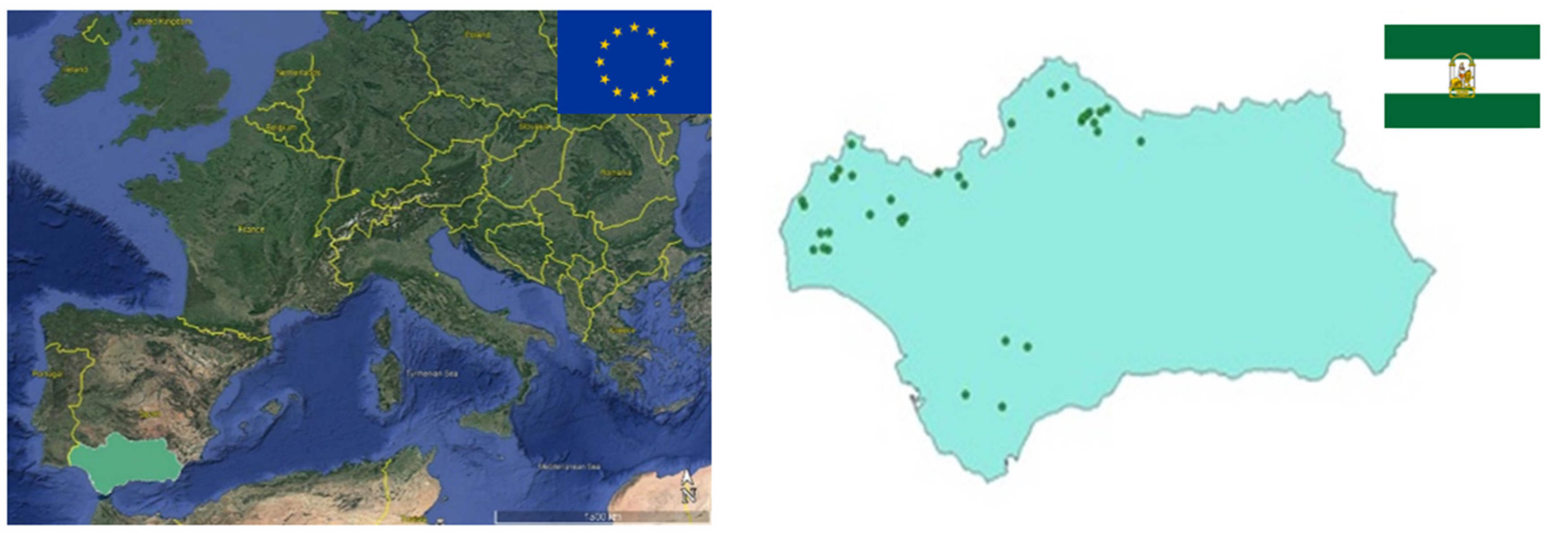
2.1. Study Area

The study area is located in the dehesa zones of southern Spain. Specifically, 32 dehesa farms were selected (represented by the green dots in Figure 1).

They are part of the demonstration areas included within the framework of the LIFE+ bioDehesa project LIFE 11 BIO/ES/000726 [34]. These farms have common elements (trees, copses, regenerated trees, shrubs, pastures, water areas, fauna ...), but there are differences in the quantity, density and species of these elements. The extension of the farms ranges between 150 and 550 ha.

2.2. Image Dataset

The image dataset used in the study came from aerial orthophotographs from PNOA obtained by photogrammetric flights with high resolution digital camera. The image dataset has a spectral resolution of 3 bands (blue, green, red), radiometric resolution of 12 bits per band and spatial resolution of 50 cm.

PNOA images were obtained from the Spanish National Geographic Institute [35] through Web Map Service (WMS) standard [36].

Shapefiles provided by the regional administration [37] were used to metadata the images (for this study, the metadata provided crop and geospatial information).

2.3. Programming Languages

The tool was developed with Python 3.8.5 and MATLAB 2021a (9.10) programming language with two libraries: (i) The Image Analysis Processing toolbox and (ii) openearthtools library from [38]. Python was used for the automatic acquisition of images and identification of the area of interest and MATLAB for the digital processing of the images.

2.4. Procedure

In order to achieve the objective, the development of the tool was carried out with 66 images of approximately 25 ha which were chosen to represent the existing variability in terms of tree density, shrub, pastures and animal species as well as crops and uses of land among the 32 dehesa farms. The development was focused on the correct identification of ecologically significant units (the number of trees, regenerations, copses and water sheets) through image analysis techniques. In addition, the fraction of covered area (FCA) of each of the elements was also obtained. For its implementation, both existing image analysis techniques and new specific developments were combined.

The second step was the validation of the tools, where a further 16 images of 25 ha were used. The real reference of number of individual trees, regenerations, copses and water sheets, was obtained through manual markings with yellow dots, red dots, green areas and blue areas, respectively (Figure 2). The different markings made by hand were counted by means of an algorithm that quantifies the number of each element.

Finally, in order to characterize the farms under study, since the farm is the management unit and the basis for decision-making, the methodology was extended to the entire surface under study (6.377 ha).

2.5. Methodology Flowchart Description

For the sake of clarity, since the main contribution of this paper is the proposal of a methodology, its modules are presented here, which were structured as follows: (i) image acquisition; (ii) standardization: normalization and preprocessing; (iii) segmentation to identify units of interest; (iv) classification using classification techniques based on OBIA rules; and (v) save the results in standardized formats for geographic information systems.

The only parameter required by the tool was an array with the identifiers of the areas under study (local entities (NUTS 4), provinces (NUTS 3), regions (NUTS 2) or countries (NUTS 1)).

The following is a brief description of the modules, their functionalities and the techniques used (see Figure 3). Specific developments (shown in red) carried out to achieve the objectives are shown in the Section 3 since they represent the main contribution of this research.

• Image Acquisition: WMS services [36] were used for the automatic download of the images and shp files [39] to identify areas of interest.
• Standardization. Pre-processing techniques were performed and image homogenization was addressed.
  • Size Standardization: Higher resolution images than 0.5 × 0.5 m (the lowest validated resolution) can be reduced to minimize execution times.
  • Pre-processing: Selection of the color space best suited to object detection, noise reduction and signal smoothing. Specifically: (i) Change to CMYK (Cyan, Magenta, Yellow and Key); (ii) Gaussian noise filtering by linear mean filter (Wiener) and random noise filtering by non-linear median filter (medfilt2) [40]; (iii) illumination correction: adaptive filtering techniques were used to eliminate the lack of illumination [41]; and (iv) contrast adjustment: Histogram equalization techniques were employed [42].
• Segmentation: This is the stage prior to classification, where the objects are identified.
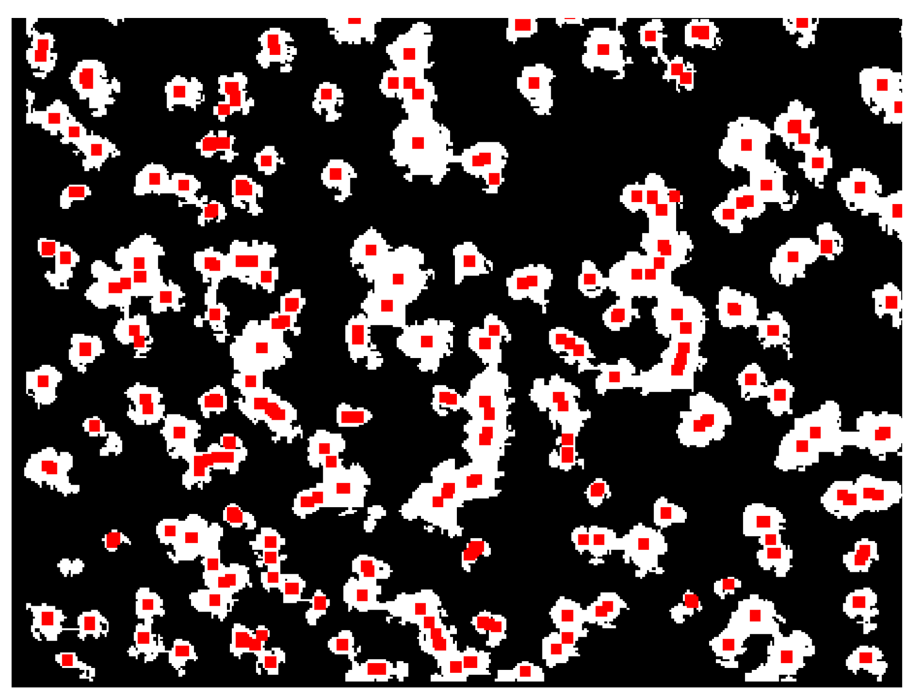
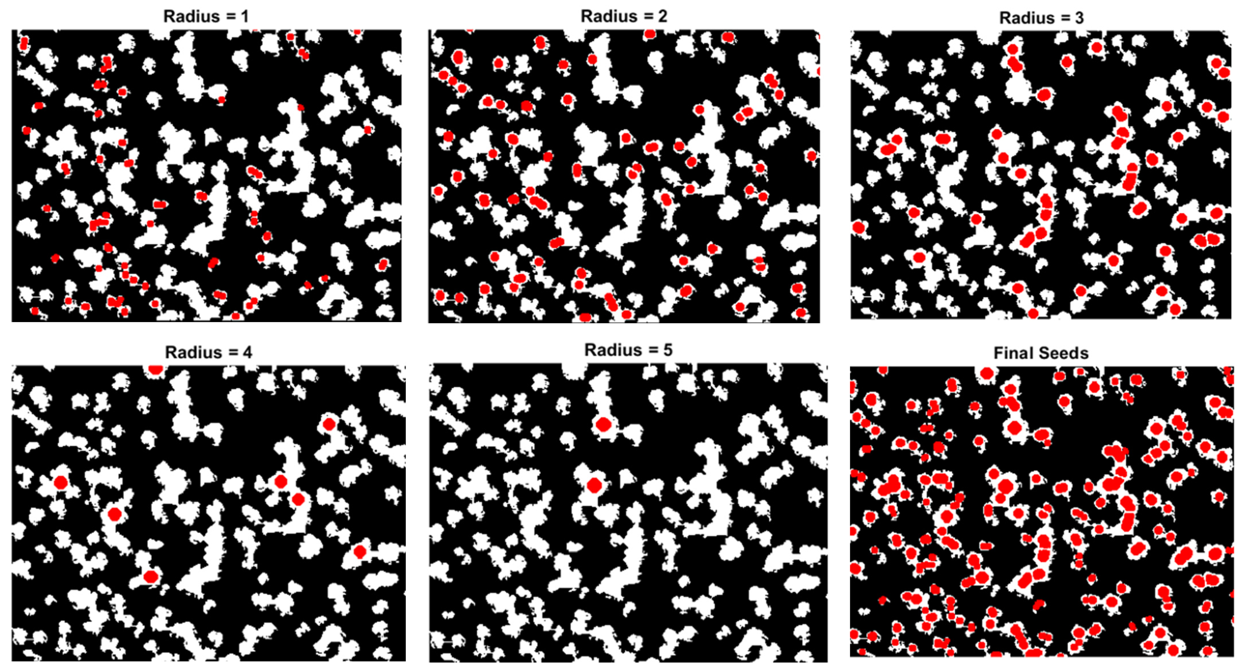
  • Obtaining objects mask: Different segmentation techniques were used for this purpose: (i) Background extraction using the K-means algorithm [43] and seeded region growing method [44,45]; (ii) object detection: Identification of image maxima in non-background areas and growth by region through seeded region growing method [44].
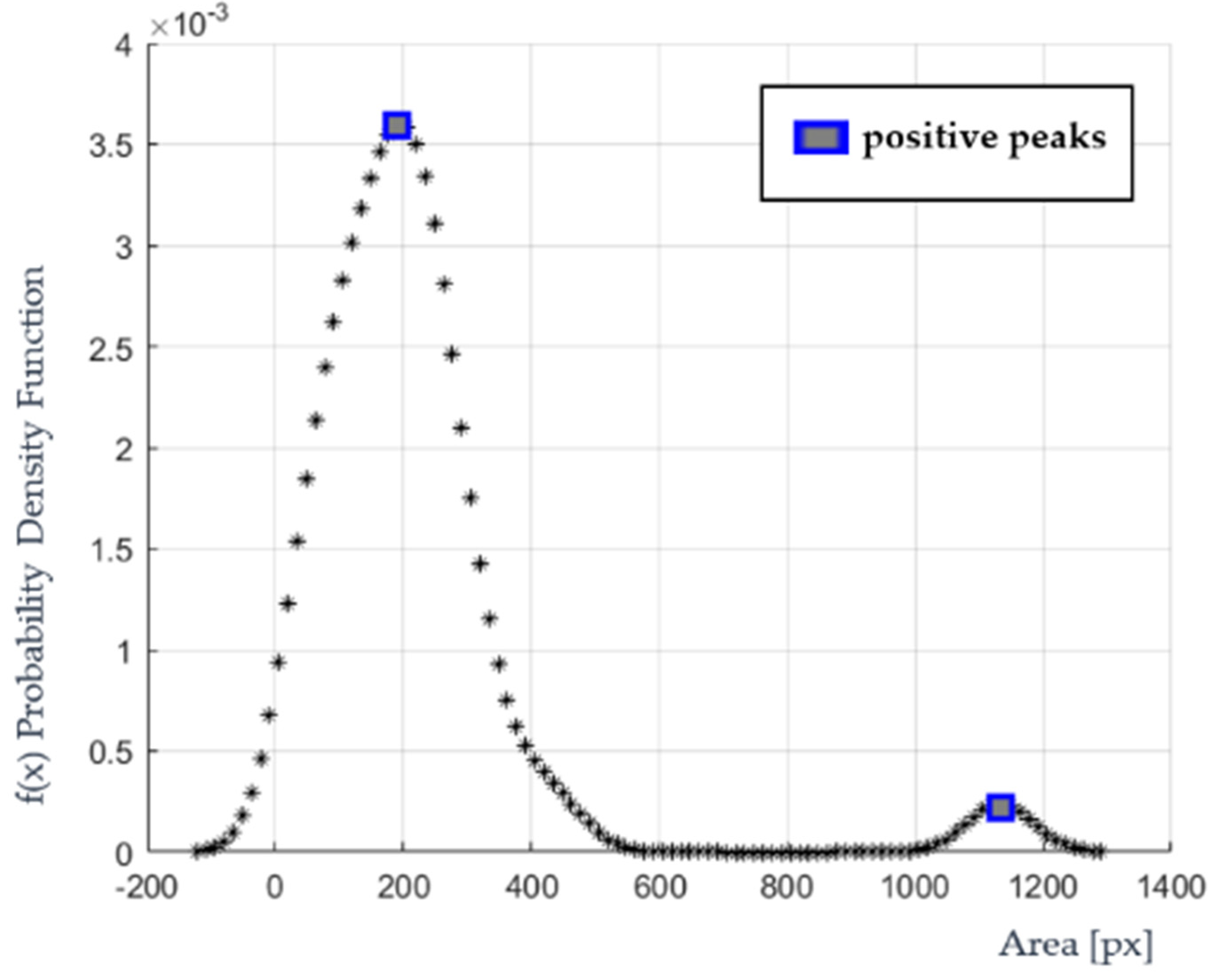
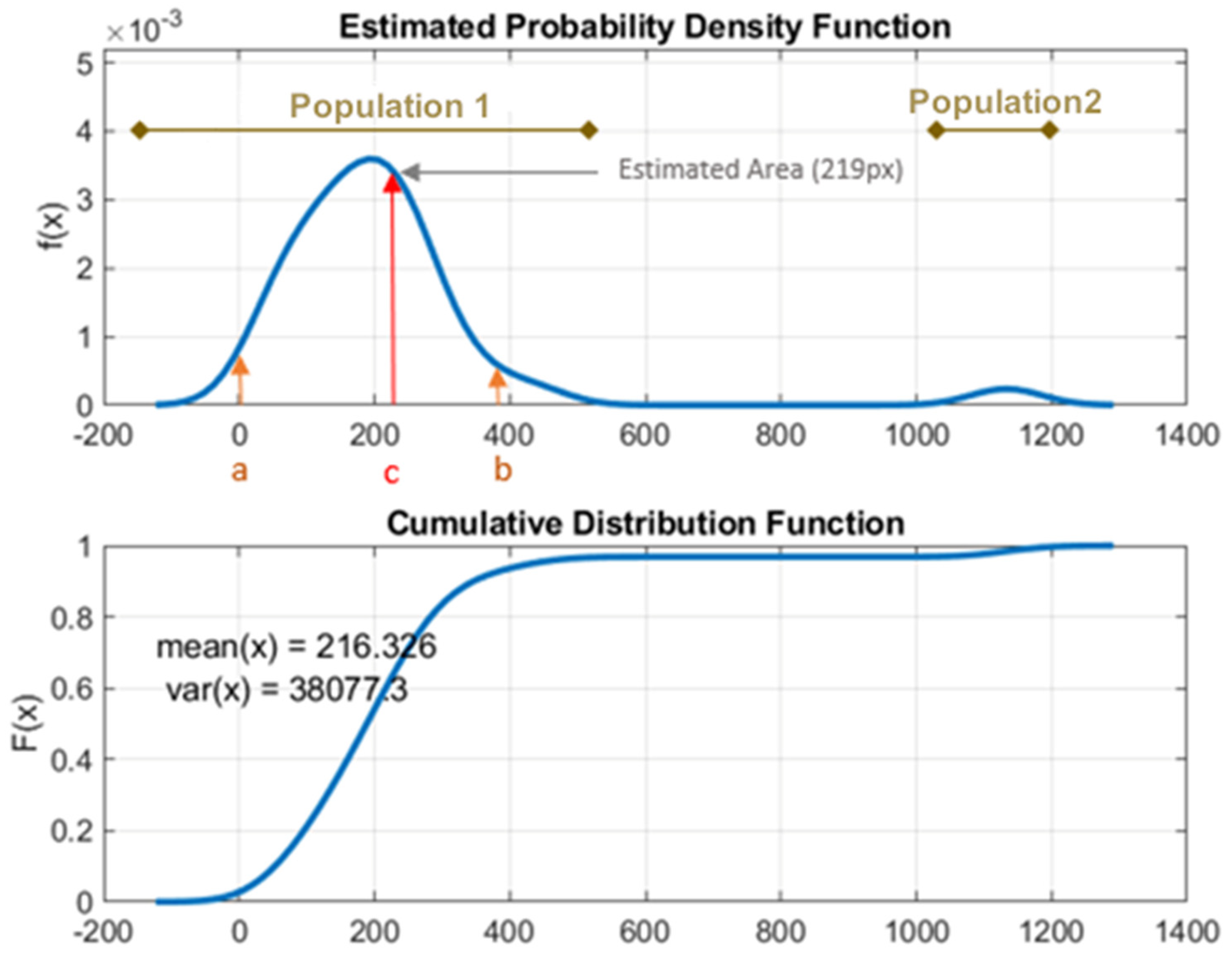
  • Dynamic area estimation: A correct estimation of the area is essential for object division and classification, so a specific development was carried out to optimize the calculation through probability density function (PDF) of the area. This technique is based on the fact that, in systems where groups of elements with differentiated areas coexist, the number of groups, as well as the area of each one, can be determined through the PDF of the area. This development is described on page 7.
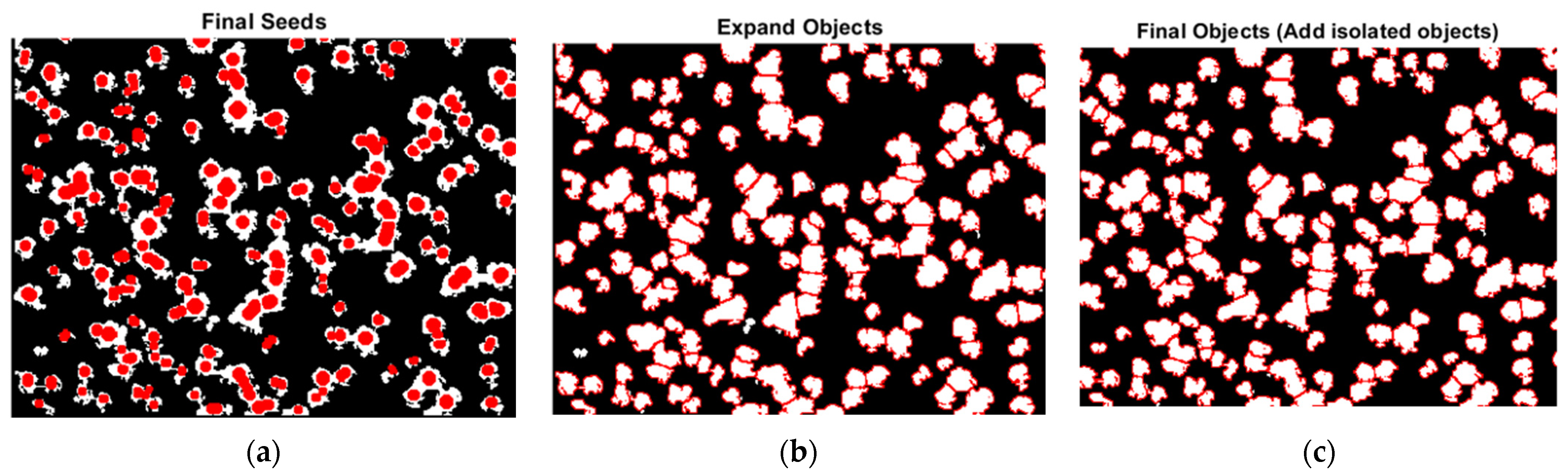
  • Division of objects [46]: two techniques were developed and employed: the first one based on Watershed algorithm [23], the second one based on morphology splitting techniques [26] to split 8-shaped objects. The steps were as follows: (i) Area estimation was carried in previous module, only those elements that were considered clusters will be divided; (ii) the division based on Watershed was performed. This technique was used for the first iteration because it is based on intensity values; (iii) the clusters were re-identified (with the area previously estimated in step (i)); and (iv) the second division was performed, in this case based on morphology.
• Classification: Definitive area estimation through PDF of the area after object division to improve its estimation.
  • Feature spectral and non-spectral extraction [47,48]. For this purpose, patterns of objects containing spectral (colorimetry mean) and non-spectral (size, texture, morphology, solidity, eccentricity and context) information were extracted.
  • A supervised rule-based OBIA classification [47]. This type of classification requires more knowledge of the environment than other self-learning techniques such as those based on Neural Networks or Support Vector Machine.
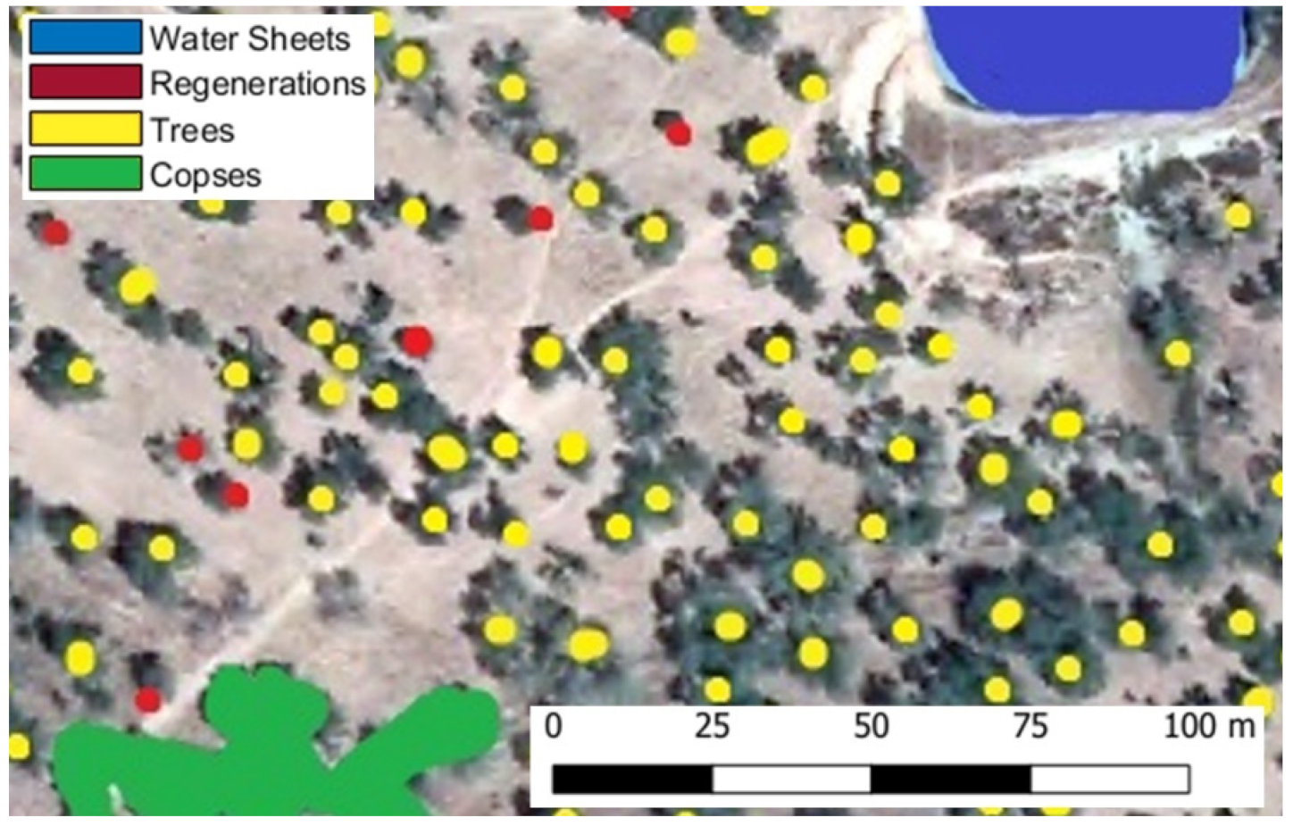
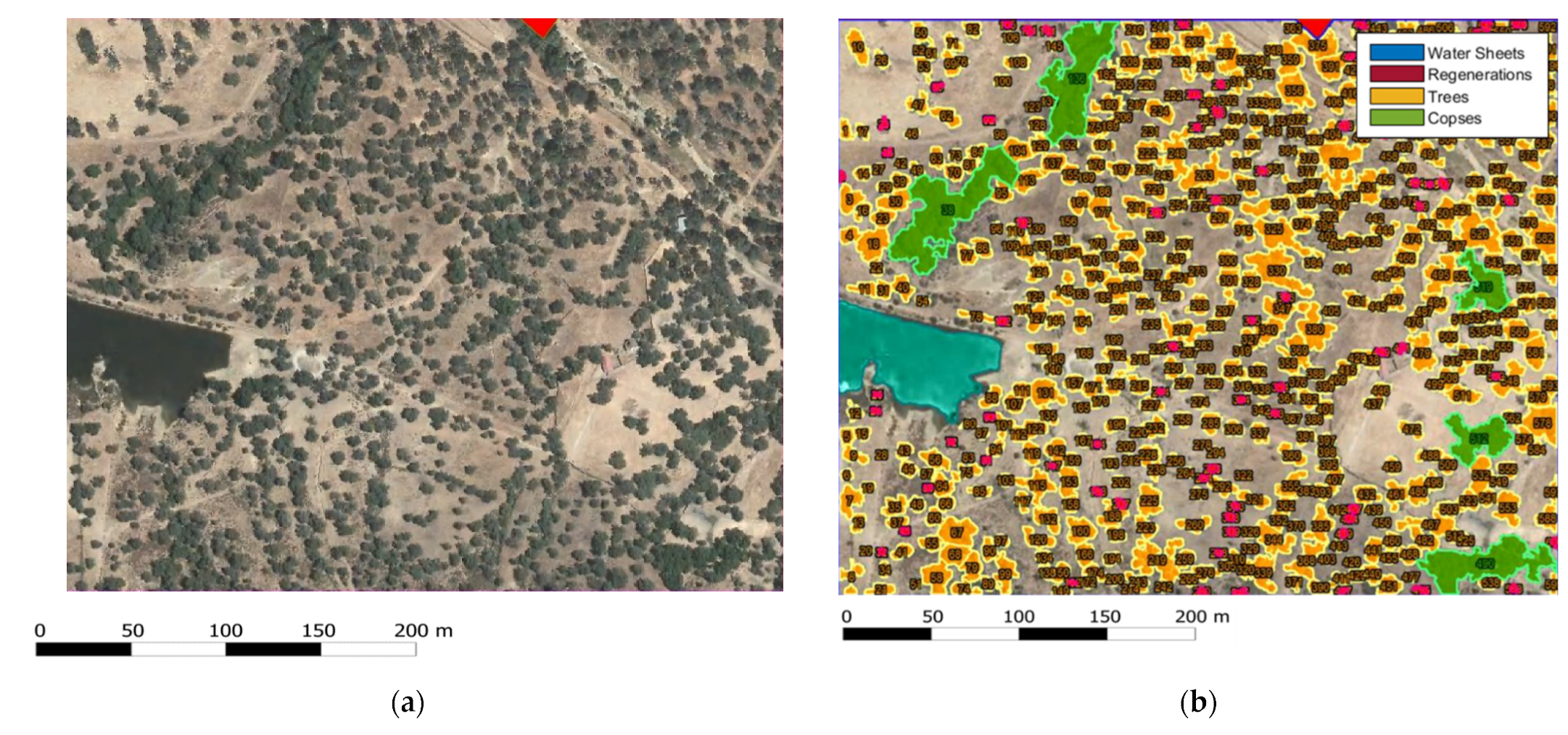
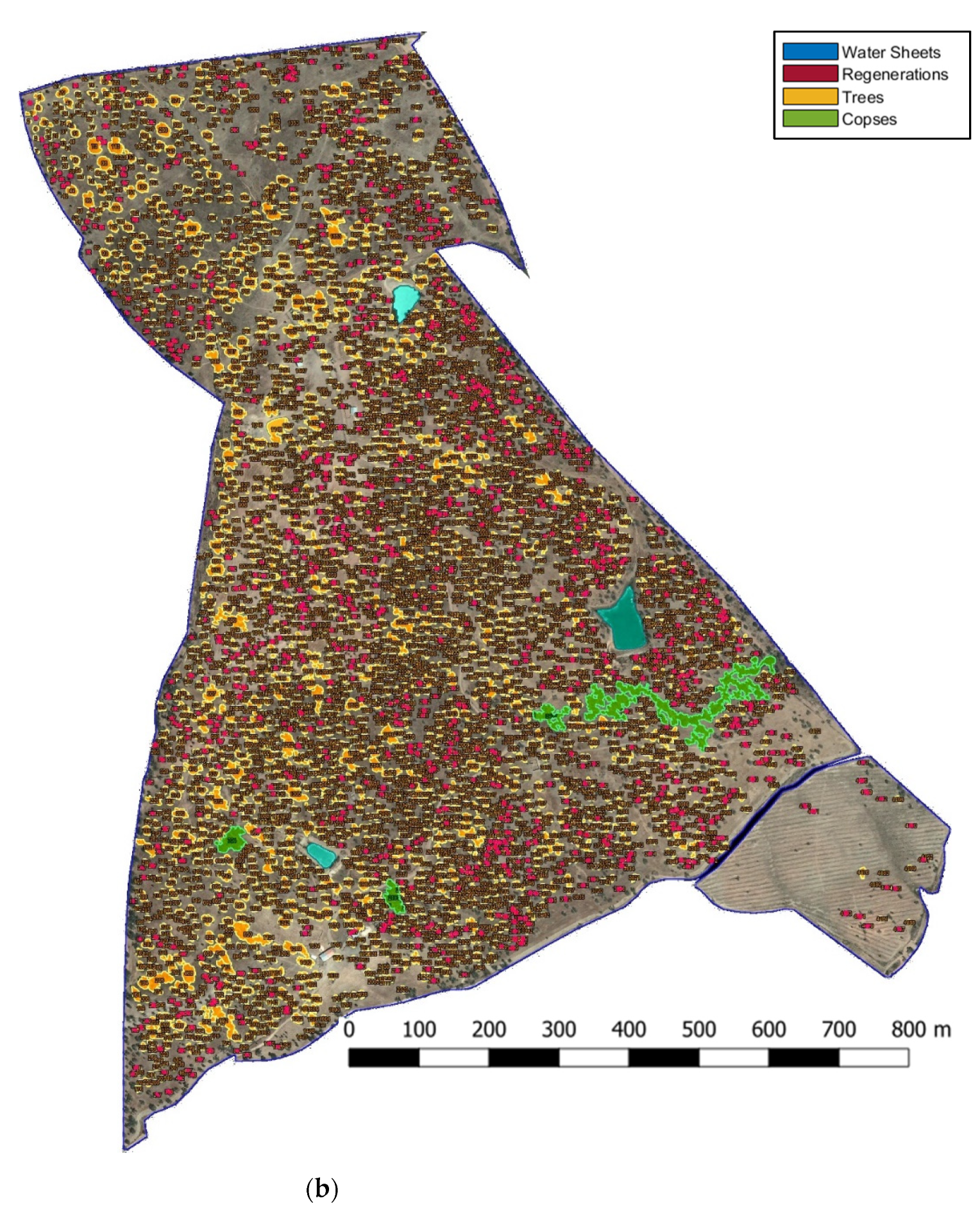
  • Georeferenced raster image where the classified objects were visualized was generated (dark pink for regenerates, yellow for individual trees, green for copses and blue for water sheets). Copses were grouped in terms of proximity.
• Save results: The results were stored in different standardized formats for Geographic Information Systems software or platforms such as Google Earth Engine in order to facilitate further use: (i) Excel File with the relevant image data; (ii) ShapeFile: with relevant object data; and (iii) SQL server database.

3. Results

The main result of this paper is the proposal of a methodology for the automatic identification of the target units as well as the specific developments (shown in red in Figure 3) carried out to achieve this objective. Details are provided so that the specific developments presented here can be reproduced for other data or purposes.

3.1. Specific Developments

3.1.1. Automatic Image Acquisition

This module performs automatic downloading of the image dataset and identifies the ecosystem under study. In order to extend its use to other areas and ecosystems, the module was made configurable, so different characteristics can be set: (i) geographical extension to which it is applied (local entities (NUTS 4), provinces (NUTS 3), regions (NUTS 2) or countries (NUTS 1)); (ii) crop/ecosystem of interest; and (iii) partial download of the images or mosaic of the whole set.

The development was carried out through a Python developed script. TIFF images were downloaded invoking services provided by the National Geographic Institute based on WMS [35] services and AOI was automatically identified through the metadata of the shp files supplied by the regional administration [37], storing the area of interest in a GeoJSON file. This module automates the download/identification and dimensioning of the areas under study of PNOA images through open data sources.

3.1.2. Area Estimation

This method determines the number of existing populations as well as the area of each population by means of the probability density function (PDF) and the cumulative distribution function (CDF) of the area of the elements.

In systems where elements with differentiated areas coexist, the number of populations can be determined through the PDF of the area, by identifying the number of curves. To do so, positive peaks were detected through the segmented peak finder [49], which locates and measures the positive peaks by looking for downward zero-crossings in the first derivative (see Figure 4).

The calculation of the area of each population was obtained by means of cumulative distribution function (CDF), which was used to evaluate probability as area. The cumulative probability density function is the integral of the PDF, and the probability between two values of a continuous random. Equation (1) shows the cumulative distribution function from a to b.

$$P \left(a<x<b\right)={{\displaystyle \int }}_a^{b}f\left(x\right)dx$$

(1)

Based on the above, the area of each population was obtained where the CDF value was 65% of each population (see Figure 5). Considering P (a < x < b) as 90% of that population, the area of the first population was estimated at C point, Equation (2) (65% of P (a < x < b), Equation (3)).

$$Estimated Area=f\left(c\right)$$

(2)

$$P\left(a<x<c\right)={{\displaystyle \int }}_a^{c}f\left(x\right)dx=0.65\times P\left(a<x<b\right)=0.65\times {{\displaystyle \int }}_a^{b}f\left(x\right)d x$$

(3)

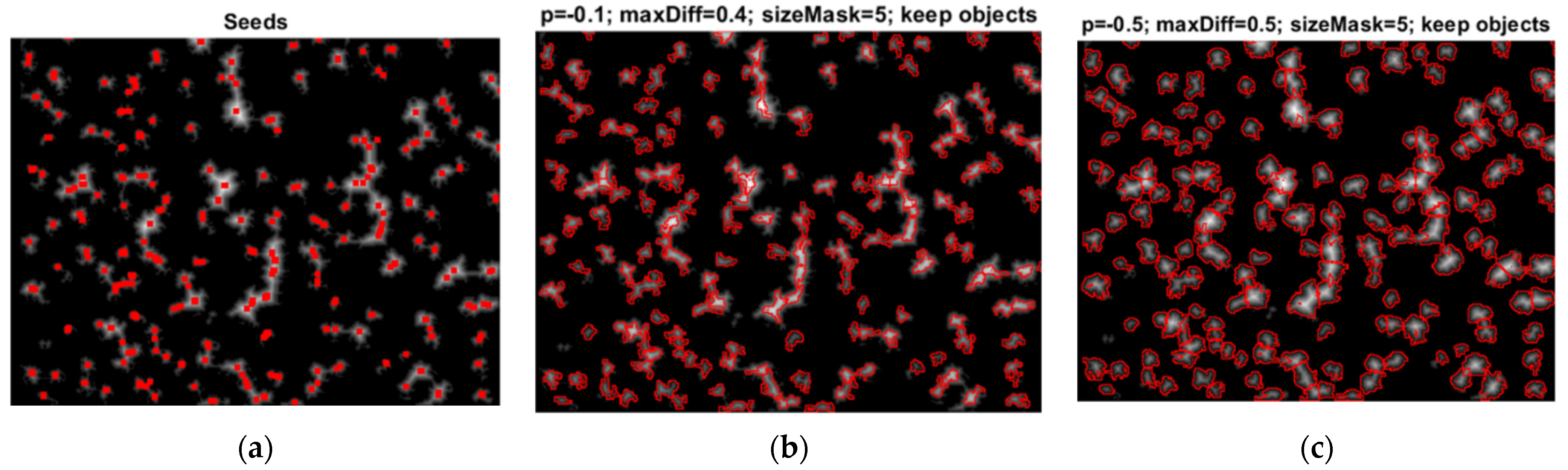
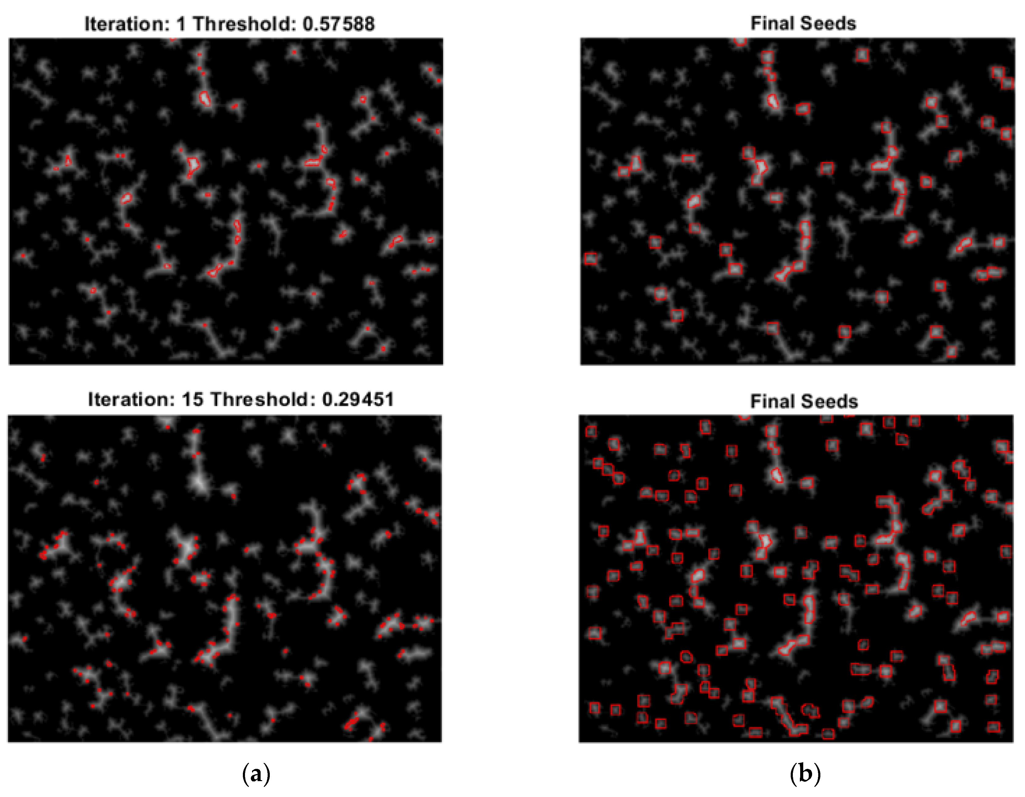
3.1.3. Seeded Region Growing (SRG) Method

We proposed a more parametrizable seeded region growth algorithm [50], which allows a greater adaptation to different methodologies. The parameters used were (i) image: grayscale image; (ii) binaryMask: binary mask limiting object growth; (iii) p: maximum percentage of growth per iteration (p > 0: expand towards a lighter area and p < 0: expand towards a darker area); (iv) iterationMax: number of max pixels you want to explore; (v) sizeMask: size of quadrated mask that is used to calculate the mean values; (vi) mergeObject: 0 if you want to keep objects separated; and (vii) maxDiff: maximum difference between initial pixel value and value of the pixels that will be added to the object (this input must be positive because the evaluation is done over the absolute value of the difference).

The development carried out allows growth towards negative and positive gradients by adding those nearby pixels whose value is less/greater than the mean value of the surrounding area of the object (defined by sizeMask) plus the p value between −1 and 1. It also allows limiting the maximum percentage of object growth by intensity and size (defined by maxDiff and iterationMax), as well as merging or keeping objects separated through mergeObject parameter. Figure 6 shows the execution for different parameters which allows a better adjustment to the needs of the different problems posed.

3.1.4. Object Division

Two methods were developed, one of them based on watershed methodology [51] and the other based on object morphology.

Watershed Method

This method identifies seeds based on maximum intensity and grows in negative gradients. In order to satisfy these requirements, it is necessary to work with the transform of the distance of the mask of objects to be divided (see Figure 7). The growth is conditioned by morphological parameters such as eccentricity, solidity and area.

Firstly, seeds (the brightest objects) were obtained by recursively applying different thresholds (from highest to lowest intensity). In each iteration, new possible seeds were discovered, which can give rise to new seeds or be grouped with the previous ones. The groupings were obtained through agglomerative hierarchical cluster based on minimum distance. The seed search process by iterative method avoids the over-division of the object.

Figure 7a shows the candidates to be seeded in different iterations (1 and 15, respectively, the maximum number of iterations was limited to 15) and Figure 7b shows the final seeds, and it can be observed how in each iteration new seeds appear. Small objects were not identified as seeds because they are isolated objects and splitting is not required.

Subsequently, using seeded region growing (SRG) developed in this study, the seeds were expanded across the negative gradient of the object mask. For the development of our methodology, the parameters used were: sizemask = 5, p = −0.2 (expand towards a darker area) while keeping the objects separated.

As a result, a fully parameterizable wathershed-based methodology was developed, which allows a better adaptation to the problem.

Figure 8 shows an example of results for different parameters: Figure 8a was obtained with minArea = 50, maxArea = 200, MaxEccenrticity = 1, minSolidity = 0 parameters; Figure 8b was obtained with minArea = 150, maxArea = 250, MaxEccenrticity = 0.9, minSolidity = 0.5 parameters. As can be observed, in Figure 8a more optimal results were achieved, because a better approximation of the division of the objects was made. This is due to a better adjustment of the parameters, mainly the object size, which underlines the importance of a correct estimation of the area described on page 7.

Object Division by Morphology

This method was based on the prior knowledge of shape of the objects to be divided (round objects) as well as morphological operations of erosion and dilatation. It divides objects of a binary mask and defined radius. The steps are shown below.

Firstly, seeds were identified by means of erosion techniques and grouped by agglomerative hierarchical cluster based on minima distance (defined by radius). Figure 9 shows the seeds marked in red obtained through morphological operations.

Next, a first morphology-based growth was performed, where the growth constraint of each object is given by its size (larger objects experience higher growth). To achieve the above, the minimum distance from the seed to background was calculated for each object, which constrains it growth. This allows all the seeds to be at an equal distance from the background.

As shown in Figure 10, smaller objects only grow with radius 1 while bigger objects experience a growth of radius 5. This controlled growth allows small objects not to invade the area of large objects in the following phases. Lastly, final seeds are expanded by the initial binary mask and isolated objects are added (Figure 11).

3.1.5. OBIA Classification

Patterns of objects containing spectral (colorimetry mean) and non-spectral (size, texture, morphology, solidity, eccentricity and context) information were extracted for subsequent OBIA-based classification.

• Feature extraction: Spectral and non-spectral attribute extraction

  (a)

  Spectral attributes based on colorimetry of the RGB image (Green Layer) and CMYK (Cyan Layer) color model.

  (b)

  Non-spectral attributes:

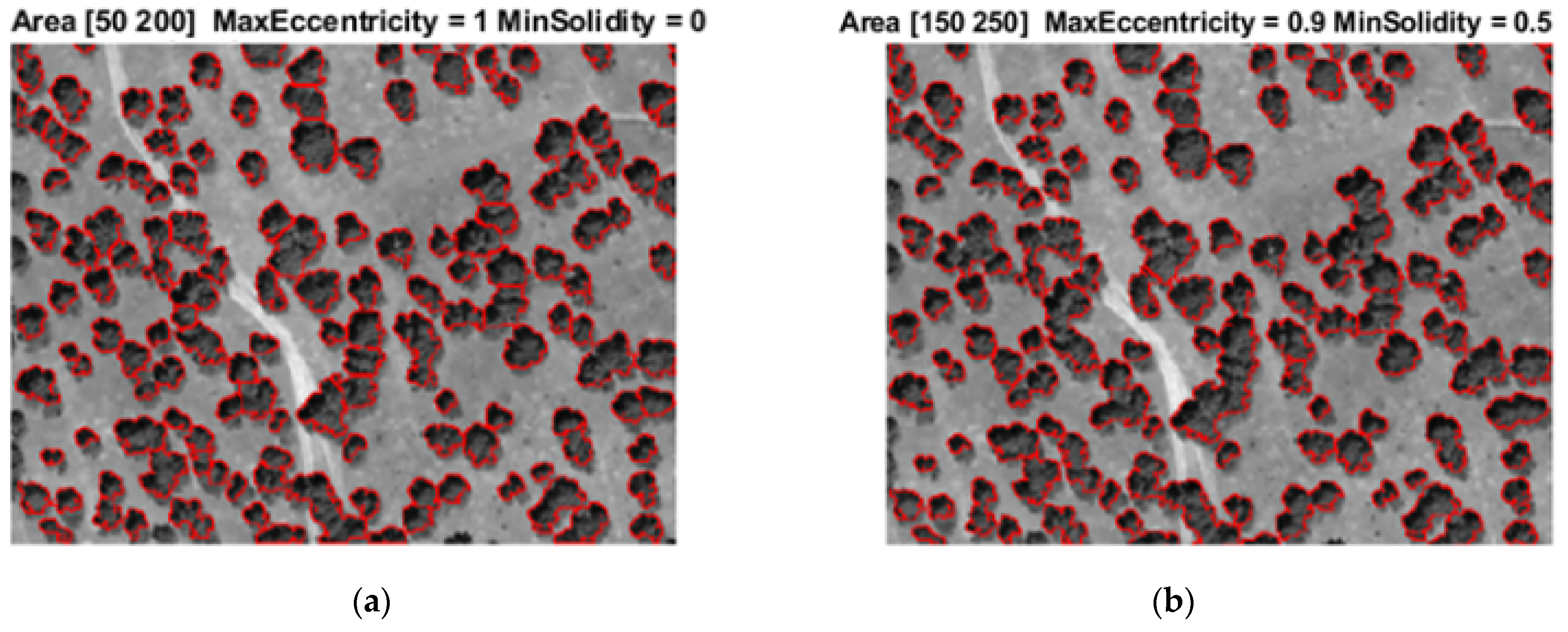
  • Eccentricity (Ecc): parameter that determines the degree of deviation of a conical section with respect to a circumference (0 for circumferences, tends to 1 for very longitudinal elements).
  • Robustness (R): the fraction of area of the region compared to its convex hull. The convex hull is what you would get if you wrapped a rubber band around the region. So, the robustness is the fraction of the actual area of the region, being high for the elements of interest.
  • Texture obtained through STD filters (T_SDT): allows us to differentiate between water sheets and trees, since this attribute is much lower in water sheets.
  • Area (Area): key factor to differentiate between regenerates, independent tree units and copses.

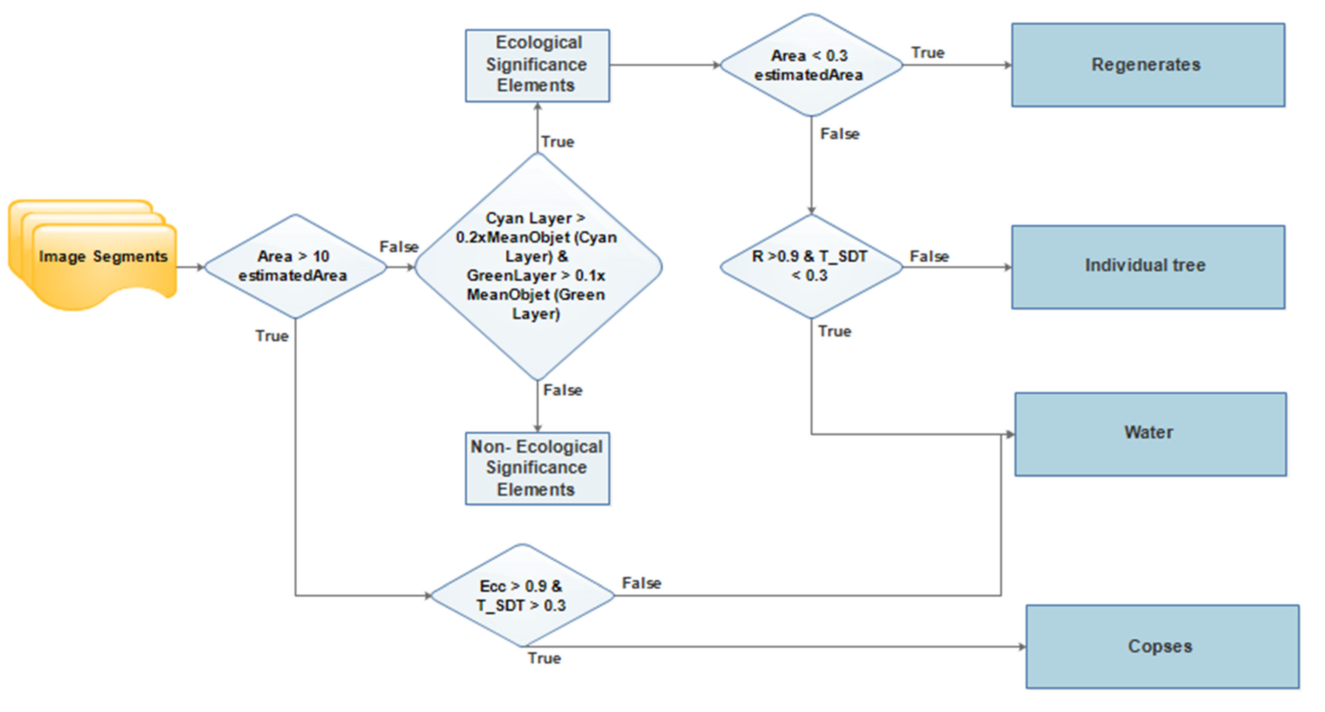
• Rule-based OBIA classification through the spectral and non-spectral attributes (see Figure 12) The classification was carried out using a supervised method, which requires prior knowledge of the elements. Based on this knowledge and the tests carried out during development, the values of the different thresholds were adjusted. The thresholds related to the area were compared with the estimated area in each image, so it is a dynamic threshold.

With regard to the rest of the features that make up the classification, we took into account those that allow us to clearly distinguish between the different elements. Specifically, the STD makes it possible to distinguish between water and vegetation (regenerated, trees and copses), since water has a much lower STD than vegetation. As far as vegetation is concerned, Robustness is quite high for trees and low for copses, while Eccentricity has high values for copses and low values for trees.

Color-based spectral features allowed false positives, such as architectural elements, to be ruled out.

3.2. Tool Validation

An additional set of 16 images was used to validate the tool. Figure 13 shows an example of the result of the tool for one image used for this purpose.

Table 1. Real and calculated values and relative errors of the items under study for 16 images used for the tool validation.

Image ID	Ecological Unit	Real Value	Calculated Value	Relative Error	Image ID	Ecological Unit	Real Value	Calculated Value	Relative Error
1	Trees	952	961	0.9%	9	Trees	982	1003	2.1%
	Regenerations	47	41	12.7%		Regenerations	72	80	11.11%
	Copses	0	0	0%		Copses	1	1	0%
	Water Sheets	1	1	0%		Water Sheets	1	1	0%
2	Trees	755	834	10.4%	10	Trees	716	685	4.4%
	Regenerations	84	85	1.1%		Regenerations	56	61	8.9%
	Copses	3	4	33.3%		Copses	0	0	0%
	Water Sheets	0	0	0%		Water Sheets	1	1	0%
3	Trees	551	534	3.0%	11	Trees	482	510	5.82%
	Regenerations	131	152	7.6%		Regenerations	51	58	13.7%
	Copses	3	3	0%		Copses	10	9	10%
	Water Sheets	0	0	0%		Water Sheets	0	0	0%
4	Trees	49	49	0%	12	Trees	664	658	0.9%
	Regenerations	2	2	0%		Regenerations	34	38	11.7%
	Copses	0	0	0%		Copses	1	1	0%
	Water Sheets	0	0	0%		Water Sheets	0	0	0%
5	Trees	122	125	2.4%	13	Trees	419	449	7.1%
	Regenerations	1	1	0%		Regenerations	13	15	15.38%
	Copses	1	1	0%		Copses	1	1	0%
	Water Sheets	2	2	0%		Water Sheets	1	1	0%
6	Trees	890	776	13.08%	14	Trees	729	737	10%
	Regenerations	81	95	17.28%		Regenerations	191	233	21.9%
	Copses	1	1	0		Copses	3	3	0%
	Water Sheets	0	0	0		Water Sheets	1	1	0%
7	Trees	732	625	14.61%	15	Trees	438	398	9.1%
	Regenerations	65	70	7.6%		Regenerations	15	20	33.33%
	Copses	2	2	0%		Copses	2	2	0%
	Water Sheets	1	1	0%		Water Sheets	1	1	0%
8	Trees	972	912	6.17%	16	Trees	924	899	2.7%
	Regenerations	98	104	6.1%		Regenerations	14	19	35.7%
	Copses	2	2	0%		Copses	0	0	0%
	Water Sheets	1	1	0%		Water Sheets	1	1	0%

shows a summary of the real values and those calculated by the tool when processing the images, as well as the relative errors for each of the elements to be identified for the 16 images used for validation.

In order to study the goodness of fit of the data, a correlation analysis was carried out between the real and the calculated value for each of the target units. The quality of the fit was measured through the coefficient of determination (R-squared). The R-squared values obtained were between 0.97 and 0.99, indicating that the model is capable of explaining 97% of the variability observed in the response variable. The p-values were between 4.29 × 10⁻¹² and 7.13 × 10⁻¹⁰⁹ (far below 0.05) showing that there was evidence that the variance explained by the model is higher than that expected at random.

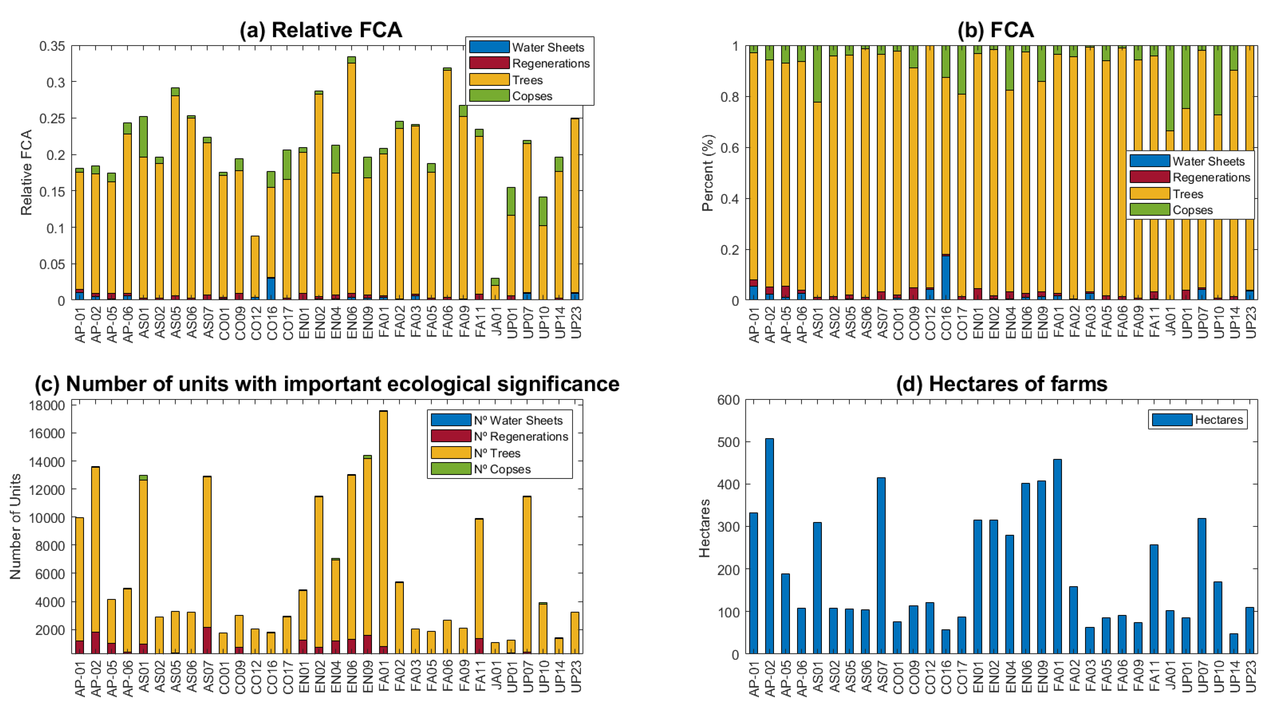
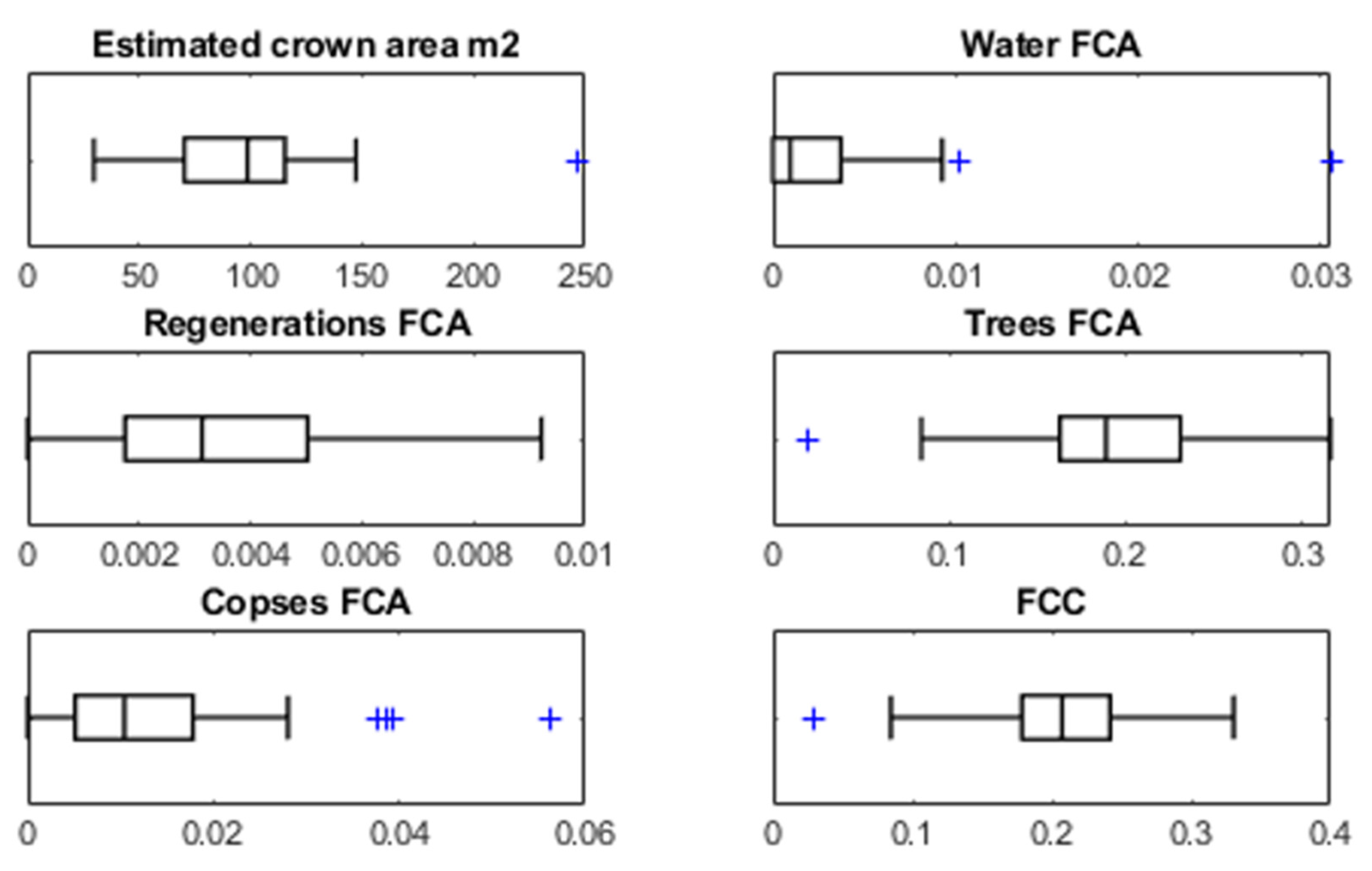
3.3. Extension of the Study

In order to test the scalability and usefulness of the tool developed to characterize management units in real situations, such as complete farms, the tool was applied to the entire area of 32 farms (6377 ha). Figure 14 shows the result of one farm under study.

The characterization of the 32 farms under study through the methodology allowed obtaining relevant attributes such as the number of elements and the FCA of each unit of interest (see Figure 15). The FCA is especially useful for monitoring water sheets and copses, since, although they are few units, they can have relevance within the farm, as is the case in farm CO16. Regarding the number of elements, it is considered important to have a traceability of the number of regenerates or trees. We also extracted generic information such as estimated crown area (estimated using the function developed for this purpose), FCA of each target unit (water sheets, regenerations, tree and copses) as well as the Fraction of Canopy Cover FCC (regeneration FCA + tree FCA + copses FCA) (see Figure 16)

4. Discussion

This work was aimed at developing a methodology to generate automated agroforestry inventories for large area analysis. To do so, a tool was developed with which a stable solution was achieved for the automatic and precise identification of ecological units in dehesa territories. This represents a valuable contribution to the development of tools for landscape characterization and monitoring in a complex agroforestry system, which have become crucial for its sustainability. The results of this work are in line with the results presented in [52], where a methodology for landscape sampling, mapping and characterization of a complex agroforestry system in sub-Saharan Africa was provided. Their results showed the compositional, configurational and functional heterogeneity found in the study area with a satisfactory accuracy of 85.12%. The approach proposed in our study allowed to effectively characterize peculiarities of the dehesa by providing knowledge of its topological distribution, which helps the conservation of its biodiversity, thus saving the complexity of image processing in these types of territories due to the great variety of ecological elements [13,14,15].

Our proposal has achieved individualized traceability by providing detailed information (area, morphology, geolocation) for each target unit, allowing us to discern between small trees, trees and copses. This is essential for different purposes: (i) Feeding models to estimate the number of Iberian pigs that can be released per hectare where the importance of automatic detection is highlighted including the correct identification of acorn trees as well as the need to discern shrubs (young acorn trees that are still unproductive or shrubs that are not oaks) [53]; and (ii) monitoring of understorey cover, growth rates and age of oak mortality, due to the fact that studies carried out in [54] provided solid evidence that land-use practices and management intensity modulate responses of holm oak growth to drought. The tool proposed in this study allows including metadata to delve deeper as well as to extend their area of study.

Another point worth underlining is regeneration in the dehesa due to it being a slow and unpredictable process. Tree loss and lack of regeneration have been identified as one of the main problems of dehesa territories [5]. The tool allows one to measure, evaluate and monitor the regeneration capacity of different areas, which makes it possible to obtain key patterns in the recovery of ecosystems.

More specifically, this work has demonstrated its capacity for the identification and counting of the tree canopy. This had been addressed by different research and techniques: (i) [55] achieved the detection of 71% of the tree based on terrain elevation models through LiDAR and SfM technique; (ii) [56] were able to delimit 93% of the tree crowns and [18] achieved results with errors between 5.88 and 7.99% in mixed temperate forests with geometric approximations models. Their results are slightly more precise than those presented in this work. However, it should be taken into account that the necessary resources and computational calculations required to apply these techniques are much higher; and (iii) regarding studies focused on obtaining CHM through 2D techniques, with multispectral images (R/G/B/NIR) based on OBIA image analysis techniques [57] obtained an accuracy of 80%, and [17], in their best result, after the evaluation of 10 farms, identified 85% of the palm tree crowns. In the present study, the results (errors between 0.9% and 14.61% in the identification of the tree layer) are similar to those presented using the same techniques with the novelty that other elements were also identified with errors between 0% and 33.3%. In addition, 32 farms were characterized (a total of 6.377 ha) with diversity in tree density and distribution, with the difficulty that this entails, as pointed out by [58].

The methodology covers the automatic acquisition of images and identification of regions of interest through external and open sources for different areas (NUTS 4/NUTS 3/NUTS 2/NUTS 1) and ecosystems, which allows expansion of the study areas both geo-graphically and agronomically (other types of crops/ecosystems). This functionality enables the study of the temporal and spatial variability of agroforestry inventories through automatic updates, making it possible to measure their evolution and compare patterns in different regions. For this purpose, there are tools which allow automatic downloading of satellite images such as ESA SNAP (Sentinel Application Platform) [59], plugin SCP for QGIS [60] or Earth Engine which provide easy web-based access to an extensive catalog of satellite imagery and other geospatial data in an analysis-ready format [61], although its higher resolution (10 × 10 m) is lower than that required for the aim of this study. Moreover, SIGPAC (Geographic Information System of Agriculture Parcels of national government) allows identifying areas and enclosures to view them on a map or on highly detailed aerial photographs but does not enable the automatic download and interpretation of the images.

Regarding image analysis processing, the developments carried out in the study present advances in segmentation and object division techniques. The main improvement compared to existing developments is the flexibility in parameterization, which makes it possible to better adjust to different purposes. As far as segmentation is concerned, the development focused on a widely extended technique, the SGR algorithm [62]. Different approaches were found to address it [63] but none of them completely fitted the needs. Concerning the division of the objects, over-division was observed in the methods provided by MATLAB based on watershed [64] so the development of the two functions was required.

In addition, with a view to extending the methodology to other resolutions, dynamic area estimation was implemented, which calculates the number of populations, the relative percentage and the area of each one of them for a set of provided objects.

One aspect of great importance is the potential to use the synergies between automated procedures to identify and characterize different ecological units in pastoral agroforestry systems from very-high-resolution images such as orthophotos with spatial resolution of 0.5 m or greater, which allow calibrating and optimizing the analyses carried out with lower resolution satellite images, completing the analysis of spectral mixtures.

These specific developments can be reproduced for other data or future study.

5. Conclusions

This study addressed the automatic acquisition, identification, and interpretation of elements with ecological significance in dehesa areas with low-cost techniques, computer vision methods and RGB aerial orthophotographs, allowing the automatic and periodic generation of agroforestry inventories in order to study their evolution. The heterogeneity of this stratum in terms of its distribution and irregular coverage of the territory constituted one of the main difficulties to be solved, but a stable solution was achieved that adds one more tool to the decision support system for the conservation and regeneration of the dehesa.

The results obtained allow the automatic analysis of all the dehesa areas of a complete territory and allow obtaining data that help the management of the areas and the verification of indicators associated with norms and rights to obtain public aid.

The proposal of this paper enables obtaining results in standardized formats of Geographic Information Systems and in high-level platforms such as Google Earth Engine. It is also a source of metadating of the elements of ecological significance automatically identified, as well as an improvement to the development of models for the interpretation of satellite images and their use as decision support systems, an aspect that is suggested as an important line of work for the future.

References

1. Díaz, M.; Pulido, F.J. Bases Ecológicas Preliminares Para la Conservación de los Tipos de Hábitat de Interés Comunitario en España; Ministerio de Medio Ambiente, y Medio Rural y Marino. Secretaría General Técnica. Centro de Publicaciones: Madrid, Spain, 2009; ISBN 978-84-491-0911-9. [Google Scholar]
2. European Habitats Directive. Edición en Lengua Española Legislación, Número de Información. Sumario. Página. 1991, Volume 10. ISSN 0257-7763. Available online: https://eur-lex.europa.eu/legal-content/EN/ALL/?uri=OJ:C:2000:111A:TOC (accessed on 1 February 2022).
3. Porqueddu, C.; Ates, S.; Louhaichi, M.; Kyriazopoulos, A.P.; Moreno, G.; del Pozo, A.; Ovalle, C.; Ewing, M.A.; Nichols, P.G.H. Grasslands in ‘Old World’ and ‘New World’ Mediterranean-Climate Zones: Past Trends, Current Status and Future Research Priorities. Grass Forage Sci. 2016, 71, 1–35. [Google Scholar] [CrossRef]
4. Castle, S.E.; Miller, D.C.; Ordonez, P.J.; Baylis, K.; Hughes, K. The Impacts of Agroforestry Interventions on Agricultural Productivity, Ecosystem Services, and Human Well-Being in Low- and Middle-Income Countries: A Systematic Review. Campbell Syst. Rev. 2021, 17, e1167. [Google Scholar] [CrossRef]
5. Carmona, C.P.; Azcárate, F.M.; Oteros-Rozas, E.; González, J.A.; Peco, B. Assessing the Effects of Seasonal Grazing on Holm Oak Regeneration: Implications for the Conservation of Mediterranean Dehesas. Biol. Conserv. 2013, 159, 240–247. [Google Scholar] [CrossRef] [Green Version]
6. Pulido, F.; McCreary, D.; Cañellas, I.; McClaran, M.; Plieninger, T. Oak Regeneration: Ecological Dynamics and Restoration Techniques; Springer: Dordrecht, The Netherlands, 2013; pp. 123–144. [Google Scholar] [CrossRef]
7. Plieninger, T.; Wilbrand, C. Land Use, Biodiversity Conservation, and Rural Development in the Dehesas of Cuatro Lugares, Spain. Agrofor. Syst. 2001, 51, 23–34. [Google Scholar] [CrossRef]
8. Pulido, F.J.; Díaz, M. Regeneration of a Mediterranean Oak: A Whole-Cycle Approach. Écoscience 2016, 12, 92–102. [Google Scholar] [CrossRef]
9. Pulido, F.J. Biología Reproductiva y Conservación: El Caso de La Regeneración de Bosques Templados y Subtropicales de Robles (Quercus Spp.) Plant Reproductive Biology and Conservation: The Case of Temperate and Subtropical Oak Forest Regeneration. Rev. Chil. Hist. Nat. 2002, 75. [Google Scholar] [CrossRef]
10. Gougeon, F.A.; Leckie, D.G. Forest Information Extraction from High Spatial Resolution Images Using an Individual Tree Crown Approach; Canadian Forest Service Publications: Victoria, BC, Canada, 2003; ISBN 0662332725. [Google Scholar]
11. Peña-Barragán, J.M.; Ngugi, M.K.; Plant, R.E.; Six, J. Object-Based Crop Identification Using Multiple Vegetation Indices, Textural Features and Crop Phenology. Remote Sens. Environ. 2011, 115, 1301–1316. [Google Scholar] [CrossRef]
12. Strasser, T.; Lang, S. Object-Based Class Modelling for Multi-Scale Riparian Forest Habitat Mapping. Int. J. Appl. Earth Obs. Geoinf. 2015, 37, 29–37. [Google Scholar] [CrossRef]
13. Raab, C.; Riesch, F.; Tonn, B.; Barrett, B.; Meißner, M.; Balkenhol, N.; Isselstein, J. Target-Oriented Habitat and Wildlife Management: Estimating Forage Quantity and Quality of Semi-Natural Grasslands with Sentinel-1 and Sentinel-2 Data. Remote Sens. Ecol. Conserv. 2020, 6, 381–398. [Google Scholar] [CrossRef]
14. Ramoelo, A.; Cho, M.A. Explaining Leaf Nitrogen Distribution in a Semi-Arid Environment Predicted on Sentinel-2 Imagery Using a Field Spectroscopy Derived Modelss. Remote Sens. 2018, 10, 269. [Google Scholar] [CrossRef] [Green Version]
15. Starks, P.J.; Zhao, D.; Phillips, W.A.; Coleman, S.W. Development of Canopy Reflectance Algorithms for Real-Time Prediction of Bermudagrass Pasture Biomass and Nutritive Values. Crop Sci. 2006, 46, 927–934. [Google Scholar] [CrossRef] [Green Version]
16. Fernández-Habas, J.; García Moreno, A.M.; Hidalgo-Fernández, M.T.; Leal-Murillo, J.R.; Abellanas Oar, B.; Gómez-Giráldez, P.J.; González-Dugo, M.P.; Fernández-Rebollo, P. Investigating the Potential of Sentinel-2 Configuration to Predict the Quality of Mediterranean Permanent Grasslands in Open Woodlands. Sci. Total Environ. 2021, 791, 148101. [Google Scholar] [CrossRef] [PubMed]
17. Tagle Casapia, X.; Falen, L.; Bartholomeus, H.; Cárdenas, R.; Flores, G.; Herold, M.; Honorio Coronado, E.N.; Baker, T.R. Identifying and Quantifying the Abundance of Economically Important Palms in Tropical Moist Forest Using UAV Imagery. Remote Sens. 2019, 12, 9. [Google Scholar] [CrossRef] [Green Version]
18. Apostol, B.; Petrila, M.; Lorenţ, A.; Ciceu, A.; Gancz, V.; Badea, O. Species Discrimination and Individual Tree Detection for Predicting Main Dendrometric Characteristics in Mixed Temperate Forests by Use of Airborne Laser Scanning and Ultra-High-Resolution Imagery. Sci. Total Environ. 2020, 698, 134074. [Google Scholar] [CrossRef] [PubMed]
19. Panagiotidis, D.; Abdollahnejad, A.; Surový, P.; Chiteculo, V. Determining Tree Height and Crown Diameter from High-Resolution UAV Imagery. Int. J. Remote Sens. 2017, 38, 2392–2410. [Google Scholar] [CrossRef]
20. Pouliot, D.; King, D. Approaches for Optimal Automated Individual Tree Crown Detection in Regenerating Coniferous Forests. Can. J. Remote Sens. 2005, 31, 255–267. [Google Scholar] [CrossRef]
21. Culvenor, D.S. TIDA: An Algorithm for the Delineation of Tree Crowns in High Spatial Resolution Remotely Sensed Imagery. Comput. Geosci. 2002, 28, 33–44. [Google Scholar] [CrossRef]
22. Gougeon, F.A.; Leckie, D.G. Forest Regeneration: Individual Tree Crown Detection Techniques for Density and Stocking Assessment. In Proceedings of the Automated Interpretation of High Spatial Resolution Digital Imagery for Forestry; Hill, D.A., Leckie, D.G., Eds.; Canadian Forest Service, Pacific Forestry Centre: Victoria, BC, Canada, 1998; pp. 169–177. [Google Scholar]
23. Uddin, K.; Gilani, H.; Murthy, M.S.R.; Kotru, R.; Qamer, F.M. Forest Condition Monitoring Using Very-High-Resolution Satellite Imagery in a Remote Mountain Watershed in Nepal. Mt. Res. Dev. 2015, 35, 264–277. [Google Scholar] [CrossRef]
24. Goldbergs, G.; Maier, S.; Levick, S.; Edwards, A. Efficiency of Individual Tree Detection Approaches Based on Light-Weight and Low-Cost UAS Imagery in Australian Savannas. Remote Sens. 2018, 10, 161. [Google Scholar] [CrossRef] [Green Version]
25. Bunting, P.; Lucas, R. The Delineation of Tree Crowns in Australian Mixed Species Forests Using Hyperspectral Compact Airborne Spectrographic Imager (CASI) Data. Remote Sens. Environ. 2006, 101, 230–248. [Google Scholar] [CrossRef]
26. Sarabia, R.; Aquino, A.; Ponce, J.M.; López, G.; Andújar, J.M. Automated Identification of Crop Tree Crowns from UAV Multispectral Imagery by Means of Morphological Image Analysis. Remote Sens. 2020, 12, 748. [Google Scholar] [CrossRef] [Green Version]
27. Gougeon, F.A.; Leckie, D.G. The Individual Tree Crown Approach Applied to Ikonos Images of a Coniferous Plantation Area. Photogramm. Eng. Remote Sens. 2006, 72, 1287–1297. [Google Scholar] [CrossRef]
28. Pollock, R.J. The Automatic Recognition of Individual Trees in Aerial Images of Forests Based on a Synthetic Tree. Ph.D. Thesis, University of British Columbia, Vancouver, BC, Canada, 1996. [Google Scholar]
29. Walsworth, N.A.; King, D.J. Image Modelling of Forest Changes Associated with Acid Mine Drainage. Comput. Geosci. 1999, 25, 567–580. [Google Scholar] [CrossRef]
30. Walsworth, N.; King, D. Comparison of Two Tree Apex Delineation Techniques. In Proceedings of the International Forum on Automated Interpretation of High Spatial Resolution Digital Imagery for Forestry; Hill, D.A., Leckie, D.G., Eds.; Canadian Forest Service, Pacific Forestry Centre: Victoria, BC, Canada, 1999; pp. 93–104. [Google Scholar]
31. Korpela, I.; Anttila, P.; Pitkänen, J. The Performance of a Local Maxima Method for Detecting Individual Tree Tops in Aerial Photographs. Int. J. Remote Sens. 2006, 27, 1159–1175. [Google Scholar] [CrossRef]
32. Ke, Y.; Quackenbush, L.J. A Review of Methods for Automatic Individual Tree-Crown Detection and Delineation from Passive Remote Sensing. Int. J. Remote Sens. 2011, 32, 4725–4747. [Google Scholar] [CrossRef]
33. Falk, D.; Campos, A.N. Algoritmo Semiautomático Para El Conteo de Árboles En Plantaciones Forestales Mediante El Uso de Imágenes Aéreas. In Proceedings of the 6o Congreso Argentino de AgroInformática, Universidad de Palermo, Buenos Aires, Argentina, 2–3 September 2014; pp. 186–194. [Google Scholar]
34. Life 11 BIO/ES/000726. Dehesa Ecosystems: Development of Policies and Tools for Biodiversity Conservation and Management. Available online: https://webgate.ec.europa.eu/life/publicWebsite/index.cfm?fuseaction=search.dspPage&n_proj_id=4352 (accessed on 21 September 2021).
35. Instituto Geográfico Nacional. PNOA (Plan Nacional de Ortografía Aérea). Available online: http://www.ign.es/wms-inspire/pnoa-ma (accessed on 1 February 2022).
36. Open Geospatial Consurtium. Web Map Service. Available online: https://www.ogc.org/standards/wms (accessed on 1 February 2022).
37. Junta de Andalucía: Shapefile. Available online: https://www.juntadeandalucia.es/organismos/agriculturaganaderiapescaydesarrollosostenible/servicios/sigpac/visor/paginas/sigpac-descarga-informacion-geografica-shapes-provincias.html (accessed on 1 February 2022).
38. Openearth. Available online: https://www.openearth.nl/ (accessed on 1 February 2022).
39. ESRI Shapefile Technical Description. Available online: https://www.esri.com/content/dam/esrisites/sitecore-archive/Files/Pdfs/library/whitepapers/pdfs/shapefile.pdf (accessed on 1 February 2022).
40. Motwani, M.C.; Gadiya, M.C.; Motwani, R.C.; Harris, F.C. Survey of Image Denoising Techniques. Int. J. Comput. Appl. 2012, 58. Available online: https://www.cse.unr.edu/~fredh/papers/conf/034-asoidt/paper.pdf (accessed on 1 February 2022). [CrossRef]
41. Polesel, A.; Ramponi, G.; Mathews, V.J. Image Enhancement via Adaptive Unsharp Masking. IEEE Trans. Image Processing 2000, 9, 505–510. [Google Scholar] [CrossRef] [PubMed] [Green Version]
42. Stark, J.A. Adaptive Image Contrast Enhancement Using Generalizations of Histogram Equalization. IEEE Trans. Image Processing 2000, 9, 889–896. [Google Scholar] [CrossRef] [Green Version]
43. Krishna, K.; Murty, M.N. Genetic K-Means Algorithm. IEEE Trans. Syst. Man Cybern. Part B Cybern. 1999, 29, 433–439. [Google Scholar] [CrossRef] [Green Version]
44. Skurikhin, A.N.; Garrity, S.R.; McDowell, N.G.; Cai, D.M. Automated Tree Crown Detection and Size Estimation Using Multi-Scale Analysis of High-Resolution Satellite Imagery. Remote Sens. Lett. 2013, 4, 465–474. [Google Scholar] [CrossRef]
45. Wulder, M.; Niemann, K.O.; Goodenough, D.G. Local Maximum Filtering for the Extraction of Tree Locations and Basal Area from High Spatial Resolution Imagery. Remote Sens. Environ. 2000, 73, 103–114. [Google Scholar] [CrossRef]
46. Qiu, L.; Jing, L.; Hu, B.; Li, H.; Tang, Y. A New Individual Tree Crown Delineation Method for High Resolution Multispectral Imagery. Remote Sens. 2020, 12, 585. [Google Scholar] [CrossRef] [Green Version]
47. Zhou, W.; Troy, A. Development of an Object-Based Framework for Classifying and Inventorying Human-Dominated Forest Ecosystems. Int. J. Remote Sens. 2009, 30, 6343–6360. [Google Scholar] [CrossRef]
48. Lu, D.; Weng, Q. A Survey of Image Classification Methods and Techniques for Improving Classification Performance. Int. J. Remote Sens. 2007, 28, 823–870. [Google Scholar] [CrossRef]
49. MathWorks. File Exchange: Segmented Peak Finder FindpeaksSG.m. Available online: https://es.mathworks.com/matlabcentral/fileexchange/60301-segmented-peak-finder-findpeakssg-m (accessed on 1 February 2022).
50. Mary Synthuja Jain Preetha, M.; Padma Suresh, L.; John Bosco, M. Image Segmentation Using Seeded Region Growing. In Proceedings of the 2012 International Conference on Computing, Electronics and Electrical Technologies, ICCEET, Nagercoil, India, 21–22 March 2012; pp. 576–583. [Google Scholar]
51. Kornilov, A.S.; Safonov, I.V. Imaging an Overview of Watershed Algorithm Implementations in Open Source Libraries. J. Imaging 2018, 4, 123. [Google Scholar] [CrossRef] [Green Version]
52. Ndao, B.; Leroux, L.; Gaetano, R.; Diouf, A.A.; Soti, V.; Bégué, A.; Mbow, C.; Sambou, B. Landscape Heterogeneity Analysis Using Geospatial Techniques and a Priori Knowledge in Sahelian Agroforestry Systems of Senegal. Ecol. Indic. 2021, 125, 107481. [Google Scholar] [CrossRef]
53. Ojeda-Magaña, B.; Ruelas, R.; Quintanilla-Domínguez, J.; Gómez-Barba, L.; López de Herrera, J.; Robledo-Hernández, J.G.; Tarquis, A.M. Automatic Identification of the Area Covered by Acorn Trees in the Dehesa (Pastureland) Extremadura of Spain. Comput. Electron. Agric. 2020, 172, 105289. [Google Scholar] [CrossRef]
54. Gazol, A.; Hereş, A.M.; Curiel Yuste, J. Land-Use Practices (Coppices and Dehesas) and Management Intensity Modulate Responses of Holm Oak Growth to Drought. Agric. For. Meteorol. 2021, 297, 108235. [Google Scholar] [CrossRef]
55. Persson, Å.; Holmgren, J.; Soderman, U. Detecting and Measuring Individual Trees Using an Airborne Laser Scanner. Photogramm. Eng. Remote Sens. 2002, 68, 925–932. [Google Scholar]
56. Wack, R.; Schardt, M.; Barrucho, L.; Lohr, U.; Oliveira, T. Forest Inventory for Eucalyptus Plantations Based on Airborne Laserscanner Data. In Proceedings of the ISPRS Workshop 3-D Reconstruction from Airborne Laserscanner and InSAR Data, Dresden, Germany, 8–10 October 2003. [Google Scholar]
57. Johnson, B.A.; Tateishi, R.; Hoan, N.T. A Hybrid Pansharpening Approach and Multiscale Object-Based Image Analysis for Mapping Diseased Pine and Oak Trees. Int. J. Remote Sens. 2013, 34, 6969–6982. [Google Scholar] [CrossRef]
58. Falkowski, M.J.; Smith, A.M.S.; Gessler, P.E.; Hudak, A.T.; Vierling, L.A.; Evans, J.S. The Influence of Conifer Forest Canopy Cover on the Accuracy of Two Individual Tree Measurement Algorithms Using Lidar Data. Can. J. Remote Sens. 2008, 34, S338–S350. [Google Scholar] [CrossRef]
59. Sentinel Application Platform (SNAP). Available online: http://step.esa.int/main/toolboxes/snap/ (accessed on 1 February 2022).
60. QGIS Python Plugins Repository. Available online: https://plugins.qgis.org/plugins/SemiAutomaticClassificationPlugin/ (accessed on 1 February 2022).
61. Gorelick, N.; Hancher, M.; Dixon, M.; Ilyushchenko, S.; Thau, D.; Moore, R. Google Earth Engine: Planetary-Scale Geospatial Analysis for Everyone. Remote Sens. Environ. 2017, 202, 18–27. [Google Scholar] [CrossRef]
62. Adams, R.; Bischof, L. Correspondence Seeded Region Growing. IEEE Trans. Patfern Anal. Mach. Intell. 1994, 16, 641–647. [Google Scholar] [CrossRef] [Green Version]
63. MathWorks. File Exchange Segmentation by Growing a Region from Seed Point Using Intensity Mean Measure. Available online: https://es.mathworks.com/matlabcentral/fileexchange/19084-region-growing (accessed on 1 February 2022).
64. MathWorks. Watershed. Available online: https://es.mathworks.com/help/images/ref/watershed.html (accessed on 1 February 2022).
Figure 1. Location of the dehesa areas under study.
Forests 13 00581 g001
Figure 2. Example of a real reference of target units through manual marking.
Forests 13 00581 g002
Figure 3. Methodology Flowchart. Specific developments carried out in this study are shown in red.
Forests 13 00581 g003
Figure 4. Calculation of the number of populations through positive peaks.
Forests 13 00581 g004
Figure 5. Example of a probability density function curve of the areas of objects.
Forests 13 00581 g005
Figure 6. Results of the SRG method for different parameterizations: (a) Input image with the seeds; (b) result for the p = −0.1, maxDiff = 0.4, sizeMask = 5 and mergeObject = 0 parameters; (c) result for the p = −0.5, maxDiff 0.5, sizeMask 5 and mergeObject = 0 parameters.
Forests 13 00581 g006
Figure 7. Example of iterative seed search process: (a) Possible seed candidates for different applied thresholds; (b) final seeds set.
Forests 13 00581 g007
Figure 8. Results for watershed method developed for different parametrizations. (a) Results for the minArea = 50, maxArea = 200, MaxEccenrticity = 1, minSolidity = 0 parameters; (b) Results for the minArea = 150, maxArea = 250, MaxEccenrticity = 0.9, minSolidity = 0.5 parameters.
Forests 13 00581 g008
Figure 9. Seeds, marked in red, identified through morphological operations such as erosion and dilatation.
Forests 13 00581 g009
Figure 10. Example of object growth by size for different sizes (radius between 1 and 5) and final seeds. The red circles show the seeds detected in each iteration.
Forests 13 00581 g010
Figure 11. Result of the morphology growth algorithm in different steps: (a) Final seeds; (b) result of expanding the seeds by the object mask; (c) final result by adding isolated elements.
Forests 13 00581 g011
Figure 12. Rule-based OBIA classification.
Forests 13 00581 g012
Figure 13. Example of an image selected for the validation: (a) Input image; (b) image processed by the tool. Dark pink for regenerates, yellow for individual trees, green for copses and blue for water sheets for the 16 images used for validation.
Forests 13 00581 g013
Figure 14. (a) Images input; (b) the images processed by the tools. Dark pink for regenerates, yellow for individual trees, green for copses and blue for water sheets.
Forests 13 00581 g014aForests 13 00581 g014b
Figure 15. Analysis of (a) relative FCA of units of important ecological class per farm; (b) FCA percentage of units of important ecological class per farm; (c) number of units with important ecological significance; (d) hectares per farm.
Forests 13 00581 g015
Figure 16. Descriptive statistics of the estimated crown area, water FCA, regeneration FCA, trees FCA, copses FCA and FCC of the 32 areas under study.
Forests 13 00581 g016