Geomorphic and Climatic Drivers Are Key Determinants of Structural Variability of Mangrove Forests along the Kenyan Coast

Abstract

Mangrove forests occur across a diversity of coastal landforms that influence their structural development and productivity. Preliminary studies in Kenya indicate that mangroves growing in the region north and south of Tana River delta have different structural attributes. We hypothesise a close relationship between mangrove distribution, climate and landform types. Floristic composition of mangroves along the coast of Kenya was characterised and differences illustrated using non-metric multidimensional scaling (nMDS). Other structural properties of mangroves such as tree height, basal area, stand density and standing biomass were also assessed and their differences tested using analysis of variance (ANOVA). A hierarchical cluster analysis was used to compare mangrove species based on structural properties. Additionally, a regression fit model was used to investigate the relationship between mangrove standing biomass and possible drivers of variability. The study revealed significant differences in mangrove tree diameter, tree height, basal area, stand density and standing biomass across the sampled sites. High values of structural complexity were observed in estuarine and deltaic settings with high influence of freshwater input whereas low levels of structural complexity were observed for peri-urban with direct human influence. Our findings suggest that structural variability of mangroves in Kenya is highly influenced by geomorphological and climatic variability along the coast as well as the past and present management regimes of the forest.

1. Introduction

Mangrove forests grow in the intertidal areas of tropical and sub-tropical coasts [1]; occurring across a diversity of landforms such as protected bays, lagoons, estuaries, and small islands. These geomorphic features coupled with climatic and human drivers influence the structure and productivity of mangrove forests. As a result, the structural development of mangroves varies with the diversity of coastal geomorphology, climate and management regimes [1,2,3,4]. On a global scale, solar radiation controls the potential maximum development of a mangrove forest [2] while their distribution is limited by sea surface temperature, atmospheric temperature and precipitation [5].

On a regional scale, mangrove development and occurrence are controlled by geomorphological settings such as topographic expression and composition of landforms; climatic conditions such as temperature and precipitation; and oceanographic factors such as wave, tidal and river influences [6,7,8]. At the local scale, forest structure is a function of the tidal regime which is controlled by the topography of the intertidal area. At this scale, mangroves are classified into different forest types—fringing, riverine, over-wash, basin and dwarf forests [9,10]. There may exist all six types of mangrove forests within the regional boundaries of an environmental setting depending on the local effects of waves, tides and river flow [2].

The environmental factors that support and shape the ecological processes occurring within mangrove ecosystems are the forcing functions of that ecosystem [2]. These factors represent different types of energies such as solar radiation, river flows, tides, land formation and precipitation. The summation of energy sources to a mangrove system such as solar radiation or nutrient loading resulting from river flows minus the energy utilised for maintenance and overcoming stress such as high salinity or drought is the energy signature of that system [2,11]. An increase in the energy signature results in higher rates of energy flow that are evidenced by greater biomass productivity within the mangrove system [2]. This concept of energy signatures to describe mangrove ecosystem structure and function is similar to the concept by Thom [6,12] of using environmental settings to explain mangrove processes from a geomorphological perspective [2]. Thom [6,12] describes five environmental settings where terrigenous sediment inputs are dominant and three settings dominated by the accumulation of carbonate. This geomorphic approach of associating plants with diverse landforms and substrate conditions has been used in mangrove ecology studies across the world to classify different mangrove environmental settings [6,8,12,13,14,15,16]. Recent work by Worthington et al. [16] classifies the settings into deltaic, estuarine, lagoonal, open coast and carbonate settings.

In Kenya, mangroves are a common feature in deltas, protected bays, creeks, river estuaries and lagoons distributed all along the 600 km coastline [17]. Earlier studies on mangrove forests in Kenya have observed that tree height, basal areas and biomass values vary between areas north and south of River Tana delta [18,19,20]. Classifications of environmental settings based on geomorphology and other forcing functions have been used extensively to describe variability in mangrove forest structure across the world [3,10,14,15,16,21,22,23]. However, to our knowledge, only one study in Kenya has attempted its application [18]. Understanding the relationships between environmental settings and ecological functions is important for mangrove management because this ecosystem is often cited as being controlled by factors emanating from the land, sea and air [10,13,15,24].

The current study had two main objectives, (1) to characterise the structure and floristic composition of mangrove forests along the Kenyan coast, and (2) compare the structural variability of mangrove formations along the coast. The results of the study enable comparisons of ecological processes across different mangrove areas in Kenya. They also enhance our understanding of major environmental forcing functions influencing the growth and development of mangrove forests in Kenya. A major limitation of this study was limited geomorphic and oceanographic data for the Kenyan coast.

2. Materials and Methods

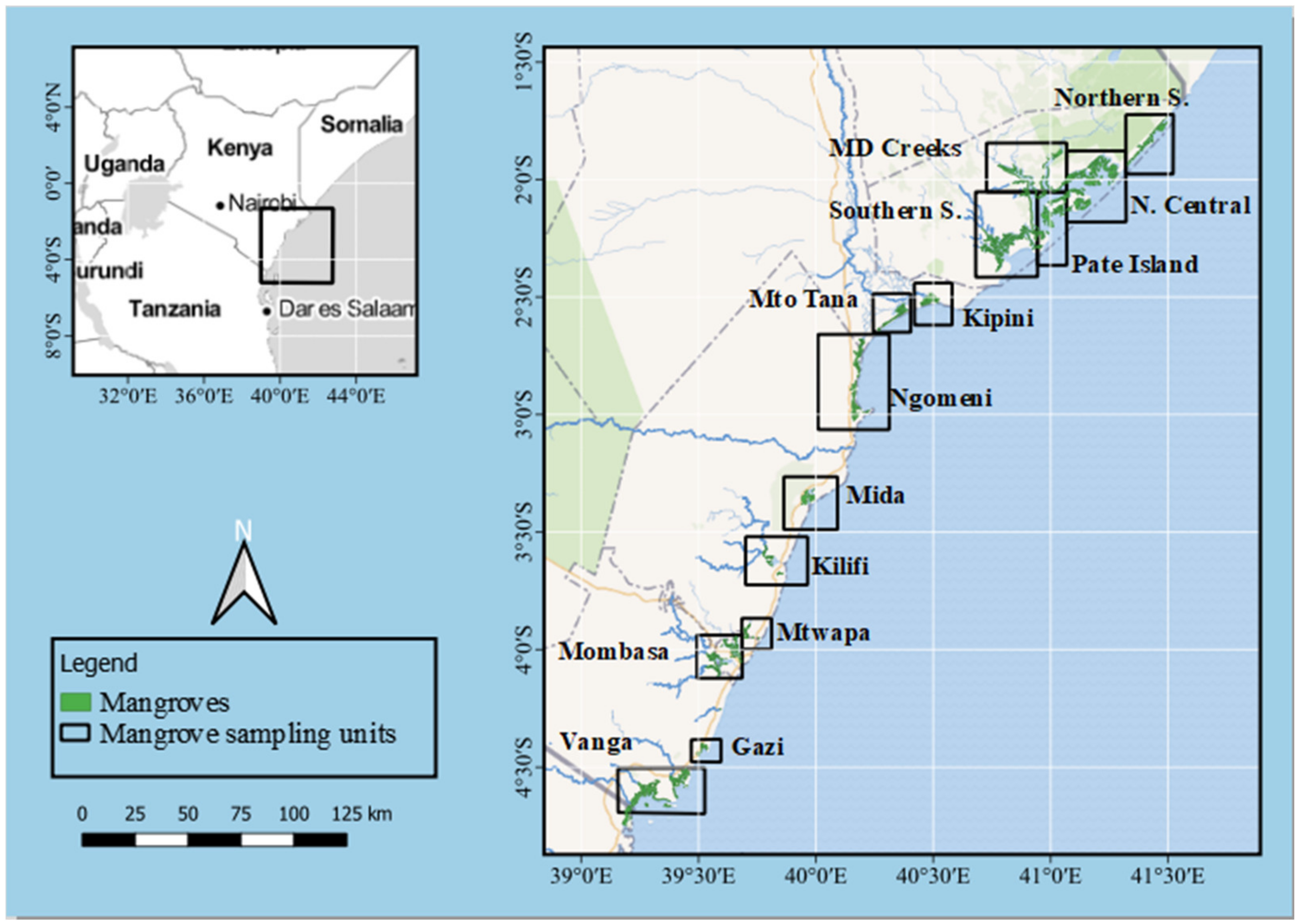
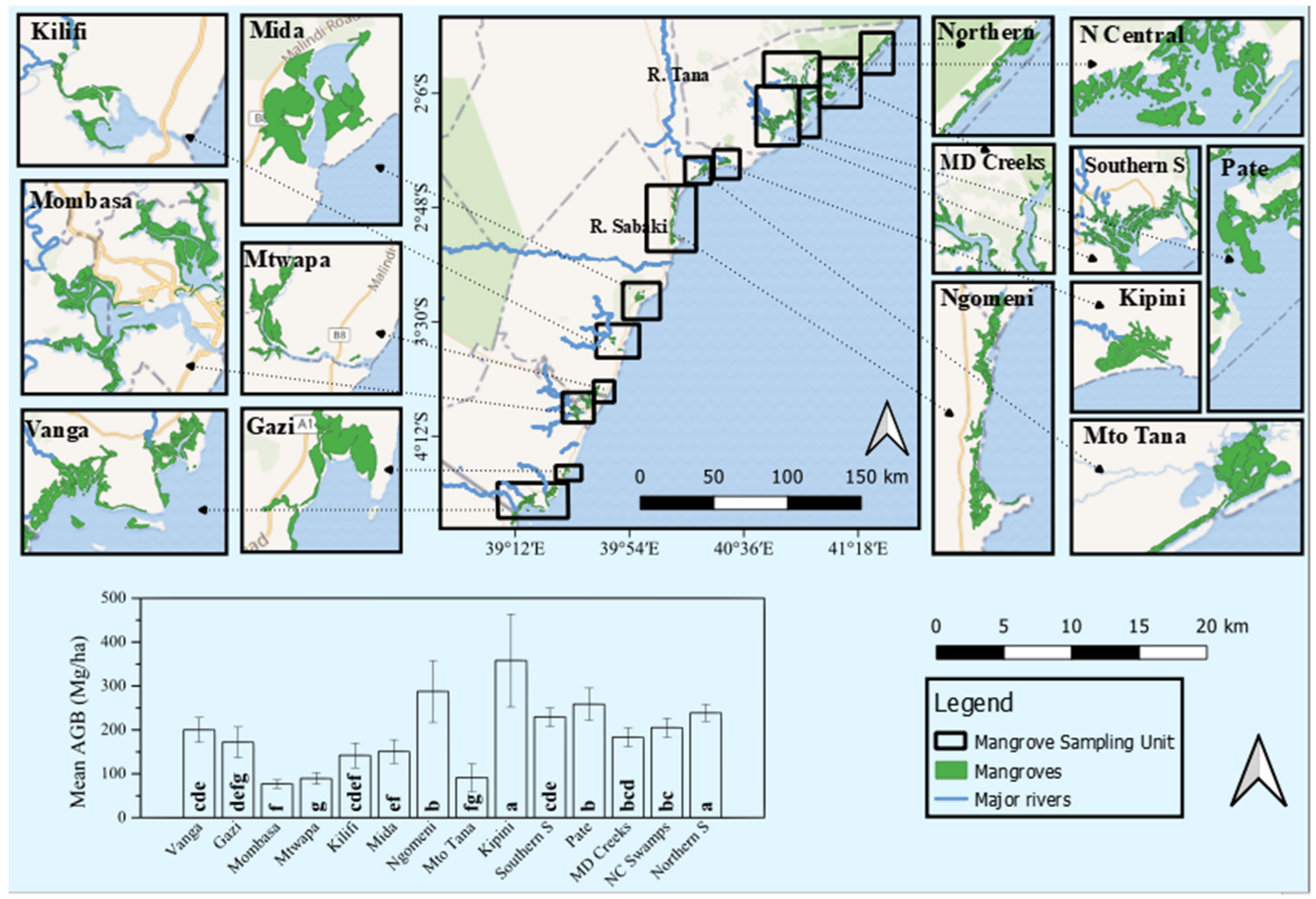
2.1. Description of the Study Area

The Kenyan coastline stretches over 600 km from Vanga at the Kenya–Tanzania border in the south to Ishakani at the Kenya–Somalia border in the north [25] (Figure 1). The coastline straddles five counties—Kwale, Mombasa, Kilifi, Tana River County and Lamu. Distinctive features along the coastline include a semi-continuous fringing reef system, sandy beaches, protected bays, estuaries and tidal creeks that support the natural growth of mangrove forests [17,25,26,27].

All the nine mangrove species described in the Western Indian Ocean (WIO) region [28] occur in Kenya—Rhizophora mucronata, Bruguiera gymnorhiza, Ceriops tagal, Sonneratia alba, Avicennia marina, Lumnitzera racemosa, Xylocarpus granatum, Xylocarpus moluccensis and Heritiera littoralis [17]. These forests occur on reef platforms behind protective outcrops of coral limestone in Lamu; in the estuaries of Tana and Sabaki rivers; behind marine influenced barrier dunes in Ngomeni; in the drowned river valleys of Mombasa, Mtwapa, Kilifi and Mongoni-Dodori; and within the sheltered bays of Vanga and Gazi [17].

The total area of mangroves in Kenya is estimated at 61,271 ha; more than 60% of which occur in Lamu County [17]. Kenya’s National Mangrove Ecosystem Management Plan (2017–2027) identifies 14 mangrove management units in Kenya—hereafter referred to as ‘sites’ (Figure 1). Five of these sites are in Lamu County: Northern Swamps, Northern Central Swamps, Mongoni and Dodori Creek Swamps, Pate Island Swamps, and Southern Swamps. Three of the sites are in Tana River County: Kipini, Mto Tana, and Ngomeni, while three sites are in Kilifi County: Mida, Kilifi, and Mtwapa. Mombasa County is classified as one unit, while Kwale County has two sites: Gazi and the Vanga-Funzi system [17]. This study has maintained this classification scheme for ease of reference and comparisons (Figure 1).

The Vanga and Gazi sites are sheltered bays separated by the Shimoni Peninsula with the Vanga site located at the mouth of River Umba. The Mombasa, Mtwapa and Kilifi sites are peri-urban systems characterised by narrow creeks whose origins are drowned river valleys [29]. The Mida site has a similar morphology to Mombasa, Mtwapa and Kilifi but lacks a discharging river/stream [29]. The Ngomeni, Mto Tana and Kipini sites are located in Ungwana Bay, a wide bay in front of the River Tana Delta that is characterised by fringing dune complexes [29]. The Southern Swamps, Pate Island Swamp, Mongoni-Dodori Creeks, Northern Central Swamps and the Northern Swamps sites are in the coastal lagoons and multiple small islands that define the Lamu Archipelago.

2.1.1. Climate

The coast of Kenya is characterised by a hot and humid tropical climate and experiences a bimodal rainfall pattern influenced by monsoon winds. During March to May, the weather is dominated by the South East Monsoon (SEM) winds leading to heavy rainfall while the North East Monsoon (NEM) winds occur between October and December and are responsible for short rains [25]. The amount of rainfall varies along the coastline due to the inclination of the coast with the northern parts receiving between 500 and 900 mm yr⁻¹ whereas areas south of Malindi receive rainfall ranging between 1000 and 1600 mm yr⁻¹ [26]. Mean daily temperature ranges between 24 and 30 degrees Celsius (ºC) while humidity averages about 80% throughout the year [30].

2.1.2. Oceanography

Kenya’s coast experience semi-diurnal tidal regimes with a maximum tide of 4 m [27]. Major currents influencing the coastal system in Kenya are the East Africa Coastal Current (EACC), the Somali Current (SC) and the Equatorial Counter Current (ECC) [31]. The EACC flows northward throughout the year while the SC is a seasonally reversing current. During the SEM, the SC flows northward as well but reverses during the NEM (Figure 2. The reversed SC meets the EACC somewhere between Malindi and Lamu depending on the strength of the monsoon winds and forms the ECC that flows eastward as an undercurrent [25,31].

2.1.3. Hydrology

Only two perennial rivers drain into the Indian Ocean along the coast of Kenya- Tana and Sabaki rivers. River Tana with a mean annual discharge of about 4000 million m³ branches into a complex deltaic system that opens to the Indian Ocean at Kipini and Mto Tana sites [32]. South of the Tana delta, the Sabaki river drains into the Indian near Malindi town with an annual discharge of about 2000 million m³. The discharge of these two rivers is seasonal and characterised by a bimodal hydrological cycle which corresponds to rainfall patterns [25]. Seasonal rivers draining into the Indian Ocean are Ramisi that drains into the Indian Ocean between the Vanga and Gazi sites, Umba and Mwena that drain into the Vanga site, Mwache that drains in the Mombasa site, and Ndzovuni that drains in the Kilifi site [25,29].

Several freshwater aquifers are distributed along the coastal area of Kenya mainly within the sedimentary terrains. The largest aquifer system stretches from the north eastern parts of the country in Marsabit and terminates in Lamu, spanning about 250 km, part of which is the Merti aquifer [33]. Other aquifers are the Tiwi and Msambweni aquifers in the southern parts of the coast that stretch over 80 km along the coastline [33,34,35,36]. These aquifers are considered important in maintaining groundwater seepage into mangrove forests [35] though information on this remains scanty.

2.1.4. Geomorphology

The morphological structure of the coast of Kenya can be divided into three distinct sections. The southern section running from the Kenya–Tanzania border to Gazi is characterised by wide sheltered bays behind a broken chain of coral reef patches. The central section running from north of Gazi to the mouth of the Sabaki river is characterised by a straight fringing coral reef divided into several segments by narrow tidal outlets of branching bays and estuaries and bounded by steep cliffs on the landward side. The northern section running from the mouth of the Sabaki river to the Kenya–Somalia border is characterised by wide open bays in front of the Tana delta and near the mouth of the Sabaki river that are bordered by long beaches and high dune complexes. Reef patches and sheltered lagoons occur between these open bays [29].

2.1.5. Demography

The coastal counties of Kenya have about 3.9 million inhabitants which is about 8.4% of Kenya’s total population [37]. More than 60% of this population resides in Mombasa and Kilifi counties. Kilifi County has the highest population along the coast with about 1.4 million inhabitants. Mombasa county has the highest population density with 5495 persons per km². It is the largest urban centre in the coast with 97 % of the population dwelling within the city. Tana River County has the lowest population density with 8 persons per km² [38]. It is estimated that about 70% of communities living adjacent to mangroves derive their wood requirements from the forest [17].

2.2. Assessment of Vegetation Structure

The structural characteristics of mangroves in the 14 sites were assessed using a systematic random sampling design. Belt transects running perpendicular to the shoreline were randomly established. Plots measuring 20 m by 20 m were systematically established along these transects to capture the variability resulting from the zonation of mangroves. Across all the sites, a total of 372 plots were established representing an overall sampling intensity of 0.3%. Within each plot, all individual mangrove trees with a diameter at breast height (DBH) ≥ 2.5 cm were identified and counted. Data on tree height (m) and stem diameter (cm) were collected following the procedures outlined by Kauffman & Donato [39]. The ecological importance value (IV) of each species was calculated by summing its relative density, relative frequency, and relative dominance. The basal area (m² ha⁻¹) and stand density (trees ha⁻¹) were obtained following formulae outlined by Cintron & Schaeffer-Novelli [40]. The complexity indices (CI) of the study sites were calculated using Equation (1) below:

$$CI=number of species\times basal area\times stand density\times canopy height\times {10}^{-5}$$

(1)

Considering no robust biomass allometric equations have been developed for mangroves in Kenya, we used the generalised equation for estimating mangrove aboveground biomass (AGB) (Mg ha⁻¹) developed by Komiyama et al. [41] (Equation (2)) but used localised species-specific wood density for mangroves in Kenya developed by Gillerot et al. [42].

$$AGB=0.251\rho D^{2.46}$$

(2)

where AGB is above-ground biomass (Mg ha⁻¹), $\rho$ is wood density (g cm⁻³), D is diameter at breast height (cm).

2.3. Factors Affecting Mangrove Structural Variability

To compare the drivers of mangrove variability, mangrove sites were described based on environmental settings, average annual precipitation, population density and river influence. The environmental settings described in this study were modified to suit the various landforms of the Kenyan coast. The following categories were adopted: estuarine coasts are sheltered coasts with one or more rivers flowing into them and with a free connection to the open sea and include the Vanga and Mombasa sites; lagoonal coasts are shallow inland water bodies that are separated from the ocean by a barrier and include the Gazi, Southern Swamps, Pate Island Swamps and Northern Central sites; tidal creek coasts feature a narrow inlet or estuary that is affected by the flow and ebb of ocean tides and include Mtwapa, Kilifi, Mida, Mongoni-Dodori Creek and Mto Tana sites; deltaic coasts are areas of high river influence with sediment accumulating at the mouth of the river and include Ngomeni and Kipini sites; while open coasts are relatively exposed coasts that are only sheltered from the sea by minor reef segments and reef patches such as the Northern Swamps site.

Table 1. Key characteristics of the sampled sites. Southern S denotes Southern swamps, MD Creeks—Mongoni Dodori Creeks, N Central—Northern Central Swamps.

Site	Environmental Setting	Annual Ave. Precipitation (mm)	Population Density Per sq. km.	River Influence *
Vanga	Estuarine Coast	1109	311	Low
Gazi	Lagoonal Coast	1236	115	Low
Mombasa	Estuarine Coast	1050	6964	Moderate
Mtwapa	Tidal Coast	1090	1627	None
Kilifi	Tidal Coast	954	676	Low
Mida	Tidal Coast	930	537	None
Ngomeni	Deltaic Coast	979	676	High
Mto Tana	Tidal Coast	575	22	Moderate
Kipini	Deltaic Coast	947	58	High
Southern S	Lagoonal Coast	960	77	Low
Pate Island	Lagoonal Coast	960	229	None
MD Creeks	Tidal Coast	960	10	None
N Central	Lagoonal Coast	863	136	None
Northern	Open Coast	560	5	None

* River influence is based on the freshwater discharge levels of the rivers present in a site. High represents a discharge greater than 1500 million m³; moderate (100–215 million m³); low (<100 million m³); no influence represents lack of a discharging river.

below summarises key characteristics of the sampled sites. The average annual rainfall data (1995–2015) were accessed from the Kenya Meteorological Department website: http://kmddl.meteo.go.ke:8081/maproom/Climatology/ (accessed on 15 December 2021). The population density was the average population density per square kilometre in the administrative units where the mangrove sites occur sourced from the Kenya National Bureau of Statistics [38]. The influence of the river on the sites was described in an ordinal scale based on the freshwater discharge levels of the rivers draining into the site [27].

2.4. Data Analysis

Graphical presentation of data was used to describe the structure of mangroves in Kenya. Multivariate analyses were performed to examine the differences in species composition across the sites based on species abundance. An analysis of similarities (ANOSIM) using the Bray-Curtis similarity index was performed followed by a pairwise post-hoc test with a Bonferroni correction to examine variability in species composition across the sites. The data matrix consisted of the standardised abundance of each tree species at different size-class categories in each site. A percent similarities analysis (SIMPER) was used to determine which tree species contributed the most to the differences found. These differences were then illustrated using a non-metric multidimensional scaling (nMDS) ordination plot. The nMDS was plotted in two dimensions (2D) using the Bray–Curtis similarity index. We subjected the structural data to normality tests before performing a Box–Cox transformation. A one-way analysis of variance (ANOVA) followed by a post-hoc Tukey pairwise test was performed (p < 0.05) to individually compare DBH, height, basal area and stand density and above-ground biomass across the different sites. A hierarchical cluster analysis (unweighted paired group mean average and squared Euclidian distances) was then performed to determine the degree of similarity of species from the 14 sites based on complexity index, biomass, DBH, and height. A multiple linear regression with a stepwise selection method was used to fit a model describing associations between standing biomass and the possible drivers of variability. The software, OriginPro 9.0, was used to develop the graphical presentations of the structural data while the multivariate analyses were performed using Paleontological Statistics software (PAST 4) and Minitab 18.

3. Results

3.1. Species Composition

Across all the sites, a total of 34,050 individual mangrove trees were sampled. Based on the importance value (IV) index, Rhizophora mucronata was the most important species in 11 out of the 14 sites sampled—Vanga, Gazi, Mombasa, Mtwapa, Kilifi, Ngomeni, Southern Swamps, Pate Island Swamps, Mongoni-Dodori Creeks, Northern Central Swamps and Northern Swamps. Avicennia marina was the most important species in the estuarine area of Ungwana Bay, covering the Mto Tana and Kipini sites (

Table A1. Structural attributes of the various sampled species across the 14 sampled sites. SE is standard error.

Site	Species	Mean DBH (cm)	SE	Mean Height (m)	SE	Basal Area (m2/ha)	IV
Vanga	Avicennia marina	7.71	0.39	4.51	0.18	132.97	64.24
	Bruguiera gymnorhiza	6.33	0.25	5.02	0.12	44.74	49
	Ceriops tagal	4.63	0.07	3.39	0.05	96.47	106.92
	Lumnitzera racemosa	3.4	0.35	1.43	0.07	0.07	1.95
	Rhizophora mucronata	7.63	0.13	6.06	0.07	612.86	187.68
	Sonneratia alba	18.32	0.99	10.36	0.45	129.58	34.04
	Xylocarpus granatum	7.18	0.34	5.01	0.15	30.78	29.75
Gazi	Avicennia marina	16.41	2.06	8.81	0.73	15.81	35.87
	Bruguiera gymnorhiza	7.94	0.46	5.11	0.26	31.54	87.11
	Ceriops tagal	4.22	0.08	2.75	0.05	30.3	130.4
	Rhizophora mucronata	7.6	0.48	6.53	0.33	98.15	145.44
	Sonneratia alba	11.41	1.14	6.28	0.37	22.25	24.04
	Xylocarpus granatum	8.65	0.84	5.24	0.35	30.15	68.05
Mombasa	Avicennia marina	10.55	0.39	5.69	0.13	178.44	78.99
	Bruguiera gymnorhiza	4.36	0.48	3.41	0.22	0.46	2.85
	Ceriops tagal	4.57	0.13	2.79	0.05	66.74	71.64
	Lumnitzera racemosa	7.55	0.25	3.2	0.4	0.22	1.37
	Rhizophora mucronata	4.57	0.05	4.07	0.03	277.84	196.97
	Sonneratia alba	11.85	0.33	7.11	0.13	145.23	45.24
	Xylocarpus granatum	4.68	0.67	3.52	0.51	0.63	2.89
	Xylocarpus moluccensis	6.5	0.5	7.45	0.05	0.17	1.36
Mtwapa	Avicennia marina	11.65	1.37	5.03	0.36	5.15	16.16
	Ceriops tagal	3.73	0.05	2.08	0.03	27.6	98.91
	Rhizophora mucronata	4.42	0.07	3.5	0.03	91.23	236.7
	Xylocarpus granatum	5.74	0.56	4.02	0.17	2.47	14.89
Kilifi	Avicennia marina	9.93	0.5	5.52	0.28	81.14	108.87
	Bruguiera gymnorhiza	4.09	0.32	3.15	0.21	1.28	23.76
	Ceriops tagal	3.77	0.06	2.08	0.04	17.84	81.18
	Rhizophora mucronata	6.49	0.29	4.43	0.12	103.23	157.68
	Sonneratia alba	8.67	0.66	4.89	0.21	16.44	28.5
Mida	Avicennia marina	11.37	0.98	5.61	0.22	13.95	53.86
	Bruguiera gymnorhiza	11.93	1.76	7.08	0.58	6.83	53.61
	Ceriops tagal	4.29	0.08	3.87	0.06	7.34	156.59
	Rhizophora mucronata	7.27	0.25	6.27	0.12	7.87	141.2
Ngomeni	Avicennia marina	11.36	0.78	5.46	0.21	18.45	89.9
	Bruguiera gymnorhiza	12.2	1.13	7.43	0.43	6.15	45.83
	Ceriops tagal	6.07	0.28	4.86	0.13	4.5	116.14
	Rhizophora mucronata	6.99	0.27	6.55	0.11	11.32	150.72
	Sonneratia alba	11.92	0.96	6.64	0.27	13.55	28.5
	Xylocarpus granatum	18.54	1.42	7.81	0.35	12.77	32.07
Mto Tana	Avicennia marina	7.11	0.25	4.28	0.17	50.79	210.19
	Bruguiera gymnorhiza	9.61	1.8	8.09	1.24	2.38	32.86
	Ceriops tagal	4.79	0.17	3.85	0.12	26.19	184.45
	Rhizophora mucronata	7.03	1.42	8	1.27	0.44	15.35
Kipini	Avicennia marina	7.75	0.23	6.61	0.14	105.1	158.12
	Bruguiera gymnorhiza	16.59	2.55	10.59	1.18	26.01	47.35
	Ceriops tagal	3.55	0.19	4.33	0.14	0.5	11.24
	Heritiera littoralis	13.85	0.96	9.11	0.4	151.03	112.99
	Xylocarpus granatum	10.32	1.02	6.96	0.34	44.91	61.21
Southern Swamps	Avicennia marina	6.89	0.31	3.59	0.13	31.48	25.15
	Bruguiera gymnorhiza	8.13	0.53	4.85	0.12	68.44	60.47
	Ceriops tagal	4.76	0.09	3.21	0.04	97.36	100.74
	Rhizophora mucronata	8.02	0.11	5.81	0.04	735.87	234.07
	Sonneratia alba	12.4	0.75	7.69	0.25	42.75	19.56
Pate Island	Avicennia marina	12.64	0.83	10.76	0.35	30.59	35.35
	Bruguiera gymnorhiza	4.89	0.14	7.32	0.09	13.58	50.98
	Ceriops tagal	4.49	0.29	7.21	0.21	2.39	40.23
	Rhizophora mucronata	9.18	0.27	9.99	0.12	190.65	199.72
	Sonneratia alba	16.34	0.8	12.2	0.26	100.24	73.63
	Xylocarpus granatum	14.94	1.2	10.76	0.43	36.32	21.51
Mongoni-Dodori Creek	Avicennia marina	6.4	0.7	7.08	0.36	32.67	40.5
	Bruguiera gymnorhiza	7.17	0.96	8.75	0.4	7.58	43.1
	Ceriops tagal	6.67	0.23	8.91	0.1	56.28	105.9
	Rhizophora mucronata	7.05	0.28	9.7	0.11	107.8	147.33
	Sonneratia alba	14.4	0.59	12	0.22	64.22	49.9
	Xylocarpus granatum	12.7	1.03	11.31	0.36	26.41	32.03
Northern Central Swamps	Avicennia marina	10.35	1.08	9.76	0.26	61.81	24.15
	Bruguiera gymnorhiza	10.65	1.03	12.08	0.3	28.87	33.94
	Ceriops tagal	5.24	0.08	10.03	0.05	106.78	103.71
	Rhizophora mucronata	8.14	0.16	12.52	0.09	467.67	204.26
	Sonneratia alba	15.48	0.75	14.52	0.25	92.95	31.38
Northern Swamps	Avicennia marina	9.64	0.65	4.78	0.17	24.71	19.93
	Bruguiera gymnorhiza	7.73	0.98	5.91	0.47	6.6	15.4
	Ceriops tagal	6.2	0.18	3.75	0.12	35.43	53.12
	Rhizophora mucronata	11.6	0.19	9.09	0.1	653.74	239.98
	Sonneratia alba	14.13	0.49	7.53	0.19	137.1	50.52

). Mangrove forest species composition differed significantly across the sampled sites (ANOSIM R: 0.24, p = 0.001). The pairwise post-hoc test with a Bonferroni correction shows Kipini as being significantly different from all the other sampled sites (

Table A2. Pairwise p value after Bonferroni correction showing the variability in species composition across the 14 sites along the coastline of Kenya as assessed with ANOSIM.

	Vanga	Gazi	Mombasa	Mtwapa	Kilifi	Mida	Ngomeni	Mto Tana	Kipini	Southern Swamps	Pate	Mongoni-Dodori Creeks	Northern Central	Northern Swamps
Vanga		0.0217	0.0845	0.0009	0.0104	0.0011	0.0321	0.0002	0.0001	0.1558	0.2616	0.0902	0.1681	0.014
Gazi	0.0217		0.0008	0.0241	0.009	0.0148	0.1242	0.0007	0.0004	0.0196	0.0517	0.0639	0.0222	0.0004
Mombasa	0.0845	0.0008		0.0007	0.0284	0.0013	0.0004	0.0011	0.0002	0.0314	0.0047	0.0075	0.0482	0.0648
Mtwapa	0.0009	0.0241	0.0007		0.0037	0.062	0.0066	0.0168	0.0002	0.0013	0.0009	0.0076	0.0058	0.0004
Kilifi	0.0104	0.009	0.0284	0.0037		0.0192	0.0765	0.0951	0.0005	0.0203	0.006	0.0589	0.0418	0.0091
Mida	0.0011	0.0148	0.0013	0.062	0.0192		0.0306	0.0999	0.0003	0.0131	0.0004	0.0021	0.0252	0.0005
Ngomeni	0.0321	0.1242	0.0004	0.0066	0.0765	0.0306		0.0263	0.0002	0.0259	0.0088	0.0602	0.0169	0.0008
Mto Tana	0.0002	0.0007	0.0011	0.0168	0.0951	0.0999	0.0263		0.0001	0.001	0.0001	0.0034	0.0013	0.0003
Kipini	0.0001	0.0004	0.0002	0.0002	0.0005	0.0003	0.0002	0.0001		0.0002	0.0001	0.0004	0.0001	0.0003
Southern Swamps	0.1558	0.0196	0.0314	0.0013	0.0203	0.0131	0.0259	0.001	0.0002		0.0448	0.0365	0.4916	0.0334
Pate Island	0.2616	0.0517	0.0047	0.0009	0.006	0.0004	0.0088	0.0001	0.0001	0.0448		0.254	0.049	0.008
Mongoni-Dodori Creeks	0.0902	0.0639	0.0075	0.0076	0.0589	0.0021	0.0602	0.0034	0.0004	0.0365	0.254		0.0709	0.0087
Northern Central	0.1681	0.0222	0.0482	0.0058	0.0418	0.0252	0.0169	0.0013	0.0001	0.4916	0.049	0.0709		0.1647
Northern Swamps	0.014	0.0004	0.0648	0.0004	0.0091	0.0005	0.0008	0.0003	0.0003	0.0334	0.008	0.0087	0.1647

). The ordination plot from the nMDS shows little grouping of sites except Kipini that appears to form a cluster (Figure 3). Based on the SIMPER analysis, Sonneratia alba (20.1% contribution), Ceriops tagal (19.64% contribution) and Avicennia marina (14.18% contribution) contributed more than half (53.87%) of the differences observed across the sites (

Table 2. Average dissimilarities and species contributions to dissimilarity across the 14 sites along the coastline of Kenya as assessed with SIMPER.

Taxon	Av. Dissim	Contrib. %	Cumulative %
Sonneratia alba	4.395	20.05	20.05
Ceriops tagal	4.306	19.64	39.69
Avicennia marina	3.11	14.18	53.87
Bruguiera gymnorhiza	2.978	13.58	67.46
Rhizophora mucronata	2.473	11.28	78.74
Xylocarpus granatum	2.135	9.739	88.48
Heritiera littoralis	1.672	7.628	96.11
Lumnitzera racemosa	0.6135	2.798	98.91
Xylocarpus moluccensis	0.24	1.095	100

).

3.2. Mangrove Structure and Diversity across the Sites

Mangroves in the Northern Swamps of Lamu had the highest mean DBH (10.95 ± 0.16 cm) while those in Mtwapa recorded the lowest DBH values (4.29 ± 0.05 cm) (

Table 3. Structural attributes of mangroves in the 14 sampling sites along the Kenyan coast. Values are reported as mean ± standard error. The grouping information * from the post-hoc Tukey pairwise comparison post-hoc test at 95% confidence level is reported alongside each variable—the means that do not share a letter are significantly different.

Site	DBH (cm)	Group *	Height (m)	Group *	AGB (Mg ha−1)	Group *
Vanga	7.05 ± 0.09	ef	5.21 ± 0.05	f	199.9 ± 28	cde
Gazi	6.28 ± 0.18	g	4.29 ± 0.10	h	171.9 ± 34.7	defg
Mombasa	5.55 ± 0.06	h	4.21 ± 0.03	h	76.77 ± 9.61	f
Mtwapa	4.29 ± 0.05	i	3.06 ± 0.03	i	89.2 ± 13.4	g
Kilifi	6.53 ± 0.18	fg	3.97 ± 0.09	h	141.9 ± 28.3	cdef
Mida	5.89 ± 0.13	gh	4.89 ± 0.06	g	150.7 ± 27	ef
Ngomeni	8.09 ± 0.22	c	6.04 ± 0.08	e	287.6 ± 70.6	b
Mto Tana	5.95 ± 0.15	gh	4.13 ± 0.10	h	91.2 ± 31.4	fg
Kipini	9.53 ± 0.30	b	7.26 ± 0.14	d	358 ± 106	a
Southern Swamps	7.20 ± 0.08	def	5.03 ± 0.03	fg	229.3 ± 21	cde
Pate Island Swamps	9.45 ± 0.21	b	9.71 ± 0.09	b	258.5 ± 36.5	b
Mongoni Dodori Creek	7.80 ± 0.18	cd	9.43 ± 0.08	b	183 ± 21.3	bcd
Northern Central Swamps	7.42 ± 0.11	de	11.54 ± 0.06	a	205.1 ± 21.5	bc
Northern Swamps	10.95 ± 0.16	a	7.92 ± 0.09	c	238.5 ± 19.4	a

). There were significant differences in DBH across the sites [F (13, 34,050) =163.01, p = 0.000]. Generally, the mangroves growing north of the Sabaki River, except those of the Mto Tana site, had relatively high mean DBH values (>7 cm, Table 3). A similar trend was observed with tree height. Northern Central Swamps in Lamu had the tallest trees overall with an average tree height of 11.54 ± 0.06 m while the lowest tree heights were recorded in Mtwapa (3.06 ± 0.03 m). There were significant differences in tree height across the sites [F (13, 34,050) =1827.28, p = 0.000]. The scatterplots of DBH against mangrove tree height suggest a positive, linear relationship between DBH and height across the sites. However, the regression analysis reveals this relationship is relatively weak, particularly in Mombasa and Mtwapa. (Figure 4).

There were significant differences in stand density across the sites [F (13, 358) = 8.68, p = 0.000]. The lowest stand density was recorded for the mangroves of Northern Swamps (1607 ± 129 trees ha⁻¹) while the highest stand density was for the mangroves of Mtwapa (7856 ± 2094 trees ha⁻¹). The pattern of stand density across the sampled sites showed an inverse relationship with mean DBH with the results of the Pearson correlation analysis indicating a negative correlation between stand density and mean DBH (r = −0.688, p = 0.0006,

Table A3. Results from the Pearson correlation analysis of mean DBH (cm), mean height (m), mean basal area (m² ha⁻¹), mean stand density (trees ha⁻¹) mean above-ground biomass (Mg ha⁻¹) and showing the Pearson correlation values and the p-value.

	Mean DBH (cm)	Mean Height (m)	Basal Area (m2 ha−1)	Stand Density (trees ha−1)
Mean Height (m)	0.668
	0.009
Basal Area (m2 ha−1)	0.777	0.504
	0.001	0.066
Stand Density (Trees ha−1)	−0.688	−0.549	−0.307
	0.006	0.042	0.286
Mean AGB (Mg ha−1)	0.814	0.532	0.968	−0.433
	0.000	0.050	0.000	0.122

Cell Contents: Pearson correlation, p-value (in italics).

). The mangrove forest of Kipini had the highest mean basal area (29.78 ± 6.46 m² ha⁻¹) while Mombasa had the lowest basal area (8.70 ± 0.831 m² ha⁻¹). There were significant differences in mean basal area across the sites [F (13, 358) =5.45, p = 0.000].

The mangrove forest of Pate Island Swamps was the most structurally complex (CI = 35.79) while the mangrove forest of Mto Tana had the lowest complexity index (CI = 5.15). Patterns in complexity index along the sites were similar to the pattern observed for mangrove tree height (m) and basal area (m² ha⁻¹). In forest analysis, complexity indices can be used to define if a forest is under stress [43]. The low values of structural complexity, tree DBH (cm), and tree height (m) observed for the mangroves of Mto Tana are a strong indication of stress within the forest. The mangroves of Mombasa had the lowest mean above-ground biomass (AGB) at 76.77 ± 9.61 Mg ha⁻¹ while those in Kipini had the highest standing biomass at 358 ± 106 Mg ha⁻¹ (Figure 5). There were significant differences in AGB across the sites [F (13, 358) =15.36, p = 0.000].

3.3. Multivariate Analysis

Hierarchical cluster analysis using unweighted paired group mean average and squared Euclidian distances on mean AGB (Mg/ha) revealed distinct groupings across the mangrove sites (Figure 6). Kipini has a unique mangrove assemblage with the highest standing biomass observed in the study. Mombasa, Mto Tana and Mtwapa, are also shown to be significantly different from the rest of the sites. These sites have the lowest biomass and complexity index values recorded in the study. Kilifi and Mida sites, both located in Kilifi County in the central region of the coastline are shown to be similar. These sites share some similarities with Northern Central swamps, Vanga, Gazi and Mongoni-Dodori creeks, located in the northern and southern regions of the coastline. Ngomeni, Pate Island Swamps, Southern Swamps and Northern Swamps are also shown to be similar. The multiple linear regression analysis indicated environmental settings and population density best explained the variability in standing biomass. The fit regression model explained 86.74% of the variance in standing biomass.

4. Discussion

This study revealed significant differences in mangrove forest structure along the coast of Kenya. High values of standing biomass and structural complexity were observed in the riverine mangroves of the Tana Delta as well as mangroves found in the protected islands of Lamu Archipelago in the northern parts of the coastline. High values of standing biomass were also observed within the sheltered bays of the southern parts of the coastline. In the central region characterised by drowned river valleys, a fringing coral reef and peri-urban settings, relatively lower levels of standing biomass and structural complexity were observed. These patterns of mangrove structural variability closely follow the patterns of geomorphological variability along the coastline [29].

Mangroves in the northern region of Kenya are influenced by the interplay between run-off from River Tana, hydrodynamics and air–sea interactions [44]. During the south east monsoon (SEM), high levels of sediment and nutrients are deposited from the hinterland into the ocean by River Tana and River [32,45]. Nutrient availability is key in enhancing mangrove growth and productivity [4]. However, it is probably the maintenance of balance between mineral nutrients and substrate salinity that is relevant, rather than the absolute nutrient levels [4]. For instance, the Heriteria littoralis dominated forest of the Kipini site at the mouth of River Tana receives copious amounts of freshwater, sediment and nutrients from the hinterland leading to higher productivity and overall biomass [32,45]. Conversely, the scrub mangroves growing in the Mto Tana site are majorly composed of dwarf trees due to low freshwater and sediment supply. Currently, the River Tana flows directly into an estuary at Kipini rather than in the complex system of channels and distributaries leading to its old mouth at Mto Tana. The little freshwater that still flowed into the old delta through the Kalota brook was blocked through the construction of a multi-purpose community dam in 1988 [29]. This, together with the presence of solar salt works around the area has ultimately limited mangrove growth in the site.

In the sites north of the Tana river (Southern swamps, Pate Island Swamps, Mongoni-Dodori Creek, Northern Central Swamps and Northern Swamps), the northern flowing EACC moves nutrient-rich sediment from the estuaries of the Tana and Sabaki rivers though long-shore transport and is responsible for productivity in the area [44]. These nutrients are later resuspended during the northeast monsoon (NEM) when the north flowing EACC meets the south flowing Somali Current (SC) causing upwelling and nutrient enrichment [44]. The presence of groundwater seepage in the area is another factor that could be driving the productivity of mangroves in the area by providing freshwater into the system [33,34,36]. The management system could also be responsible for the luxuriant growth of mangroves in some parts of Lamu. The Northern Swamps mangroves and some parts of Northern Central Swamps fall under the Kiunga Marine National Reserve (KMNR), where commercial exploitation of mangroves is prohibited [46]. This could explain the high DBH values observed in KMNR.

Compared to the northern parts of the coastline, nutrient levels in Ramisi and Umba river systems in the southern region are relatively low [29]. The differences in the sediment loading, nutrient levels and freshwater input between the river systems of the northern and southern regions explains the different levels of productivity between the northern and southern parts of the coastline of Kenya [29].

In the Vanga area, small, persistent, localised upwelling events occur around the narrow zonal strip that extends between Northern Pemba Island and the mainland, right at the border between Kenya and Tanzania during the NEM. These upwelling events are as a result of the instabilities of the EACC around the chain of islands (Mafia, Unguja and Pemba) and along the continent’s lateral boundary [47]. Halo et al. [47] suggest that these upwelling events occur on-shore throughout the annual cycle evident by the development of near shore negative wind stress curls and consequent positive Ekman vertical velocities during the NEM. The presence of an intermittent stream (Mkurumudji river), ground water aquifers (the Tiwi and Msambweni aquifers) [35], as well as intensive community-based mangrove conservation activities could explain the high structural complexity of mangroves in the Gazi site. The carbon offset project, Mikoko Pamoja in Gazi has played a role in the restoration and protection of mangroves in the area [48].

On the other hand, the mangroves in the central region are influenced by the geomorphology of the area as well as human influences. In this region, the transition of the littoral to the paralic zone is marked by a broken chain of prominent hills of the coastal range. The elevated areas of the coastal range and the Giriama hills lands have protected the littoral zone against strong fluvial erosion and sedimentation. This is evident by the development of a continuous reef complex in the littoral zone of the central region [29]. This coupled with the absence of perennial rivers partly explains the low biomass observed in the mangroves of this region comprising of Mtwapa, Kilifi and Mida. The availability of terrigenous sediments plays a crucial role not only in providing nutrients necessary for mangrove growth but also in providing the necessary accommodation space for mangrove colonisation. For instance, the mangroves of Mtwapa and Kilifi occur in an area characterised by steep cliffs on the margin of the land and the ocean with a narrow tidal zone. Hence, there is limited accommodation space available for mangrove colonisation. The dominance of Ceriops tagal in Mida resulting from past selective logging of desirable Rhizophora mucronata trees [18] could possibly explain the lower values of standing biomass. Ceriops tagal has a relatively lower DBH and mean height compared to the Rhizophora mucronata and Avicennia marina that dominate the rest of the sites (Table A1). The peri-urban mangroves in Mombasa are mainly threatened by human stressors such as overharvesting, habitat conversion, pollution and sedimentation [49].

High values of mangrove standing biomass were observed in estuarine and deltaic sites as well as in sites located in Lamu County (

Table 4. Summary attribute table describing the environmental settings, forcing functions and structural properties of mangroves along the Kenyan coast. (1) denotes the number of species encountered in each site, (2) is basal area (BA) (m² ha⁻¹), (3) is canopy height (m), (4) is stand density (SD) (trees ha⁻¹), (5) is standing/aboveground biomass (AGB) (Mg ha⁻¹), (6) is complexity index (CI). Basal area, canopy height, stand density and standing biomass are reported as mean ± standard error. Southern is Southern swamps, MD Creek is Mongoni Dodori Creek, NC is Northern Central swamps, Northern is Northern swamps.

Site	Environmental Setting	Mangrove Structural Properties
		(1) Species	(2) BA	(3) Height	(4) SD	(5) AGB	(6) CI
Vanga	Estuarine coast	7	19.7 ± 2.2	5.2 ± 0.1	2987 ± 279	199.9 ± 28	21.5
Gazi	Lagoonal Coast	6	20.8 ± 3.6	4.3 ± 0.1	3730 ± 561	171.9 ± 34.7	19.9
Mombasa	Estuarine Coast	8	8.7 ± 0.8	4.2 ± 0.0	2113 ± 154	76.8 ± 9.61	6.2
Mtwapa	Tidal Creek	4	14.1 ± 2.2	3.1 ± 0.0	7856 ± 2094	89.2 ± 13.4	13.5
Kilifi	Tidal Creek	5	15.7 ± 2.3	4.0 ± 0.1	3418 ± 627	141.9 ± 28.3	10.7
Mida	Tidal Creek	4	16.1 ± 1.9	4.9 ± 0.1	4913 ± 826	150.7 ± 27	15.4
Ngomeni	Deltaic coast	6	26.1 ± 5.6	6.0 ± 0.1	3179 ± 554	287.6 ± 70.6	30.0
Mto Tana	Deltaic Coast	4	11.4 ± 2.9	4.1 ± 0.1	2739 ± 749	91.2 ± 31.4	5.2
Kipini	Deltaic Coast	5	29.8 ± 5.9	7.3 ± 0.1	2164 ± 391	358 ± 106	23.4
Southern	Lagoonal Coast	5	21.7 ± 1.5	5.0 ± 0.0	3092 ± 213	229.3 ± 21	16.9
Pate Island	Lagoonal Coast	6	26.7 ± 3.4	9.7 ± 0.1	2302 ± 315	258.5 ± 36.5	35.8
MD Creek	Tidal Creek	6	18.4 ± 1.8	9.4 ± 0.1	2169 ± 296	183 ± 21.3	22.6
NC	Lagoonal Coast	5	19.4 ± 1.4	11.5 ± 0.1	2496 ± 272	205.1 ± 21.5	28.0
Northern	Open Coast	5	22.6 ± 1.5	7.9 ± 0.1	1607 ± 129	238.5 ± 19.4	14.4

* CI is equal to: number of species (1) × basal area (2) × stand density (4) × canopy height (3) × 10^−5.

). Mangroves are facultative halophytes and are more productive in riverine systems with high inputs of freshwater and nutrients [4]. There is evidence of longshore transport of nutrients to the mangroves of Lamu area deposited from the Tana and Sabaki rivers [44]. This demonstrates linkages between mangrove structural properties and geomorphologically defined habitats as described by the concept of environmental settings [8,12,21]. However, relatively lower values of mangrove standing biomass were also recorded for some sites within similar estuarine settings such as Mombasa and Mto Tana. While these areas should have supported high levels of mangrove productivity, the lower biomass values observed could be explained by the presence of human-induced stressors that act to limit mangrove growth and productivity [29,49]. This shows that in addition to the interactions between ecological and geomorphological processes, human influence is also a key factor in driving mangrove forest structure in Kenya. A fitting explanation of mangrove structural variability would have to include the feedback processes resulting from the interactions between the forest and the communities living around them. This includes influences that improve the conservation of mangroves (positive feedback) as well as influence the degradation of the mangrove ecosystem (negative feedback).

Twilley [2,11] explains that the amount of structure that develops in a mangrove system will be determined by the net energy available to the system—the difference between the energy available to the system—solar, chemical (organic matter and nutrient input) and mechanical energy (wind, tides and waves) and the energy required for maintenance or for overcoming stress- hyper salinity, drought, and actual biomass removal through harvesting. All external factors of coastal systems could be evaluated in the form of energy and measured in units of energy such as kilocalories or joules and this could be useful in explaining and predicting patterns of mangrove structural development in Kenya.

5. Conclusions

Mangrove forests in Kenya exhibit differences in floristic composition and structural development that closely follows the patterns of geomorphological and climate variability along the coastline. Effective mangrove management requires an adequate understanding of the forcing functions or potential energies that are present in an area. The management of mangrove ecosystems is most efficient when it prioritises the protection of energy flows and the processes that drive the system. This is because the system retains most of its natural capacity and requires minimal resources and effort to manage [10]. Our findings will be useful to mangrove managers and policy makers to tailor their strategies to ensure mangrove management works with the ecosystem processes in order to achieve more successful outcomes. Further investigation of the physical and chemical parameters within mangrove habitats is required to perform statistical tests and make meaningful comparisons of mangrove ecosystem properties and processes.

References

1. Hogarth, P.J. The Biology of Mangroves and Seagrasses; Oxford University Press: Oxford, UK, 2015; ISBN 0-19-871654-0. [Google Scholar]
2. Twilley, R.R. Properties of Mangrove Ecosystems Related to the Energy Signature of Coastal Environments. In Maximum Power: The Ideas and Applications of H.T. Odum; University Press of Colorado: Boulder, CO, USA, 1995; pp. 43–62. [Google Scholar]
3. Woodroffe, C.D.; Rogers, K.; McKee, K.L.; Lovelock, C.E.; Mendelssohn, I.; Saintilan, N. Mangrove Sedimentation and Response to Relative Sea-Level Rise. Annu. Rev. Mar. Sci. 2016, 8, 243–266. [Google Scholar] [CrossRef] [Green Version]
4. Tomlinson, P.B. The Botany of Mangroves; Cambridge University Press: Cambridge, UK, 2016; ISBN 1-316-79065-7. [Google Scholar]
5. Osland, M.J.; Feher, L.C.; Griffith, K.T.; Cavanaugh, K.C.; Enwright, N.M.; Day, R.H.; Stagg, C.L.; Krauss, K.W.; Howard, R.J.; Grace, J.B.; et al. Climatic Controls on the Global Distribution, Abundance, and Species Richness of Mangrove Forests. Ecol. Monogr. 2017, 87, 341–359. [Google Scholar] [CrossRef] [Green Version]
6. Thom, B. Mangrove Ecology: A Geomorphological Perspective. In Mangrove Ecosystem in Australia: Structure, Function, and Management: Proceedings of the Australian National Mangrove Workshop, Australian Institute of Marine Science, Cape Ferguson, 18–20 April 1979; Australian Institute of Marine Science: Townsville, Australia, 1982; pp. 3–17. [Google Scholar]
7. Snedaker, S.C.; Snedaker, J.G. The Mangrove Ecosystem: Research Methods; UNESCO: London, UK, 1984; ISBN 92-3-102181-8. [Google Scholar]
8. Woodroffe, C. Mangrove Sediments and Geomorphology. In Coastal and Estuarine Studie; American Geophysical Union: Washington, DC, USA, 1993; Volume 7. [Google Scholar]
9. Lugo, A.E.; Snedaker, S.C. The Ecology of Mangroves. Annu. Rev. Ecol. Syst. 1974, 5, 39–64. [Google Scholar] [CrossRef]
10. Schaeffer-Novelli, Y.; Cintrón-Molero, G.; Soares, M.; De-Rosa, T. Brazilian Mangroves. Aquat. Ecosyst. Health Manag. 2000, 3, 561–570. [Google Scholar] [CrossRef]
11. Odum, H.T. An Introduction. In Systems Ecology; Wiley: New York, NY, USA, 1983; ISBN 0471652776 9780471652779. [Google Scholar]
12. Thom, B.G. Coastal Landforms and Geomorphic Processes. Monogr. Oceanogr. Methodol. 1984, 8, 3–17. [Google Scholar]
13. Twilley, R.R.; Rivera-Monroy, V.H. Developing Performance Measures of Mangrove Wetlands Using Simulation Models of Hydrology, Nutrient Biogeochemistry, and Community Dynamics. J. Coast. Res. 2005, 40, 79–93. [Google Scholar]
14. Balke, T.; Friess, D.A. Geomorphic Knowledge for Mangrove Restoration: A Pan-tropical Categorization. Earth Surf. Process. Landf. 2016, 41, 231–239. [Google Scholar] [CrossRef]
15. Twilley, R.R.; Rivera-Monroy, V.H.; Rovai, A.S.; Castañeda-Moya, E.; Davis, S. Mangrove Biogeochemistry at Local to Global Scales Using Ecogeomorphic Approaches. In Coastal Wetlands; Elsevier: Amsterdam, The Netherlands, 2019; pp. 717–785. [Google Scholar]
16. Worthington, T.A.; Zu Ermgassen, P.S.; Friess, D.A.; Krauss, K.W.; Lovelock, C.E.; Thorley, J.; Tingey, R.; Woodroffe, C.D.; Bunting, P.; Cormier, N. A Global Biophysical Typology of Mangroves and Its Relevance for Ecosystem Structure and Deforestation. Sci. Rep. 2020, 10, 1–11. [Google Scholar] [CrossRef]
17. GoK. National Mangrove Ecosystem Management Plan (2017–2027); Kenya Forest Service: Nairobi, Kenya, 2017.
18. Kairo, J.G. Ecology and Restoration of Mangrove Systems in Kenya. Ph.D. Thesis, Vrije Universiteit Brussel, Brussels, Belgium, 2001. [Google Scholar]
19. Ferguson, W. A Land (Scape) Ecological Survey of the Mangrove Resource of Kenya-Draft Report; Forest Department: Nairobi, Kenya, 1993. [Google Scholar]
20. Lang’at, J.K.S. Variability of Mangrove Forests along the Kenyan Coast; Kenya Marine and Fisheries Research Institute: Mombasa, Kenya, 2008. [Google Scholar]
21. Woodroffe, C.D. Pacific Island Mangroves: Distribution and Environmental Settings; University of Hawaii: Honolulu, HI, USA, 1987. [Google Scholar]
22. Woodroffe, C.D. Coasts: Form, Process and Evolution; Cambridge University Press: Cambridge, UK, 2002; ISBN 0-521-01183-3. [Google Scholar]
23. Schaeffer-Novelli, Y.; Cintrón-Molero, G.; Adaime, R.R.; de Camargo, T.M. Variability of Mangrove Ecosystems along the Brazilian Coast. Estuaries 1990, 13, 204–218. [Google Scholar] [CrossRef]
24. Ellison, J.C. Biogeomorphology of Mangroves. In Coastal Wetlands; Elsevier: Amsterdam, The Netherlands, 2019; pp. 687–715. [Google Scholar]
25. Government of Kenya. State of the Coast Report II: Enhancing Integrated Management of Coastal and Marine Resources in Kenya; National Environment Management Authority (NEMA): Nairobi, Kenya, 2017.
26. ASCLME. National Marine Ecosystem Diagnostic Analysis—Kenya; Contribution to the Agulhas and Somali Current Large Marine Ecosystems Project (supported by UNDP with GEF grant financing); UNDP: Nairobi, Kenya, 2012. [Google Scholar]
27. Tychsen, J.; Klinge, H. KenSea. Environmental Sensitivity Atlas for Coastal Area of Kenya. Geological Survey of Denmark and Greenland: Copenhagen, Denmark, 2006. [Google Scholar]
28. Bosire, J.; Mangora, M.M.; Bandeira, S.; Rajkaran, A.; Ratsimbazafy, R.; Appadoo, C.; Kairo, J. Mangroves of the Western Indian Ocean: Status and Management; WIOMSA: Zanzibar, Tanzania, 2015; ISBN 9987-9559-4-0. [Google Scholar]
29. Oosterom, A.P. The Geomorphology of Southeast Kenya. Ph.D. Thesis, Agricultural University, Wageningen, The Netherlands, 1988. [Google Scholar]
30. Okoola, R.E. A Diagnostic Study of the Eastern Africa Monsoon Circulation during the Northern Hemisphere Spring Season. Int. J. Climatol. J. R. Meteorol. Soc. 1999, 19, 143–168. [Google Scholar] [CrossRef]
31. Schott, F.A.; Xie, S.-P.; McCreary, J.P., Jr. Indian Ocean Circulation and Climate Variability. Rev. Geophys. 2009, 47, RG1002. [Google Scholar] [CrossRef]
32. Kitheka, J.U.; Mavuti, K.M. Tana Delta and Sabaki Estuaries of Kenya: Freshwater and Sediment Input, Upstream Threats and Management Challenges. In Estuaries: A Lifeline of Ecosystem Services in the Western Indian Ocean; Springer: Cham, Switzerland, 2016; pp. 89–109. [Google Scholar]
33. Kuria, Z. Groundwater Distribution and Aquifer Characteristics in Kenya. In Developments in Earth Surface Processes; Elsevier: Amsterdam, The Netherlands, 2013; Volume 16, ISBN 0928-2025. pp. 83–107. [Google Scholar]
34. Mwango, F.K.; Muhangú, B.; Juma, C.; Githae, I. Groundwater Resources in Kenya. In Proceedings of the International Workshop on ‘Managing Shared Aquifer Resources in Africa’, Tripoli, Libya, 2–4 June 2002; pp. 93–100. [Google Scholar]
35. Nijsten, G.-J.; Christelis, G.; Villholth, K.G.; Braune, E.; Gaye, C.B. Transboundary Aquifers of Africa: Review of the Current State of Knowledge and Progress towards Sustainable Development and Management. J. Hydrol. Reg. Stud. 2018, 20, 21–34. [Google Scholar] [CrossRef]
36. Oiro, S.; Comte, J.-C. Drivers, Patterns and Velocity of Saltwater Intrusion in a Stressed Aquifer of the East African Coast: Joint Analysis of Groundwater and Geophysical Data in Southern Kenya. J. Afr. Earth Sci. 2019, 149, 334–347. [Google Scholar] [CrossRef] [Green Version]
37. Kenya National Bureau of Statistics. Kenya National Bureau of Statistics. Volume I: Population by County and Sub-County; Kenya National Bureau of Statistics: Nairobi, Kenya, 2019; p. 49.
38. Kenya National Bureau of Statistics. 2019 Kenya Population and Housing Census. Volume II: Distribution of Population by Administrative Units; Kenya National Bureau of Statistics: Nairobi, Kenya, 2019; p. 270.
39. Kauffman, J.B.; Donato, D.C. Protocols for the Measurement, Monitoring and Reporting of Structure, Biomass and Carbon Stocks in Mangrove Forests; CIFOR: Bogor, Indonesia, 2012. [Google Scholar]
40. Cintron, G.; Schaeffer Novelli, Y. Methods for Studying Mangrove Structure. Monogr. Oceanogr. Methodol. 1984, 8, 91–113. [Google Scholar]
41. Komiyama, A.; Poungparn, S.; Kato, S. Common Allometric Equations for Estimating the Tree Weight of Mangroves. J. Trop. Ecol. 2005, 21, 471–477. [Google Scholar] [CrossRef]
42. Gillerot, L.; Vlaminck, E.; De Ryck, D.J.; Mwasaru, D.M.; Beeckman, H.; Koedam, N. Inter-and Intraspecific Variation in Mangrove Carbon Fraction and Wood Specific Gravity in Gazi Bay, Kenya. Ecosphere 2018, 9, e02306. [Google Scholar] [CrossRef]
43. Lewis, R.R., III; Milbrandt, E.C.; Brown, B.; Krauss, K.W.; Rovai, A.S.; Beever, J.W., III; Flynn, L.L. Stress in Mangrove Forests: Early Detection and Preemptive Rehabilitation Are Essential for Future Successful Worldwide Mangrove Forest Management. Mar. Pollut. Bull. 2016, 109, 764–771. [Google Scholar] [CrossRef]
44. Kamau, J.; Ngisiange, N.; Ochola, O.; Kilionzi, J.; Kimeli, A.; Mahongo, S.B.; Onganda, H.; Mitto, C.; Ohowa, B.; Magori, C. Factors Influencing Spatial Patterns in Primary Productivity in Kenyan Territorial Waters. West. Indian Ocean J. Mar. Sci. 2020, 9–18. [Google Scholar] [CrossRef]
45. Kitheka, J.U.; Obiero, M.; Nthenge, P. River Discharge, Sediment Transport and Exchange in the Tana Estuary, Kenya. Estuar. Coast. Shelf Sci. 2005, 63, 455–468. [Google Scholar] [CrossRef]
46. Kairo, J.; Kivyatu, B.; Koedam, N. Application of Remote Sensing and GIS in the Management of Mangrove Forests within and Adjacent to Kiunga Marine Protected Area, Lamu, Kenya. Environ. Dev. Sustain. 2002, 4, 153–166. [Google Scholar] [CrossRef]
47. Halo, I.; Sagero, P.; Manyilizu, M.; Mahongo, S.B. Biophysical Modelling of Coastal Upwelling Variability and Circulation along the Tanzanian and Kenyan Coasts. West. Indian Ocean J. Mar. Sci. 2020, 43–61. [Google Scholar] [CrossRef]
48. Kairo, J.G.; Hamza, A.; Wanjiru, C. Mikoko Pamoja: A Demonstrably Effective Community-Based Blue Carbon Project in Kenya. In A Blue Carbon Primer; CRC Press: Boca Raton, FL, USA, 2018; pp. 341–350. ISBN 0-429-43536-3. [Google Scholar]
49. Mohamed, M.O.S.; Neukermans, G.; Kairo, J.G.; Dahdouh-Guebas, F.; Koedam, N. Mangrove Forests in a Peri-Urban Setting: The Case of Mombasa (Kenya). Wetl. Ecol. Manag. 2009, 17, 243–255. [Google Scholar] [CrossRef] [Green Version]
Figure 1. Map of the study area showing mangrove management units in Kenya. Northern S denotes Northern Swamps; N. Central—Northern Central Swamps; MD Creeks—Mongoni Dodori Creek Swamps; Southern S—Southern Swamps.
Forests 13 00870 g001
Figure 2. Oceanographic currents off the Kenyan coast. The southeast monsoon is shown in red on the right and the northeast monsoon in blue. SC is the Somali Current, EACC is the East African Coastal Current, and SECC is the South Equatorial Counter Current. Source: Tychsen & Klinge [27].
Forests 13 00870 g002
Figure 3. Non-metric multidimensional scaling (nMDS) of sites in two dimensions (2D) based on species abundance. The ellipse shows the 95% confidence interval. The stress level is 0.1304. Southern S is Southern Swamps, MD Creeks is Mongoni-Dodori Creeks, N Central is Northern Central Swamps and Northern S is Northern Swamps.
Forests 13 00870 g003
Figure 4. Height–diameter distribution of mangrove forests in the 14 sampled sites along the coast of Kenya. R2 is the coefficient of determination from regression analysis.
Forests 13 00870 g004
Figure 5. Map of the 14 mangrove sampling sites along the coast of Kenya featuring mean aboveground biomass (Mg/ha) in each site. The error bars are standard error bars, and the letters denote the grouping information from the Tukey Pairwise comparison post-hoc test at 95% confidence level—the means that do not share a letter are significantly different.
Forests 13 00870 g005
Figure 6. A dendrogram from the hierarchical cluster analysis across the 14 sampling sites along the coast of Kenya using unweighted paired group mean average and squared Euclidean pairwise distances.
Forests 13 00870 g006