Article

Spatial Scale Effects of Soil Respiration in Arid Desert Tugai Forest: Responses to Plant Functional Traits and Soil Abiotic Factors

1
College of Ecology and Environment, Xinjiang University, Urumqi 830017, China
2
Key Laboratory of Oasis Ecology of Education Ministry, Xinjiang University, Urumqi 830017, China
3
Xinjiang Jinghe Observation and Research Station of Temperate Desert Ecosystem, Ministry of Education, Urumqi 830017, China
4
College of Geography and Remote Sensing Sciences, Xinjiang University, Urumqi 830017, China
*
Author to whom correspondence should be addressed.
Submission received: 1 June 2022 / Revised: 20 June 2022 / Accepted: 24 June 2022 / Published: 25 June 2022
(This article belongs to the Special Issue Plant Adaptation to Extreme Environments in Drylands)

Abstract

:
Understanding the spatial variation law of soil respiration (Rs) and its influencing factors is very important when simulating and predicting the terrestrial carbon cycle process. However, there are still limitations in understanding how different sampling scales affect the spatial heterogeneity of Rs and whether the spatial scale effect will change with habitat types. Our objectives were to explore the effects of different sampling scales on the spatial variability of Rs and the relative importance of soil abiotic characteristics and plant traits in influencing the spatial variability of Rs. The Rs, soil properties, and plant traits were measured through field investigation and indoor analysis in the Tugai forest desert plant community in the Ebinur Lake Basin in northwest China. The Rs showed significant water gradient changes, with a coefficient of variation of 35.4%–58%. Plot types had significant effects on Rs, while the change of sampling scale did not lead to significant differences in Rs. At the plot scale, Rs spatial variation at the 5 m × 5 m sampling scale mainly depended on plant traits (leaf length, leaf thickness, leaf dry matter content, and leaf phosphorus content, p < 0.05), while Rs spatial variation at the 10 m × 10 m scale mainly depended on soil properties (soil total phosphorus, ammonium nitrogen, soil water content, and pH, p < 0.05). At the local scale, soil nutrients (soil available phosphorus and ammonium nitrogen) and plant traits (maximum plant height, leaf length, and phosphorus content) at the 5 m × 5 m scale jointly explained 49% of the spatial change of Rs. In contrast, soil microclimate (soil water content), soil nutrients (soil pH, available phosphorus, and nitrate nitrogen), and plant traits (leaf thickness) jointly explained 51% of the spatial variation of Rs at the 10 m × 10 m scale. These results demonstrate the potential to predict the spatial variability of Rs based on the combination of easily measured aboveground functional traits and soil properties, which provides new ideas and perspectives for further understanding the mechanism of Rs change in Tugai forests.

1. Introduction

Soil respiration (Rs) is an important ecological process in the global carbon balance and carbon cycle and has an important impact on global climate change [1]. Rs is often used as an indicator to evaluate soil biological activity, soil fertility, and even air permeability [2]. As the only output channel of the soil carbon pool and an important source of atmospheric CO2, Rs flux has become a major research hotspot [3,4]. Although Rs is a critical part of the carbon cycle, the current understanding of Rs is relatively poor, and knowledge on the influencing factors of Rs and the variability of Rs among ecosystems remains limited. In addition, the spatial heterogeneity of Rs and its influencing mechanism remain to be clarified [5]. Therefore, studying the Rs process and its influencing factors in depth is the key to exploring the regulation mechanism of regional carbon budgets, the carbon cycle, and carbon balance [6].
Rs is a process in which soil produces and releases CO2 to the atmosphere [7]. Rs exhibits obvious spatial variation characteristics, mainly at the plot scale, regional scale, and global scale [7]. At the global scale, Rs has obvious zonal characteristics that are mainly affected by zonal changes in vegetation and climate [8,9]. At the regional scale, landscape [10,11], land use type [12,13], and vegetation type [14,15] affected Rs. At the plot scale, stand and canopy structure [16,17], root distribution [18], and the heterogeneity of major environmental factors and soil characteristics [19] lead to the spatial heterogeneity of Rs [20,21]. Currently, the dynamic chamber-infrared CO2 analyzer (IRGA) method is mostly used to measure Rs in ecosystems with equipment such as LI-COR series instruments (including the 6400 and 8100 instruments: LI-COR Biosciences, Lincoln, NE, USA) [22]. Rs based on a certain number of chambers at the plot scale can be used to represent the average value of Rs in ecosystems [23]. Studies have shown that the spatial heterogeneity of Rs within a plot or between different plots is caused by the differences in soil water content (SWC) and soil physicochemical properties [22,24,25]. However, Rs is not only a physiological process that occurs in response to soil abiotic characteristics but is also a result of the combined action of several complex ecosystem processes [26]. Although soil temperature (ST) and SWC can reflect the temporal variability of Rs well, they do not fully explain the spatial heterogeneity of Rs within or between plots [27]. Therefore, strengthening the synchronous observation of Rs and biological factors will help to enhance understanding of the process and the mechanism of biological factors affecting Rs.
Biotic factors affect Rs by affecting soil microclimate and structure, litter quantity and quality, and root respiration [28]. During plant growth, Rs is mainly controlled by plant growth [29]. This is mainly manifested in the following ways: (1) the material basis of Rs is derived from plant photosynthesis [30,31]. High photosynthesis rates lead to high respiration rates [32], and the Rs rate is positively correlated with vegetation photosynthesis and total primary productivity (GPP) [33,34]. (2) The functional traits that drive carbon assimilation (leaf) and respiration (root) control root respiration [35]. Compared with leaves, root traits are more complex and are difficult to observe and measure [36]. Studies have shown that easily measured aboveground traits are good predictors of root traits [37]. Fine roots, specific root length, and root biomass are closely related to leaf area, height, or aboveground biomass [38]. In addition, plant functional traits show a pattern of coordination and adaptation along environmental gradients (e.g., soil fertility, water, or light) [37]. Therefore, differences in aboveground plant functional traits may lead to significant changes in Rs [30,39]. However, dynamic models of Rs that couple the combined effects of plant functional traits and soil abiotic factors (SWC, ST, and soil properties) are rarely reported [22,36].
Rs exhibits scale dependence in space and has different characteristics at different scales, thus showing a spatial scale effect [40,41,42,43]. Spatial scale is one of the basic problems in ecological research and is usually expressed by spatial extent and spatial grain [44]. Spatial extent describes the overall coverage area of the research object. Spatial grain refers to the sampling length and area represented by the smallest identifiable unit, such as quadrat or pixel [45,46,47]. The determination of spatial scale is closely related to the nature and requirements of the research problem, which determine the sampling points, the design density and workload of the grid, and the investment of funds. Therefore, the nested sampling design method can be used to explore the spatial scale effect of Rs by setting plots with different grain sizes in the same region [48,49], which can effectively reveal the distribution pattern and potential mechanism of Rs.
Tugai forest, a natural plant community composed of desert plants, is widely distributed along the lakeside and supply rivers of the Ebinur Lake Basin in northwest China [50]. As the only forest community that forms naturally in arid deserts, Tugai forests can not only endure drought but can also adapt to saline soil. Tugai forest plays an important role as a windbreak and in sand fixation, water conservation, and biodiversity maintenance [51,52]. This community is a valley forest dominated by arbor species and associated shrubs and herbs distributed along rivers in arid deserts. With the increase of distance from rivers, this type of community presents an obvious water gradient and community structure change [53], which provides an opportunity to identify the driving factors of Rs variability at different scales. Ecosystems such as the desert Tugai forest in the Ebinur Lake Basin are often highly sensitive to global climate change and play an important role in the carbon cycle in arid areas [54]. Thus, a study was designed to understand the variation pattern of Rs and its biotic and abiotic regulatory factors in the desert Tugai forest at different water gradients in the Ebinur Lake Basin. We assume that biotic and abiotic factors are different along the water gradient zone, and their regulatory mechanisms on Rs also differ. The objectives of this study were: (1) to quantify and compare the variability of Rs at different spatial scales, and (2) to evaluate the effects of biotic and abiotic factors on Rs at different spatial scales.

2. Materials and Methods
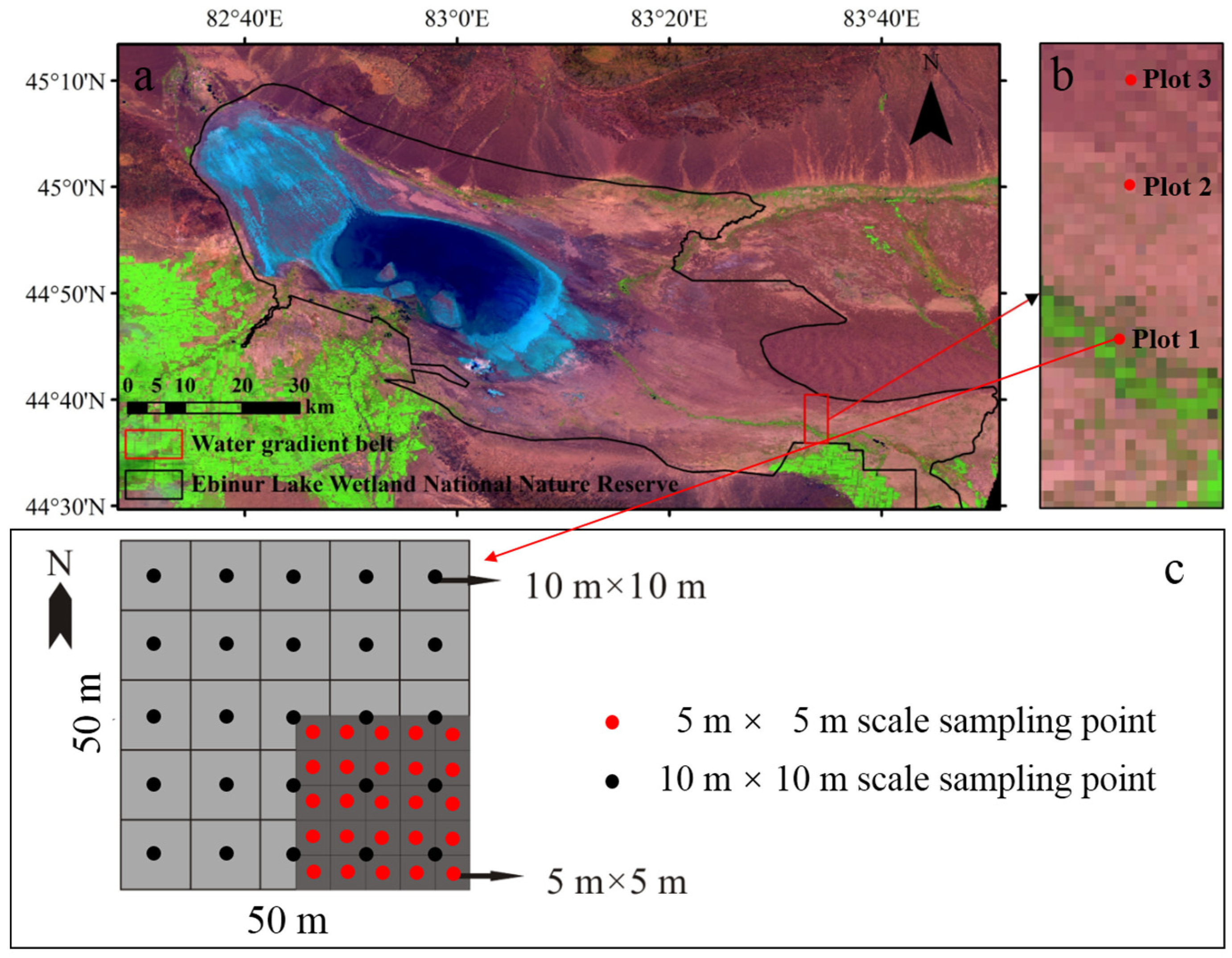
2.1. Study Site

The Ebinur Lake Wetland National Nature Reserve is located in the northwest of Xinjiang Uygur Autonomous Region, Bortala Mongolian Autonomous Prefecture (44°37′05′′–45°10′35′′ N, 82°30′47′′–83°50′21′′ E), and has a temperate continental arid climate. The average annual temperature is 6–8 °C, the annual precipitation is approximately 100 mm, the annual evaporation is approximately 1600 mm, and the groundwater depth is 1.8−2.7 m. The Ebinur Lake Wetland National Nature Reserve is mainly composed of eight soil types (Figure S1), dominated by silt and clay [51,52]. The main plant types are Haloxylon ammodendron (C.A.M.) Bge., Populus euphratica Oliv., Tamarix ramosissima Ldb., and Phragmites australis (Cav.) Trin. ex Steud.

2.2. Experimental Design

The water gradient zone is 8 km long, north of the Aqikesu River, and perpendicular to the riparian zone [55]. The climatic conditions in the gradient zone are relatively uniform, and there is little difference in topography and altitude. In August 2013, three 5 km long transects were established on the water gradient zone at intervals of 5 km [56]. According to the groundwater level and vegetation development, the gradient belt from southwest to northeast can be divided into riverbank habitat, transitional zone habitat, and desert margin habitat [19]. The riverbank habitat is located at the southern end of the gradient zone (0~1.50 km from the riparian zone), and the groundwater table is relatively shallow due to its proximity to the channel. The main plant species are Populus euphratica, Halimodendron halodendron, and Phragmites australis, and the soil nutrients and biomass are higher than in other regions [57]. The transitional zone habitat is located in the middle of the gradient zone (1.50~4.50 km from the riparian zone), and suitable water content maintains the symbiosis of 17 plants, including Reaumuria soongorica (Pall.) Maxim. and Aeluropus pungens (M. Bieb.) C. Koch. The desert margin habitat is at the northernmost end of the gradient zone (4.50~8.00 km from the riparian zone). The soil particle size is large, the organic matter content (1.35 g kg−1) is low, and the soil water content (1.04%) is also low, making plant survival challenging. The species growing in this area mainly include Haloxylon ammodendron, Nitraria tangutorum, and Suaeda salsa [19].
In mid-July 2018, one of the three replicate transects was selected, and a 50 m × 50 m plot was established in each of the three habitats of this transect, namely plot 1, plot 2, and plot 3 (Figure 1). The nested sampling design method was used to systematically divide each plot according to the sampling scales of 10 m × 10 m and 5 m × 5 m, respectively [48,49]. For the vegetation survey, Rs monitoring, soil sampling, and plant sample collection, 25 grids were evenly set at each scale. First, the 50 m × 50 m plot was equally spaced into 25 grids of 10 m × 10 m. Then, the vertices of each grid were marked and fixed with PVC pipes as corner stakes, and the midpoint of four boundary lines of each 10 m × 10 m quadrat was measured by a ruler, and each quadrat was further divided into four grids of 5 m × 5 m. Finally, a total of 150 grids (150 grids = 25 grids × two sampling scales × three plots) were established in the three plots. The latitude, longitude, altitude, and other geographic information for each sample plot were recorded by handheld GPS, and each grid was numbered. Due to the negative effects of large-scale destructive soil sampling and expensive labor and time costs, it was impossible to test in all transects [58]. In addition, according to the findings of the previous research group, there were no significant differences in plant composition and soil properties among the three replicate transects (Table S1) [56]. Therefore, we hypothesized that our experimental design could reflect the response of Rs to habitat changes (water gradients) at different spatial scales. This non-repeated experimental design method has been widely used to study the spatial variability of Rs on the fine scale [58,59,60,61].

2.3. Rs and Soil Indicators

The center point of each 10 m × 10 m and 5 m × 5 m grid was taken as the Rs measurement point. To reduce the influence of human disturbance and plant photosynthesis on the Rs measurement results, a PVC collar (inner diameter: 20 cm, height: 15 cm) was placed one day in advance at the center of each grid to measure Rs (150 collars in total). The PVC collar was then vertically embedded into the soil until its surface was approximately 5 cm above ground level, and living plants inside the collar were removed. A period of sunny and windless weather was selected from mid-July to mid-August in 2018, and the Rs and ST were measured by an LI-8100 portable gas analysis system (LI-COR Inc., Lincoln, NE, USA) at 10:00–12:00 (local time) every day. The 10 m × 10 m sampling scale was measured before the 5 m × 5 m sampling scale. To eliminate the influence of above-ground plant respiration, the ground vegetation and large branches in the collar were all removed one day before the measurement [19]. Each PVC collar was measured three times, and the average value was taken as the Rs value at the measuring point [22,60]. Rs was measured and the 0–10 cm ST was measured by a thermocouple temperature probe with an LI-8100 instrument (LI-COR Inc., Lincoln, NE, USA).
After the surface litter was removed near each Rs monitoring point, soil samples of 0–10 cm were collected. Two soil samples were taken, and one soil sample was collected by aluminum box (the aluminum box was weighed in advance). After the aluminum box soil was collected, it was numbered and weighed to obtain its fresh weight. It was then brought back to the laboratory to determine the SWC by the drying method [61]. Another soil sample was dried, and debris was removed using a 2-mm sieve for later soil index determination. Soil pH was determined using a PHS-3C Precision pH meter (Shanghai Etorch Electro-Mechanical Technology Co., Ltd., Shanghai, China). The soil organic carbon (SOC), total nitrogen (TN), nitrate nitrogen (NN), ammonium nitrogen (AN), total phosphorus (TP), and available phosphorus (AP) were measured using the methods described by Wang et al. [19].

2.4. Community Survey and Plant Functional Trait Measurement

Community surveys were performed in each 5 m × 5 m and 10 m × 10 m grid throughout the period of Rs measurements. This process included recording the species names and measuring the plant number, coverage, and height of each species. According to the global functional characteristics measurement manual and combined with the vegetation characteristics in the study area, nine functional traits were selected, including leaf length (LL), leaf width (LW), leaf thickness (LT), maximum plant height (Hmax), specific leaf area (SLA), leaf dry matter content (LDMC), leaf carbon content (LCC), leaf nitrogen content (LNC), and leaf phosphorus content (LPC) [62]. For each plant appearing in the grid, 30–50 fully developed, and healthy leaves were collected to measure the leaf traits [62]. LL (mm), LW (mm), and LT (mm) were measured by Vernier calipers with an accuracy of 0.01 mm. ImageJ was used to calculate leaf area after scanning all collected leaves [63]. The leaves were then placed in an oven at 80 °C for 48 h and immediately weighed with an electronic balance with an accuracy of 0.001 g. SLA (m2 kg−1) is defined as the ratio of leaf area (m2) to leaf dry weight (kg). LDMC (%) is defined as the ratio of leaf dry weight (kg) to leaf fresh weight (kg). Finally, all dried plant leaves were ground and stored in self-sealing bags for the determination of leaf element contents. LPC, LNC, and LCC were determined by the molybdenum antimony resistance colorimetric method, H2SO4-H2O2-Kjeldahl method, and potassium dichromate dilution method, respectively [64].

2.5. Statistical Analyses

The coefficient of variation (CV) was calculated by standard deviation (SD)/mean value (mean) to represent the spatial variation of Rs and environmental factors. CV < 10% was considered weak variability, 10% < CV < 100% was considered moderate variability, and CV > 100% was considered strong variability [42]. Differences in Rs, soil properties, and plant traits between the two sampling scales were analyzed using independent-samples t-tests. Two-factor analysis of variance (ANOVA) was used to analyze the effects of plot type and sampling scale on Rs. Rs was converted into a natural logarithm before analysis to achieve normal distribution. GS+ 9.0 (Gamma Design Software, Plainwell, MI, USA) geostatistics software was used for semi-variance function model fitting and parameter calculation. The ratio C/(C0 + C) of partial sill and sill was used to reflect the spatial autocorrelation of Rs. C/(C0 + C) > 75%, 25%–75%, and <25% indicated strong, moderate, and weak spatial autocorrelation of Rs, respectively [65]. The ggpmisc package was used to conduct fitting regression analysis of Rs and the environmental factors (soil microclimate, soil nutrients, and plant traits) of the three plots. Due to the collinearity among environmental factors, the Hmisc package varclus function was used to cluster and evaluate the redundancy among environmental factors before the multiple regression analysis, and the factors with high correlation were removed [66].
The Vegan package varpart function was used to perform variance partitioning analysis (VPA) based on redundancy analysis (RDA) to assess the explanatory degree of different types of environmental factors (e.g., soil microclimate, soil nutrients, and plant traits) on the spatial change of Rs [67]. Before RDA analysis, to improve the normality and homogeneity of the variance of data, all environmental factors were log transformed. Then, the ordistep function was used for backward selection to delete the variables that were not significant in each explanatory set. Finally, 999 Monte Carlo permutation tests were performed on the RDA analysis results to quantitatively evaluate the contribution rates of different types of environmental factors to the spatial variation of Rs (i.e., the independent explanatory variables). To prevent overfitting, the adjusted R2 was selected as the recognition criterion to evaluate the interpretation ability of the model.

3. Results

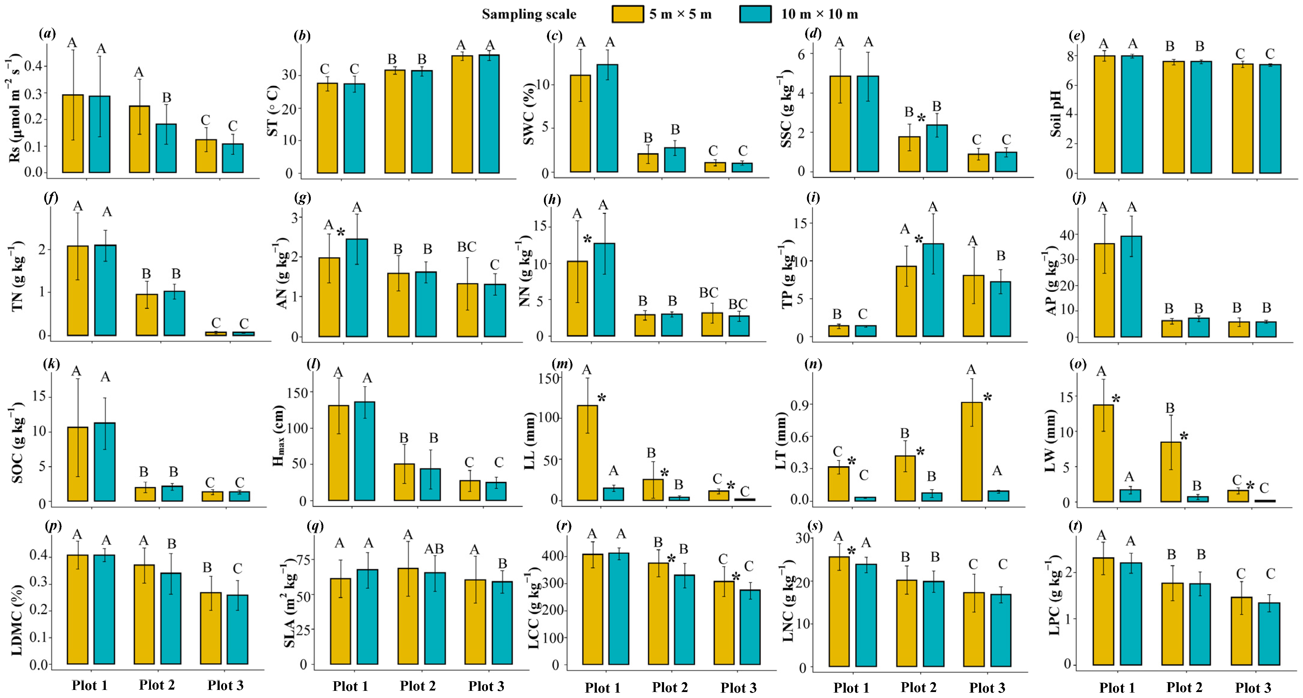
3.1. Changes in Rs and Environmental Factors

The mean Rs of plot 1 was the highest (5 m × 5 m: 0.29 ± 0.17 μmol m−2 s−1; 10 m × 10 m: 0.28 ± 0.15 μmol m−2 s−1), and that of plot 3 was the lowest (5 m × 5 m: 0.12 ± 0.05 μmol m−2 s−1; 10 m × 10 m: 0.11 ± 0.04 μmol m−2 s−1) (Figure 2a). Plot types had significant effects on Rs, but sampling scales and their interactions with plot types had no significant effects on Rs (p > 0.05, Table 1). At different sampling scales, ST, SWC, SSC, pH, TN, SOC, Hmax, and LPC were not significantly different in the same plot (p > 0.05, Figure 2b–f), but were significantly different among the three plots (p < 0.05, Figure 2k,l,t). At the sampling scale of 5 m × 5 m, the AN, NN, TP, and AP of plot 1 were significantly higher than those of plot 2 and plot 3 (p < 0.05, Figure 2g–j), while there was no significant difference in AN, NN, TP, and AP between plot 2 and plot 3 (p > 0.05). At the sampling scale of 10 m × 10 m, except for AP and SLA, the variables showed significant differences among different plots (p < 0.05, Figure 2q). LW, LT, and LL were significantly different among different plots and sampling scales (p < 0.05, Figure 2m–o).
In addition to ST and pH, Rs and its environmental factors exhibited moderate spatial variations (10% ≤ CV ≤ 100%). Among them, the CV of Rs and environmental factors at different scales were not significantly different in three plots, but were different among different plots, showing the order of plot 1 > plot 2 > plot 3 (Table 2). At the sampling scale of 5 m × 5 m, Rs in plot 1, plot 2, and plot 3 had strong, medium, and weak spatial dependence, respectively. At the scale of 10 m × 10 m, the spatial dependence of Rs in plot 1 and plot 2 was stronger, while that in plot 3 was weaker (Table 3).

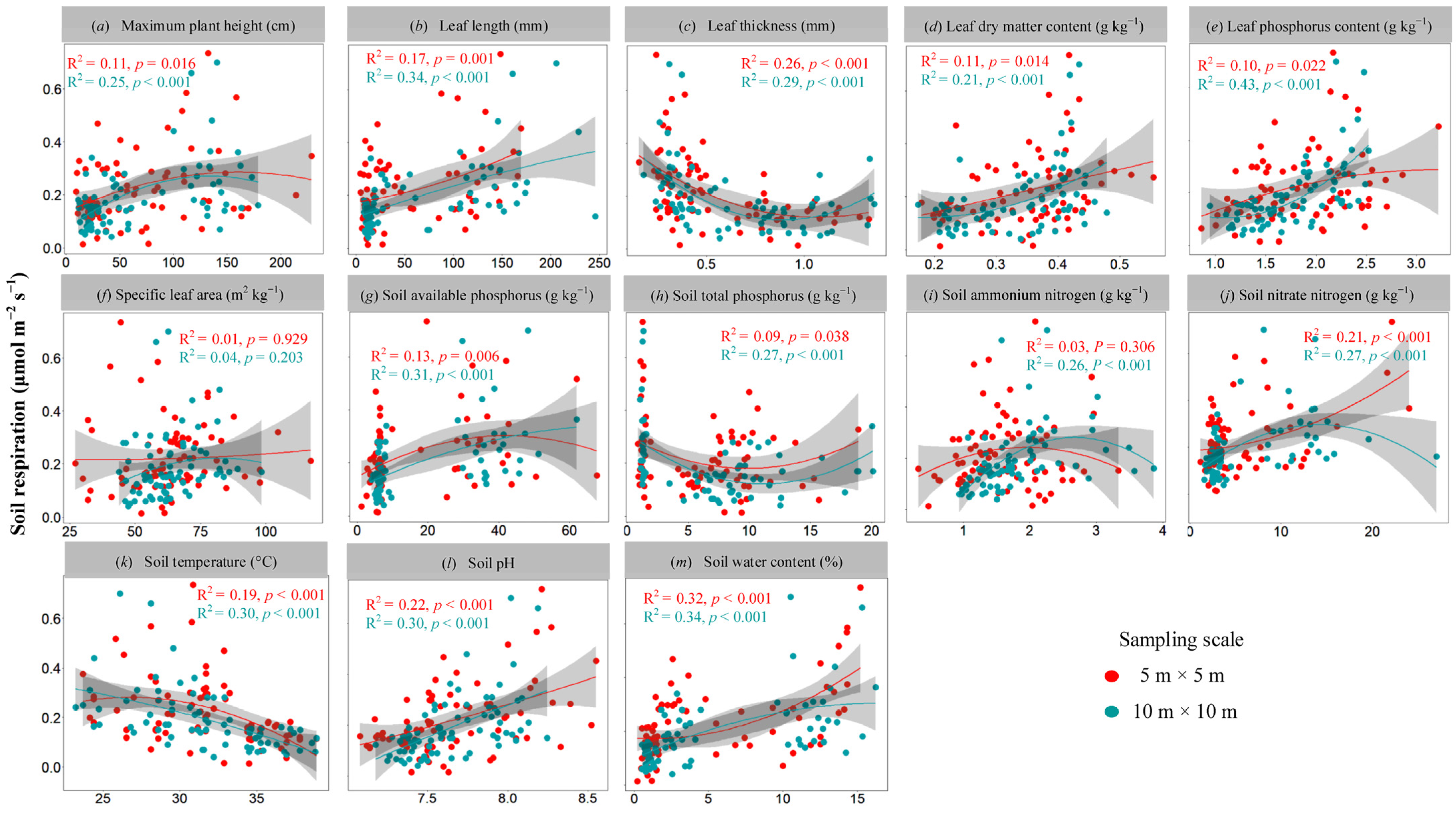
3.2. Multiple Regression Analysis of Rs and Environmental Factors in Specific Plot Types under Different Sampling Scales

The variables with higher correlations (LW, LC, LN, TN, SSC, and SOC) were removed because of Spearman’s ρ2 > 0.7 (Figure S2), and all the other variables were entered into the final model. Under different sampling scales, the most significant environmental variables affecting the spatial variation of Rs in different plots could be explained by the multiple regression analysis model (Table S2). At the scale of 5 m × 5 m, LL (0.02, p < 0.01), LDMC (2.98, p < 0.01), LPC (0.52, p < 0.001), and AP (0.01, p < 0.05) jointly explained 49% of Rs variation in plot 1. In plot 2, LPC had the most significant effect on Rs (0.12, p < 0.05). As the most significant variables affecting the Rs in plot 3, LL (−0.06, p < 0.05), LT (−1.23, p < 0.05), and AN (0.07, p < 0.01) jointly explained 42% of the total variation (p < 0.005). At the scale of 10 m × 10 m, LL (partial regression coefficient was 0.01, p < 0.05), SWC (0.04, p < 0.001), and pH (0.19, p < 0.01) were the most important variables affecting the Rs in plot 1, which could explain 70% of the spatial variation of the Rs in this plot (p < 0.001). The contribution of LPC, SWC, TP, and AN to the Rs in plot 2 was small but significant (−0.09–0.06, p < 0.05). In contrast, SWC had a unique effect on the spatial change of Rs in plot 3 (0.08, p < 0.001) that explained 36% of the total variation in this plot (p < 0.001).

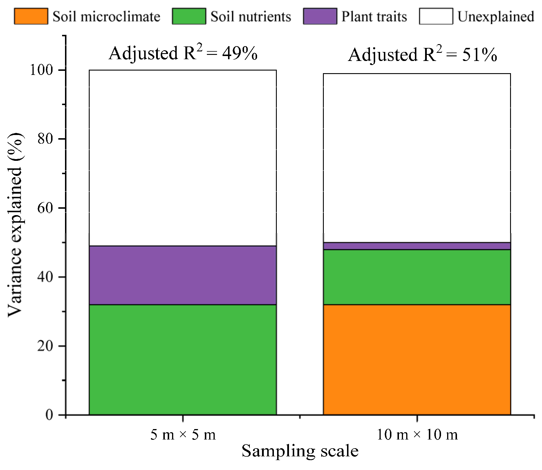
3.3. The Influencing Factors of Rs among Three Plot Types under Different Sampling Scales

Figure 3 displays the regression relationship between Rs and several environmental factors at different sampling scales. Among them, the relationships between Rs and SLA, TP, and AN were weak at the 5 m × 5 m scale (p > 0.05, Figure 3f,i), and the relationship between Rs and other factors was more obvious (p < 0.05, Figure 3). At the 10 m × 10 m scale, except for SLA, other influencing factors were significantly correlated with Rs (p < 0.05, Figure 3).
The results of RDA and variation partitioning showed that plant traits (Hmax, LL, and LP) at the 5 m × 5 m scale explained 17% of the spatial variation of Rs, and soil nutrients (AP and NN) and plant traits explained 49% of the spatial variation (Figure 4). At the sampling scale of 10 m × 10 m, soil microclimate (SWC), soil nutrients (pH, AP, and NN) and plant traits (LT) jointly explained 51% of the spatial variation of Rs. Among them, soil microclimate and soil nutrients accounted for a large proportion (32% and 16%, respectively), and plant traits explained 3% of the variation of Rs. The spatial change of Rs explained by soil nutrients and plant traits at both scales was significant (p < 0.05), while soil microclimate only explained a large part of the variation of Rs at the 10 m × 10 m scale (p < 0.05).

4. Discussion

The results showed that the CV of Rs in plot 1 was the largest, and the CVs of soil properties and plant functional traits were greater than those in plot 2 and plot 3 (Table 2). The above results suggest that the biotic and abiotic factors in plot 1 had higher variability than those in plot 2 and plot 3, which might lead to stronger spatial variability of Rs by affecting plant and soil conditions [22,30]. At different spatial scales, Rs exhibits high variability [62,63,64]. Voroney and Russell [65] sampled a mature birch forest along a 40 m sampling line at 2–4 m intervals and found that the CV of Rs was between 16% and 45%. Rayment and Jarvis [66] reported that when the sampling scale was greater than 1 m, the spatial variation of Rs increased with the increase of sampling spacing, but the increase was not significant. Kosugi et al. [48] suggested that the CV of the Rs rate increased with the increase of spatial grain size (5 m × 5 m, 10 m × 10 m, and 50 m × 50 m). However, there was no difference in the variation coefficient of Rs between the 5 m × 5 m and 10 m × 10 m scales. Adachi et al. [67] measured the variation coefficients of Rs at 20 m × 20 m sampling scales of 1 hm2 and 2 hm2 and obtained CV values of 42.3%–43.7% and 39.6%–44.5%, respectively. In the present study, it was found that although Rs had obvious spatial variation, the variation coefficients of Rs in the same plot were consistent at two sampling scales (Figure 2 and Table 2). This indicates that relatively stable environmental factors at different sampling scales control the spatial variability of high or low Rs in the same plot [42,68]. The spatial autocorrelation ranges of Rs at the 5 m × 5 m and 10 m × 10 m sampling scales were 11.65–16.3 m and 15.45–32.60 m, respectively, which were consistent with the results of Kosugi et al. [48] (i.e., the spatial autocorrelation ranges of Rs were 7.9–14.1 m). These results indicate that it is important to evaluate the changes of Rs at different scales and analyze the key factors affecting the changes [19].
Rs includes autotrophic respiration (Ra) and heterotrophic respiration (Rh) [69]. Ra reflects carbon returned from roots and associated microbes to the atmosphere and regulates the distribution of photosynthetic carbon to underground tissues [29], namely root-derived respiration (i.e., root respiration and root exudates) [28]. Rh reflects the CO2 released by the microbial decomposition of organic matter [69]. Therefore, Rs connects aboveground and underground carbon fractions [70] in terrestrial ecosystems and is significantly associated with a series of aboveground and underground plant traits and soil properties. However, it is difficult for researchers to obtain information on underground plant traits involving a certain spatial range. Because there is a strong correlation between changes in aboveground and underground traits [38], it is feasible to select easily measured aboveground functional traits to predict spatial variations in Rs [71]. The results showed that the key factors affecting Rs variability differed at different spatial scales. The effects of driving factors on Rs were significantly different, and plant functional traits could explain some variations in Rs (Table S2). This is because variations in aboveground plant traits can affect litter decomposition rates [72], soil microbial communities [73], and soil nutrient cycling [74,75], and they can directly and indirectly affect spatial changes in Rs [76]. When spatial scales change, the controlling factors of Rs variation at small scales may be replaced by factors that have a stronger impact at the large scale [68]. Martin and Bolstad [41] suggested that the spatial variation of Rs at the 0–1 m2 scale was mainly affected by roots and litter, while at the scale of 1–100 m2, it was mainly affected by root biomass, soil carbon/nitrogen content, and root nitrogen content. At the landscape scale, topography strongly affects soil moisture and soil properties and causes great changes in the spatial pattern of Rs. Shi and Jin [68] reported that the variation of Rs in a forest type in northeast China depended on forest structure parameters (mean diameter at breast height, maximum diameter at breast height, and total basal area) and soil physical and chemical properties (water-filled porosity, soil organic carbon content, and soil C:N). Soil physical and chemical properties (soil organic carbon content, soil C:N, and field capacity) control the variation of Rs among four forest types. A previous study has shown that the size of biomass controls the spatial distribution of Rs, while the effects of ST and SWC are relatively small [77]. However, biomass and plant diversity are related to the increase of root biomass, and root biomass regulates Rs in natural systems in the interaction with ST and SWC [36]. In this study, it was found that at the scale of 5 m × 5 m, the spatial variation of Rs in the three plots mainly depended on plant traits (LL, LT, LDMC, and LPC, p < 0.05), while at the scale of 10 m × 10 m, the spatial variation of Rs in the three plots mainly depended on soil properties (TP, AN, SWC, and pH, p < 0.05). The above results showed that the differences in biotic (plant functional traits) and abiotic factors (soil properties) increased correspondingly with the increase of the sampling scale, which may have been caused by the differences in soil physical and chemical properties and functional traits caused by plant community composition and vegetation patch distribution [23,28,78].
Xu and Qi [19] showed that the spatial change of Rs was related to root and microbial biomass, soil physical and chemical properties, ST, and SWC. As water decreases, the soil becomes barren, resulting in a gradual decrease in Rs. In the present study, soil nutrients and plant traits at two sampling scales jointly controlled the variation of Rs at the local scale (p < 0.05). The mean Rs of plot 3 was the lowest at any sampling scale (Figure 2a). This is because soil nutrients are the material basis for plant growth and soil microbial survival, and their content determines the growth and development of plants and the size of the microbial biomass [79]. The leaf is the site of plant photosynthesis, and the length, width, size, and thickness of leaves affect photosynthesis. Studies have shown that root respiration and photosynthesis have a strong coupling relationship [33], and the photosynthetic rate largely affects root activity. Plant leaves adapt to changes in the external environment, such as drought stress, by changing their physical forms [55], such as by changing the distribution of photosynthetic products to roots, leading to changes in soil autotrophic respiration [31,80]. Therefore, compared with plot 3, plot 1, with high photosynthesis and biomass, also had relatively strong Rs [57,81]. In future studies, the community functional parameters of plant functional traits and the influence mechanism of plant functional trait diversity on Rs should be focused on [19].
Studies have shown that SWC is very important among the various factors affecting the spatial variation of Rs [48,82]. The direct effect of SWC on Rs occurred through the physiological processes of roots and microorganisms, and the indirect effect on Rs occurred through the diffusion of substrate and oxygen [83,84]. A study by Cai et al. [17] in Kayanodaira Forest, Japan, found that the spatial variability of SRdaily (daily summed Rs) was well correlated with SWC, and SRdaily first increased and then decreased with the increase of SWC. Jiang et al. [62] showed that the spatial distribution of the Rs rate was significantly negatively correlated with SWC in subtropical evergreen broad-leaved forests in southern China. The results of the present study showed (Figure 3) that the variation of Rs at the local scale could be well explained by SWC (5 m × 5 m: R2 = 0.32; 10 m × 10 m: R2 = 0.34). In addition, compared with the sampling scale of 5 m × 5 m, the large spatial variation of Rs at the scale of 10 m × 10 m could be explained by SWC (Figure 4, p < 0.05). This is because SWC, at levels that are too low or too high, limits Rs [85], especially in arid or semi-arid areas. When SWC becomes a stress factor, it may replace temperature and become the main control factor of the Rs rate [19,86]. The effect of SWC on Rs is very complex and changeable. When the soil is dry, the soil metabolic activity increases with the increase of water content, and there is a positive correlation between them. When SWC exceeds a certain range (80% of saturated soil moisture), the Rs decreases with the increase of SWC, and there is a negative correlation between them [36,87]. These results indicated that the synergistic changes of plant functional traits and soil nutrients with SWC caused the spatial variation of the Rs rate at the local scale. Therefore, to improve the uncertainty of existing models for predicting Rs and better elucidate the potential mechanism of the spatial pattern of Rs in arid areas, it is necessary to quantify the spatial variation of Rs and its relationship with related environmental factors (plant traits, soil nutrients, and soil microclimate) at a fine scale (10 m × 10 m).

5. Conclusions

We have provided valid and reliable evidence that, with increasing sampling scale, the spatial variability of Rs was primarily influenced by soil properties, followed by plant traits, the relative importance of which depends on soil water conditions. In addition, the contribution of soil properties varies with plot types, and its influence in plot 1 (riverbank habitat) was greater than that in plot 3 (desert margin habitat). Among them, soil microclimate has a greater potential to enhance the spatial heterogeneity of Rs than soil nutrients. These results emphasize that the nested sampling design method can be used to quantify the relationship between Rs and related driving factors at different spatial scales in regions with large soil water changes, which can help inform the design of Rs field sampling schemes at local scales.

Supplementary Materials

The following supporting information can be downloaded at: https://0-www-mdpi-com.brum.beds.ac.uk/article/10.3390/f13071001/s1, Table S1: Comparison in soil properties of the measuring transect (transect 1) and the other two transects (transects 2–3); Figure S1: Soil types in the Ebinur Lake Wetland National Nature Reserve; Table S2: Multiple regression analysis of soil respiration and related influencing factors within the same plot. Hmax: Maximum plant height; LL: Leaf length; LT: Leaf thickness; LDMC: Leaf dry matter content; SLA: Specific leaf area; LPC: Leaf phosphorus content; SWC: Soil water content; ST: Soil temperature; pH: Soil pH; AP: Soil available phosphorus; TP: Soil total phosphorus; AN: Soil ammonium nitrogen; NN: Soil nitrate nitrogen; NS, not significant; ND, not determined (removed by the stepwise regression analysis results). * p < 0.05, ** p < 0.01, *** p < 0.001; Figure S2: Cluster analysis of the measured environmental variables. Hmax: Maximum plant height; LL: Leaf length; LW: Leaf width; LT: Leaf thickness; LDMC: Leaf dry matter content; SLA: Specific leaf area; LPC: Leaf phosphorus content; LNC: Leaf nitrogen content; LCC: Leaf carbon content; SWC: Soil water content; ST: Soil temperature; pH: Soil pH; AN: Soil ammonium nitrogen; AP: Soil available phosphorus; TP: Soil total phosphorus; TN: Total nitrogen content; NN: Soil nitrate nitrogen; SSC: Soil salinity content.

Author Contributions

Conceptualization, J.W. and G.L.; methodology, J.W.; software, J.W.; data curation, Z.L. and Y.C.; writing—original draft preparation, J.W.; writing—review and editing, X.H. and W.M.; supervision, G.L.; funding acquisition, G.L. and X.H. All authors have read and agreed to the published version of the manuscript.

Funding

This research was funded by the National Natural Science Foundation of China (31560131 and 31760168), Xinjiang Uygur Autonomous Region university scientific research project (XJEDU2020I002), Xinjiang Uygur Autonomous Region Innovation Environment Construction Project—Science and Technology Innovation Base Construction Project (PT2107), and the Xinjiang Uygur Autonomous Region Graduate Research and Innovation Project (XJ2020G012 and XJ2019G020).

Institutional Review Board Statement

Not applicable.

Informed Consent Statement

Not applicable.

Data Availability Statement

The data presented in this study are available on request from the corresponding author.

Acknowledgments

We are grateful to Xueni Zhang of Xinjiang University’s College of Ecology and Environment for providing the data. We also thank the editor and the reviewers for their insightful and valuable suggestions, which greatly improved the quality of this manuscript.

Conflicts of Interest

The authors declare no conflict of interest.

References

  1. Hashimoto, S.; Carvalhais, N.; Ito, A.; Migliavacca, M.; Nishina, K.; Reichstein, M. Global spatiotemporal distribution of soil respiration modeled using a global database. Biogeosciences 2015, 12, 4121–4132. [Google Scholar] [CrossRef] [Green Version]
  2. Nunes, M.R.; Karlen, D.L.; Veum, K.S.; Moorman, T.B.; Cambardella, C.A. Biological soil health indicators respond to tillage intensity: A US meta-analysis. Geoderma 2020, 369, 114335. [Google Scholar] [CrossRef]
  3. Pries, C.E.H.; Castanha, C.; Porras, R.C.; Torn, M.S. The whole-soil carbon flux in response to warming. Science 2017, 355, 1420–1423. [Google Scholar] [CrossRef] [PubMed] [Green Version]
  4. Lei, J.; Guo, X.; Zeng, Y.; Zhou, J.; Gao, Q.; Yang, Y. Temporal changes in global soil respiration since 1987. Nat. Commun. 2021, 12, 403. [Google Scholar] [CrossRef] [PubMed]
  5. Adachi, M.; Ito, A.; Yonemura, S.; Takeuchi, W. Estimation of global soil respiration by accounting for land-use changes derived from remote sensing data. J. Environ. Manag. 2017, 200, 97–104. [Google Scholar] [CrossRef] [Green Version]
  6. Fóti, S.; Balogh, J.; Herbst, M.; Papp, M.; Koncz, P.; Bartha, S.; Zimmermann, Z.; Komoly, C.; Szabó, G.; Margóczi, K.; et al. Meta-analysis of field scale spatial variability of grassland soil CO2 efflux: Interaction of biotic and abiotic drivers. CATENA 2016, 143, 78–89. [Google Scholar] [CrossRef] [Green Version]
  7. Schlesinger, W.H.; Andrews, J.A. Soil respiration and the global carbon cycle. Biogeochemistry 2000, 48, 7–20. [Google Scholar] [CrossRef]
  8. Hursh, A.; Ballantyne, A.; Cooper, L.; Maneta, M.; Kimball, J.; Watts, J. The sensitivity of soil respiration to soil temperature, moisture, and carbon supply at the global scale. Glob. Chang. Biol. 2016, 23, 2090–2103. [Google Scholar] [CrossRef]
  9. Tang, X.; Du, J.; Shi, Y.; Lei, N.; Chen, G.; Cao, L.; Pei, X. Global patterns of soil heterotrophic respiration—A meta-analysis of available dataset. CATENA 2020, 191, 104574. [Google Scholar] [CrossRef]
  10. Stephan, E.; Groffman, P.; Vidon, P.; Stella, J.C.; Endreny, T. Interacting drivers and their tradeoffs for predicting denitrification potential across a strong urban to rural gradient within heterogeneous landscapes. J. Environ. Manag. 2021, 294, 113021. [Google Scholar] [CrossRef]
  11. Riutta, T.; Kho, L.K.; Teh, Y.A.; Ewers, R.; Majalap, N.; Malhi, Y. Major and persistent shifts in below-ground carbon dynamics and soil respiration following logging in tropical forests. Glob. Chang. Biol. 2021, 27, 2225–2240. [Google Scholar] [CrossRef] [PubMed]
  12. Ouyang, W.; Lai, X.; Li, X.; Liu, H.; Lin, C.; Hao, F. Soil respiration and carbon loss relationship with temperature and land use conversion in freeze-thaw agricultural area. Sci. Total Environ. 2015, 533, 215–222. [Google Scholar] [CrossRef] [PubMed]
  13. Zhang, Y.; Zou, J.; Dang, S.; Osborne, B.; Ren, Y.; Ju, X. Topography modifies the effect of land-use change on soil respiration: A meta-analysis. Ecosphere 2021, 12, e03845. [Google Scholar] [CrossRef]
  14. Han, G.; Yu, J.; Li, H.; Yang, L.; Wang, G.; Mao, P.; Gao, Y. Winter Soil Respiration from Different Vegetation Patches in the Yellow River Delta, China. Environ. Manag. 2012, 50, 39–49. [Google Scholar] [CrossRef]
  15. Jian, J.; Steele, M.K.; Zhang, L.; Bailey, V.L.; Zheng, J.; Patel, K.F.; Bond-Lamberty, B.P. On the use of air temperature and precipitation as surrogate predictors in soil respiration modelling. Eur. J. Soil Sci. 2021, 73, e13149. [Google Scholar] [CrossRef]
  16. Darenova, E.; Čater, M. Different Structure of Sessile Oak Stands Affects Soil Moisture and Soil CO2 Efflux. For. Sci. 2018, 64, 340–348. [Google Scholar] [CrossRef]
  17. Cai, Y.; Nishimura, T.; Ida, H.; Hirota, M. Spatial variation in soil respiration is determined by forest canopy structure through soil water content in a mature beech forest. For. Ecol. Manag. 2021, 501, 119673. [Google Scholar] [CrossRef]
  18. Lee, J.-S. Relationship of root biomass and soil respiration in a stand of deciduous broadleaved trees—A case study in a maple tree. J. Ecol. Environ. 2018, 42, 19. [Google Scholar] [CrossRef]
  19. Wang, J.; Teng, D.; He, X.; Qin, L.; Yang, X.; Lv, G. Spatial non-stationarity effects of driving factors on soil respiration in an arid desert region. CATENA 2021, 207, 105617. [Google Scholar] [CrossRef]
  20. Tang, Y.-S.; Wang, L.; Jia, J.-W.; Fu, X.-H.; Le, Y.-Q.; Chen, X.-Z.; Sun, Y. Response of soil microbial community in Jiuduansha wetland to different successional stages and its implications for soil microbial respiration and carbon turnover. Soil Biol. Biochem. 2011, 43, 638–646. [Google Scholar] [CrossRef]
  21. Yang, J.; Zhan, C.; Li, Y.; Zhou, D.; Yu, Y.; Yu, J. Effect of salinity on soil respiration in relation to dissolved organic carbon and microbial characteristics of a wetland in the Liaohe River estuary, Northeast China. Sci. Total Environ. 2018, 642, 946–953. [Google Scholar] [CrossRef] [PubMed]
  22. Singh, R.; Singh, A.K.; Singh, S.; Srivastava, P.; Singh, H.; Raghubanshi, A.S. Geomorphologic heterogeneity influences dry-season soil CO2 efflux by mediating soil biophysical variables in a tropical river valley. Aquat. Sci. 2019, 81, 43. [Google Scholar] [CrossRef]
  23. Raich, J.W.; Schlesinger, W.H. The global carbon dioxide flux in soil respiration and its relationship to vegetation and climate. Tellus B Chem. Phys. Meteorol. 1992, 44, 81–99. [Google Scholar] [CrossRef] [Green Version]
  24. Tang, J.; Baldocchi, D.D. Spatial-Temporal variation in soil respiration in an oak-grass savanna ecosystem in California and its partitioning into autotrophic and heterotrophic components. Biogeochemistry 2005, 73, 183–207. [Google Scholar] [CrossRef]
  25. Xu, M.; Qi, Y. Soil-surface CO2 efflux and its spatial and temporal variations in a young ponderosa pine plantation in northern California. Glob. Chang. Biol. 2001, 7, 667–677. [Google Scholar] [CrossRef] [Green Version]
  26. Janssens, I.A.; Pilegaard, K. Large seasonal changes in Q 10 of soil respiration in a beech forest. Glob. Chang. Biol. 2003, 9, 911–918. [Google Scholar] [CrossRef]
  27. Tang, J.; Baldocchi, D.; Qi, Y.; Xu, L. Assessing soil CO2 efflux using continuous measurements of CO2 profiles in soils with small solid-state sensors. Agric. For. Meteorol. 2003, 118, 207–220. [Google Scholar] [CrossRef]
  28. Metcalfe, D.B.; Fisher, R.A.; Wardle, D.A. Plant communities as drivers of soil respiration: Pathways, mechanisms, and significance for global change. Biogeosciences 2011, 8, 2047–2061. [Google Scholar] [CrossRef] [Green Version]
  29. Högberg, P.; Nordgren, A.; Ågren, G.I. Carbon allocation between tree root growth and root respiration in boreal pine forest. Oecologia 2002, 132, 579–581. [Google Scholar] [CrossRef]
  30. Raich, J.W.; Tufekciogul, A. Vegetation and soil respiration: Correlations and controls. Biogeochemistry 2000, 48, 71–90. [Google Scholar] [CrossRef]
  31. Kuzyakov, Y.; Gavrichkova, O. REVIEW: Time lag between photosynthesis and carbon dioxide efflux from soil: A review of mechanisms and controls. Glob. Chang. Biol. 2010, 16, 3386–3406. [Google Scholar] [CrossRef]
  32. Atkin, O.K.; Edwards, E.J.; Loveys, B.R. Response of root respiration to changes in temperature and its relevance to global warming. New Phytol. 2000, 147, 141–154. [Google Scholar] [CrossRef]
  33. Högberg, P.; Nordgren, A.; Buchmann, N.; Taylor, A.F.S.; Ekblad, A.; Högberg, M.N.; Nyberg, G.; Ottosson-Löfvenius, M.; Read, D.J. Large-scale forest girdling shows that current photosynthesis drives soil respiration. Nature 2001, 411, 789–792. [Google Scholar] [CrossRef] [PubMed]
  34. Moyano, F.E.; Kutsch, W.L.; Schulze, E.-D. Response of mycorrhizal, rhizosphere and soil basal respiration to temperature and photosynthesis in a barley field. Soil Biol. Biochem. 2007, 39, 843–853. [Google Scholar] [CrossRef]
  35. De Deyn, G.B.; Cornelissen, J.H.C.; Bardgett, R.D. Plant functional traits and soil carbon sequestration in contrasting biomes. Ecol. Lett. 2008, 11, 516–531. [Google Scholar] [CrossRef]
  36. Kumari, T.; Singh, R.; Verma, P.; Raghubanshi, A.S. Monsoon-phase regulates the decoupling of auto- and heterotrophic respiration by mediating soil nutrient availability and root biomass in tropical grassland. CATENA 2021, 209, 105808. [Google Scholar] [CrossRef]
  37. Shen, Y.; Gilbert, G.S.; Li, W.; Fang, M.; Lu, H.; Yu, S. Linking Aboveground Traits to Root Traits and Local Environment: Implications of the Plant Economics Spectrum. Front. Plant Sci. 2019, 10, 1412. [Google Scholar] [CrossRef]
  38. Mao, W.; Felton, A.J.; Ma, Y.; Zhang, T.; Sun, Z.; Zhao, X.; Smith, M.D. Relationships between aboveground and belowground trait responses of a dominant plant species to alterations in watertable depth. Land Degrad. Dev. 2018, 29, 4015–4024. [Google Scholar] [CrossRef]
  39. Raich, J.W. Temporal patterns of soil respiration in tropical forest plantations in lowland Costa Rica. In Proceedings of the 96th ESA Annual Meeting, Austin, TX, USA, 7–12 August 2011. [Google Scholar]
  40. Jiang, Y.; Huang, X.; Zhang, X.; Zhang, X.; Zhang, Y.; Zheng, C.; Deng, A.; Zhang, J.; Wu, L.; Hu, S.; et al. Optimizing rice plant photosynthate allocation reduces N2O emissions from paddy fields. Sci. Rep. 2016, 6, 29333. [Google Scholar] [CrossRef] [Green Version]
  41. Martin, J.G.; Bolstad, P.V. Variation of soil respiration at three spatial scales: Components within measurements, intra-site variation and patterns on the landscape. Soil Biol. Biochem. 2009, 41, 530–543. [Google Scholar] [CrossRef]
  42. Chen, Q.; Wang, Q.; Han, X.; Wan, S.; Li, L. Temporal and spatial variability and controls of soil respiration in a temperate steppe in northern China. Glob. Biogeochem. Cycles 2010, 24, GB2010. [Google Scholar] [CrossRef]
  43. Buczko, U.; Bachmann, S.; Gropp, M.; Jurasinski, G.; Glatzel, S. Spatial variability at different scales and sampling requirements for in situ soil CO2 efflux measurements on an arable soil. CATENA 2015, 131, 46–55. [Google Scholar] [CrossRef]
  44. Wu, J.; Jones, B.; Li, H.; Loucks, O.L. Scaling and Uncertainty Analysis in Ecology: Methods and Applications; Springer: Dordrecht, The Netherlands, 2006. [Google Scholar]
  45. Jenerette, D.; Wu, J. On the Definitions of Scale. Bull. Ecol. Soc. Am. 2000, 81, 104–105. [Google Scholar] [CrossRef]
  46. Siefert, A.; Ravenscroft, C.; Althoff, D.; Alvarez-Yepiz, J.C.; Carter, B.E.; Glennon, K.L.; Heberling, M.; Jo, I.S.; Pontes, A.; Sauer, A.; et al. Scale dependence of vegetation-environment relationships: A meta-analysis of multivariate data. J. Veg. Sci. 2012, 23, 942–951. [Google Scholar] [CrossRef]
  47. Tamme, R.; Hiiesalu, I.; Laanisto, L.; Szava-Kovats, R.; Pärtel, M. Environmental heterogeneity, species diversity and co-existence at different spatial scales. J. Veg. Sci. 2010, 21, 796–801. [Google Scholar] [CrossRef]
  48. Kosugi, Y.; Mitani, T.; Itoh, M.; Noguchi, S.; Tani, M.; Matsuo, N.; Takanashi, S.; Ohkubo, S.; Nik, A.R. Spatial and temporal variation in soil respiration in a Southeast Asian tropical rainforest. Agric. For. Meteorol. 2007, 147, 35–47. [Google Scholar] [CrossRef]
  49. Zhang, M.; Li, G.; Liu, B.; Liu, J.; Wang, L.; Wang, D. Effects of herbivore assemblage on the spatial heterogeneity of soil nitrogen in eastern Eurasian steppe. J. Appl. Ecol. 2020, 57, 1551–1560. [Google Scholar] [CrossRef]
  50. Gong, G.L.X. Species diversity and dominant species’ niches of eremophyte communities of the Tugai forest in the Ebinur basin of Xinjiang, China. Biodivers. Sci. 2017, 25, 29–35. [Google Scholar] [CrossRef] [Green Version]
  51. Zerbe, S.; Halik, Ü.; Küchler, J. Urban greening in the oases of continental arid Southern Xinjiang (NW China)—An interdisciplinary approach. Erde 2005, 136, 245–266. [Google Scholar]
  52. Thevs, N.; Zerbe, S.; Schnittler, M.; Abdusalih, N.; Succow, M. Structure, reproduction and flood-induced dynamics of riparian Tugai forests at the Tarim River in Xinjiang, NW China. Forestry 2008, 81, 45–57. [Google Scholar] [CrossRef] [Green Version]
  53. Zhang, X.; Yang, X.; Lv, G. Diversity patterns and response mechanisms of desert plants to the soil environment along soil water and salinity gradients. Acta Ecol. Sin. 2016, 36, 3206–3215. [Google Scholar] [CrossRef]
  54. Leemans, R.; Eickhout, B. Another reason for concern: Regional and global impacts on ecosystems for different levels of climate change. Glob. Environ. Chang. 2004, 14, 219–228. [Google Scholar] [CrossRef]
  55. Gong, Y.; Ling, H.; Lv, G.; Chen, Y.; Guo, Z.; Cao, J. Disentangling the influence of aridity and salinity on community functional and phylogenetic diversity in local dryland vegetation. Sci. Total Environ. 2018, 653, 409–422. [Google Scholar] [CrossRef] [PubMed]
  56. Zhang, X.-N.; Yang, X.-D.; Li, Y.; He, X.-M.; Lv, G.-H.; Yang, J.-J. Influence of edaphic factors on plant distribution and diversity in the arid area of Xinjiang, Northwest China. Arid Land Res. Manag. 2017, 32, 38–56. [Google Scholar] [CrossRef]
  57. Wang, H.; Cai, Y.; Yang, Q.; Gong, Y.; Lv, G. Factors that alter the relative importance of abiotic and biotic drivers on the fertile island in a desert-oasis ecotone. Sci. Total Environ. 2019, 697, 134096. [Google Scholar] [CrossRef]
  58. Shi, B.; Xu, W.; Zhu, Y.; Wang, C.; Loik, M.E.; Sun, W. Heterogeneity of grassland soil respiration: Antagonistic effects of grazing and nitrogen addition. Agric. For. Meteorol. 2019, 268, 215–223. [Google Scholar] [CrossRef]
  59. Barba, J.; Yuste, J.C.; Martínez-Vilalta, J.; Lloret, F. Drought-induced tree species replacement is reflected in the spatial variability of soil respiration in a mixed Mediterranean forest. For. Ecol. Manag. 2013, 306, 79–87. [Google Scholar] [CrossRef]
  60. Liu, C.; Song, X.; Wang, L.; Wang, D.; Zhou, X.; Liu, J.; Zhao, X.; Li, J.; Lin, H. Effects of grazing on soil nitrogen spatial heterogeneity depend on herbivore assemblage and pre-grazing plant diversity. J. Appl. Ecol. 2016, 53, 242–250. [Google Scholar] [CrossRef]
  61. Yan, J.-X.; Sun, Q.; Li, J.-J.; Li, H.-J. Effect of the Sampling Scale and Number on the Heterogeneity of Soil Respiration in a Mixed Broadleaf-conifer Forest. Huan Jing Ke Xue = Huanjing Kexue 2019, 40, 383–391. [Google Scholar]
  62. Jiang, Y.; Zhang, B.; Wang, W.; Li, B.; Wu, Z.; Chu, C. Topography and plant community structure contribute to spatial heterogeneity of soil respiration in a subtropical forest. Sci. Total Environ. 2020, 733, 139287. [Google Scholar] [CrossRef]
  63. Han, M.; Shi, B.; Jin, G. Spatial patterns of soil respiration in a spruce-fir valley forest, Northeast China. J. Soils Sediments 2018, 19, 10–22. [Google Scholar] [CrossRef]
  64. Darenova, E.; Čater, M. Effect of spatial scale and harvest on heterogeneity of forest floor CO2 efflux in a sessile oak forest. CATENA 2020, 188, 104455. [Google Scholar] [CrossRef]
  65. Russell, C.A.; Voroney, R.P. Carbon dioxide efflux from the floor of a boreal aspen forest. I. Relationship to environmental variables and estimates of C respired. Can. J. Soil Sci. 1998, 78, 301–310. [Google Scholar] [CrossRef]
  66. Rayment, M.; Jarvis, P. Temporal and spatial variation of soil CO2 efflux in a Canadian boreal forest. Soil Biol. Biochem. 2000, 32, 35–45. [Google Scholar] [CrossRef]
  67. Adachi, M.; Bekku, Y.S.; Konuma, A.; Kadir, W.R.; Okuda, T.; Koizumi, H. Required sample size for estimating soil respiration rates in large areas of two tropical forests and of two types of plantation in Malaysia. For. Ecol. Manag. 2005, 210, 455–459. [Google Scholar] [CrossRef]
  68. Shi, B.; Jin, G. Variability of soil respiration at different spatial scales in temperate forests. Biol. Fertil. Soils 2016, 52, 561–571. [Google Scholar] [CrossRef]
  69. Subke, J.-A.; Inglima, I.; Cotrufo, M.F. Trends and methodological impacts in soil CO2 efflux partitioning: A metaanalytical review. Glob. Chang. Biol. 2006, 12, 921–943. [Google Scholar] [CrossRef]
  70. Tang, X.; Pei, X.; Lei, N.; Luo, X.; Liu, L.; Shi, L.; Chen, G.; Liang, J. Global patterns of soil autotrophic respiration and its relation to climate, soil and vegetation characteristics. Geoderma 2020, 369, 114339. [Google Scholar] [CrossRef]
  71. Cassart, B.; Basia, A.A.; Jonard, M.; Ponette, Q. Functional traits drive the difference in soil respiration between Gilbertiodendron dewevrei monodominant forests patches and Scorodophloeus zenkeri mixed forests patches in the Central Congo basin. Plant Soil 2021, 460, 313–331. [Google Scholar] [CrossRef]
  72. Garnier, E.; Cortez, J.; Billès, G.; Navas, M.-L.; Roumet, C.; Debussche, M.; Laurent, G.; Blanchard, A.; Aubry, D.; Bellmann, A.; et al. Plant functional markers capture ecosystem properties during secondary succession. Ecology 2004, 85, 2630–2637. [Google Scholar] [CrossRef]
  73. Pei, Z.; Eichenberg, D.; Bruelheide, H.; Kröber, W.; Kühn, P.; Li, Y.; von Oheimb, G.; Purschke, O.; Scholten, T.; Buscot, F.; et al. Soil and tree species traits both shape soil microbial communities during early growth of Chinese subtropical forests. Soil Biol. Biochem. 2016, 96, 180–190. [Google Scholar] [CrossRef]
  74. Fortunel, C.; Garnier, E.; Joffre, R.; Kazakou, E.; Quested, H.; Grigulis, K.; Lavorel, S.; Ansquer, P.; Castro, H.; Cruz, P.; et al. Leaf traits capture the effects of land use changes and climate on litter decomposability of grasslands across Europe. Ecology 2009, 90, 598–611. [Google Scholar] [CrossRef] [PubMed] [Green Version]
  75. Conti, G.; Díaz, S. Plant functional diversity and carbon storage—An empirical test in semi-arid forest ecosystems. J. Ecol. 2012, 101, 18–28. [Google Scholar] [CrossRef]
  76. Buzzard, V.; Michaletz, S.T.; Deng, Y.; He, Z.; Ning, D.; Shen, L.; Tu, Q.; Van Nostrand, J.D.; Voordeckers, J.W.; Wang, J.; et al. Continental scale structuring of forest and soil diversity via functional traits. Nat. Ecol. Evol. 2019, 3, 1298–1308. [Google Scholar] [CrossRef]
  77. Fang, C.; Moncrieff, J.B.; Gholz, H.L.; Clark, K.L. Soil CO2 efflux and its spatial variation in a Florida slash pine plantation. Plant Soil 1998, 205, 135–146. [Google Scholar] [CrossRef]
  78. Frank, A. Carbon dioxide fluxes over a grazed prairie and seeded pasture in the Northern Great Plains. Environ. Pollut. 2001, 116, 397–403. [Google Scholar] [CrossRef]
  79. Xu, X.; Shi, Z.; Li, D.; Zhou, X.; Sherry, R.A.; Luo, Y. Plant community structure regulates responses of prairie soil respiration to decadal experimental warming. Glob. Chang. Biol. 2015, 21, 3846–3853. [Google Scholar] [CrossRef]
  80. Wofsy, S.C.; Harriss, R.C.; Kaplan, W.A. Carbon dioxide in the atmosphere over the Amazon Basin. J. Geophys. Res. Earth Surf. 1988, 93, 1377–1387. [Google Scholar] [CrossRef]
  81. Yan, L.; Chen, S.; Huang, J.; Lin, G. Water regulated effects of photosynthetic substrate supply on soil respiration in a semiarid steppe. Glob. Chang. Biol. 2010, 17, 1990–2001. [Google Scholar] [CrossRef]
  82. Liu, W.; Zhang, Z.; Wan, S. Predominant role of water in regulating soil and microbial respiration and their responses to climate change in a semiarid grassland. Glob. Chang. Biol. 2009, 15, 184–195. [Google Scholar] [CrossRef]
  83. Hartman, K.; Tringe, S.G. Interactions between plants and soil shaping the root microbiome under abiotic stress. Biochem. J. 2019, 476, 2705–2724. [Google Scholar] [CrossRef] [PubMed] [Green Version]
  84. Schwen, A.; Jeitler, E.; Böttcher, J. Spatial and temporal variability of soil gas diffusivity, its scaling and relevance for soil respiration under different tillage. Geoderma 2015, 259, 323–336. [Google Scholar] [CrossRef]
  85. Pangle, R.; Seiler, J. Influence of seedling roots, environmental factors and soil characteristics on soil CO2 efflux rates in a 2-year-old loblolly pine (Pinus taeda L.) plantation in the Virginia Piedmont. Environ. Pollut. 2001, 116, S85–S96. [Google Scholar] [CrossRef]
  86. Yang, X.-D.; Ali, A.; Xu, Y.-L.; Jiang, L.-M.; Lv, G.-H. Soil moisture and salinity as main drivers of soil respiration across natural xeromorphic vegetation and agricultural lands in an arid desert region. CATENA 2019, 177, 126–133. [Google Scholar] [CrossRef]
  87. Raich, J.W.; Potter, C.S. Global patterns of carbon dioxide emissions from soils. Glob. Biogeochem. Cycles 1995, 9, 23–36. [Google Scholar] [CrossRef] [Green Version]
Figure 1. Locations of sampling sites. (a) The Ebinur Lake Wetland National Nature Reserve, (b) the study site along the water gradient zone, and (c) the quadrat distribution at different scales.
Forests 13 01001 g001
Figure 2. Comparison of soil respiration (a), soil properties (bk), and plant traits (lt) in different plot types and at different sampling scales. Uppercase letters indicate significant differences between plots (p < 0.05), while “*” indicate significant differences between sampling scales in specific plots (p < 0.05). SWC: Soil water content; ST: Soil temperature; pH: Soil pH; AP: Soil available phosphorus; TP: Soil total phosphorus; TN: Total nitrogen content; SOC: Soil organic carbon content; AN: Soil ammonium nitrogen; NN: Soil nitrate nitrogen; SSC: Soil salinity content; Hmax: Maximum plant height; LL: Leaf length; LW: Leaf width; LT: Leaf thickness; LDMC: Leaf dry matter content; SLA: Specific leaf area; LPC: Leaf phosphorus content; LNC: Leaf nitrogen content; LCC: Leaf carbon content.
Forests 13 01001 g002
Figure 3. Relationship between soil respiration and plant traits (af) and soil properties (gm) under different sampling scales.
Forests 13 01001 g003
Figure 4. Variation partitioning for the effects of soil properties and plant traits on soil respiration.
Forests 13 01001 g004
Table 1. Two-factor analysis of variance (ANOVA) for the effects of plot type and sampling scale on soil respiration.
Source of VariationdfSum SquareMean SquareF Valuep Value
Plot type20.760.3832.08<0.001
Sampling scale10.030.032.870.09
Plot type: Sampling scale20.030.011.170.31
Residuals1441.710.01--
Table 2. Coefficient of variation (%) of soil respiration and environmental factors at different sampling scales.
ParameterPlot 1Plot 2Plot 3
5 m × 5 m10 m × 10 m5 m × 5 m10 m × 10 m5 m × 5 m10 m × 10 m
Soil respiration58.052.841.941.737.035.4
Maximum plant height29.316.053.862.455.431.9
Leaf length29.024.588.381.529.325.0
Leaf width26.832.346.337.129.618.1
Leaf thickness20.014.434.955.324.117.0
Leaf dry matter content12.86.117.722.423.921.4
Specific leaf area21.919.028.619.627.813.5
Leaf carbon content11.95.413.313.717.811.6
Leaf nitrogen content12.37.716.212.726.011.2
Leaf phosphorus content15.110.021.114.724.914.0
Soil organic carbon27.114.152.731.035.625.2
Soil water content8.08.83.54.33.74.1
Soil temperature28.325.739.025.633.723.4
Soil available phosphorus4.51.62.51.52.81.4
Soil salinity content66.833.340.122.226.923.1
Soil pH31.820.018.115.929.611.5
Soil total phosphorus19.59.328.732.746.122.3
Total nitrogen content37.517.033.917.148.827.2
Soil ammonium nitrogen31.425.928.016.149.820.6
Soil nitrate nitrogen55.433.122.310.943.625.8
Table 3. Parameters of the theoretical models for soil respiration at different sampling scales.
PlotSampling ScaleVariogram Model TypeProportion
(C/(C0 + C))
Range (m)R2
Plot 15 m × 5 mSpherical0.9211.650.72
10 m × 10 mSpherical0.9815.450.94
Plot 25 m × 5 mLinear0.2816.300.36
10 m × 10 mGaussian0.9719.681.00
Plot 35 m × 5 mLinear<0.2516.300.24
10 m × 10 mLinear<0.2532.600.64
Publisher’s Note: MDPI stays neutral with regard to jurisdictional claims in published maps and institutional affiliations.

