Impact of Different Combinations of Green Infrastructure Elements on Traffic-Related Pollutant Concentrations in Urban Areas

Abstract

Urban air quality is a major problem for human health and green infrastructure (GI) is one of the potential mitigation measures used. However, the optimum GI design is still unclear. The purpose of this study is to provide some recommendation that could help in the design of the GI (mainly, the selection of locations and characteristics of trees and hedgerows). Aerodynamic and deposition effects of each vegetation element of different GI scenarios are investigated. Computational fluid dynamics (CFD) simulations of a wide set of GI scenarios in an idealized three-dimensional urban environment are performed. In conclusion, it was found that trees in the middle of the avenue (median strip) reduce street ventilation, and traffic-related pollutant concentrations increase, in particular for streets parallel to the wind. Trees in the sidewalks act as a barrier for pollutants emitted outside, specifically for a 45° wind direction. Regarding hedgerows, the most important effect on air quality is deposition and the effects of green walls and green roofs are limited to their proximity to the building surfaces.

1. Introduction

Air pollution is one of the major environmental threats to human health [1], especially in urban areas, due to the high pollution levels recorded and the high (and increasing) percentage of population living in cities. Because of this situation, the urban population is usually exposed to atmospheric pollution exceeding air quality standard [2], and different air pollution mitigation measures have been developed for improving urban air quality. These measures are based on pollutant emission reduction (e.g., traffic low emission zones—LEZ) [3,4,5,6] and on passive mitigation strategies (e.g., green infrastructure—GI, photocatalytic materials, etc.) [7,8,9,10,11]. Green infrastructure (GI) is one of the most used passive control systems for air pollution in street canyons, although the optimum GI design is currently unclear [12].

Interactions between atmosphere and urban obstacles (e.g., buildings, trees, etc.) induce complex flow patterns in the urban canopy and reduced ventilation in the streets [13]. This fact, linked with traffic emissions, which are released at ground level, produces high levels of pollution and strong gradients of pollutant concentrations [14,15]. Therefore, estimating population exposure to atmospheric pollution and the impact of mitigation measures remains a major challenge [16,17,18]. Measurements recorded in urban environments (e.g., data from air quality monitoring stations) have limited spatial representativeness [19,20] and studies at high spatial resolution at street level are needed [21,22,23,24].

GIs provide different regulating services and disservices, such as microclimate regulation, absorption and deposition of atmospheric pollutants, variation of pollutant dispersion, emissions of biogenic volatile compounds and pollen, and noise attenuation [25,26,27,28,29]. In particular, the main effects on air quality are:

-

Aerodynamic effects. The vegetation acts as a porous obstacle that modifies wind flow.

-

Deposition of pollutants: a fraction of pollutants is removed from air by means of deposition on vegetation leaves and absorption through stomata.

-

Biogenic emissions.

Air pollution is always improved by deposition effects; however, the impact of aerodynamic effects on air quality is more complex and can be positive or negative. The influence of different GI options on the air quality in street canyons depends on street-canyon geometry, meteorological conditions, and vegetation characteristics [12]. For open-road conditions, vegetation barriers have demonstrated their effectiveness to improve air quality and reduce population exposure to atmospheric pollutants [27,30,31,32,33]. However, the effects of GI are more complex in a street environment. Trees in streets, in general, reduce street ventilation and lead to increased concentration at pedestrian level [12,23,27,34,35,36,37], although air pollution improvements in streets have been reported under certain conditions [36,38,39]. Yet few studies have investigated the relative contribution of aerodynamic and deposition effects [28]. In street environments, most studies found aerodynamics effects were generally more significant than deposition effects [34,35,36,40,41,42]; however, both effects can have major impacts under certain conditions [36,41,43,44]. On the other hand, the performance of hedgerows for improving air quality is dominated by their ability to remove from the air pollutants emitted by local sources [27]. Hedgerows in the street can reduce pedestrian exposure to pollutants [45,46] and that reduction depends on the aspect ratio of the street canyon [47]. However, a deterioration of air quality was also reported by [34]. Concerning green walls and green roofs, only a few studies investigated their air quality improvements in street canyon environment and a wide range of reductions was reported [27,48,49,50]. Overall, the most appropriate approach for vegetation and especially for trees in urban environments is “the right tree in the right street” [28]. Research studies have been addressed to investigate the effects on air quality of different GIs (e.g., [34,51]). The complexity of urban meteorology at street level and the limited availability of studies makes it difficult to provide holistic recommendations [12].

In this context, the present study is a step forward in improving the understanding of the effect of GI on traffic-related pollutant concentrations within an urban area. The objective is to provide some recommendations that could help in the design of the GI (mainly, the selection of locations and characteristics of trees and hedgerows). For this purpose, several novel aspects are included in the study:

-

A wide set of GI scenarios is investigated through computational fluid dynamics (CFD) simulations over an idealized three-dimensional layout of streets. This allows for the determination of the optimal configuration of the GI (combining different elements) to improve air quality and the contribution of each element (location of trees and hedgerows, tree height, and the effects of green walls and green roofs).

-

Not only the area with the GI was simulated, but also the surrounding streets. Therefore, the effects of the GI on both the pollutant emitted in the study area with vegetation and the pollutant emitted outside were investigated.

-

The relative contribution of deposition and aerodynamic effects of each GI element on pollutant concentrations is studied, analyzing distinct deposition velocities.

The GI scenarios, study urban area and CFD model are described in Section 2. The results of the impact of location of GI elements, the height of trees, and the effects of green walls and green roofs are shown in Section 3.1, Section 3.2, and Section 3.3, respectively. The discussion and conclusions are presented in Section 4.

2. Materials and Methods

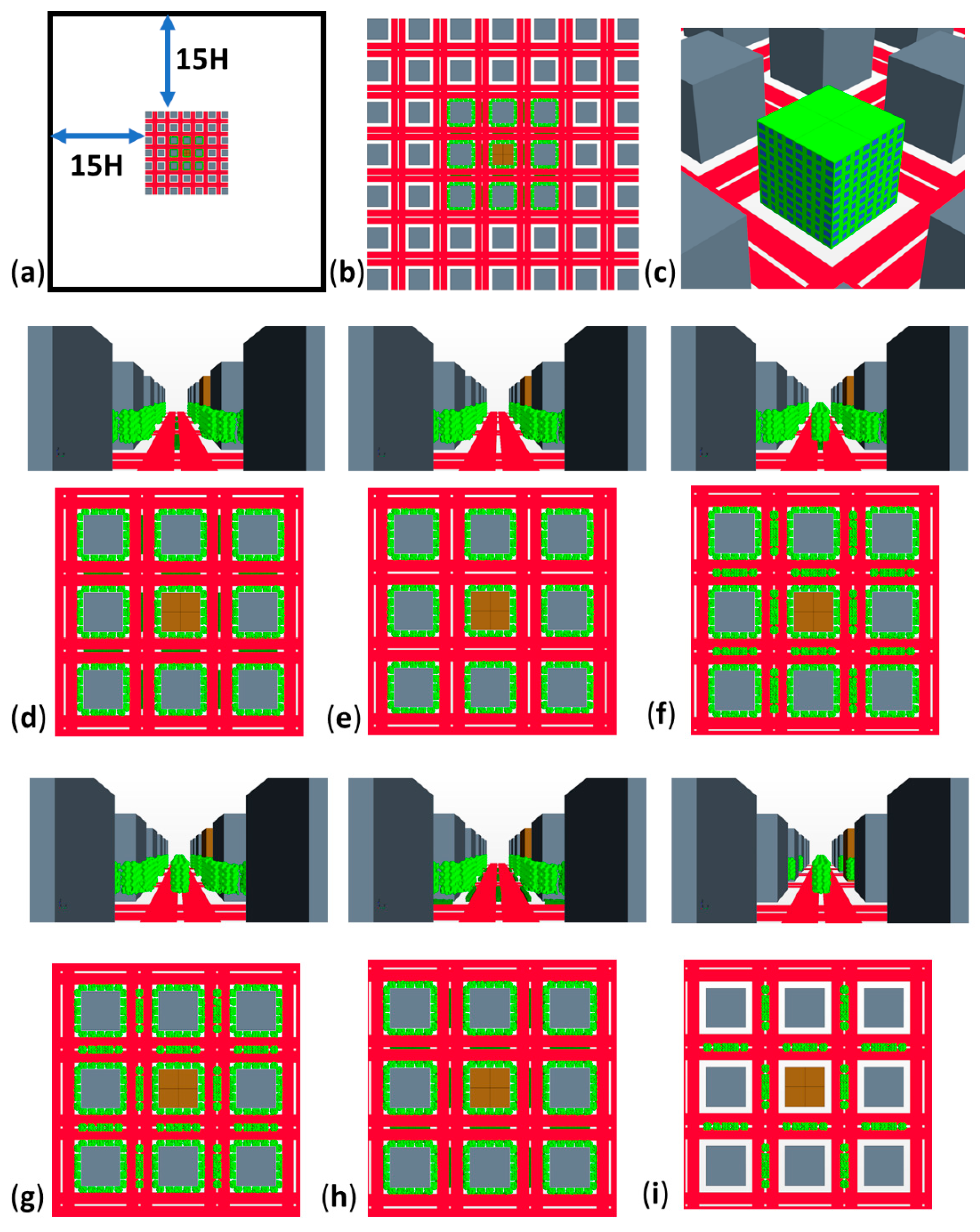
2.1. Description of Urban Geometry and GI Scenarios

CFD modelling is used to assess the impact of different GI scenarios on air quality in an urban environment of high-rise buildings separated by avenues. This approach allows for the investigation of a wide set of vegetation configurations, analyzing deposition and aerodynamic effects, and the effectiveness of the layout of each GI element (street trees, hedgerows, green walls and green roofs) to reduce air pollution.

The urban environment studied is composed by an array of 7 × 7 buildings (Figure 1). Building height (H) is 35 m and the ratio between the building height and street width (W) is 1. The dimensions of the urban area simulated are 455 m × 455 m and the ratio of plan built area occupied by buildings to the total area under consideration (packing density) is 0.25. This is an idealized urban configuration of high-rise buildings separated by avenues resembling a real neighborhood (e.g., the packing density is within the range of planar area indexes that typically occur in urban areas) [52]. Different types of GI composed by different combinations of street trees and hedgerows in the sidewalks and in the middle of the avenues (median strip) are implemented in the central area of the neighborhood (Figure 1,

Table 1. Description of the 19 GI scenarios investigated.

Scenario	Sidewalk GI	Median Strip GI	Green Roof and Green Walls
BASE	NO	NO	NO
BASE_GRGW	NO	NO	YES
VEG_1	15 m height trees	Hedgerows	NO
VEG_1_T10 m	10 m height trees	Hedgerows	NO
VEG_1_GRGW	15 m height trees	Hedgerows	YES
VEG_2	15 m height trees	NO	NO
VEG_2_T10 m	10 m height trees	NO	NO
VEG_2_GRGW	15 m height trees	NO	YES
VEG_3	15 m height trees	15 m height trees + hedgerows	NO
VEG_3_T10 m	10 m height trees	10 m height trees + hedgerows	NO
VEG_3_GRGW	15 m height trees	15 m height trees + hedgerows	YES
VEG_4	15 m height trees	15 m height trees	NO
VEG_4_T10 m	10 m height trees	10 m height trees	NO
VEG_4_GRGW	15 m height trees	15 m height trees	YES
VEG_5	15 m height trees + hedgerows	Hedgerows	NO
VEG_5_T10 m	10 m height trees + hedgerows	Hedgerows	NO
VEG_5_GRGW	15 m height trees + hedgerows	Hedgerows	YES
VEG_6	NO	15 m height trees	NO
VEG_6_T10 m	NO	10 m height trees	NO
VEG_6_GRGW	NO	15 m height trees	YES

). Besides the effects of the different GI scenarios on the pollutant emitted in the study area with vegetation, this allows for the investigation of the barrier effect on pollutants emitted outside the area. In addition, scenarios with green walls and green roofs are also studied. Nineteen different GI scenarios are simulated for 2 wind directions (0° and 45°). To estimate their impact on air quality, the results of these scenarios are compared with those obtained for the BASE cases where GI is not implemented. Tall trees with two different heights are studied (15 m and 10 m). The sizes of crowns are defined, considering some of the real limitations of planting trees in streets (separation with façade, separation between trunks, no invasion of the road, etc.). The studied crowns cover from 4 m height to 15 m height or to 10 m height, depending on the tree height. The horizontal diameter of the crown is 6 m. Trees are located in a row in the sidewalks and/or in the median strip, with a separation between trunks of 8 m. In addition, there is a separation between crowns and building walls of 0.5 m. A leaf area density (LAD) of 0.5 m² m⁻³ is considered (LAI = 7.5 and 5), where LAD and LAI are defined as the leaf area per unit volume or per unit projection area on the ground, respectively. Those values are within the range of typical LAD of urban trees [27,28]. Hedgerows are 1.5 m height and 2 m width when they are in the median strip. However, for hedgerows placed in the sidewalks, their widths are 1.5 m to save space for pedestrians. LAD of hedgerows is 4 m² m⁻³ [27,32]. Green walls are implemented in the central building of the neighborhood on the surface of the façade without windows, and a green roof on the roof surface of this building (Figure 1c). The aerodynamic effects of green walls and green roofs are neglected, and deposition is estimated considering a leaf area index (LAI) of 1 [48,53].

2.2. CFD Modelling Set-Up

CFD simulations are based on Reynolds-averaged Navier–Stokes equations with realizable k-ε turbulence model, where k is the turbulent kinetic energy and ε is the dissipation rate of turbulent kinetic energy. The equations are solved with the commercial software STAR-CCM+ version 15.04.010 [54]. Pollutant is considered non-reactive, and its dispersion is simulated by means of a transport equation of a passive scalar with a Schmidt number of 0.3 [40,41]. In the present study, only traffic emissions are considered, which are homogeneously distributed along the streets where two roads with three lanes are modelled (in red in Figure 1). Since the objective is to investigate traffic-related pollutants, results can be extrapolated to nitrogen oxides (NO_x) or particulate matter (PM). However, some characteristics of the pollutant should be considered, for instance, that the deposition is greater for PM than for NOx. Aerodynamic effects of GI are modelled through a sink term in the momentum equations (S_ui, Equation (1)) and sink/source terms in the turbulence equations for k (S_k, Equation (2)) and for ε (S_ε, Equation (3)) proportional to LAD [28].

These terms are defined as:

$$S{u}_i=-\rho LAD{c}_{d}U{u}_i,$$

(1)

$$S_k=\rho LAD{c}_d\left({\beta }_p{U}^3-{\beta }_{d}Uk\right),$$

(2)

$$S_{\epsilon }=\rho LAD{c}_d\left(C_{\epsilon 4}{\beta }_p\frac{ϵ}{k}{U}^3-C_{\epsilon 5}{\beta }_{d}U\epsilon \right),$$

(3)

where ρ is the air density, c_d is the sectional drag coefficient for vegetation (0.2), U is the wind speed, and u_i is the velocity component in direction i, β_p is the fraction of mean kinetic energy converted into turbulent kinetic energy, β_d is the dimensionless coefficient for the short-circuiting of turbulent cascade, and C_ε4 and C_ε5 are model constant. β_d, C_ε4 and C_ε5 are computed based on analytical expressions of [55] with β_p = [19,41,56]:

$${\beta }_d=C_{\mu }^{0.5}{\left(\frac{2}{\alpha }\right)}^{\frac{2}{3}}{\beta }_p+\frac{3}{{\sigma }_k},$$

(4)

$$C_{\epsilon 4}\left(=C_{\epsilon 5}\right)={\sigma }_k\left(\frac{2}{{\sigma }_{\epsilon }}-\frac{C_{\mu }^{0.5}}{6}{\left(\frac{2}{\alpha }\right)}^{\frac{2}{3}}\left(C_{\epsilon 2}-C_{\epsilon 1}\right)\right),$$

(5)

where C_ε4 = C_ε5 and α, C_µ, σ_k, σ_ε, C_ε1, C_ε2 are 0.05, 0.09, 1, 1.3, 1.44, 1.92.

The dry deposition of pollutant to vegetation is modelled by means of a mass sink in the transport equation (S_d, Equation (6)) proportional to LAD, deposition velocity (V_dep), and concentration of pollutant (C(x,y,z)) at location of vegetation (x,y,z).

$$S_d=-LAD V_{dep}C\left(x,y,z\right),$$

(6)

To investigate the relative contribution of aerodynamic and deposition effects, GI scenarios are simulated for three different depositions (V_dep = 0, 0.01 and 0.05 m s⁻¹). Deposition velocity depends on the type of pollutant and vegetation. Larger values are for PM deposition. Many discrepancies between published values of deposition velocity were found and the deposition velocities used in the present study are within the range of these values [28]. The same approach for modelling the vegetation was successfully used by [19,32,40,41,56] and it is also similar to those employed by [23,34,38].

The height of the computational domain is 11 H and the distance between lateral boundaries and the building array is 15 H, which is in accordance with the best practice guidelines of COST Action 732 [57,58]. Buildings and ground are modelled as wall, although the roughness for building surfaces is neglected whereas for the ground is z₀ = 0.03 m. This value is selected considering the relationship between equivalent sand-grain roughness and aerodynamic roughness length and the first cell height close to ground and wall limitation [59]. Zero normal velocity and zero normal gradients of all variables (symmetry conditions) are imposed at the top of domain. At inlet boundaries, neutral profiles of velocity, turbulent kinetic energy, and ε are established [60] (Equations (7)–(9)).

$$u\left(z\right)=\frac{u_{*}}{\kappa }\ln \left(\frac{z+z_0}{z_0}\right),$$

(7)

$$k=\frac{u_{*}^2}{\sqrt{C_{\mu }}},$$

(8)

$$\epsilon =\frac{u_{*}^3}{\kappa \left(z+z_0\right)},$$

(9)

where u* is the friction velocity and κ is von Karman’s constant (0.4). These profiles are widely used in CFD simulation over urban environments [15,40,61]. Friction velocity is set as u* = 0.22 m s⁻¹, so inlet wind speed at 10 m is 3.2 m s⁻¹, which is similar to inlet wind speed used in other studies over real urban environment [40,62,63]. The pollutant concentration at the inlet boundaries is considered as zero and only traffic emissions in the numerical domain are considered.

The numerical domain is discretized using an irregular polyhedral mesh with hexahedral cells close to the obstacles, emissions, and ground. Inside the building array, the size of polyhedral cells is around 2.5 m with refinements around buildings and emission area and two prism layers of 0.5 m around these surfaces. A grid sensitivity test is performed to select an appropriate mesh for running the set of simulations (114 simulations in total). Three different grid resolutions are used to simulate the BASE scenario for 0° wind direction. The surfaces of the central building and the emission area are meshed with refinements of about 0.75 m, 0.5 m, and 0.25 m for the coarse, medium, and fine grids, respectively. The growth rate of cell size from these refinements is 1.05. The total number of cells is 8.3 × 10⁶, 11.5 × 10⁶, and 30.7 × 10⁶ for the coarse, medium, and fine meshes, respectively. Streamwise velocity (U), vertical velocity (W), and turbulent kinetic energy (k) for the three grids are compared at different vertical profiles around the central building. The results obtained are very similar, being the flow around the buildings similar for the three meshes (Figure S2 in Supplementary Material). The medium grid is therefore selected as a good compromise between accuracy and computational cost.

Flow around the buildings for the BASE scenario is validated by using data from wind-tunnel [64], which has been previously used to assess CFD simulation performance (e.g., [18,65,66]). Streamwise velocity, vertical velocity, and turbulent kinetic energy are evaluated at different vertical profiles (heights below 1.5 H) located in the middle of the central row of buildings (Section S2 in Supplementary Material). For this comparison, these variables are normalized by using streamwise velocity and turbulent kinetic energy at 3 H. Statistical metrics such as fractional bias (FB), the normalized mean-square error (NMSE), the fraction of prediction that are within a factor of two of the observation (FAC2), and the correlation coefficient (R) are computed. Their values indicate a general good model performance with a slight underestimation of turbulent kinetic energy (Table S1 in the Supplementary Material). All statistical metrics fall within the ranges proposed by [67] for urban environments and the more restricted intervals proposed by [68], except for FB for k, which is slightly out of the proposed range. These discrepancies are due to the differences between model set-up and wind-tunnel experiment. The first difference is the size of the building array. The modelled array has 7 rows of buildings, while the array corresponding to the wind-tunnel experiment has 11 rows. The limit of the array can induce a slight influence on the results in the central row of buildings, and it is different depending on the size of the array. In the present case, the array is wide enough to these differences are small, but they could be still visible. The second difference is due to the fact that the inlet profiles of wind speed and turbulent kinetic energy are slightly different between the model (Equations (1)–(3)) and the experiments. In the wind-tunnel experiment, the mean streamwise velocity followed a power-law profile and the experimental turbulent kinetic energy profile was developed in the wind tunnel. Hence, these profiles are slightly different from the neutral inlet profiles of wind speed and turbulent kinetic energy (Equations (1) and (2)) imposed in CFD simulations. The normalized results minimize the differences between variables; however, this small influence can be still visible. Vegetation modelling cannot be evaluated for the same GI scenarios studied in the present paper since experimental data are not available for these configurations. However, the same vegetation modelling approach was applied in several urban environments both in simplified and real configurations and validated in previous studies [32,40,41,56]. Pollutant concentrations (NO_x, NO₂, PM₁₀) were also appropriately modelled in real environments with urban GI that used the same vegetation model to simulate the effects of trees on air quality [15,19,24,62]. More details about validation are provided in the Supplementary Material of the paper (Section S2 in the Supplementary Material).

The methodology to assess the impact of GI scenarios on air quality consists of the comparison of pollutant concentrations obtained for these types of GI with the concentrations for the BASE scenarios, considering similar meteorological conditions. Likewise, the effects of varying the characteristics of GI elements are evaluated comparing different GI scenarios. Since the study is focused on population exposure, pollutant concentrations are evaluated at pedestrian level (3 m height). A height of 3 m is selected because it is the height of the intake systems of the air quality monitoring stations to measure pollutant concentrations employed for air quality assessment. Other similar studies used the same height [15,40,41,62]. The distribution of concentrations and spatially averaged concentrations in a horizontal section at this height are used to assess the impacts of multiple GI scenarios at different areas covering: (1) the whole area where GI is implanted (Neighborhood), (2) only sidewalks and crosswalks of the neighborhood (Sidewalks), and (3) only the sidewalk around the central building (Building). To provide the results in a more generalizable way to compare scenarios, the modelled concentration is normalized as follow:

$$C_{norm}\left(x,y,z\right)=\frac{C\left(x,y,z\right)u_{*}}{Q},$$

(10)

where Q is the source emission rate of traffic-related pollutant in kg m⁻² s⁻¹.

3. Results

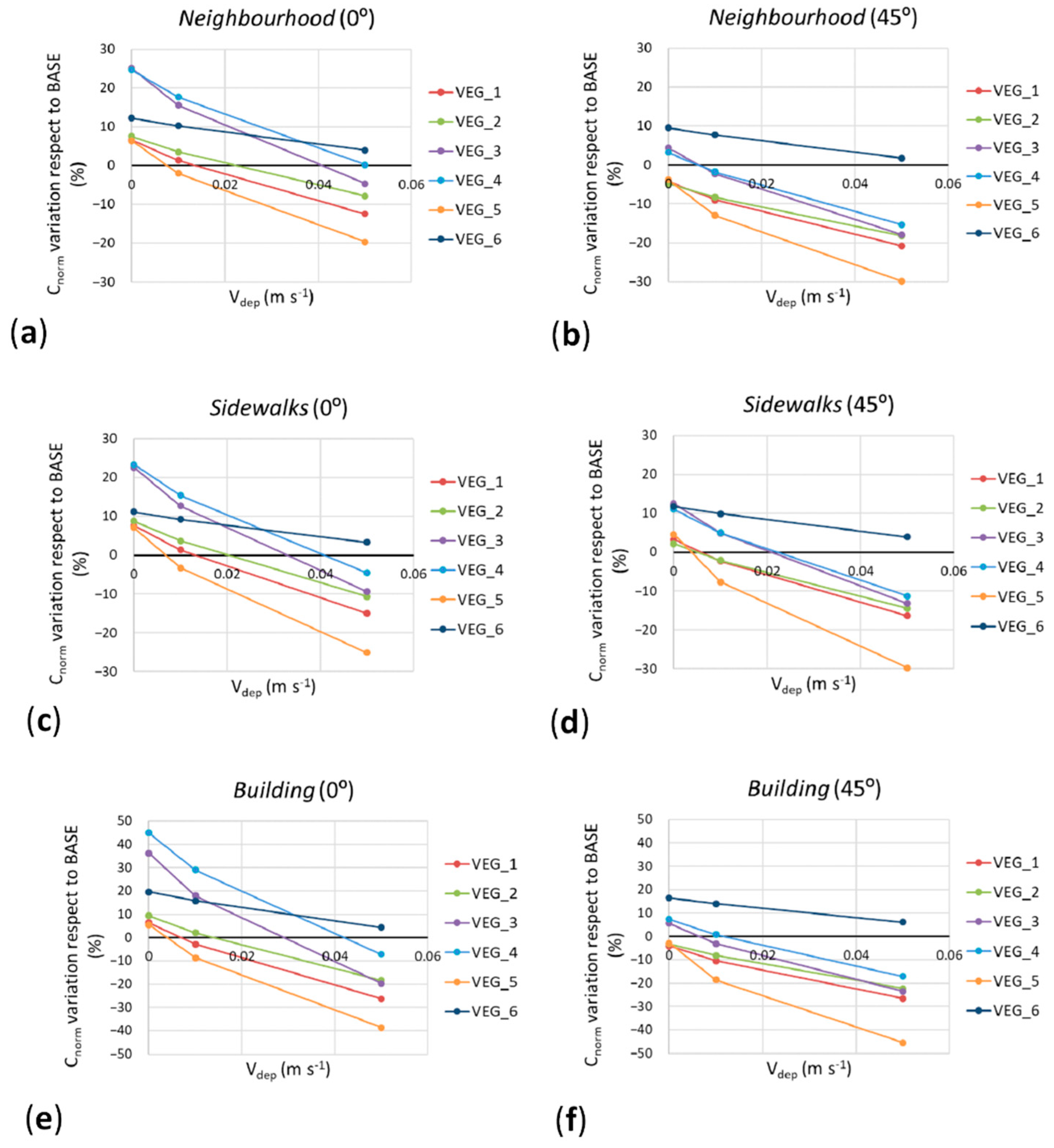
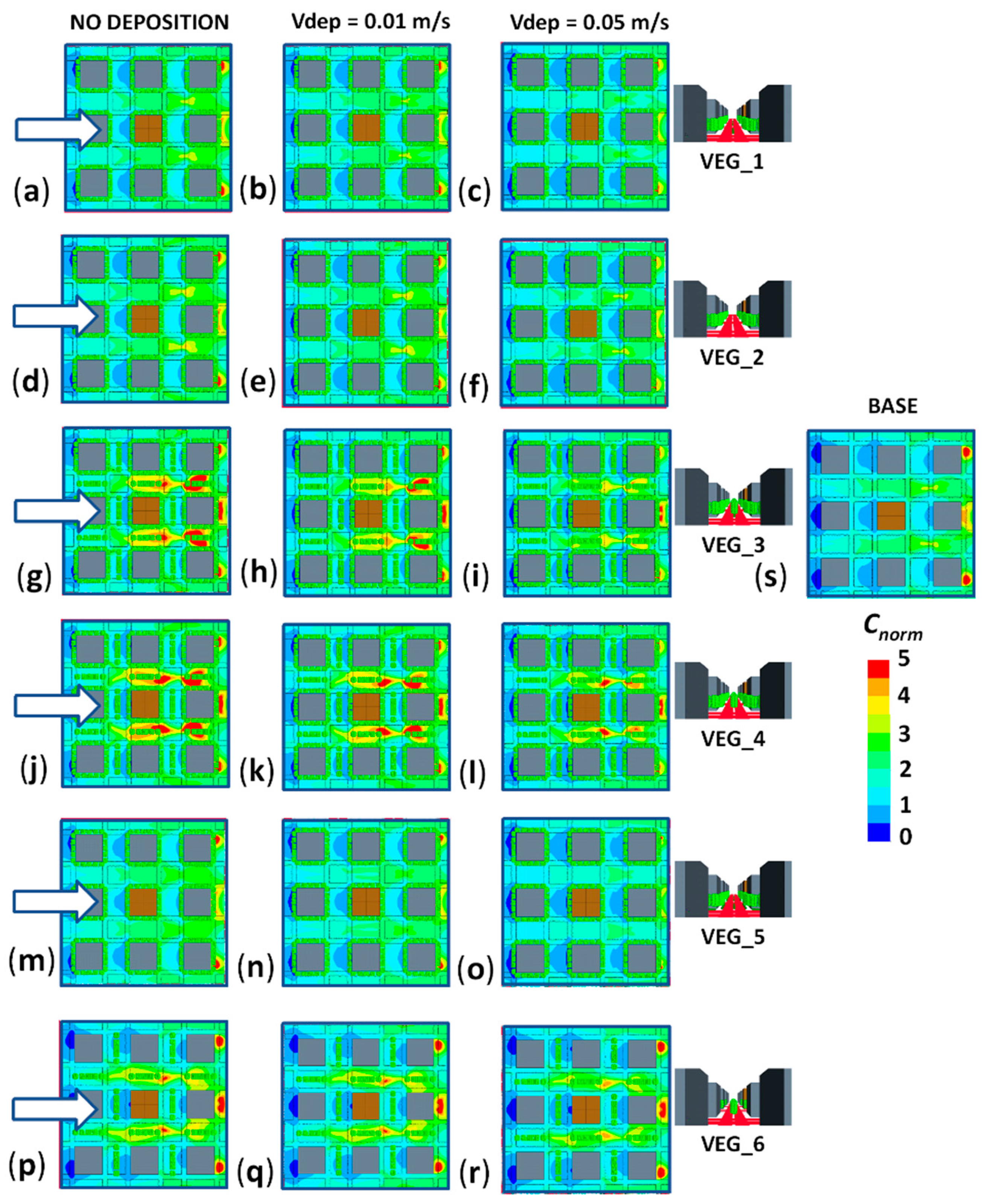
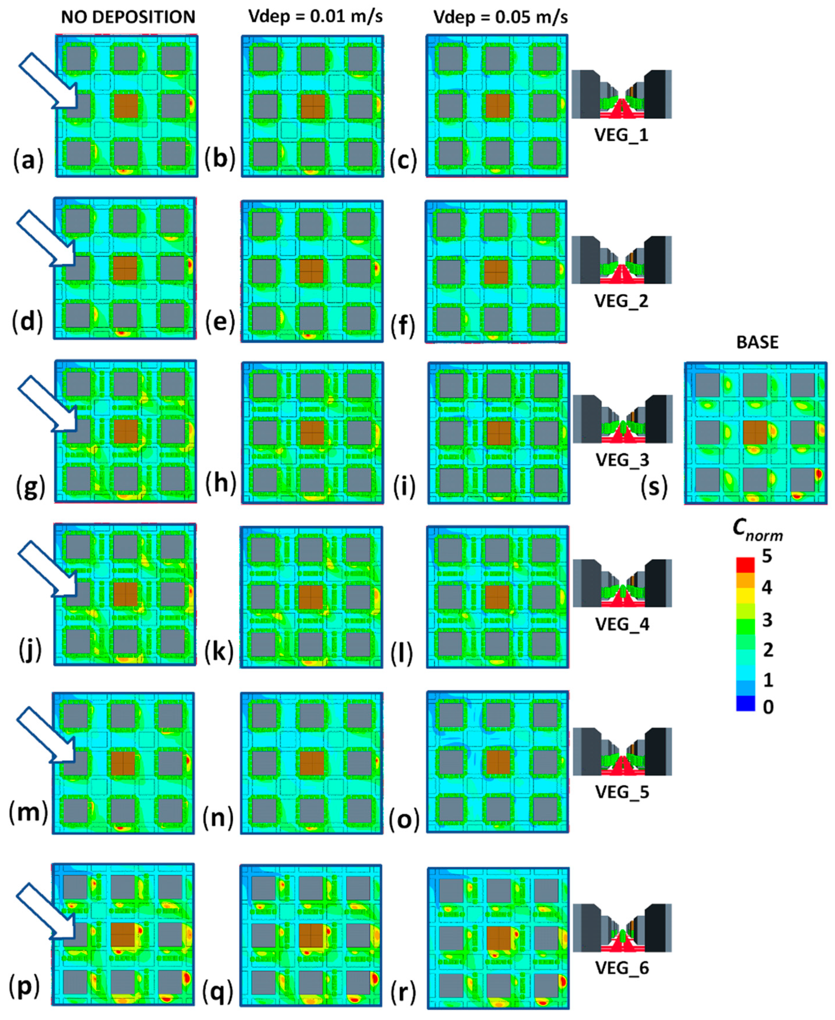
3.1. Impact of Location of GI Elements: Aerodynamic and Deposition Effects

Firstly, the effects of the GI scenarios on the concentration of a traffic-related pollutant (e.g., NO_x, PM10) at pedestrian level are investigated. The spatially averaged concentrations in a horizontal section at 3 m are computed for each GI scenario to assess these impacts at the areas described previously covering different extension of the domain (Neighborhood, Sidewalks and Building).

Table 2. Spatially averaged C_norm for the BASE case for both wind directions.

Wind Direction (°)	Neighborhood	Sidewalks	Building
0	1.65	1.56	1.40
45	1.84	1.73	1.99

shows the spatial-average concentrations for the BASE case for both wind directions (0° and 45°). As it can be seen, the spatially averaged concentrations are larger for the 45° wind direction. To investigate the contribution of deposition and aerodynamic effects on concentrations for each scenario, the relative variation of spatial-average C_norm compared to BASE case, considering different deposition velocities, is represented in Figure 2. In addition, it should be considered that concentrations depend on wind direction.

Concentrations in the study area (zone with GI implemented) depends not only on the pollutant emissions in that zone but also on the pollutants emitted outside arriving to this area due to wind flow. Then, the general effects of the GI implemented in this area are:

(1)

Reducing the ventilation of the streets in this area.

(2)

Acting as a barrier for the pollutant emitted outside.

(3)

Removing pollutant from air by means of deposition.

Figure 2 shows that the spatially averaged concentrations for VEG_3, VEG_4 and VEG_6 scenarios are larger than those obtained for the other scenarios (VEG_1, VEG_2 and VEG_5). This is due to the former scenarios (VEG_3, VEG_4 and VEG_6) having trees in the median strip, which weaken the street ventilation (especially for the 0° wind direction), increasing the average concentrations.

Focusing only on the aerodynamic effects (cases with V_dep = 0), for the 0° wind direction, larger spatially averaged concentrations are observed for all scenarios other than for the BASE scenario. Then, for this wind direction, the effects of reducing street ventilation in the central area of the domain for all the GI configurations are greater than the barrier effects for the pollutant emitted outside. For the 45° wind direction, the situation is slightly different. In general, the aerodynamic effects are less important than for the 0° wind direction. The Neighborhood and Building spatially averaged concentrations for VEG_1, VEG_2, and VEG_5 are slightly lower compared with the BASE scenario. This is due to the barrier effect induced by the trees in sidewalks for the pollutant emitted outside the central area. For both wind directions, spatially averaged concentrations for VEG_1, VEG_2, and VEG_5, all of them with trees at the sidewalks, are similar, indicating that the aerodynamic effects of these GI are also similar. Therefore, the street ventilation is not affected by the hedgerows in the median strip (VEG_1) and in the sidewalks (VEG_5). This is due to the fact that the size of hedgerows is small in comparison with the size of the streets. To study the effects of trees in the sidewalks for the GI scenarios with trees in the median strip, the spatially averaged concentrations for VEG_3, VEG_4, and VEG_6 scenarios are compared. The spatially averaged concentrations for VEG_6 are found to be lower than for VEG_3 and VEG_4, for the 0° wind direction. This fact indicates that adding trees in the sidewalks of VEG_3 and VEG_4 scenarios induce a larger reduction in the ventilation in the area with GI. However, for the 45° wind direction, the Neighborhood and Building spatially averaged concentrations for VEG_6 scenario are larger than those obtained for VEG_3 and VEG_4. For this wind direction, adding trees in the sidewalks to the ones in the median strip (VEG_3 and VEG_4 scenarios) modifies the wind flow in the streets, acting as a barrier for the pollutant emitted outside the central area.

Concentrations for all scenarios decrease as deposition increases. For a deposition velocity of 0.05 m s⁻¹, all scenarios except VEG_6 induce a reduction in spatially averaged concentrations with respect to the BASE scenario. Focusing on concentrations obtained for V_dep = 0.01 m s⁻¹, spatially averaged concentrations over the three areas (Neighborhood, Sidewalks, and Building) for the VEG_5 (and in most of the cases for the VEG_1) scenario are lower than those obtained for the BASE scenario for both wind directions. Pollutants removed from air through deposition depend on the amount of vegetation. The presence of hedgerows decreases concentrations (Figure 2). This fact can be observed comparing spatially averaged concentrations for the VEG_5 and VEG_1 scenarios, and also, concentrations for VEG_3 with those obtained for VEG_4. In the first case, the aerodynamic effects of both GI scenarios are similar, however, the hedgerows in the sidewalks induce a larger deposition for VEG_5 and consequently a more intense decrease of the spatial-average concentrations for this scenario. In the comparison between VEG_3 and VEG_4 scenarios, similar effect of the hedgerows in the median strip is found.

However, the effects of different types of GI in the scenarios investigated are spatially heterogeneous. Figure 3 and Figure 4 show maps of C_norm at 3 m height for all the GI scenarios without deposition and considering deposition with V_dep = 0.01 and 0.05 m s⁻¹. It can be observed that for some scenarios, even the spatially averaged concentration decreases, in some, zone C_norm increases with respect to BASE, and in others, decreases. For instance, this behavior can be found for VEG_3 with V_dep = 0.05 m s⁻¹ for the 0° wind direction. For this scenario, the concentrations in the median strip are larger than those obtained for BASE scenario in that zone. As previously explained, this is due to the reduction in ventilation induced by the trees in the median strip. In addition, it can be observed for 45° scenarios that the sidewalks trees act as a barrier for pollutants emitted outside the study area, reducing the concentrations at the leeward walls of buildings.

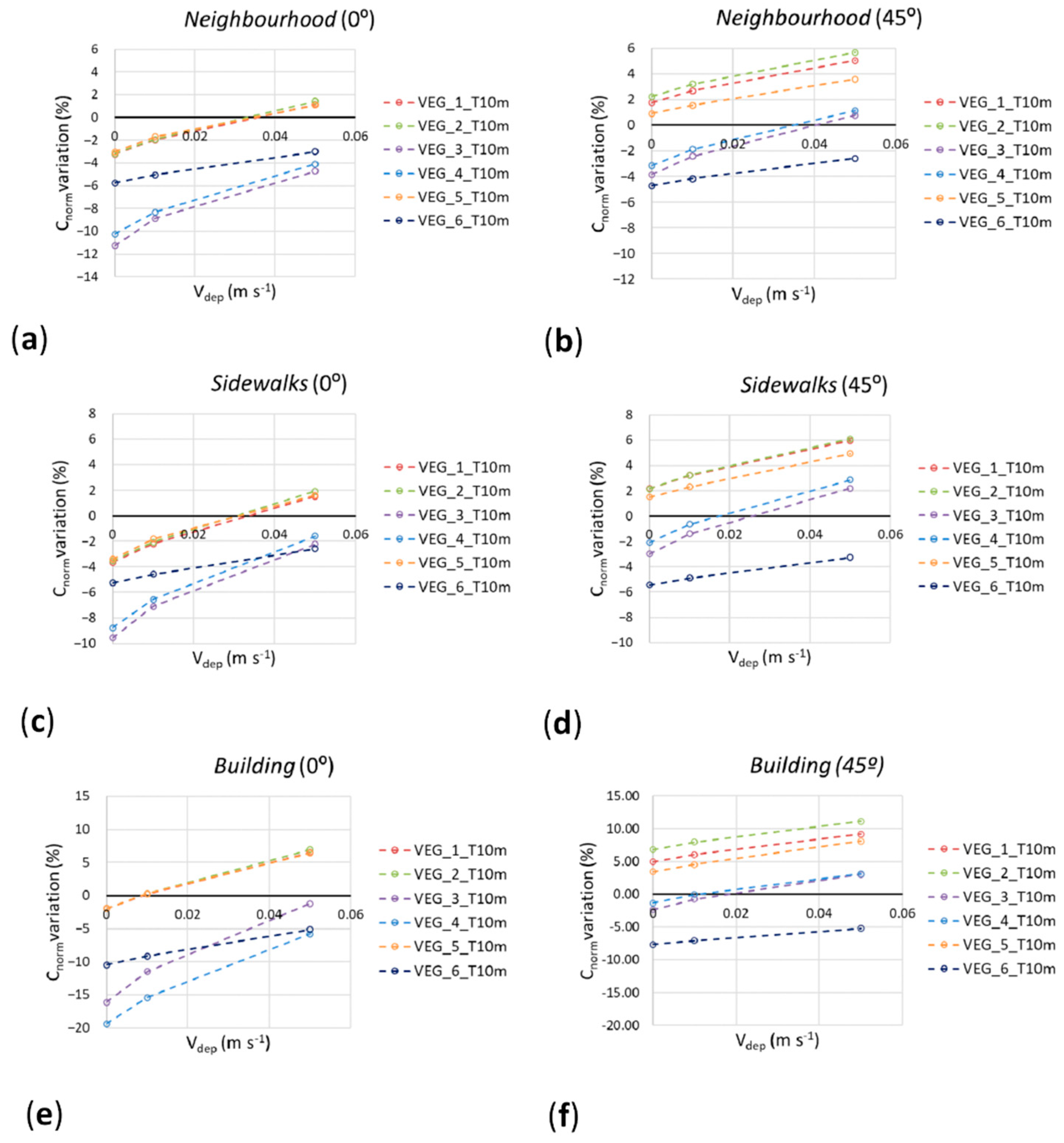
3.2. Impact of the Height of Trees

The impact of the height of trees on traffic-related pollutant concentration is investigated here, comparing GI with 10 m height trees and GI with 15 m height trees.

The spatially averaged concentrations in a horizontal section at 3 m over the three areas (Neighborhood, Sidewalks and Building) are computed for each GI scenario with 10 m height trees. In order to investigate the effects of planting lower-height trees, the variation of these spatially averaged concentrations for GI with 10 m height trees with respect to the same GI scenario with 15 m height trees for both wind directions is studied (Figure 5). Focusing on the aerodynamic effects (no deposition), it can be observed that concentrations for all GIs decrease as the height of trees decreases for the 0° wind direction. This is due to the improvement of the ventilation in the streets as the height of trees decreases. Unlike the 0° wind direction, for the 45° wind direction, spatially averaged concentrations for the GI scenarios without trees in the median strip (VEG_1, VEG_2, and VEG_5) increase as the height of trees decreases. This is due to the decrease in the barrier effects of sidewalk trees, which are more important for these cases, as the height of trees increases from 10 m to 15 m. As the deposition velocity increases (the deposition effects increase), the decrease in concentrations for 10 m height trees scenarios is smaller than for 15 m height trees scenarios, i.e., less quantity of pollutant is removed from air since there is a smaller amount of leaves. Consequently, C_norm for the GI with 10 m height trees is higher than for the GI with 15 m height trees. It can be observed that for the 0° wind direction, the spatially averaged concentrations for GI scenarios with trees in the median strip (VEG_3, VEG_4, and VEG_6) are lower for 10 m height trees since the reduction in ventilation is the most important contribution for these GI scenarios. For the 45° wind direction, the spatially averaged concentrations for GI scenarios without trees in the median strip (VEG_1, VEG_2, and VEG_5) are larger for 10 m height trees since the effect of the barrier induced by sidewalks trees is the most important contribution.

The effects of planting lower trees are: (1) a general improvement of the ventilation in the streets of the central part of the neighborhood; (2) a reduction in the barrier effect of GI with respect to the pollutant emitted outside the zone with GI; and (3) a decrease in pollutant deposition due to the decrease in the amount of vegetation. The first point induces a general reduction in concentrations, but the other two effects induce an increase in concentrations.

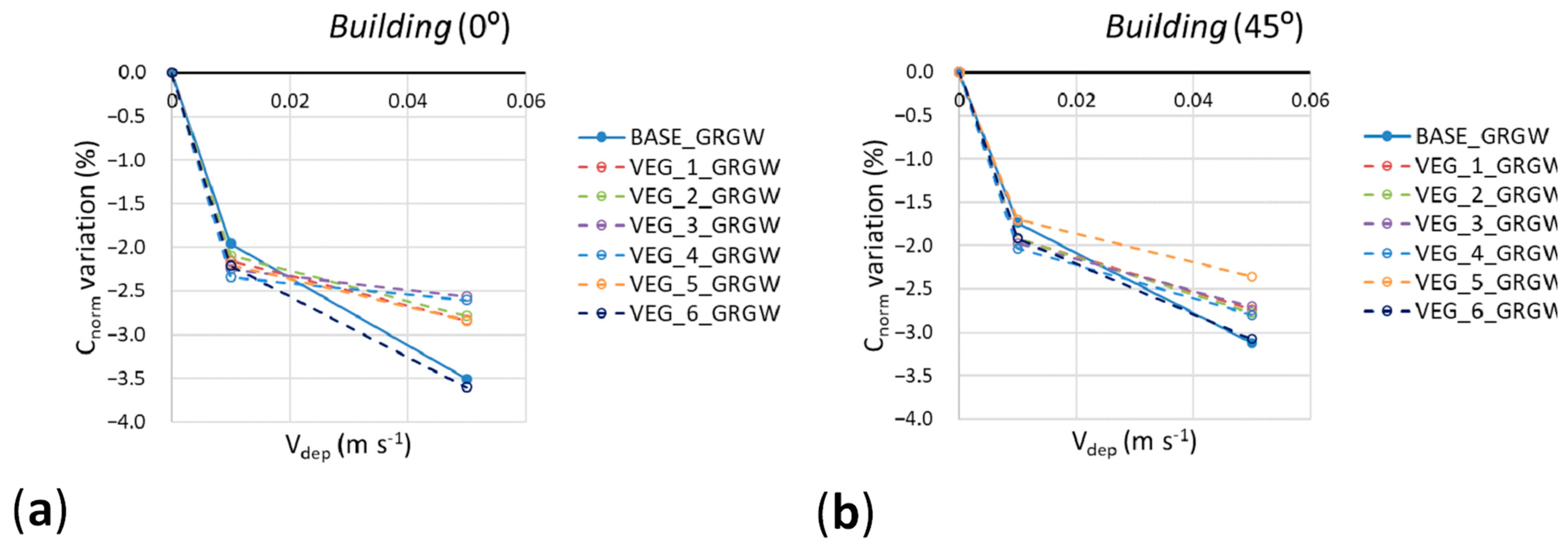
3.3. Impact of Green Walls and Green Roofs

Green walls and green roof are implemented in the central building and their impact is spatially limited. Variations of spatially averaged concentrations over Neighborhood and over Sidewalks for GI with and without green walls and green roof are negligible. Their impacts can be only found over the sidewalk around the central building (Building). However, the differences between scenarios are lower than 4% (Figure 6).

4. Discussion and Conclusions

This paper studies the impact of a wide set of GI elements on traffic-related pollutant concentrations at the pedestrian level within an idealized three-dimensional urban area. GI provides different benefits such as social benefits (e.g., making cities more pleasant), economic benefits (e.g., increasing property value), microclimate regulation, health benefits (e.g., psychological values), carbon sequestration, reducing energy use, etc. [28,69,70,71]. Regarding air quality, the results of the present paper indicate, as previous studies (e.g., [27,28]), that using GI alone is ineffective as a general air quality mitigation measure. However, according to the approach, “the right tree (in this case, GI) in the right street”, proposed by Buccolieri et al. [28], our results also show that, selecting appropriate layouts of GI elements, GI can also help to reduce population exposure to air pollution even in a scenario with high buildings such as the study area investigated here. In this paper, it was possible to investigate the relative influence of each GI element due to the large number of simulated scenarios performed. It is noteworthy that the recommendations proposed for improving air quality should be considered not only to solve urban air pollution problems, but also when GI is designed for other purposes (e.g., improving urban climate). GI design should be addressed to obtain a trade-off solution between the different ecosystem services and disservices provided.

Regarding the trees in the streets, this study indicates that, for almost all the cases, the aerodynamic effects produce an increase in concentrations. Therefore, the general population exposure to traffic-related pollutants also increases. This agrees with previous studies (e.g., [12,23,27,34,35,36,37]). Indeed, Kumar et al. [47] recommends no trees for street canyons with aspect ratios H/W < 2 and no forms of vegetation except green walls for deep street canyons (H/W > 0.5). In the current study, the aspect ratio of the streets is H/W = 1, however the building packing density is 0.25, so the length of streets is not very long. For this three-dimensional configuration, the present study shows the importance of the location of trees and how street trees in the right locations can reduce pollutant concentrations at street level considering pollutant depositions. Trees in the median strip are found to be in an adverse location. These trees produce an increase in the spatially averaged concentrations, in particular for the 0° wind direction. Focusing on local concentrations, the larger increases in concentrations are found in streets parallel to the wind, due to a drastic reduction in ventilation there, and as a consequence, traffic-related pollutant are retained in that area. This fact agrees with [39] where, for parallel winds, the concentration was found higher for an isolated street canyon with trees. In streets perpendicular to wind direction, this effect is not so important, as even for some scenarios with deposition, there are concentration decreases in these areas. On the contrary, the presence of trees in the sidewalks is found as a right location. These trees are especially good acting as a barrier for the pollutant emitted outside of the zone with implemented GI, in particular for the 45° wind direction. Therefore, this fact suggests that GI implementation combined with measures of traffic-emission reductions in the area with GI will produce the best performance to improve air quality. However, further studies about the combination of air pollution mitigation strategies should be investigated in the future. Regarding the influence of the height of trees, the decrease in height induces a decrease in deposition and aerodynamic effects. Therefore, the general impact of changing the height of trees on pedestrian-level concentrations depends on what effect is more important for each GI configuration.

The results of the present paper indicate that for this configuration, the street ventilation is not affected by the hedgerows in both locations. Gromke and Blocken [23] determined the crown volume fraction as key parameter on the effects of trees on pollutant concentration. It was defined as the volume occupied by tree crowns within a street canyon section. In this case, the hedge volume fraction can be defined in a similar way, using hedgerow volume fraction. In the present study, this parameter is very small for hedgerows since buildings are tall and the width of streets large (H/W = 1). Therefore, for this urban configuration, the presence of hedgerows is positive for air quality due to pollutant deposition effects, and higher the deposition velocity, the more important air quality improvements are. This agrees with [27], that establishing the performance of hedgerows for improving air quality is dominated by their ability to remove from the air pollutants emitted by local sources.

Finally, the effects of green walls and green roof on spatially averaged concentrations are found to be limited to areas around the building where both measures are implemented. In addition, the reduction in concentrations is not large, and the effects of trees and hedgerows are found to be more important. Previous studies (e.g., [48,49]) estimated different pollutant concentrations reduction in a street canyon depending on street canyon geometry, and LAI. Qin et al. [49] observed that larger H/W lower concentration reductions. The reductions obtained in the present study are lower than those, which is explained by the fact that the street ventilation in this configuration is higher than in a street canyon. Therefore, the residence time of pollutants close to green walls is lower and, consequently, the deposition is also lower. However, it is noteworthy that the effects of green walls and green roof are always positive in terms of air quality since they do not reduce the street ventilation and provide other benefits like the improvement of building energy consumption. Therefore, as proposed Kumar et al. [47], they could be a good option for deep street canyons.

This paper is based on numerical simulations using a previously validated CFD model and it focuses on an idealized urban configuration of high-rise buildings. This configuration is representative of some areas of certain cities with a regular layout of buildings. Results obtained in this study can be extrapolated to urban environment of high-rise buildings separated by avenues with aspect ratios around 1 and packing densities around 0.25. In general, the real layout of a city is much more complex that the one used in this paper. There, wind flow and pollutant dispersion are also more complex, and particular studies for each real neighborhood are needed to investigate GI effects in detail. However, the results of the present study can help to improve the understanding of their effects, and can be extrapolated for certain areas of complex configurations with similar aspect ratios and packing densities. The impact of GI for more layouts of buildings should be addressed in future studies.

This paper focuses on pollutants emitted by traffic, which is the main source of pollutants in urban areas. However, GI also has an impact on pollution from other distant sources (e.g., industrial emissions). Specifically, GI can capture part of this pollution by means of deposition-decreasing pollutant concentration in the air. In addition, GI can contribute to prevent those pollutants reaching the streets. Aerodynamic and deposition effects are considered in the numerical simulations. The biochemical effects of different vegetation on different pollutants (e.g., the absorption of certain pollutant gases) are not explicitly modelled. However, these effects are included in the value of deposition velocity. The purpose of this study is not to model specific species of trees, hedgerows and green walls/roofs, and typical values of deposition velocities are used. Deposition velocities depend on the type of pollutant and plant species. To provide more information about this issue and the range of deposition effects, different deposition velocities have been investigated. In addition, typical values of LAD and Cd are also used. The canopy of different plants is also different; however, in this study, crowns with regular shape are simulated to consider “standard” trees. The impact of location and layout of vegetation elements is expected to be greater than the effects of the shape of crown (considering the same quantity of vegetation), although those effects should be investigated in future studies. Furthermore, the cost–benefit of vegetation at species level should be considered for an appropriate plant selection for urban air quality management [33], not only with regards to the pollutant removal capacity, but also other factors, such as emissions of pollen or biogenic volatile organic compounds and air pollution tolerance [12]. In addition, it is necessary to understand the suitability of each considered plant species to the environmental conditions of the intended planting location [33].

Finally, it should be noted that this study is focused on the impact on air quality, and the transpiration effects of plants are not considered. However, these effects can lead to an increase in local humidity, which can further affect air pollutant such as hygroscopic growth and particle transformation. Deposition and aerodynamic effects of GI and the impact of location and layout of vegetation elements studied in this paper are expected to be greater than those effects. However, they should be addressed in future studies, specifically using field experiments, to obtain data to appropriately model these processes in CFD simulations, which is still a challenge.

In general, future studies should address the need to perform more field experiments to complement modelling data and help to improve simulations modelling other processes. Future studies should focus on the design of GI from a holistic point of view that consider the different services and disservices (air pollutant removal, improving urban climate, etc.).

References

1. World Health Organization (WHO). Ambient (Outdoor) Air Quality and Health. Fact Sheet, Updated May 2018. Available online: https://www.who.int/news-room/fact-sheets/detail/ambient-(outdoor)-air-quality-and-health (accessed on 26 June 2022).
2. European Environment Agency (EEA). Air Quality in Europe—2020 Report; EEA Report No 09/2020 1977–8449; European Environment Agency: Copenhagen, Denmark, 2020.
3. Boogaard, H.; Janssen, N.A.; Fischer, P.H.; Kos, G.P.; Weijers, E.P.; Cassee, F.R.; van der Zee, S.C.; de Hartog, J.J.; Meliefste, K.; Wang, M.; et al. Impact of low emission zones and local traffic policies on ambient air pollution concentrations. Sci. Total Environ. 2012, 435, 132–140. [Google Scholar] [CrossRef]
4. Holman, C.; Harrison, R.; Querol, X. Review of the efficacy of low emission zones to improve urban air quality in European cities. Atmos. Environ. 2015, 111, 161–169. [Google Scholar] [CrossRef]
5. Huang, Y.; Lei, C.; Liu, C.H.; Perez, P.; Forehead, H.; Kong, S.; Zhou, J.L. A review of strategies for mitigating roadside air pollution in urban street canyons. Environ. Pollut. 2021, 280, 116971. [Google Scholar] [CrossRef] [PubMed]
6. Santiago, J.L.; Sanchez, B.; Rivas, E.; Vivanco, M.G.; Theobald, M.R.; Garrido, J.L.; Gil, V.; Martilli, A.; Rodríguez-Sánchez, A.; Buccolieri, R.; et al. High spatial resolution assessment of the effect of the Spanish National Air Pollution Control Programme on street-level NO2 concentrations in three neighborhoods of Madrid (Spain) using mesoscale and CFD modelling. Atmosphere 2022, 13, 248. [Google Scholar] [CrossRef]
7. Gallagher, J.; Baldauf, R.; Fuller, C.H.; Kumar, P.; Gill, L.W.; McNabola, A. Passive methods for improving air quality in the built environment: A review of porous and solid barriers. Atmos. Environ. 2015, 120, 61–70. [Google Scholar] [CrossRef]
8. Li, Z.; Ming, T.; Shi, T.; Zhang, H.; Wen, C.Y.; Lu, X.; Dong, X.; Wu, Y.; de Richter, R.; Li, W.; et al. Review on pollutant dispersion in urban areas-part B: Local mitigation strategies, optimization framework, and evaluation theory. Build. Environ. 2021, 198, 107890. [Google Scholar] [CrossRef]
9. Buccolieri, R.; Carlo, O.S.; Rivas, E.; Santiago, J.L.; Salizzoni, P.; Siddiqui, M.S. Obstacles influence on existing urban canyon ventilation and air pollutant concentration: A review of potential measures. Build. Environ. 2022, 214, 108905. [Google Scholar] [CrossRef]
10. Fernández-Pampillón, J.; Palacios, M.; Núñez, L.; Pujadas, M.; Sanchez, B.; Santiago, J.L.; Martilli, A. NOx depolluting performance of photocatalytic materials in an urban area–Part I: Monitoring ambient impact. Atmos. Environ. 2021, 251, 118190. [Google Scholar] [CrossRef]
11. Sanchez, B.; Santiago, J.L.; Martilli, A.; Palacios, M.; Núñez, L.; Pujadas, M.; Fernández-Pampillón, J. NOx depolluting performance of photocatalytic materials in an urban area-Part II: Assessment through Computational Fluid Dynamics simulations. Atmos. Environ. 2021, 246, 118091. [Google Scholar] [CrossRef]
12. Tomson, M.; Kumar, P.; Barwise, Y.; Perez, P.; Forehead, H.; French, K.; Morawska, L.; Watts, J.F. Green infrastructure for air quality improvement in street canyons. Environ. Int. 2021, 146, 106288. [Google Scholar] [CrossRef]
13. Vardoulakis, S.; Fisher, B.E.; Pericleous, K.; Gonzalez-Flesca, N. Modelling air quality in street canyons: A review. Atmos. Environ. 2003, 37, 155–182. [Google Scholar] [CrossRef] [Green Version]
14. Borge, R.; Narros, A.; Artíñano, B.; Yagüe, C.; Gómez-Moreno, F.J.; de la Paz, D.; Roman-Cascon, C.; Díaz, E.; Maqueda, G.; Sastre, M.; et al. Assessment of microscale spatio-temporal variation of air pollution at an urban hotspot in Madrid (Spain) through an extensive field campaign. Atmos. Environ. 2016, 140, 432–445. [Google Scholar] [CrossRef]
15. Santiago, J.L.; Borge, R.; Martin, F.; de la Paz, D.; Martilli, A.; Lumbreras, J.; Sanchez, B. Evaluation of a CFD-based approach to estimate pollutant distribution within a real urban canopy by means of passive samplers. Sci. Total Environ. 2017, 576, 46–58. [Google Scholar] [CrossRef] [PubMed]
16. Santiago, J.L.; Borge, R.; Sanchez, B.; Quaassdorff, C.; De La Paz, D.; Martilli, A.; Rivas, E.; Martín, F. Estimates of pedestrian exposure to atmospheric pollution using high-resolution modelling in a real traffic hot-spot. Sci. Total Environ. 2021, 755, 142475. [Google Scholar] [CrossRef]
17. Santiago, J.L.; Rivas, E.; Gamarra, A.R.; Vivanco, M.G.; Buccolieri, R.; Martilli, A.; Lechón, Y.; Martín, F. Estimates of population exposure to atmospheric pollution and health-related externalities in a real city: The impact of spatial resolution on the accuracy of results. Sci. Total Environ. 2022, 819, 152062. [Google Scholar] [CrossRef]
18. Santiago, J.L.; Rivas, E.; Buccolieri, R.; Martilli, A.; Vivanco, M.G.; Borge, R.; Carlo, O.S.; Martín, F. Indoor-outdoor pollutant concentration modelling: A comprehensive urban air quality and exposure assessment. Air Qual. Atmos. Health, 2022; in press. [Google Scholar] [CrossRef]
19. Santiago, J.L.; Martín, F.; Martilli, A. A computational fluid dynamic modelling approach to assess the representativeness of urban monitoring stations. Sci. Total Environ. 2013, 454–455, 61–72. [Google Scholar] [CrossRef] [PubMed]
20. Kracht, O.; Santiago, J.L.; Martin, F.; Piersanti, A.; Cremona, G.; Righini, G.; Gerboles, M. Spatial Representativeness of Air Quality Monitoring Sites—Outcomes of the FAIRMODE/AQUILA Intercomparison Exercise; Publications Office of the European Union: Luxembourg, 2018. [CrossRef]
21. Vardoulakis, S.; Solazzo, E.; Lumbreras, J. Intra-urban and street scale variability of BTEX, NO2 and O3 in Birmingham, UK: Implications for exposure assessment. Atmos. Environ. 2011, 45, 5069–5078. [Google Scholar] [CrossRef]
22. Di Sabatino, S.; Buccolieri, R.; Salizzoni, P. Recent advancements in numerical modelling of flow and dispersion in urban areas: A short review. Int. J. Environ. Pollut. 2013, 52, 172–191. [Google Scholar] [CrossRef]
23. Gromke, C.; Blocken, B. Influence of avenue-trees on air quality at the urban neighborhood scale. Part II: Traffic pollutant concentrations at pedestrian level. Environ. Pollut. 2015, 196, 176–184. [Google Scholar] [CrossRef] [PubMed] [Green Version]
24. Santiago, J.L.; Sanchez, B.; Quaassdorff, C.; de la Paz, D.; Martilli, A.; Martín, F.; Borge, R.; Rivas, E.; Gómez-Moreno, F.J.; Días, E.; et al. Performance evaluation of a multiscale modelling system applied to particulate matter dispersion in a real traffic hot spot in Madrid (Spain). Atmos. Pollut. Res. 2020, 11, 141–155. [Google Scholar] [CrossRef]
25. Salmond, J.A.; Tadaki, M.; Vardoulakis, S.; Arbuthnott, K.; Coutts, A.; Demuzere, M.; Dirks, K.N.; Heaviside, C.; Lim, S.; Macintyre, H.; et al. Health and climate related ecosystem services provided by street trees in the urban environment. Environ. Health. 2016, 15, S36. [Google Scholar] [CrossRef] [PubMed] [Green Version]
26. Santamouris, M.; Ban-Weiss, G.; Osmond, P.; Paolini, R.; Synnefa, A.; Cartalis, C.; Muscio, A.; Zinzi, M.; Morakinyo, T.E.; Ng, E.; et al. Progress in urban greenery mitigation science–assessment methodologies advanced technologies and impact on cities. J. Civ. Eng. Manag. 2018, 24, 638–671. [Google Scholar] [CrossRef] [Green Version]
27. Abhijith, K.V.; Kumar, P.; Gallagher, J.; McNabola, A.; Baldauf, R.; Pilla, F.; Broderick, B.; Di Sabatino, S.; Pulvirenti, B. Air pollution abatement performances of green infrastructure in open road and built-up street canyon environments—A review. Atmos. Environ. 2017, 162, 71–86. [Google Scholar] [CrossRef]
28. Buccolieri, R.; Santiago, J.L.; Rivas, E.; Sanchez, B. Review on urban tree modelling in CFD simulations: Aerodynamic, deposition and thermal effects. Urban For. Urban Green. 2018, 31, 212–220. [Google Scholar] [CrossRef]
29. Santiago, J.L.; Rivas, E. Advances on the Influence of Vegetation and Forest on Urban Air Quality and Thermal Comfort. Forests 2021, 12, 1133. [Google Scholar] [CrossRef]
30. Al-Dabbous, A.N.; Kumar, P. The influence of roadside vegetation barriers on airborne nanoparticles and pedestrians exposure under varying wind conditions. Atmos. Environ. 2014, 90, 113–124. [Google Scholar] [CrossRef] [Green Version]
31. Baldauf, R. Roadside vegetation design characteristics that can improve local, near-road air quality. Transport. Res. Part D Transp. Environ. 2017, 52, 354–361. [Google Scholar] [CrossRef]
32. Santiago, J.L.; Buccolieri, R.; Rivas, E.; Calvete-Sogo, H.; Sanchez, B.; Martilli, A.; Alonso, R.; Elustondo, D.; Santamaría, J.M.; Martin, F. CFD modelling of vegetation barrier effects on the reduction of traffic-related pollutant concentration in an avenue of Pamplona, Spain. Sustain. Cities Soc. 2019, 48, 101559. [Google Scholar] [CrossRef]
33. Barwise, Y.; Kumar, P. Designing vegetation barriers for urban air pollution abatement: A practical review for appropriate plant species selection. NPJ Clim. Atmos. Sci. 2020, 3, 1–19. [Google Scholar] [CrossRef] [Green Version]
34. Vos, P.E.; Maiheu, B.; Vankerkom, J.; Janssen, S. Improving local air quality in cities: To tree or not to tree? Environ. Pollut. 2013, 183, 113–122. [Google Scholar] [CrossRef] [PubMed]
35. Vranckx, S.; Vos, P.; Maiheu, B.; Janssen, S. Impact of trees on pollutant dispersion in street canyons: A numerical study of the annual average effects in Antwerp, Belgium. Sci. Total Environ. 2015, 532, 474–483. [Google Scholar] [CrossRef]
36. Jeanjean, A.P.; Buccolieri, R.; Eddy, J.; Monks, P.S.; Leigh, R.J. Air quality affected by trees in real street canyons: The case of Marylebone neighbourhood in central London. Urban For. Urban Green. 2017, 22, 41–53. [Google Scholar] [CrossRef]
37. Kumar, P.; Druckman, A.; Gallagher, J.; Gatersleben, B.; Allison, S.; Eisenman, T.S.; Hoang, U.; Hama, S.; Tiwari, A.; Sharma, A.; et al. The nexus between air pollution, green infrastructure and human health. Environ. Int. 2019, 133, 105181. [Google Scholar] [CrossRef] [PubMed]
38. Amorim, J.H.; Rodrigues, V.; Tavares, R.; Valente, J.; Borrego, C. CFD modelling of the aerodynamic effect of trees on urban air pollution dispersion. Sci. Total Environ. 2013, 461, 541–551. [Google Scholar] [CrossRef] [PubMed]
39. Abhijith, K.V.; Gokhale, S. Passive control potentials of trees and on-street parked cars in reduction of air pollution exposure in urban street canyons. Environ. Pollut. 2015, 204, 99–108. [Google Scholar] [CrossRef] [PubMed]
40. Santiago, J.L.; Rivas, E.; Sanchez, B.; Buccolieri, R.; Martin, F. The impact of planting trees on NOx concentrations: The case of the Plaza de la Cruz neighborhood in Pamplona (Spain). Atmosphere 2017, 8, 131. [Google Scholar] [CrossRef] [Green Version]
41. Santiago, J.L.; Martilli, A.; Martin, F. On dry deposition modelling of atmospheric pollutants on vegetation at the microscale: Application to the impact of street vegetation on air quality. Bound. Layer Meteorol 2017, 162, 451–474. [Google Scholar] [CrossRef]
42. Santiago, J.L.; Buccolieri, R.; Rivas, E.; Sanchez, B.; Martilli, A.; Gatto, E.; Martín, F. On the impact of trees on ventilation in a real street in Pamplona, Spain. Atmosphere 2019, 10, 697. [Google Scholar] [CrossRef] [Green Version]
43. Xue, F.; Li, X. The impact of roadside trees on traffic released PM10 in urban street canyon: Aerodynamic and deposition effects. Sustain. Cities Soc. 2017, 30, 195–204. [Google Scholar] [CrossRef]
44. Buccolieri, R.; Jeanjean, A.P.R.; Gatto, E.; Leigh, R.J. The impact of trees on street ventilation, NOx and PM2.5 concentrations across heights in Marylebone Rd street canyon, central London. Sustain. Cities Soc. 2018, 41, 227–241. [Google Scholar] [CrossRef]
45. Gromke, C.; Jamarkattel, N.; Ruck, B. Influence of roadside hedgerows on air quality in urban street canyons. Atmos. Environ. 2016, 139, 75–86. [Google Scholar] [CrossRef]
46. Li, X.B.; Lu, Q.C.; Lu, S.J.; He, H.D.; Peng, Z.R.; Gao, Y.; Wang, Z.Y. The impacts of roadside vegetation barriers on the dispersion of gaseous traffic pollution in urban street canyons. Urban For. Urban Green. 2016, 17, 80–91. [Google Scholar] [CrossRef]
47. Kumar, P.; Abhijith, K.V.; Barwise, Y. Implementing Green Infrastructure for Air Pollution Abatement: General Recommendations for Management and Plant Species Selection. Global Centre for Clean Air Research, University of Surrey. 2019. Available online: https://www.iscapeproject.eu/wp-content/uploads/2019/11/Kumar-et-al.-2019_GI-Pollution-Abatement.pdf (accessed on 26 June 2022).
48. Pugh, T.A.; MacKenzie, A.R.; Whyatt, J.D.; Hewitt, C.N. Effectiveness of green infrastructure for improvement of air quality in urban street canyons. Environ. Sci. Technol. 2012, 46, 7692–7699. [Google Scholar] [CrossRef] [Green Version]
49. Qin, H.; Hong, B.; Jiang, R. Are green walls better options than green roofs for mitigating PM10 pollution? CFD simulations in urban street canyons. Sustainability 2018, 10, 2833. [Google Scholar] [CrossRef] [Green Version]
50. Moradpour, M.; Afshin, H.; Farhanieh, B. A numerical study of reactive pollutant dispersion in street canyons with green roofs. Build. Simul. 2018, 11, 125–138. [Google Scholar] [CrossRef]
51. Jeong, N.R.; Han, S.W.; Kim, J.H. Evaluation of Vegetation Configuration Models for Managing Particulate Matter along the Urban Street Environment. Forests 2022, 13, 46. [Google Scholar] [CrossRef]
52. Grimmond, C.S.B.; Oke, T.R. Aerodynamic properties of urban areas derived from analysis of surface form. J. Appl. Meteorol. Clim. 1999, 38, 1262–1292. [Google Scholar] [CrossRef]
53. Joshi, S.V.; Ghosh, S. On the air cleansing efficiency of an extended green wall: A CFD analysis of mechanistic details of transport processes. J. Theor. Biol. 2014, 361, 101–110. [Google Scholar] [CrossRef] [PubMed]
54. Siemens Digital Industries Software. SimCenter STAR-CCM+. 2021. Available online: https://www.plm.automation.siemens.com/global/es/products/simcenter/STAR-CCM.html (accessed on 26 June 2022).
55. Sanz, C. A note on k−ε modeling of vegetation canopy air-flows. Bound. Layer Meteorol. 2003, 108, 191–197. [Google Scholar] [CrossRef]
56. Krayenhoff, E.S.; Santiago, J.L.; Martilli, A.; Christen, A.; Oke, T.R. Parametrization of drag and turbulence for urban neighbourhoods with trees. Bound. Layer Meteorol. 2015, 156, 157–189. [Google Scholar] [CrossRef]
57. Franke, J.; Schlünzen, H.; Carissimo, B. Best Practice Guideline for the CFD Simulation of Flows in the Urban Environment. COST Action 732—Quality Assurance and Improvement of Microscale Meteorological Models; University of Hamburg (Germany), Meteorological Institute: Hamburg, Germany, 2007; ISBN 3-00-018312-4. [Google Scholar]
58. Di Sabatino, S.; Buccolieri, R.; Olesen, H.R.; Ketzel, M.; Berkowicz, R.; Franke, J.; Schatzmann, M.; Schlunzen, K.; Leitl, B.; Britter, R.; et al. COST 732 in practice: The MUST model evaluation exercise. Int. J. Environ. Pollut. 2011, 44, 403–418. [Google Scholar] [CrossRef] [Green Version]
59. Blocken, B.; Stathopoulos, T.; Carmeliet, J. CFD simulation of the atmospheric boundary layer: Wall function problems. Atmos. Environ. 2007, 41, 238–252. [Google Scholar] [CrossRef]
60. Richards, P.J.; Hoxey, R.P. Appropriate boundary conditions for computational wind engineering models using the k-ϵ turbulence model. J. Wind Eng. Ind. Aerodyn. 1993, 46, 145–153. [Google Scholar] [CrossRef]
61. Buccolieri, R.; Salim, S.M.; Leo, L.S.; Di Sabatino, S.; Chan, A.; Ielpo, P.; Gromke, C. Analysis of local scale tree–atmosphere interaction on pollutant concentration in idealized street canyons and application to a real urban junction. Atmos. Environ. 2011, 45, 1702–1713. [Google Scholar] [CrossRef]
62. Sanchez, B.; Santiago, J.L.; Martilli, A.; Martin, F.; Borge, R.; Quaassdorff, C.; de la Paz, D. Modelling NOx concentrations through CFD-RANS in an urban hot-spot using high resolution traffic emissions and meteorology from a mesoscale model. Atmos. Environ. 2017, 163, 155–165. [Google Scholar] [CrossRef]
63. Rivas, E.; Santiago, J.L.; Lechón, Y.; Martín, F.; Ariño, A.; Pons, J.J.; Santamaría, J.M. CFD modelling of air quality in Pamplona City (Spain): Assessment, stations spatial representativeness and health impacts valuation. Sci. Total Environ. 2019, 649, 1362–1380. [Google Scholar] [CrossRef]
64. Brown, M.J.; Lawson, R.E.; DeCroix, D.S.; Lee, R.L. Comparison of Centerline Velocity Measurements Obtained Around 2D and 3D Buildings Arrays in a Wind Tunnel; Report LA-UR-01–4138; Los Alamos National Laboratory: Los Alamos, NM, USA, 2001; p. 7. [Google Scholar]
65. Lien, F.S.; Yee, E. Numerical modelling of the turbulent flow developing within and over a 3-d building array, part I: A high-resolution Reynolds-averaged Navier—Stokes approach. Bound. Layer Meteorol. 2004, 112, 427–466. [Google Scholar] [CrossRef]
66. Santiago, J.L.; Martilli, A.; Martín, F. CFD simulation of airflow over a regular array of cubes. Part I: Three-dimensional simulation of the flow and validation with wind-tunnel measurements. Bound. Layer Meteorol. 2007, 122, 609–634. [Google Scholar] [CrossRef]
67. Hanna, S.; Chang, J. Acceptance criteria for urban dispersion model evaluation. Meteorol. Atmos. Phys. 2012, 116, 133–146. [Google Scholar] [CrossRef]
68. Chang, J.C.; Hanna, S.R. Air quality model performance evaluation. Meteorol. Atmos. Phys. 2004, 87, 167–196. [Google Scholar] [CrossRef]
69. Roy, S.; Byrne, J.; Pickering, C. A systematic quantitative review of urban tree benefits, costs, and assessment methods across cities in different climatic zones. Urban For. Urban Green. 2012, 11, 351–363. [Google Scholar] [CrossRef] [Green Version]
70. Haaland, C.; van Den Bosch, C.K. Challenges and strategies for urban green-space planning in cities undergoing densification: A review. Urban For. Urban Green. 2015, 14, 760–771. [Google Scholar] [CrossRef]
71. Van den Berg, M.; Wendel-Vos, W.; van Poppel, M.; Kemper, H.; van Mechelen, W.; Maas, J. Health benefits of green spaces in the living environment: A systematic review of epidemiological studies. Urban For. Urban Green. 2015, 14, 806–816. [Google Scholar] [CrossRef]
72. Brunet, Y.; Finnigan, J.J.; Raupach, M.R. A wind tunnel study of air flow in waving wheat: Single-point velocity statistics. Boundary-Layer Meteorol 1994, 70, 95–132. [Google Scholar] [CrossRef]
73. Raupach, M.R.; Bradley, E.F.; Ghadiri, H. A wind tunnel investigation into aerodynamic effect of forest clearings on the nesting of Abbott’s booby on Christmas Island; Internal Report; CSIRO Centre for Environmental Mechanics: Canberra, Australia, 1987. [Google Scholar]
74. Foudhil, H.; Brunet, Y.; Caltagirone, J.P. A Fine-Scale k−ε Model for Atmospheric Flow over Heterogeneous Landscapes. Environ. Fluid Mech. 2005, 5, 247–265. [Google Scholar] [CrossRef]
75. Dupont, S.; Brunet, Y. Edge flow and canopy structure: A large-eddy simulation study. Boundary-Layer Meteorol 2008, 126, 51–71. [Google Scholar] [CrossRef]
76. Gromke, C.; Ruck, B. Influence of trees on the dispersion of pollutants in an urban street canyon-experimental investigation of the flow and concentration field. Atmos. Environ. 2007, 41, 3287–3302. [Google Scholar] [CrossRef] [Green Version]
77. Gromke, C.; Ruck, B. On the impact of trees on dispersion processes of traffic emissions in street canyons. Boundary-Layer Meteorol 2009, 131, 19–34. [Google Scholar] [CrossRef]
78. Gromke, C.; Buccolieri, R.; Di Sabatino, S.; Ruck, B. Dispersion study in a street canyon with tree planting by means of wind tunnel and numerical investigations—Evaluation of CFD data with experimental data. Atmos. Environ. 2008, 42, 8640–8650. [Google Scholar] [CrossRef]
79. Balczó, M.; Gromke, C.; Ruck, B. Numerical modeling of flow and pollutant dispersion in street canyons with tree planting. Meteorologische. Zeitschrift. 2009, 18, 197–206. [Google Scholar] [CrossRef]
80. Moonen, P.; Gromke, C.; Dorer, V. Performance assessment of large eddy simulation (LES) for modelling dispersion in an urban street canyon with tree planting. Atmos. Environ. 2013, 75, 66–76. [Google Scholar] [CrossRef]
Figure 1. (a) Numerical domain. (b) Zoom in 7 × 7 buildings. (c) Details of location of green wall and green roofs. (d) VEG_1 scenario (top: side view; bottom: top view). (e) VEG_2 scenario (top: side view; bottom: top view). (f) VEG_3 scenario (top: side view; bottom: top view). (g) VEG_4 scenario (top: side view; bottom: top view). (h) VEG_5 scenario (top: side view; bottom: top view). (i) VEG_6 scenario (top: side view; bottom: top view).
Forests 13 01195 g001
Figure 2. Variation of the spatially averaged Cnorm respect to the BASE case for: (a) Neighborhood and 0° wind direction; (b) Neighborhood and 45° wind direction; (c) Sidewalks and 0° wind direction; (d) Sidewalks and 45° wind direction; (e) Building and 0° wind direction; (f) Building and 45° wind direction.
Forests 13 01195 g002
Figure 3. Maps of Cnorm at 3 m height for the GI scenarios investigated. (a) VEG_1 without deposition; (b) VEG_1 with Vdep = 0.01 m s−1; (c) with Vdep = 0.05 m s−1; (d) Same as (a) but for VEG_2; (e) Same as (b) but for VEG_2; (f) Same as (c) but for VEG_2; (g) Same as (a) but for VEG_3; (h) Same as (b) but for VEG_3; (i) Same as (c) but for VEG_3; (j) Same as (a) but for VEG_4; (k) Same as (b) but for VEG_4; (l) Same as (c) but for VEG_4; (m) Same as (a) but for VEG_5; (n) Same as (b) but for VEG_5; (o) Same as (c) but for VEG_5; (p) Same as (a) but for VEG_6; (q) Same as (b) but for VEG_7; (r) Same as (c) but for VEG_8; (s) Base scenario for the 0° wind direction. Arrows indicate the wind direction.
Forests 13 01195 g003
Figure 4. Maps of Cnorm at 3 m height for the GI scenarios investigated. (a) VEG_1 without deposition; (b) VEG_1 with Vdep = 0.01 m s−1; (c) with Vdep = 0.05 m s−1; (d) Same as (a) but for VEG_2; (e) Same as (b) but for VEG_2; (f) Same as (c) but for VEG_2; (g) Same as (a) but for VEG_3; (h) Same as (b) but for VEG_3; (i) Same as (c) but for VEG_3; (j) Same as (a) but for VEG_4; (k) Same as (b) but for VEG_4; (l) Same as (c) but for VEG_4; (m) Same as (a) but for VEG_5; (n) Same as (b) but for VEG_5; (o) Same as (c) but for VEG_5; (p) Same as (a) but for VEG_6; (q) Same as (b) but for VEG_7; (r) Same as (c) but for VEG_8; (s) Base scenario for the 45° wind direction. Arrows indicate the wind direction.
Forests 13 01195 g004
Figure 5. Variation of the spatially averaged Cnorm obtained using 10 m height trees compared to those obtained using 15 m height trees for: (a) Neighborhood and the 0° wind direction; (b) Neighborhood and the 45° wind direction; (c) Sidewalks and the 0° wind direction; (d) Sidewalks and the 45° wind direction; (e) Building and the 0° wind direction; (f) Building and the 45° wind direction.
Forests 13 01195 g005
Figure 6. Variation of spatially averaged Cnorm for GI with green roof and green walls in the central building with respect to the same scenario without green roof and green walls for: (a) Building and the 0° wind direction; (b) Building and the 45° wind direction.
Forests 13 01195 g006