

Spatial Distribution of Secondary Forests by Age Group and Biomass Accumulation in the Brazilian Amazon

 , , , , and
Abstract
:1. Introduction
2. Materials and Methods
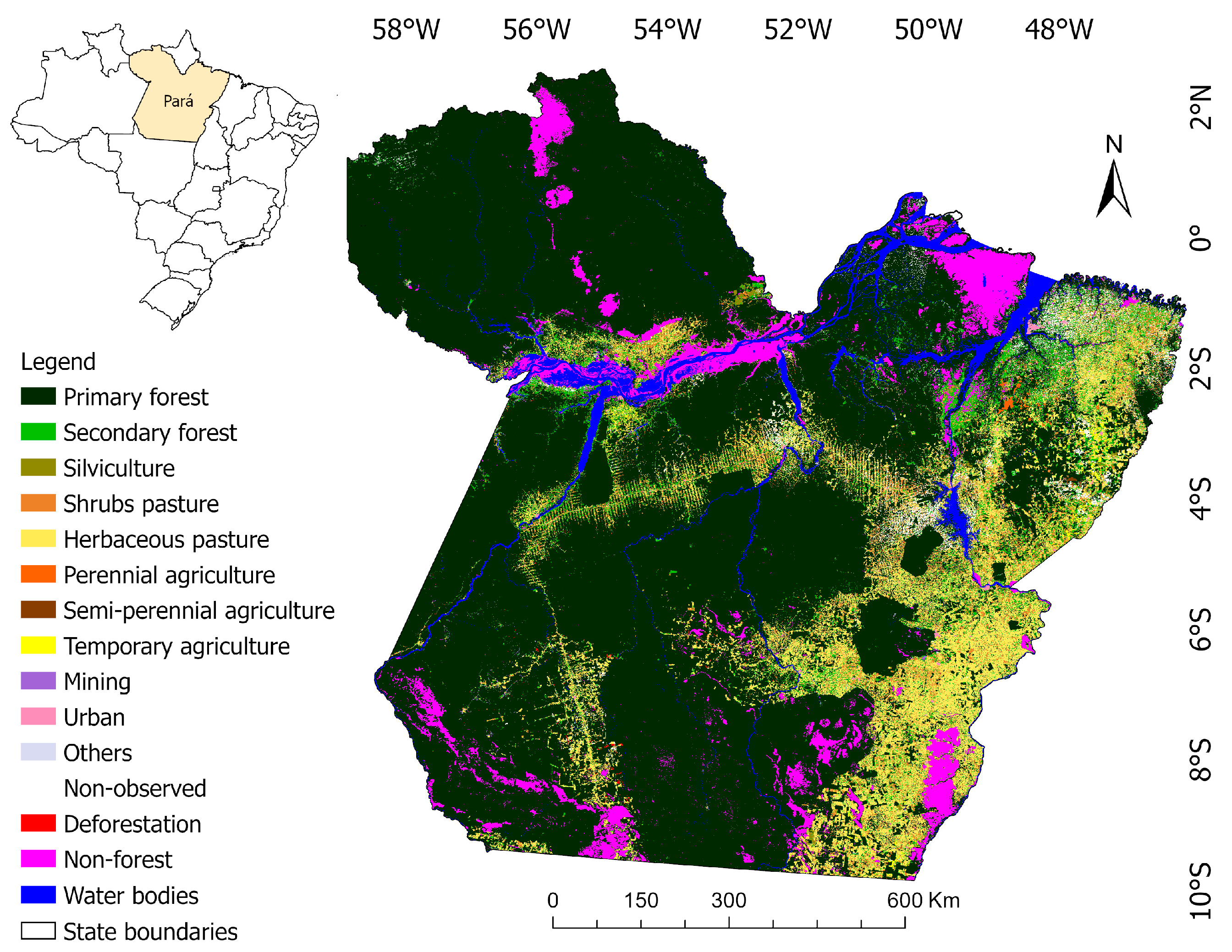
2.1. Study Area
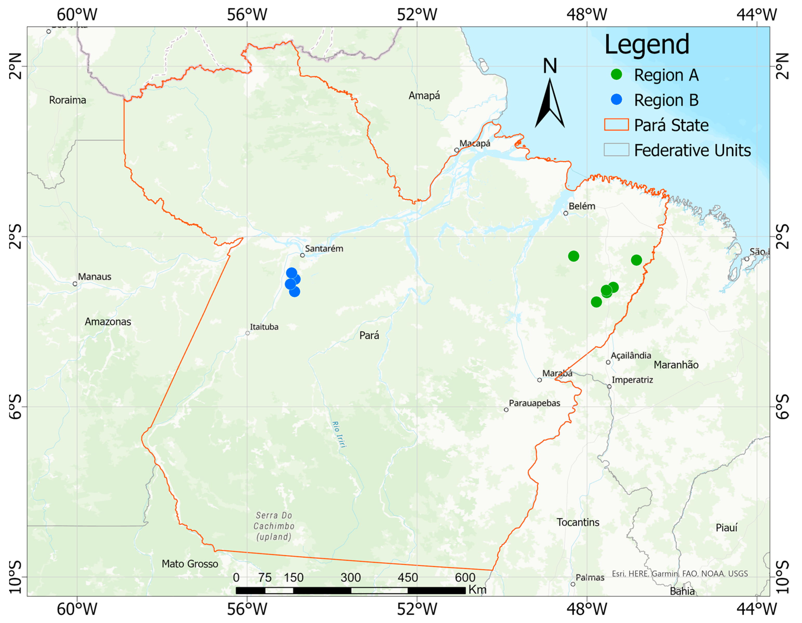
Pilot Areas
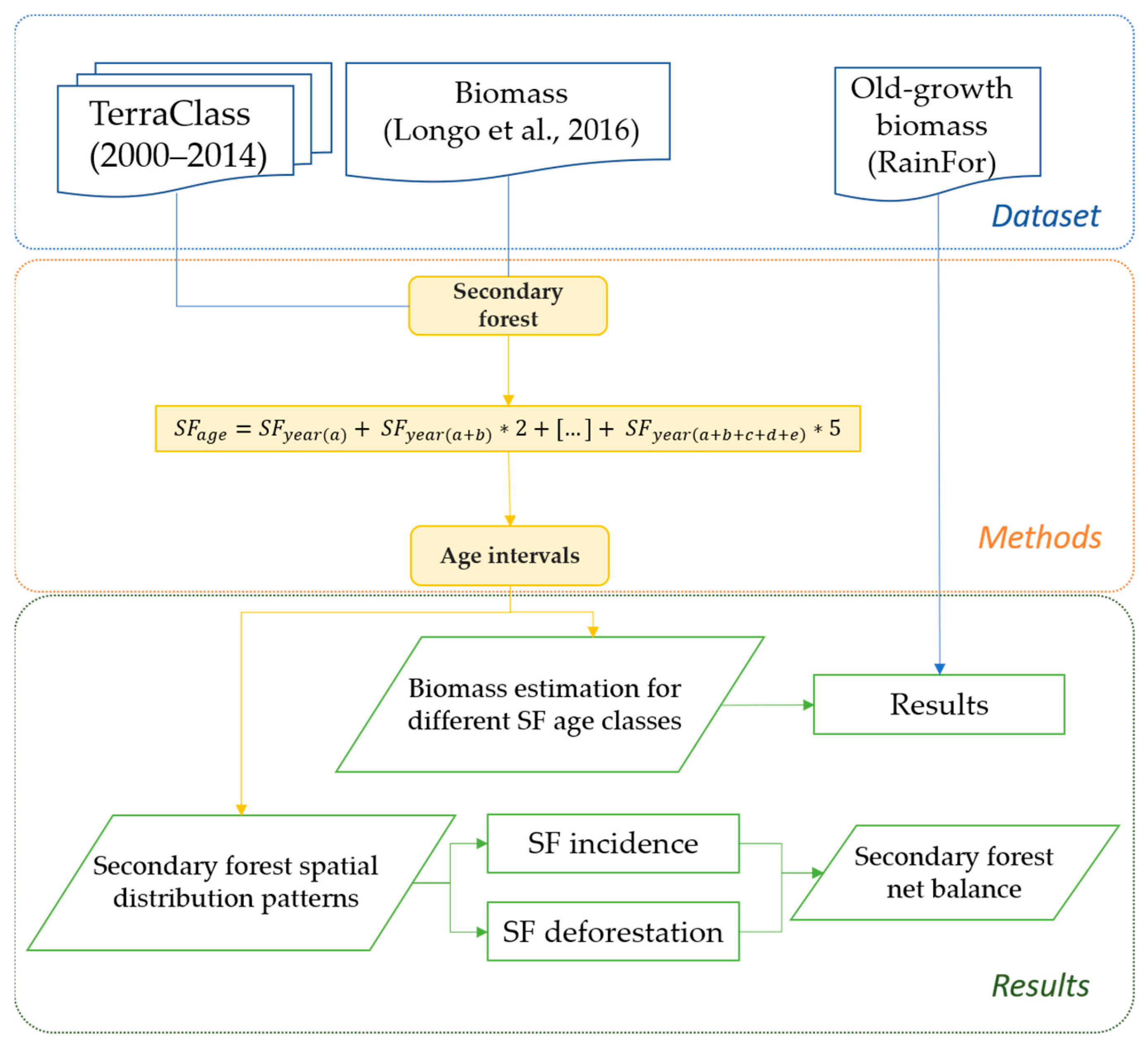
2.2. Methodological Approach
2.3. Land Use Change and Secondary Forest Age
2.4. Aboveground Biomass Estimation Data
2.5. Data Analysis
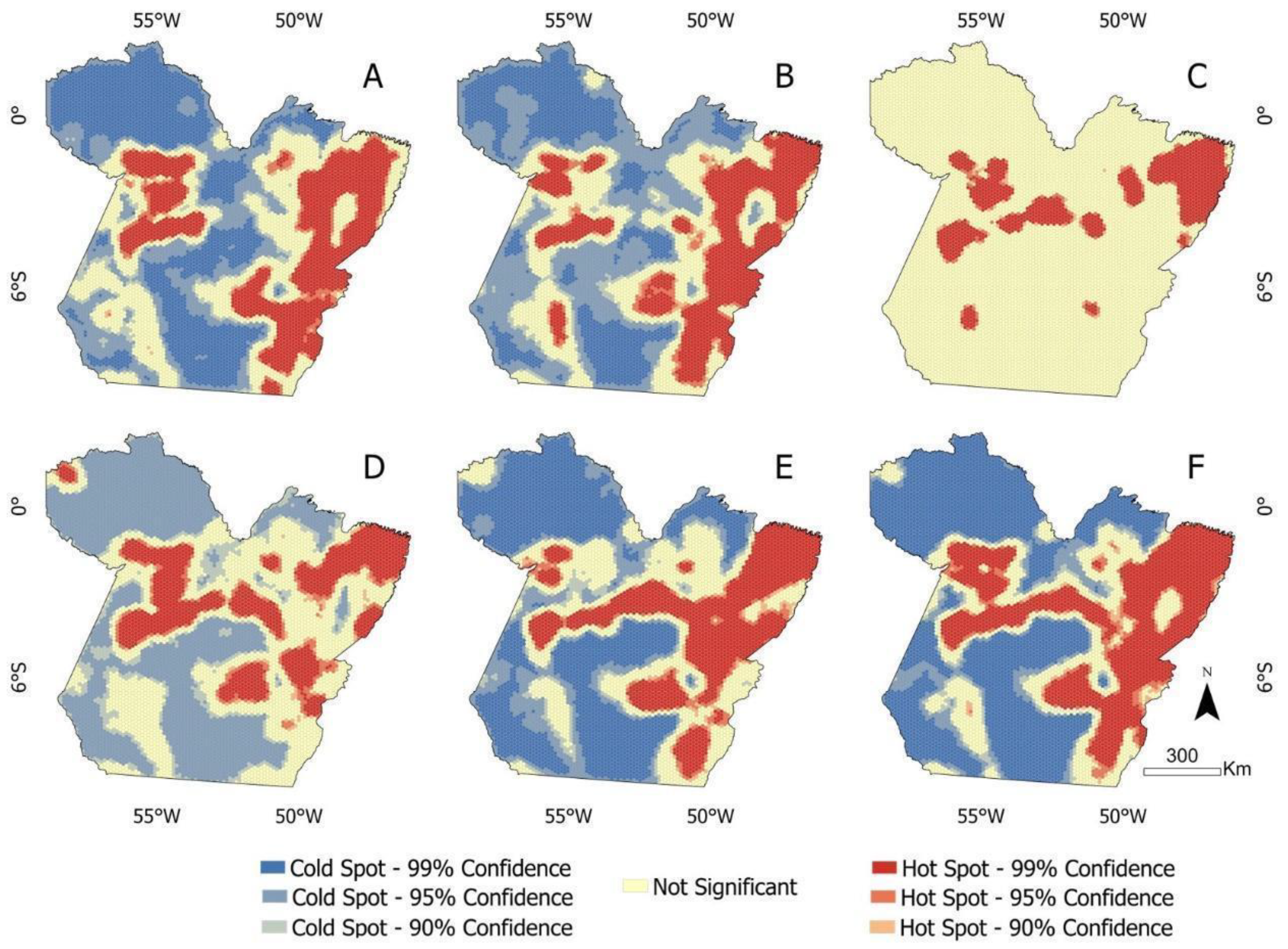
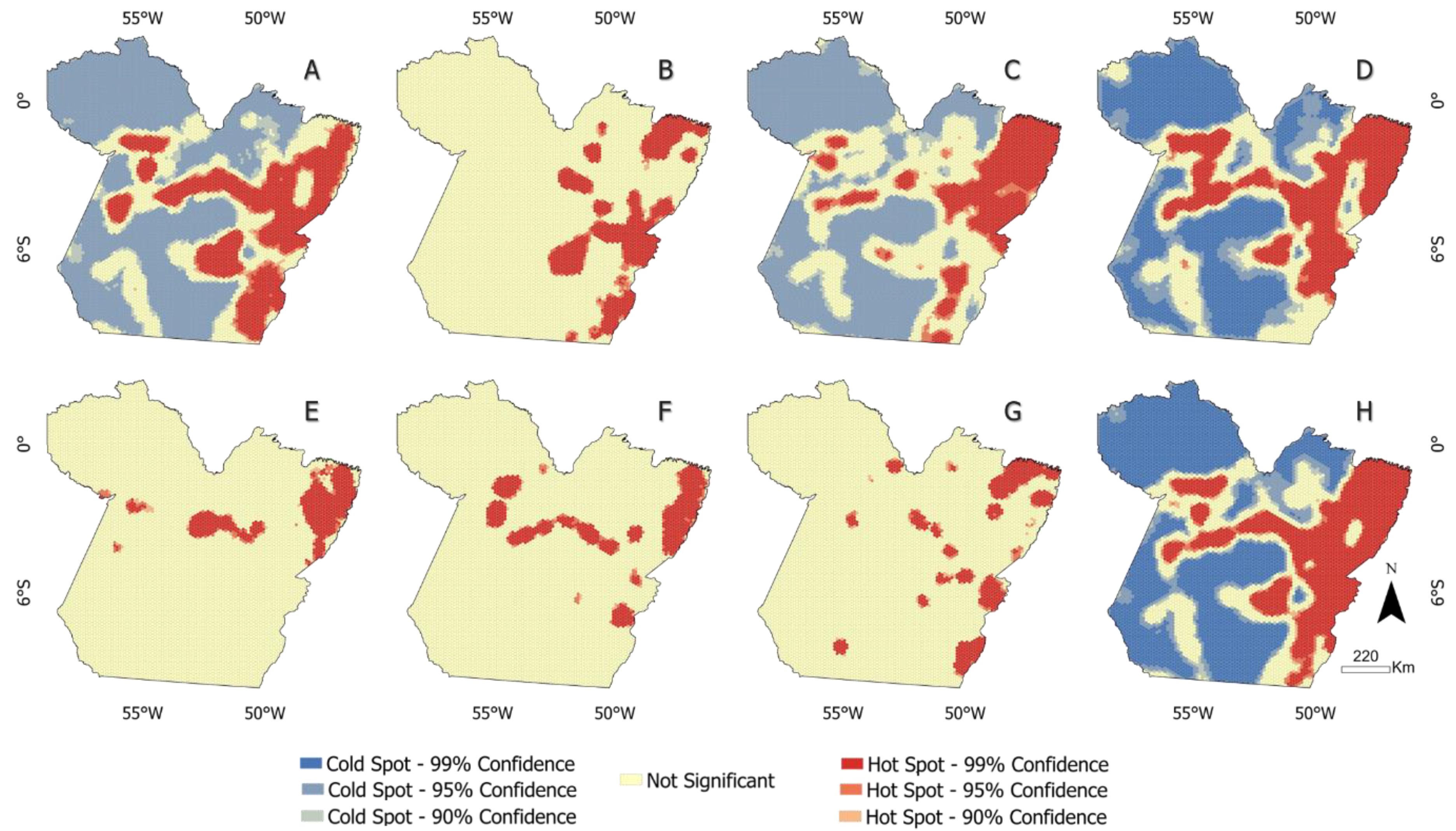
2.5.1. Hot Spot Analysis of Spatial Distribution of Secondary Forests
2.5.2. Hot Spot Analysis of Spatial Distribution of Deforestation in Secondary Forests
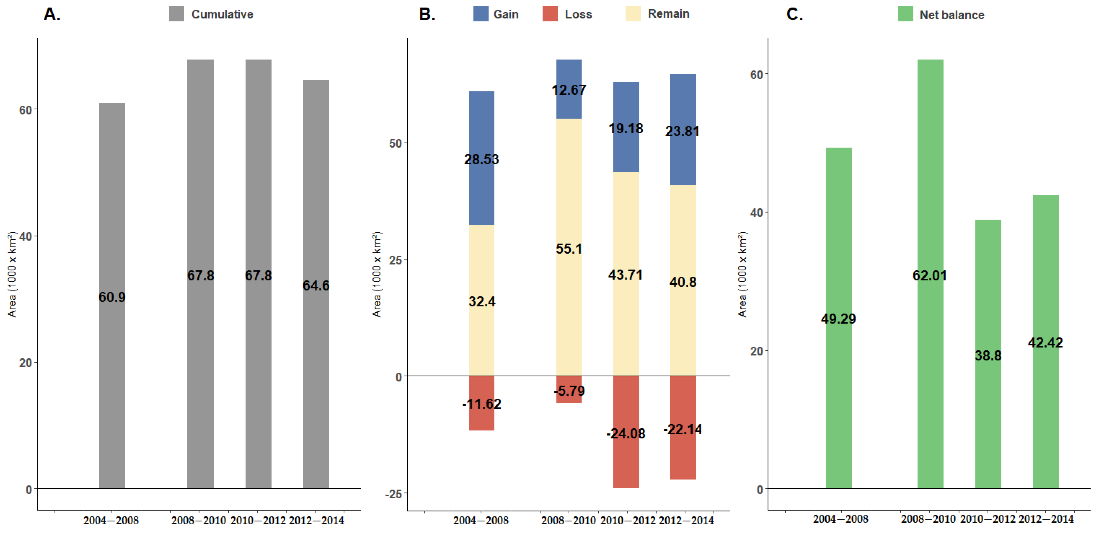
2.5.3. Secondary Forest Net Balance
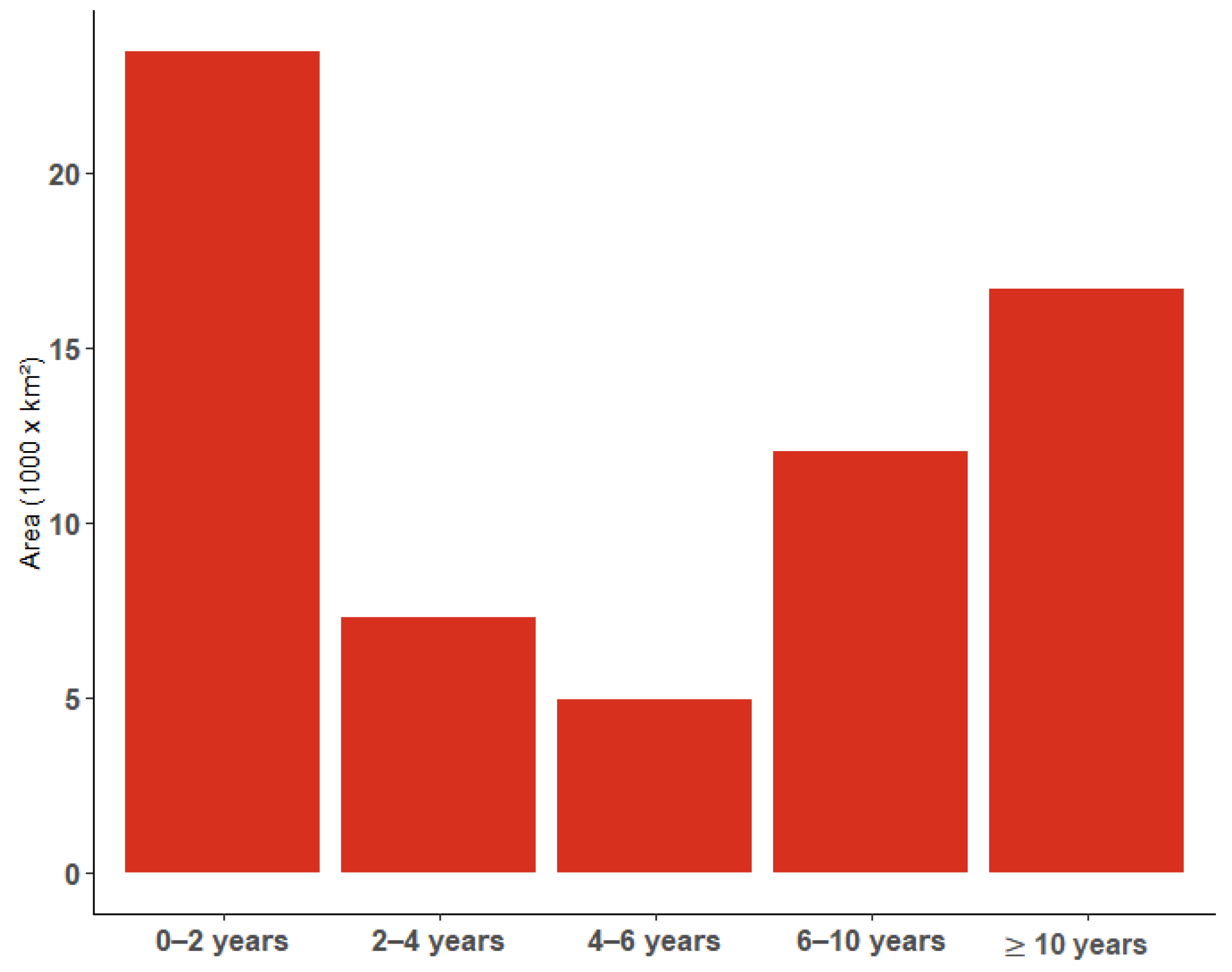
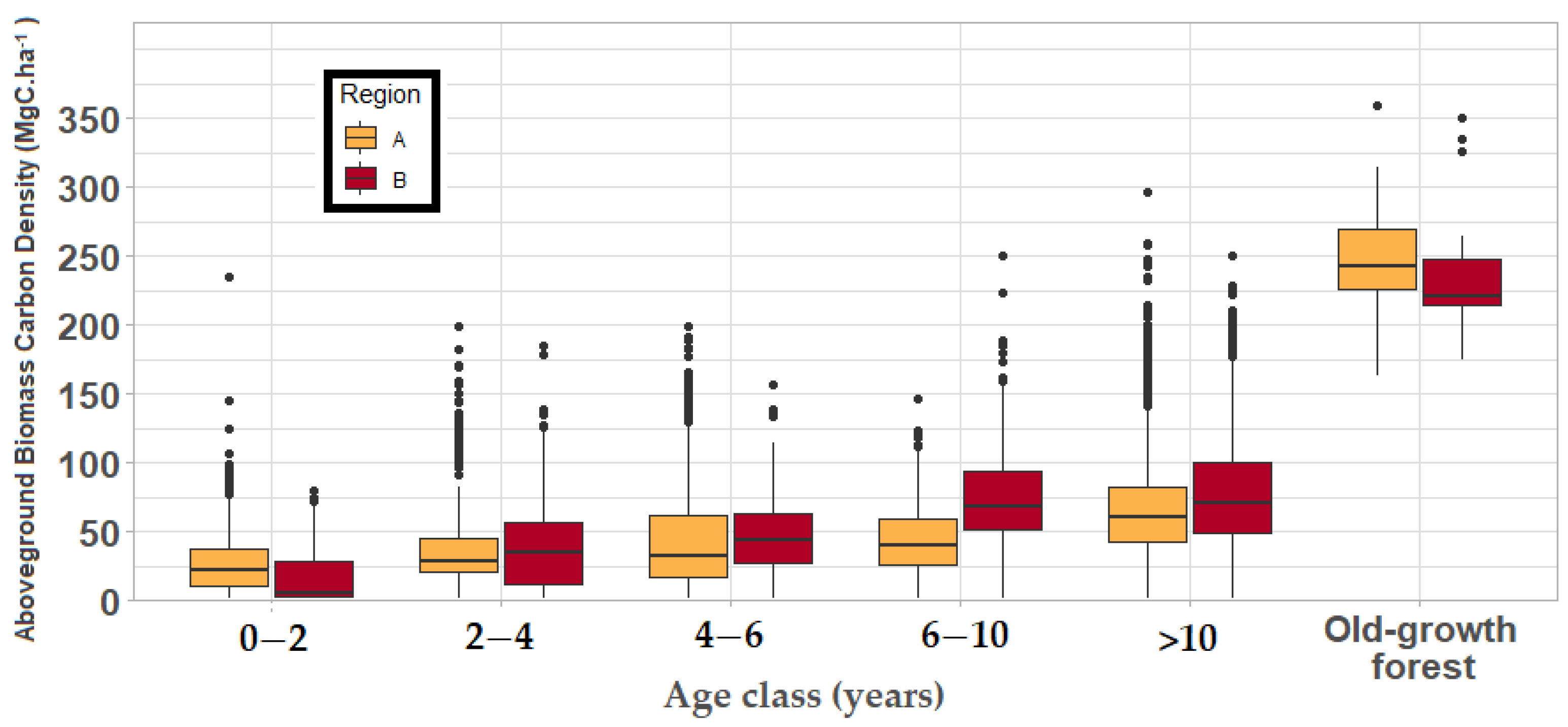
2.5.4. Aboveground Biomass Estimation for Different Secondary Forest Age Classes
3. Results
3.1. Secondary Forest Spatial Distribution Patterns
3.2. Secondary Forest Net Balance
3.3. Aboveground Biomass Estimation for Different Secondary Forest Age Classes
4. Discussion
5. Conclusions
Author Contributions
Funding
Data Availability Statement
Acknowledgments
Conflicts of Interest
References
- Vieira, I.C.G. Land Use Drives Change in Amazonian Tree Species. An. Acad. Bras. Cienc. 2019, 91. [Google Scholar] [CrossRef]
- Wang, Y.; Ziv, G.; Adami, M.; Almeida, C.A.D.; Antunes, J.F.G.; Coutinho, A.C.; Esquerdo, J.C.D.M.; Gomes, A.R.; Galbraith, D. Upturn in Secondary Forest Clearing Buffers Primary Forest Loss in the Brazilian Amazon. Nat. Sustain. 2020, 3, 290–295. [Google Scholar] [CrossRef]
- Perz, S.G.; Skole, D.L. Secondary Forest Expansion in the Brazilian Amazon and the Refinement of Forest Transition Theory. Soc. Nat. Resour. 2003, 16, 277–294. [Google Scholar] [CrossRef]
- Chazdon, R.L.; Broadbent, E.N.; Rozendaal, D.M.A.; Bongers, F.; Zambrano, A.M.A.; Aide, T.M.; Balvanera, P.; Becknell, J.M.; Boukili, V.; Brancalion, P.H.S.; et al. Carbon Sequestration Potential of Second-Growth Forest Regeneration in the Latin American Tropics. Sci. Adv. 2016, 2, e1501639. [Google Scholar] [CrossRef]
- Poorter, L.; Bongers, F.; Aide, T.M.; Almeyda Zambrano, A.M.; Balvanera, P.; Becknell, J.M.; Boukili, V.; Brancalion, P.H.S.; Broadbent, E.N.; Chazdon, R.L.; et al. Biomass Resilience of Neotropical Secondary Forests. Nature 2016, 530, 211–214. [Google Scholar] [CrossRef]
- Rozendaal, D.M.A.; Chazdon, R.L.; Arreola-Villa, F.; Balvanera, P.; Bentos, T.V.; Dupuy, J.M.; Hernández-Stefanoni, J.L.; Jakovac, C.C.; Lebrija-Trejos, E.E.; Lohbeck, M.; et al. Demographic Drivers of Aboveground Biomass Dynamics During Secondary Succession in Neotropical Dry and Wet Forests. Ecosystems 2017, 20, 340–353. [Google Scholar] [CrossRef]
- Heinrich, V.H.A.; Dalagnol, R.; Cassol, H.L.G.; Rosan, T.M.; de Almeida, C.T.; Silva Junior, C.H.L.; Campanharo, W.A.; House, J.I.; Sitch, S.; Hales, T.C.; et al. Large Carbon Sink Potential of Secondary Forests in the Brazilian Amazon to Mitigate Climate Change. Nat. Commun. 2021, 12, 1785. [Google Scholar] [CrossRef]
- Coutinho, A.C.; Almeida, C.; Venturieri, A.; Esquerdo, J.C.D.M.; Silva, M. Uso e Cobertura Da Terra Nas Áreas Desflorestadas Da Amazônia Legal: TerraClass 2008; Brasília. DF Embrapa; INPE: Belém, Brazil, 2013; ISBN 9788570351807. [Google Scholar]
- Almeida, C.A.d.; Coutinho, A.C.; Esquerdo, J.C.D.M.; Adami, M.; Venturieri, A.; Diniz, C.G.; Dessay, N.; Durieux, L.; Gomes, A.R. High Spatial Resolution Land Use and Land Cover Mapping of the Brazilian Legal Amazon in 2008 Using Landsat-5/TM and MODIS Data. Acta Amaz. 2016, 46, 291–302. [Google Scholar] [CrossRef]
- INPE PRODES-Monitoramento de Floresta Amazônica Brasileira Por Satelite. Available online: http://www.obt.inpe.br/OBT/assuntos/programas/amazonia/prodes (accessed on 26 April 2021).
- Lovejoy, T.E.; Nobre, C. Amazon Tipping Point. Sci. Adv. 2018, 4, eaat2340. [Google Scholar] [CrossRef] [PubMed]
- Marengo, J.; Nobre, C.A.; Betts, R.A.; Cox, P.M.; Sampaio, G.; Salazar, L. Global Warming and Climate Change in Amazonia: Climate-Vegetation Feedback and Impacts on Water Resources. In Amazonia and Global Change; American Geophysical Union: Washington, DC, USA, 2009; pp. 273–292. ISBN 9781118670347. [Google Scholar]
- Fearnside, P.M. Desmatamento Na Amazônia: Dinâmica, Impactos e Controle. Acta Amaz. 2006, 36, 395–400. [Google Scholar] [CrossRef]
- MapBiomas Projeto MapBiomas−Coleção 6 Da Série Anual de Mapas de Cobertura e Uso de Solo Do Brasil. Available online: https://plataforma.mapbiomas.org/ (accessed on 10 October 2021).
- Silva Junior, C.H.L.; Heinrich, V.H.A.; Freire, A.T.G.; Broggio, I.S.; Rosan, T.M.; Doblas, J.; Anderson, L.O.; Rousseau, G.X.; Shimabukuro, Y.E.; Silva, C.A.; et al. Benchmark Maps of 33 Years of Secondary Forest Age for Brazil. Sci. Data 2020, 7, 269. [Google Scholar] [CrossRef] [PubMed]
- Saldarriaga, J.G.; West, D.C.; Tharp, M.L.; Uhl, C. Long-Term Chronosequence of Forest Succession in the Upper Rio Negro of Colombia and Venezuela. J. Ecol. 1988, 76, 938. [Google Scholar] [CrossRef]
- Fearnside, P.M. Amazonian Deforestation and Global Warming: Carbon Stocks in Vegetation Replacing Brazil’s Amazon Forest. For. Ecol. Manag. 1996, 80, 21–34. [Google Scholar] [CrossRef]
- Uhl, C.; Buschbacher, R.; Serrao, E.A.S. Abandoned Pastures in Eastern Amazonia. I. Patterns of Plant Succession. J. Ecol. 1988, 76, 663. [Google Scholar] [CrossRef]
- Nelson, R.F.; Kimes, D.S.; Salas, W.A.; Routhier, M. Secondary Forest Age and Tropical Forest Biomass Estimation Using Thematic Mapper Imagery. Bioscience 2000, 50, 419–431. [Google Scholar] [CrossRef]
- Carrasco, R.A.; Pinheiro, M.M.F.; Junior, J.M.; Cicerelli, R.E.; Silva, P.A.; Osco, L.P.; Ramos, A.P.M. Land Use/Land Cover Change Dynamics and Their Effects on Land Surface Temperature in the Western Region of the State of São Paulo, Brazil. Reg. Environ. Chang. 2020, 20, 96. [Google Scholar] [CrossRef]
- Nelson, B.W.; Mesquita, R.; Pereira, J.L.; Garcia Aquino de Souza, S.; Teixeira Batista, G.; Bovino Couto, L. Allometric Regressions for Improved Estimate of Secondary Forest Biomass in the Central Amazon. For. Ecol. Manag. 1999, 117, 149–167. [Google Scholar] [CrossRef]
- Saatchi, S.S.; Houghton, R.A.; Dos Santos Alvalá, R.C.; Soares, J.V.; Yu, Y. Distribution of Aboveground Live Biomass in the Amazon Basin. Glob. Chang. Biol. 2007, 13, 816–837. [Google Scholar] [CrossRef]
- Longo, M.; Keller, M.; Dos-Santos, M.N.; Leitold, V.; Pinagé, E.R.; Baccini, A.; Saatchi, S.; Nogueira, E.M.; Batistella, M.; Morton, D.C. Aboveground Biomass Variability across Intact and Degraded Forests in the Brazilian Amazon. Glob. Biogeochem. Cycles 2016, 30, 1639–1660. [Google Scholar] [CrossRef]
- Smith, C.C.; Espírito-Santo, F.D.B.; Healey, J.R.; Young, P.J.; Lennox, G.D.; Ferreira, J.; Barlow, J. Secondary Forests Offset Less than 10% of Deforestation-mediated Carbon Emissions in the Brazilian Amazon. Glob. Chang. Biol. 2020, 26, 7006–7020. [Google Scholar] [CrossRef] [PubMed]
- Chazdon, R.L.; Letcher, S.G.; van Breugel, M.; Martínez-Ramos, M.; Bongers, F.; Finegan, B. Rates of Change in Tree Communities of Secondary Neotropical Forests Following Major Disturbances. Philos. Trans. R. Soc. B Biol. Sci. 2007, 362, 273–289. [Google Scholar] [CrossRef] [PubMed]
- Chazdon, R.L.; Peres, C.A.; Dent, D.; Sheil, D.; Lugo, A.E.; Lamb, D.; Stork, N.E.; Miller, S.E. The Potential for Species Conservation in Tropical Secondary Forests. Conserv. Biol. 2009, 23, 1406–1417. [Google Scholar] [CrossRef] [PubMed]
- Cassol, H.L.G.; De Oliveira E Cruz De Aragão, L.E.; Moraes, E.C.; Carreiras, J.M.d.B.; Shimabukuro, Y.E. Quad-Pol Advanced Land Observing Satellite/Phased Array L-Band Synthetic Aperture Radar-2 (ALOS/PALSAR-2) Data for Modelling Secondary Forest above-Ground Biomass in the Central Brazilian Amazon. Int. J. Remote Sens. 2021, 42, 4985–5009. [Google Scholar] [CrossRef]
- Baccini, A.; Goetz, S.J.; Walker, W.S.; Laporte, N.T.; Sun, M.; Sulla-Menashe, D.; Hackler, J.; Beck, P.S.A.; Dubayah, R.; Friedl, M.A.; et al. Estimated Carbon Dioxide Emissions from Tropical Deforestation Improved by Carbon-Density Maps. Nat. Clim. Chang. 2012, 2, 182–185. [Google Scholar] [CrossRef]
- Requena Suarez, D.; Rozendaal, D.M.A.; De Sy, V.; Phillips, O.L.; Alvarez-Dávila, E.; Anderson-Teixeira, K.; Araujo-Murakami, A.; Arroyo, L.; Baker, T.R.; Bongers, F.; et al. Estimating Aboveground Net Biomass Change for Tropical and Subtropical Forests: Refinement of IPCC Default Rates Using Forest Plot Data. Glob. Chang. Biol. 2019, 25, 3609–3624. [Google Scholar] [CrossRef]
- IBGE Área Territorial Brasileira 2020; IBGE: Rio de Janeiro, Brazil, 2021.
- Guimarães, J.; Veríssimo, A.; Amaral, P.; Demachki, A. Municipios Verdes: Caminhos Para a Sustentabilidade; Barreto, G., Veríssimo, T.C., Eds.; Imazon: Belém, Brazil, 2011; ISBN 9788586212376. [Google Scholar]
- Tomlin, C.D. Geographic Information Systems and Cartographic Modeling; Prentice Hall: Hoboken, NJ, USA, 1990; ISBN 978-0133509274. [Google Scholar]
- Lopez-Gonzalez, G.; Lewis, S.L.; Burkitt, M.; Phillips, O.L. ForestPlots.Net: A Web Application and Research Tool to Manage and Analyse Tropical Forest Plot Data. J. Veg. Sci. 2011, 22, 610–613. [Google Scholar] [CrossRef]
- Mitchell, A. The ESRI Guide to GIS Analysis, Volume 2: Spatial Measurements and Statistics; ESRI Press: Redlands, CA, USA, 2005; ISBN 9781589481169. [Google Scholar]
- Elias, F.; Ferreira, J.; Lennox, G.D.; Berenguer, E.; Ferreira, S.; Schwartz, G.; Melo, L.d.O.; Reis Júnior, D.N.; Nascimento, R.O.; Ferreira, F.N.; et al. Assessing the Growth and Climate Sensitivity of Secondary Forests in Highly Deforested Amazonian Landscapes. Ecology 2020, 101, e02954. [Google Scholar] [CrossRef] [PubMed]
- Aragão, L.E.O.C.; Poulter, B.; Barlow, J.B.; Anderson, L.O.; Malhi, Y.; Saatchi, S.; Phillips, O.L.; Gloor, E. Environmental Change and the Carbon Balance of Amazonian Forests. Biol. Rev. 2014, 89, 913–931. [Google Scholar] [CrossRef]
- Whately, M.; Campanili, M. Programa Municípios Verdes: Lições Aprendidas e Desafios Para 2013/2014; Campanili, M., Ed.; Governo do Estado: Belém, Brazil, 2013; ISBN 9788586212512. [Google Scholar]
- Pinto, A.; Amaral, P.; Souza, A., Jr.; Veríssimo, A.; Salomão, R.; Gomes, G.; Balieiro, C. Diagnostico Socioeconômico e Florestal Do Município de Paragominas; Imazon: Belém, Brazil, 2009. [Google Scholar]
- Wandelli, E.V.; Fearnside, P.M. Secondary Vegetation in Central Amazonia: Land-Use History Effects on Aboveground Biomass. For. Ecol. Manag. 2015, 347, 140–148. [Google Scholar] [CrossRef]
- Holl, K.D. Factors Limiting Tropical Rain Forest Regeneration in Abandoned Pasture: Seed Rain, Seed Germination, Microclimate, and Soil1. Biotropica 1999, 31, 229–242. [Google Scholar] [CrossRef]
- Wang, Y.; Ziv, G.; Adami, M.; Mitchard, E.; Batterman, S.A.; Buermann, W.; Schwantes Marimon, B.; Marimon Junior, B.H.; Matias Reis, S.; Rodrigues, D.; et al. Mapping Tropical Disturbed Forests Using Multi-Decadal 30 m Optical Satellite Imagery. Remote Sens. Environ. 2019, 221, 474–488. [Google Scholar] [CrossRef]
- Baker, T.R.; Phillips, O.L.; Malhi, Y.; Almeida, S.; Arroyo, L.; Di Fiore, A.; Erwin, T.; Killeen, T.J.; Laurance, S.G.; Laurance, W.F.; et al. Variation in Wood Density Determines Spatial Patterns InAmazonian Forest Biomass. Glob. Chang. Biol. 2004, 10, 545–562. [Google Scholar] [CrossRef]
- Rozendaal, D.M.A.; Requena Suarez, D.; De Sy, V.; Avitabile, V.; Carter, S.; Adou Yao, C.Y.; Alvarez-Davila, E.; Anderson-Teixeira, K.; Araujo-Murakami, A.; Arroyo, L.; et al. Aboveground Forest Biomass Varies across Continents, Ecological Zones and Successional Stages: Refined IPCC Default Values for Tropical and Subtropical Forests. Environ. Res. Lett. 2022, 17, 014047. [Google Scholar] [CrossRef]
- Becknell, J.M.; Kissing Kucek, L.; Powers, J.S. Aboveground Biomass in Mature and Secondary Seasonally Dry Tropical Forests: A Literature Review and Global Synthesis. For. Ecol. Manag. 2012, 276, 88–95. [Google Scholar] [CrossRef]
- Eggleston, H.S.; Buendia, L.; Miwa, K.; Ngara, T.; Tanabe, K. 2006 IPCC Guidelines for Natinal Greenhouse Gas Inventories; IGES: Hayama, Japan, 2008. [Google Scholar]
- 2019 Refinement to the 2006 IPCC Guidelines for National Greenhouse Gas Inventories: Agriculture, Forestry and Other Land Use; IGES: Hayama, Japan, 2019.
- Carvalho, R.; Adami, M.; Amaral, S.; Bezerra, F.G.; de Aguiar, A.P.D. Changes in Secondary Vegetation Dynamics in a Context of Decreasing Deforestation Rates in Pará, Brazilian Amazon. Appl. Geogr. 2019, 106, 40–49. [Google Scholar] [CrossRef]
- Leitold, V.; Keller, M.; Morton, D.C.; Cook, B.D.; Shimabukuro, Y.E. Airborne Lidar-Based Estimates of Tropical Forest Structure in Complex Terrain: Opportunities and Trade-Offs for REDD+. Carbon Balance Manag. 2015, 10, 3. [Google Scholar] [CrossRef]
- GEDI Ecosystem Lidar Global Ecosystem Dynamics Investigation (GEDI). Available online: https://gedi.umd.edu/ (accessed on 18 April 2023).
- Hélière, F.; Fois, F.; Arcioni, M.; Bensi, P.; Fehringer, M.; Scipal, K. Biomass P-Band SAR Interferometric Mission Selected as 7th Earth Explorer Mission. In Proceedings of the Proceedings of the European Conference on Synthetic Aperture Radar, EUSAR, Berlin, Germany, 3–5 June 2014; Volume Proceeding, pp. 1152–1155. [Google Scholar]


| Age Interval (Years) | Class | 2004 | 2008 | 2010 | 2012 | 2014 |
|---|---|---|---|---|---|---|
| 0 to 2 | 1 | Non-Secondary Forest | Non-Secondary Forest | Non-Secondary Forest | Non-Secondary Forest | Secondary Forest |
| 2 to 4 | 2 | Non-Secondary Forest | Non-Secondary Forest | Non-Secondary Forest | Secondary Forest | Secondary Forest |
| 4 to 6 | 3 | Non-Secondary Forest | Non-Secondary Forest | Secondary Forest | Secondary Forest | Secondary Forest |
| 6 to 10 | 4 | Non-Secondary Forest | Secondary Forest | Secondary Forest | Secondary Forest | Secondary Forest |
| >10 | 5 | Secondary Forest | Secondary Forest | Secondary Forest | Secondary Forest | Secondary Forest |
| Age Interval (Years) | Region A | Region B | ||||||
|---|---|---|---|---|---|---|---|---|
| N | N | |||||||
| 0 to 2 | 27.11 | 20.98 | 439 | 2326 | 17.18 | 19.67 | 387 | 155 |
| 2 to 4 | 43.48 | 38.67 | 1492 | 545 | 38.17 | 31.46 | 990 | 478 |
| 4 to 6 | 45.96 | 40.67 | 1654 | 1333 | 46.18 | 32.57 | 1061 | 141 |
| 6 to 10 | 43.97 | 24.03 | 576 | 1835 | 75.86 | 43.72 | 1911 | 284 |
| >10 | 66.00 | 37.00 | 1369 | 4508 | 77.01 | 39.22 | 1538 | 2828 |
| Old-growth forest | 287.07 | 95.50 | 9120 | 13 | 235.50 | 41.78 | 1745 | 29 |
| Source of Variation | Df | Sum Sq | Fvalue | Pr (>F) |
|---|---|---|---|---|
| (Intercept) | 1 | 1,709,123 | 1454.573 | <2.2 × 10⁻¹⁶ *** |
| Age class | 5 | 32,15,260 | 547.279 | <2.2 × 10⁻¹⁶ *** |
| Region | 1 | 14,319 | 12.187 | 0.0004828 *** |
| Age class + Region | 5 | 282,406 | 48.069 | <2.2 × 10⁻¹⁶ *** |
| Residuals | 14,469 | 16,995,190 |
| Interaction | diff | lwr | upr | p adj |
|---|---|---|---|---|
| B−A | 8.311 | 7.054 | 9.569 | 0.000 |
| A−1−A−2 | 16.374 | 11.042 | 21.706 | 0.000 |
| A−1−A−3 | 18.855 | 15.007 | 22.703 | 0.000 |
| A−1−A−4 | 16.862 | 13.364 | 20.360 | 0.000 |
| A−1−A−5 | 38.895 | 36.034 | 41.755 | 0.000 |
| A−1−A−7 | 259.966 | 228.805 | 291.127 | 0.000 |
| B−1−A−1 | −9.927 | −19.221 | −0.632 | 0.024 |
| B−1−A−2 | 11.067 | 5.440 | 16.693 | 0.000 |
| B−1−A−3 | 19.071 | 9.354 | 28.789 | 0.000 |
| B−1−A−4 | 48.757 | 41.715 | 55.800 | 0.000 |
| B−1−A−5 | 49.899 | 46.763 | 53.035 | 0.000 |
| B−1−A−7 | 208.398 | 187.463 | 229.333 | 0.000 |
| A−2−A−3 | 2.481 | −3.215 | 8.177 | 0.959 |
| A−2−A−4 | 0.488 | −4.977 | 5.954 | 1.000 |
| A−2−A−5 | 22.521 | 17.440 | 27.602 | 0.000 |
| A−2−A−7 | 243.592 | 212.149 | 275.035 | 0.000 |
| B−2−A−1 | −26.300 | −36.499 | −16.101 | 0.000 |
| B−2−A−2 | −5.307 | −12.328 | 1.714 | 0.359 |
| B−2−A−3 | 2.698 | −7.888 | 13.284 | 1.000 |
| B−2−A−4 | 32.384 | 24.184 | 40.583 | 0.000 |
| B−2−A−5 | 33.525 | 28.284 | 38.767 | 0.000 |
| B−2−A−7 | 192.024 | 170.673 | 213.376 | 0.000 |
| A−3−A−4 | −1.993 | −6.024 | 2.039 | 0.904 |
| A−3−A−5 | 20.040 | 16.548 | 23.532 | 0.000 |
| A−3−A−7 | 241.111 | 209.886 | 272.337 | 0.000 |
| B−3−A−1 | −28.781 | −38.289 | −19.274 | 0.000 |
| B−3−A−2 | −7.788 | −13.761 | −1.816 | 0.001 |
| B−3−A−3 | 0.217 | −9.705 | 10.138 | 1.000 |
| B−3−A−4 | 29.903 | 22.581 | 37.225 | 0.000 |
| B−3−A−5 | 31.045 | 27.323 | 34.766 | 0.000 |
| B−3−A−7 | 189.543 | 168.513 | 210.574 | 0.000 |
| A−4−A−5 | 22.033 | 18.930 | 25.135 | 0.000 |
| A−4−A−7 | 243.104 | 211.920 | 274.288 | 0.000 |
| B−4−A−1 | −26.789 | −36.160 | −17.417 | 0.000 |
| B−4−A−2 | −5.795 | −11.549 | −0.042 | 0.046 |
| B−4−A−3 | 2.209 | −7.582 | 12.001 | 1.000 |
| B−4−A−4 | 31.895 | 24.751 | 39.040 | 0.000 |
| B−4−A−5 | 33.037 | 29.679 | 36.396 | 0.000 |
| B−4−A−7 | 191.536 | 170.567 | 212.505 | 0.000 |
| A−5−A−7 | 221.071 | 189.952 | 252.190 | 0.000 |
| B−5−A−1 | −48.821 | −57.974 | −39.669 | 0.000 |
| B−5−A−2 | −27.828 | −33.217 | −22.439 | 0.000 |
| B−5−A−3 | −19.823 | −29.405 | −10.241 | 0.000 |
| B−5−A−4 | 9.863 | 3.008 | 16.717 | 0.000 |
| B−5−A−5 | 11.005 | 8.317 | 13.692 | 0.000 |
| B−5−A−7 | 169.503 | 148.631 | 190.375 | 0.000 |
| B−7−A−1 | −269.892 | −302.244 | −237.541 | 0.000 |
| B−7−A−2 | −248.899 | −280.393 | −217.405 | 0.000 |
| B−7−A−3 | −240.894 | −273.370 | −208.419 | 0.000 |
| B−7−A−4 | −211.209 | −242.986 | −179.431 | 0.000 |
| B−7−A−5 | −210.067 | −241.212 | −178.921 | 0.000 |
| B−7−A−7 | −51.568 | −88.964 | −14.172 | 0.000 |
| B−1−B−2 | 20.993 | 10.637 | 31.349 | 0.000 |
| B−1−B−3 | 28.998 | 15.959 | 42.037 | 0.000 |
| B−1−B−4 | 58.684 | 47.495 | 69.873 | 0.000 |
| B−1−B−5 | 59.826 | 50.583 | 69.068 | 0.000 |
| B−1−B−7 | 218.325 | 195.656 | 240.993 | 0.000 |
| B−2−B−3 | 8.005 | −2.733 | 18.742 | 0.381 |
| B−2−B−4 | 37.691 | 29.297 | 46.085 | 0.000 |
| B−2−B−5 | 38.833 | 33.292 | 44.373 | 0.000 |
| B−2−B−7 | 197.331 | 175.904 | 218.759 | 0.000 |
| B−3−B−4 | 29.686 | 18.143 | 41.228 | 0.000 |
| B−3−B−5 | 30.828 | 21.160 | 40.496 | 0.000 |
| B−3−B−7 | 189.327 | 166.482 | 212.172 | 0.000 |
| B−4−B−5 | 1.142 | −5.832 | 8.116 | 1.000 |
| B−4−B−7 | 159.641 | 137.799 | 181.482 | 0.000 |
| B−5−B−7 | 158.499 | 137.587 | 179.410 | 0.000 |
Disclaimer/Publisher’s Note: The statements, opinions and data contained in all publications are solely those of the individual author(s) and contributor(s) and not of MDPI and/or the editor(s). MDPI and/or the editor(s) disclaim responsibility for any injury to people or property resulting from any ideas, methods, instructions or products referred to in the content. |
© 2023 by the authors. Licensee MDPI, Basel, Switzerland. This article is an open access article distributed under the terms and conditions of the Creative Commons Attribution (CC BY) license (https://creativecommons.org/licenses/by/4.0/).
Share and Cite
da Silva, G.M.; Adami, M.; Galbraith, D.; Nascimento, R.G.M.; Wang, Y.; Shimabukuro, Y.E.; Emmert, F. Spatial Distribution of Secondary Forests by Age Group and Biomass Accumulation in the Brazilian Amazon. Forests 2023, 14, 924. https://0-doi-org.brum.beds.ac.uk/10.3390/f14050924
da Silva GM, Adami M, Galbraith D, Nascimento RGM, Wang Y, Shimabukuro YE, Emmert F. Spatial Distribution of Secondary Forests by Age Group and Biomass Accumulation in the Brazilian Amazon. Forests. 2023; 14(5):924. https://0-doi-org.brum.beds.ac.uk/10.3390/f14050924
Chicago/Turabian Styleda Silva, Gabriel M., Marcos Adami, David Galbraith, Rodrigo G. M. Nascimento, Yunxia Wang, Yosio E. Shimabukuro, and Fabiano Emmert. 2023. "Spatial Distribution of Secondary Forests by Age Group and Biomass Accumulation in the Brazilian Amazon" Forests 14, no. 5: 924. https://0-doi-org.brum.beds.ac.uk/10.3390/f14050924