
UAV Multispectral Imagery Predicts Dead Fuel Moisture Content


College of Computer and Control Engineering, Northeast Forestry University, Harbin 150040, China
*
Author to whom correspondence should be addressed.
Forests 2023, 14(9), 1724; https://0-doi-org.brum.beds.ac.uk/10.3390/f14091724
Submission received: 19 June 2023
/
Revised: 29 July 2023
/
Accepted: 13 August 2023
/
Published: 26 August 2023
(This article belongs to the Special Issue Deep Learning Techniques for Forest Parameter Retrieval and Accurate Tree Modeling from Remote Sensing Data)
Abstract
:Forest floor dead fuel moisture content (DFMC) is an important factor in the occurrence of forest fires, and predicting DFMC is important for accurate fire risk forecasting. Large areas of forest surface DFMC are difficult to predict via manual methods. In this paper, we propose an unmanned aerial vehicle (UAV)-based forest surface DFMC prediction method, in which a UAV is equipped with a multispectral camera to collect multispectral images of dead combustible material on the forest surface over a large area, combined with a deep-learning algorithm to achieve the large-scale prediction of DFMC on the forest surface. From 9 March to 23 March 2023, 5945 multispectral images and 480 sets of dead combustible samples were collected from an urban forestry demonstration site in Harbin, China, using an M300 RTK UAV with an MS600Pro multispectral camera. The multispectral images were segmented by a K-means clustering algorithm to obtain multispectral images containing only dead combustibles on the ground surface. The segmented multispectral images were then trained with the actual moisture content measured by the weighing method through the ConvNeXt deep-learning model, with 3985 images as the training set, 504 images as the validation set, and 498 images as the test set. The results showed that the MAE and RMSE of the test set are 1.54% and 5.45%, respectively, and the accuracy is 92.26% with high precision, achieving the accurate prediction of DFMC over a large range. The proposed new method for predicting DFMC via UAV multispectral cameras is expected to solve the real-time large-range accurate prediction of the moisture content of dead combustible material on the forest surface during the spring fire-prevention period in northeast China, thus providing technical support for improving the accuracy of forest fire risk-level forecasting and forest fire spread trend prediction.
1. Introduction
Forest fires are a common natural disaster that can cause significant damage to both humans and the natural environment. Globally, raging forest fires affect biodiversity, wildlife habitat, and ecosystem attributes. About 84% of the world’s ecoregions are threatened by forest fires, severely affecting biodiversity. Forests, which play an important role in carbon sinks, may become a source of carbon to the atmosphere even after forest fires due to the death of trees in fire-affected areas [1]. According to the Fifth Assessment Report of the Intergovernmental Panel on Climate Change (IPCC), annual carbon emissions from forest fires range from 2.5 to 4 billion tons of carbon dioxide [2]. Forest burning degrades air quality due to the emission of large amounts of particulate matter and trace gases [3]. The average concentrations of particulate matter (PM2.5 and PM10) and nitrogen dioxide increase in areas affected by forest fires [4]. Land degradation due to forest fires is also a common problem. As a result of forest fires, large amounts of ash, carbon, and toxic substances are produced and contaminate the air, water, and soil, and the contaminated air, water, and soil affect soil nutrients and microorganisms, altering the productivity of the soil. Between 2000 and 2020, the average number of fires per year in China was 6283 (with a range of 1153 to 14,144 fires), and the average area burned was 183,126 hectares (ranging from 18,161 to 1,123,751 ha) [5].
Forest fuels are materials that can be burned in forests with a source of fire and oxygen, while dead forest surface fuels are fuels with a time lag of less than 10 h [6]. These include mainly fallen fine dead leaves, of which fine dead fuels with a time lag of 1 h play an important role in fire risk-forecasting systems as they dry out or become wet quickly [7]. The key to forest fire weather forecasting and fire behavior forecasting is the accurate prediction of surface dead fuel moisture content (DFMC) [8]. Forest fuels are one of the three main elements in the occurrence of forest fires and the material basis for forest burning. When the moisture content of forest surface fuels is low, i.e., dry, flammable materials such as dead leaves and branches burn easily and fires spread easily, thus increasing the risk of forest fires [9]. On the other hand, when the moisture content of forest surface fuels is high, the moisture in the burning material can stop the spread of fire, effectively reducing the risk of fire [10]. Therefore, predicting the moisture content of forest surface fuels can help predict the risk of forest fires and take timely measures to reduce the damage caused by fire to humans and the natural environment.
Research methods for forest fuel moisture content have so far been lacking in terms of techniques and methods for directly measuring the moisture content of forest ground cover fuels, and there are many aspects that deserve study. At this stage, there are four approaches to the study of moisture content in forest ground cover fuels, namely the equilibrium moisture content method, the meteorological element regression method, the process modeling method, and the remote-sensing estimation method [11].
The equilibrium moisture content method indirectly solves the moisture content by modeling the relationship between the moisture content, equilibrium moisture content, and time lag, combining meteorological factors with the equilibrium moisture content and time lag. Catchpole developed a method for estimating the equilibrium moisture content and fuel moisture-response time [12]. Nelson used the equilibrium moisture content to find that in a combustible layer with needles placed vertically, the moisture loss is determined by the particles [13]. For beds of flat needles, plots of the area drying rate versus the fuel load illustrate a transition from control by individual particles to control by the bed structure when the fuel loading is approximately 0.33 kg·m−2. Yu used the Nelson [14] and Simard methods (which consider the equilibrium moisture content and the associated time lag) and direct regression method (which allows for the direct attainment of the fuel moisture content (FMC)). Both the Nelson and Simard methods predicted the hourly twig moisture content more accurately than the direct regression method [15]. Zhao assessed how the soil moisture content affects the DFMC by coupling the soil moisture as a boundary condition with the physically based ”Koba” model [16,17]. The equilibrium moisture content method is used to model the moisture content of fuels where the equilibrium moisture content of the fuel is known, and this method is feasible in the laboratory for variations in a single condition (temperature, relative humidity, wind speed, and rainfall). In the field, however, the equilibrium moisture content is difficult to estimate and the number of uncertainties affecting the fuel moisture content in the field make the use of the equilibrium moisture content method somewhat difficult. The equilibrium moisture content method is relatively suitable on small scales due to its reliability in physical methods [18], but on larger scales, the accuracy decreases and the workload increases significantly. Not all observations of the fuel moisture content are always available, especially for larger fuels [19].
The meteorological element regression method uses statistical models to construct relationships between the FMC and input variables (weather, fuel, and site characteristics) observed in the field [20]. Alves et al. tested the relationship between the FMC and weather through an exhaustive comparison with the temperature, wind speed, and relative humidity [21]. Sharples described a fuel moisture index that provides a simple and intuitive way to assess the fuel moisture content. The method can be applied quickly and easily to field settings to provide a dimensionless measurement of the fuel moisture content [22]. De Dios V R described a semi-mechanical model that predicted a minimum daily fuel moisture content based on an exponentially decreasing relationship between the fuel moisture content and atmospheric vapor-pressure deficit [23]. Bilgili modeled the moisture content of surface fuels in forest stands in relation to weather conditions, i.e., temperature, relative humidity, and wind speed, and developed models to predict the fuel moisture content during the desorption and sorption phases for each fuel-type category [24]. Masinda used the equilibrium moisture content function and meteorological regression method to predict the DFMC in the Maoer Mountain forest ecosystem [25].
The process modeling method predicts the FMC by attempting to simulate the processes occurring in fuels. Wittich proposed a refined fuel moisture model based on moisture and heat transfer equations that require standard meteorological input variables at hourly (or shorter) intervals to make the diurnal behavior of fuel moisture visible [26]. Qu used differential equations to develop a model for forest fuel moisture prediction, statistically analyzing the relationship between the uniform temporal variation in the moisture and fuel time temperate front, relative humidity, and wind speed [27]. Fan used a long short-term memory (LSTM) network and its combination with a validated physical process-based model, the fuel stick moisture model (FSMM), to estimate dead fuel moisture content [28]. Fan determined the minimum processing time required for the process-based model to use a series of initial DFMC values to estimate DFMC, and then divided a long time series process into parallel tasks to provide a more time-efficient method of running previously established process-based models [29]. Peng used a distributed prediction system based on LoRa wireless sensors and a BP neural network to realize the remote real-time accurate prediction of the DFMC of different forest stands [30].
These sample-specific empirical models have poor generalizability. Physical models may generalize well, but they rely on an accurate assessment of the biophysical parameters required to calibrate and parameterize the model [31]. Furthermore, samples and physical parameters within dense forests are difficult and labor intensive to obtain, whereas data can be obtained less easily by means of remote sensing.
The development of remote-sensing estimation methods has made it possible to predict the water content of forest fuels on a large scale, which can be achieved through a broad classification of the fuel moisture content and the strong absorption properties of liquid moisture in the near-wave and short-wave infrared spectral regions, from which the fuel moisture content can be directly estimated based on its reflectance [32]. Nieto used a split-window algorithm to estimate the precipitable moisture content using the thermal infrared band of a Spinning Enhanced Visible and InfraRed Imager (SEVIRI), and vapor pressure models were calibrated and validated using 2005 data from Spanish ground-based meteorological stations, combining the air temperature and vapor pressure to calculate the DFMC [33]. Nolan predicted the DFMC from the atmospheric temperature, total precipitation, and surface temperature on vapor-pressure deficits from remotely sensed data [34]. Dragozi used a satellite-based (MODIS DFMC model) and meteorological stations (AWSs DFMC model) approach to estimate the DFMC using a fuel moisture model based on the relationship between the fuel moisture and vapor-pressure deficit for fine fuels [35]. Quan retrieved the FMC of a two-layered forest in southwestern China using coupled RTM and Landsat 8 OLI products [36].
Satellite remote-sensing estimation methods must ensure comparability with remote-sensing data when conducting DFMC field measurements. Remote-sensing data suitable for monitoring DFMC are usually collected at a spatial scale of 0.1 to 100 ha, while DFMC is usually sampled at a smaller scale of 0.01 to 0.1 ha, and the location and date of DFMC sampling needs to be ensured to be the same as the satellite remote-sensing data, making it difficult to achieve real-time dynamic and accurate monitoring [32]. In addition, satellite remote sensing is susceptible to weather conditions (e.g., cloud cover) and vegetation canopy cover. These issues greatly limit the ability of satellite remote sensing to monitor DFMC. In contrast, unmanned aerial vehicle (UAV) platforms carrying multispectral cameras have a very high spatial resolution, which can reach the centimeter level, and are simple, efficient, flexible, and real time, fully guaranteeing the comparability of in situ measured DFMC with remotely sensed data. Correspondence between UAV remote-sensing data and surface DFMC was established to assess the potential of estimating DFMC directly from UAV remote-sensing imagery. However, the images collected by UAV multispectral cameras contain both surface and tree spectral information, and there is currently no set of processing procedures and methods for UAV multispectral image data that are suitable for the prediction of forest surface moisture content under vegetation cover conditions.
Remote-sensing data have multiple dependencies not only on DFMC but also on other biological and geophysical parameters, and the relationship between ground-measured DFMC and spectral bands is complex and indirect. In contrast, deep learning does not require a priori conditions and can approximate the complex nonlinear relationships between various biological and geophysical parameters and remotely sensed data through multilayer learning. In particular, convolutional neural networks are capable of extracting multilevel and multiscale features from remotely sensed data [37].
In summary, the equilibrium moisture content method, meteorological element regression method, and process modeling method cannot predict DFMC on a large scale, and the data acquisition is difficult; while the satellite remote-sensing estimation method has low accuracy, poor timeliness, and is easily affected by weather factors. To this end, this paper proposes a new method to predict forest surface DFMC based on UAV multispectral images. By carrying a multispectral camera on UAV, a large range of multispectral images of dead combustibles on the forest surface can be collected in a short time and can be combined with a deep-learning model to achieve the fast, accurate, and large-range prediction of forest surface DFMC.
2. Materials and Methods
2.1. Study Area
The study area is located in the urban forestry demonstration base of Harbin, Heilongjiang province (126°37′458″ E, 45°43′464″ N), with a flat topography, a zonal black calcium soil type, high humus content, deep soil layer, high accumulation of dead fuels on the forest floor, and good soil fertility and moisture conditions. The area has a mid-temperate continental monsoon climate, with an average annual temperature of 3.5 °C, a maximum temperature of 38 °C, and a minimum temperature of −37 °C, and an average annual precipitation of 534 mm. At present, the site has more than 40 hm2 of various types of planted forests, with vegetation types mainly consisting of white birch (Betulaplatyphylla), Mongolian oak (Quercus mongolica), walnut (Juglans mandshurica), water willow (Fraxinus mandschu-rica), black-barked oil pine (Pinus tabuliformis var. mukdensis), camphor pine (Pinus sylvestris var. mongolica), larch (Lar-ix gmelinii), etc. The above vegetation is widely distributed and numerous in China, among which the accumulation of larch accounts for 7.30% of the total forest accumulation in China, ranking fifth; the accumulation of water willow and walnut accounts for 1.12% of the total forest accumulation in China, ranking thirteenth; and the accumulation of camphor pine accounts for 0.53% of the total forest accumulation in China, ranking twenty-first. The urban forestry demonstration base in Harbin City has rich and typical vegetation types and a high accumulation of dead combustibles in the understory surface. Therefore, choosing it as the study area can ensure the representativeness of the experimental data, and the results of the study have a certain reference value, providing a reference for the study in other similar areas (Figure 1).
2.2. Spectral Measurements of Dead Fuels
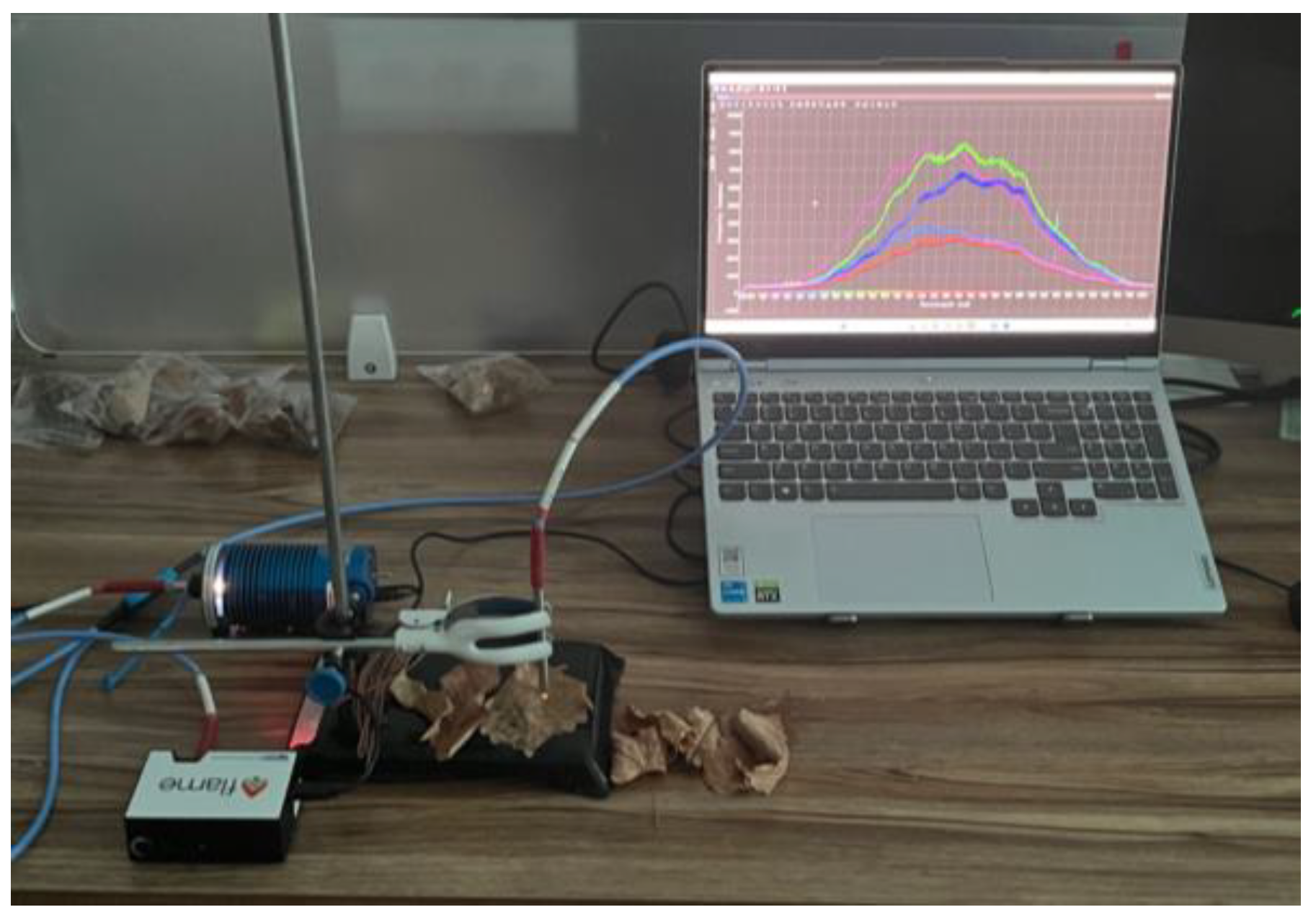
Dead fuel samples were taken from four species of trees (Mongolian oak, water willow, white birch, and larch) of the same phenology in the Harbin Urban Forestry Demonstration Base, and the sample collection method was referenced from Catchpole’s study. In order to simulate the wet state of dead combustibles in the natural environment, all samples were soaked in distilled water for 1 h, and control groups with different moisture contents of the same dead combustibles were set up by controlling the difference in the drying time of the samples. Then, the samples were measured by the Flame spectrometer of Ocean Optics, with a spectral resolution of 1 nm, combined with a “Y” type optical fiber for visible reflectance spectroscopy, and the light source used was an HL-2000 tungsten halogen lamp with a power of 5 W (Figure 2).
The spectrometer was connected to a computer, and the reflection spectra measured in real time were displayed through OceanView 2.0.8 software, and the measurement results are shown in Figure 3. From the figure, it can be seen that the intensity of the reflection spectra of the dead fuel from different tree species differed after soaking for the same time, with the highest intensity of the reflection spectra of the dead fuel material from the Mongolian oak and the lowest intensity of the reflection spectra of the dead fuel material from the larch. The peak reflectance spectra of different species are also different, such as the peak wavelength of the reflectance spectra of the dead fuel from the water willow being 641 nm, and the peak wavelength of the reflectance spectra of the dead fuel from the Mongolian oak being 696 nm. The green and blue spectra are the reflectance spectra of the same species of dead fuel, soaked for the same time and dried for different times, that is, with different moisture content. Therefore, the intensity of the reflectance spectra of the same kind of withered material with different water content is also different. The above results provide a basis for the selection of spectral bands in the actual measurement and provide the feasibility for the subsequent prediction of DFMC by multispectral imagery.
2.3. Data Acquisition and Processing
In this paper, a DJI(DJ-Innovations) M300RTK UAV was used as the UAV platform, and the multispectral camera model was an MS600Pro with six spectral bands, 450 nm, 555 nm, 660 nm, 720 nm, 750 nm, and 840 nm. The UAV was equipped with a multispectral camera and conducted an eight-day cruise photography mission at the same time and on the same route on 9 March, 10 March, 11 March, 13 March, 17 March, 18 March, 19 March, and 23 March, flying at an altitude of 40 m, with a route speed of 5.5 m/s, a camera shooting interval of 1 s, an overlap rate of 80%, a bypass overlap rate of 70%, and a shooting area of 68,339 square meters, taking a total of 5945 groups of images. Each group contained six single-band images with a resolution of 1280 × 960 and a spatial resolution of 2.88 cm. The mission lasted for 20′47″, consuming 57% of the power from two 5935 mAh batteries (Figure 4).
Using Yusense Map 2.2.3 software, the camera parameters were read from the images to complete the image internal orientation and band alignment, and the six single-band images were combined into a six-band multispectral image. Finally, the standard reflectance was read from the captured calibration gray plate images to complete the radiometric calibration (Table 1), and finally, 5945 multispectral remote-sensing images with real surface reflectance were generated (Figure 5).
Surface dead combustible material samples were collected in the field in conjunction with UAV filming, and 4 sites were selected to measure dead combustible material water content, with 15 sampling points evenly distributed at each site (Figure 6), and the sample collection methodology was referenced from Catchpole’s study.
After measuring and recording the wet weight of the samples in the field, the samples were sealed and preserved for transportation, and after drying in a drying box, the dry weight of the samples was measured and recorded, and the moisture content of the samples was calculated by the formula:
where is the wet weight of the sample and is the dry weight of the same sample. In order to correspond the captured forest surface multispectral images to the ground-collected DFMC, this paper uses inverse distance weighting [38] interpolation to populate the out-of-sampling point DFMC. The weather and measured DFMC for the experimental area on the eight days of the experiment are shown in Table 2.
2.4. K-Means
Deep-learning-based segmentation is a more widely used segmentation algorithm, such as VGGNet [39], ResNet [40], R-CNN [41], FCN [42], etc. However, these algorithms require a large amount of complex labeling information and are not suitable for the segmentation of tree trunks and shadows [43]. K-means [44] is a clustering algorithm, one of the most popular unsupervised algorithms for solving clustering problems, whose goal is to divide a given dataset into K different groups or clusters such that the similarity (or distance) between data points within the same group is as small as possible, while the similarity (or distance) between data points between different groups is as large as possible. The basic idea of the K-means algorithm is to first randomly select K points as the initial cluster centers. Then, assign each data point to the group whose cluster center is closest to it, then recalculate the cluster centers for each group, and repeat the above steps until the cluster centers no longer change or a predetermined number of iterations is reached.
The steps of the K-means algorithm are as follows:
- (1)
- First, select K points at random as the initial clustering centers;
- (2)
- For each data point, calculate its distance from the K clustering centers and assign that data point to the group in which the nearest clustering center is located;
- (3)
- For each group, recalculate its cluster center, i.e., average the coordinates of all data points within that group to obtain a new cluster center.
Repeat steps 2 and 3 until the clustering centers no longer change or a predetermined number of iterations is reached.
Therefore, the K-means unsupervised segmentation algorithm was utilized, and K was set to be 3, which enabled the clustering of tree trunks, shadows, and surface dead fuel into three distinct clusters. As a result, the segmentation of trees and shadows was realized, and the coverage of trees and shadows was removed, retaining only the multispectral image of surface dead fuels.
2.5. ConvNeXt
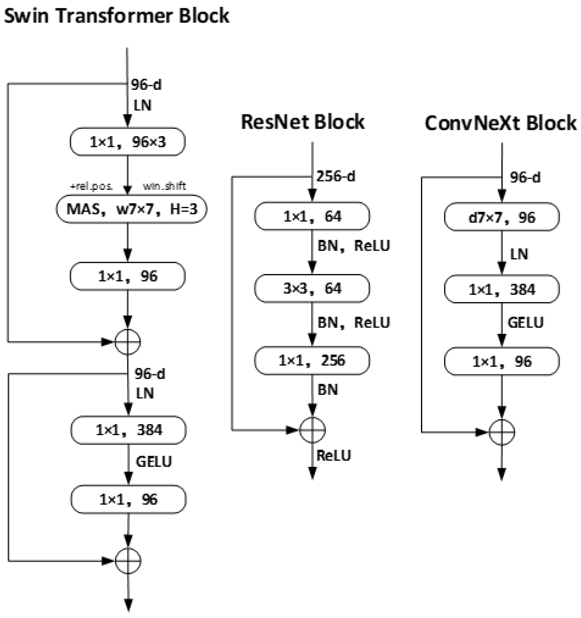
Based on the structure of Swin Transformer [45], Zhuang Liu et al. [46] changed the structure of ResNet [40] and proposed a pure convolutional neural network of ConvNeXt. After experimental demonstration in the literature, the pure convolutional network (ConvNeXt) outperformed Swin Transformer in a classification task, target detection task, and image segmentation task with the same amount of computation.
The most important feature of ConvNeXt is the change in the original ResNet structure by referring to the structure of Swin Transformer. The number of stackings in ConvNeXt is adjusted from (3, 4, 6, 3) of ResNet 50 to (3, 3, 9, 3), which reduces the number of floating point operations per second (FLOPs). ConvNeXt uses convolutional kernels of size 4 × 4 with 4 steps which constitute patchify and downsample by a factor of 4. ConvNeXt uses a depthwise convolution structure, where each convolutional kernel has a channel number of 1 and each convolutional kernel is responsible for only one channel of the input feature matrix, reducing the amount of convolutional computation by a factor of 8 to 9 compared to conventional convolution. The depthwise convolution module is moved up and the size of the convolution kernel is changed from 3 × 3 to 7 × 7, reducing the FLOPs again. The GELU activation function and layer normalization are used in the ConvNeXt Block, while the activation function and normalization layer are reduced. The block structures of ResNet, Swin Transformer, and ConvNeXt are shown in Figure 7.
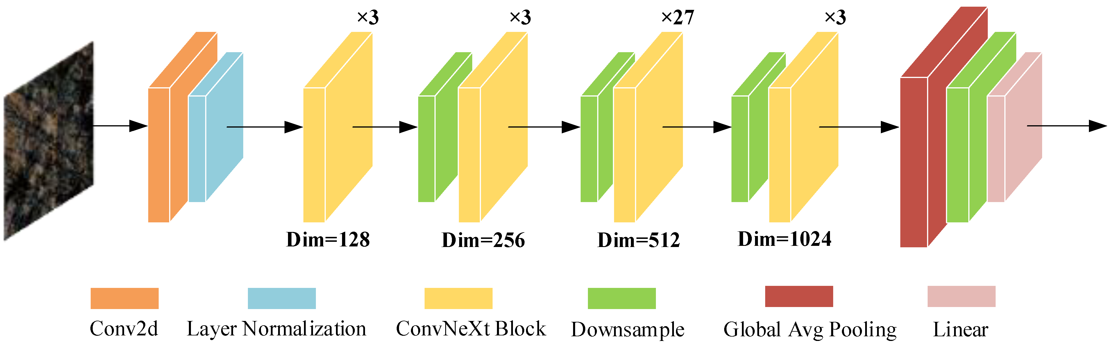
The model used in this paper is a ConvNeXt-B in a ConvNeXt network with the number of channels C = (128, 256, 512, 1024) and the number of blocks B = (3, 3, 27, 3). The size of the multispectral image in the dataset used in this paper is 256 × 256 × 6. In order to input the data into the ConvNeXt model, the number of channels in the first convolutional layer of the ConvNeXt model needs to be changed to six. After the first convolutional layer and layer normalization, the image size becomes 64 × 64 × 128, and after 3 layers of the ConvNeXt Block and depth 128, the image size becomes 64 × 64 × 128; after another downsampling, 3 layers of the ConvNeXt Block and depth 256, the image size becomes 32 × 32 × 256; again, after another downsampling, 27 layers of the ConvNeXt Block and depth 512, the image size becomes 16 × 16 × 512; then, after one downsampling, 3 layers of the ConvNeXt Block and a depth of 1024, the image size becomes 8 × 8 × 1024. The feature-image output from the convolutional layer undergoes a pooling operation in the global average pooling layer to obtain a global feature vector; after layer normalization normalizes the global feature vector, the fully connected layer maps the global feature vector to 8 output categories, outputs the confidence scores of the 8 categories, and converts the outputs to probability distributions using the Softmax function. In the backpropagation stage, the error term of the output layer is first calculated, then the gradient of the fully connected layer is calculated based on the error term and the weights of the fully connected layer, then the gradient is passed back to the global average pooling layer, and finally, passed back to the convolutional layer and the input layer to calculate the gradient of each layer and update the parameters (Figure 8).
In this paper, depending on the orientation of the UAV and the rotation angle of the multispectral camera, different views of the same area may be acquired at different time ranges. Using data-enhancement techniques, the multispectral images are randomly rotated and randomly flipped horizontally or vertically. By loading the ConvNeXt pretrained model for migration learning and then training the dataset, the first 10 epochs of training can achieve high accuracy, which not only reduces the training time, saves computational resources, and the cost of data collection, but also improves the generalization ability of the model, avoids overfitting, and makes the model more robust.
2.6. ResNeXt
ResNeXt is a deep-learning model that is a variant of ResNet [47]. It uses a new network structure called “cardinality” to improve model accuracy while maintaining computational efficiency. In ResNeXt, the feature maps in each residual block are divided into several subsets, or “cardinalities”. Each subset is then processed by a small branch network in parallel, and the outputs are merged to obtain the output of the entire residual block. This parallel processing approach improves the accuracy of the model while maintaining the computational efficiency. ResNeXt50 has a depth of 50 layers and uses bottleneck structures with 3 convolutional layers, where the 2nd convolutional layer has a kernel size of 1 × 1 to reduce computational complexity. The model also uses techniques such as batch normalization and residual connections to speed up training and improve accuracy. ResNeXt101 is a deeper and more powerful version of the ResNeXt architecture, based on the same “cardinality” concept as ResNeXt50. It has 101 layers and can achieve even higher accuracy on various computer vision tasks.
ResNeXt has shown excellent performance in many computer vision tasks, such as image classification, object detection, and semantic segmentation. It has become an important model in the deep-learning field and is widely used in practical applications.
2.7. ResNeXt101-ECA
ResNeXt101-ECA is an improved version of the ResNeXt101 model that incorporates the Efficient Channel Attention (ECA) [48] mechanism. It adopts the “cardinality” structure like ResNeXt and adds the ECA mechanism to each residual block to enhance the feature representation and generalization capabilities of the model.
The ECA mechanism can capture the inter-channel interactions more effectively and enhance the feature representation capability of the model. Unlike traditional attention mechanisms, ECA only needs to compute attention weights in local regions, greatly reducing the computational and storage overheads and improving the training and inference speed of the model.
2.8. Swin Transformer
Swin Transformer [45] is a novel Transformer architecture that has achieved great success in both natural language processing and computer vision fields. The main feature of Swin Transformer is the introduction of a hierarchical window mechanism, which enables it to handle inputs of arbitrary sizes and obtain better performance on high-resolution images.
The window mechanism of Swin Transformer is constructed based on nonoverlapping image blocks. Between each block, Swin Transformer uses cross-block connections to capture the information flow between blocks. Additionally, Swin Transformer introduces a new deep-segmentation attention mechanism to aggregate features at different scales and levels, enhancing the model’s representation power.
3. Results
3.1. K-Means Image Segmentation
The UAV platform is simple, flexible, and efficient, and is suitable for predicting the moisture content of dead forest surface fuels on a large scale. However, due to the occlusion by the forest vegetation canopy and its shadows, the forest surface images captured by the multispectral camera on board the UAV platform cannot be directly used for predicting the moisture content, and the multispectral images need to be segmented and processed to extract the spectral image information of dead surface fuels. This paper uses the unsupervised K-means algorithm to perform the clustering segmentation of UAV multispectral images with a set initial K value of 3 to segment the images into three parts: trees, shadows, and ground surface. A mask of the dead fuel part of the ground surface is generated, and the original image is mask segmented to retain only the spectral information of the dead fuel on the ground surface (Figure 9).
The 5945 multispectral images were segmented by K-means clustering to produce multispectral images containing only surface dead fuels. Part of the original tree and shadow information in the image is segmented, and some blank areas appear. In order to reduce the amount of modeling operations and increase the proportion of useful information in the image, in this paper, the image with 1280 × 960 resolution is cut out of the image with the highest gray value in the image and the resolution of 256 × 256 as the final dataset. The dataset was divided into training, validation, and test sets according to 8:1:1.
3.2. ConvNeXt Predicts DFMC
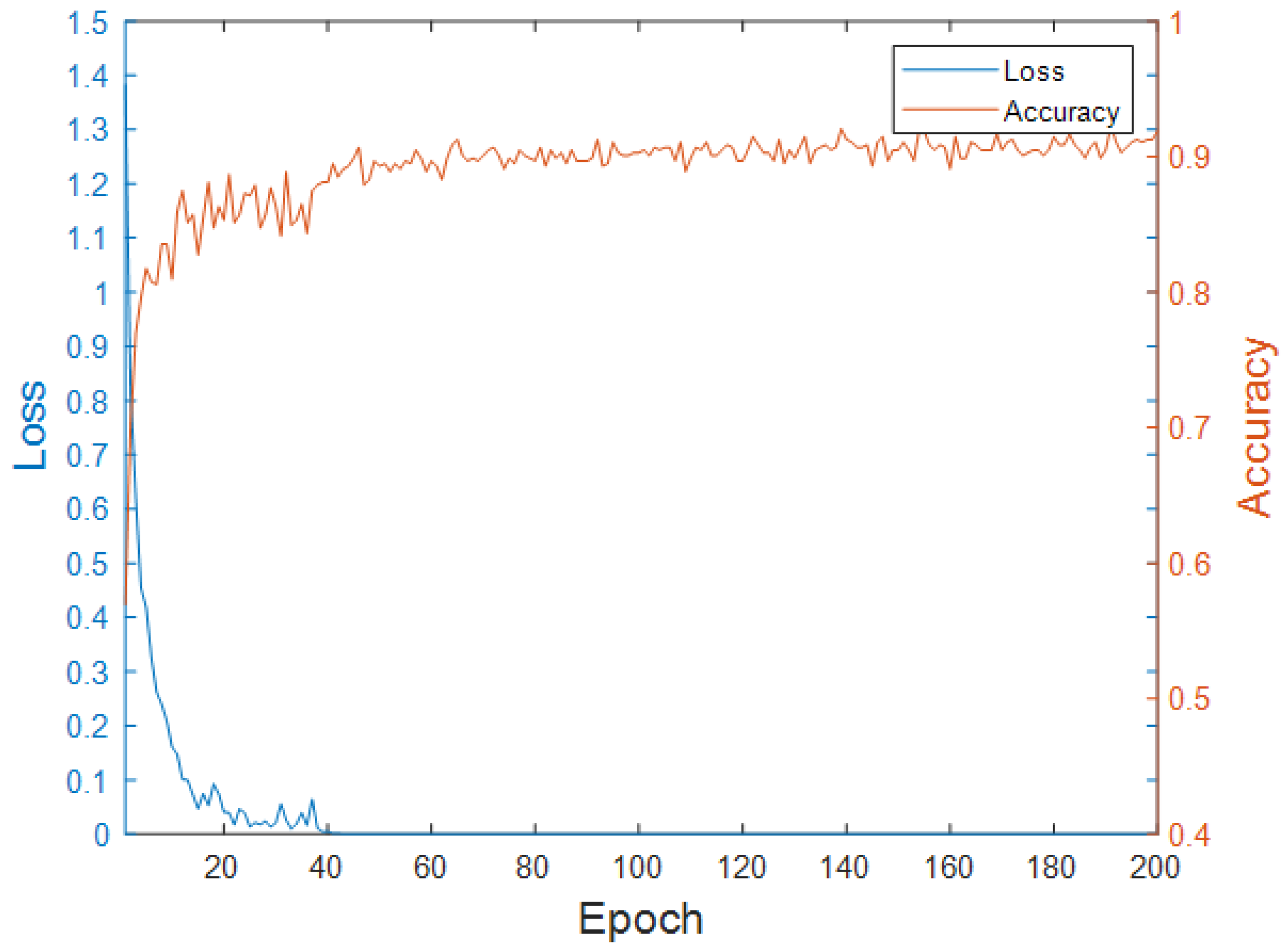
In this paper, the ConvNeXt model, which is currently the best performing model in the classification problem [46], was chosen as the model for this experiment. In total, 3985 images were used for the training set, 504 images for the validation set, and 498 images for the test set, all of which were 6-channel multispectral images. The input to the ConvNeXt model in this experiment is a 256 × 256 × 6 image, which is downsampled once by a convolutional layer of size 4 × 4 and layout 4, turning the height and width of the image into 1/4 of its original size, and then passed through four stages in turn; each stage is composed of a series of ConvNeXt blocks, and the ratio of the four stages is 3:3:9:9. The output of the last stage is subjected to global average pooling, layer normalization, and finally, the confidence scores of the eight categories are output after a fully connected layer, and the output is transformed into a probability distribution using the Softmax function. The experimental model was trained using an AdamW optimizer with an initial learning rate of 0.0001. In total, 200 epochs were trained and the model with the highest accuracy was saved as the best model, with the final model having an accuracy of 92.26% (Figure 10).
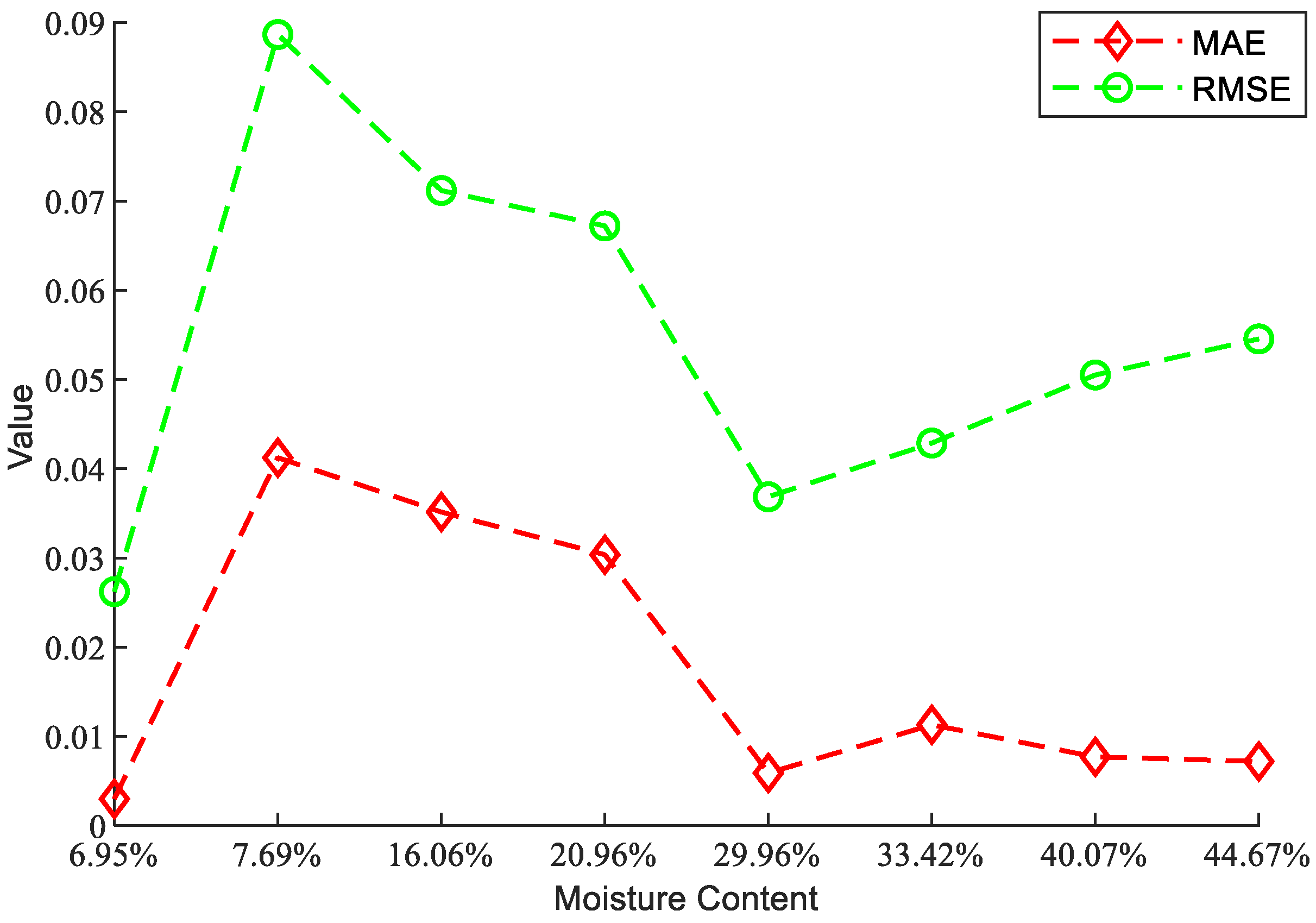
After the training was completed, this paper used a test set to evaluate the prediction effect, using the mean absolute error (MAE) and root mean square error (RMSE) as the evaluation metrics.
where is the true value, is the predicted value, and n is the number of samples. The smaller the MAE and RMSE values, the smaller the error between the true and predicted values, and the better the prediction (Figure 11).
The ConvNeXt model has an MAE of 1.54% and an RMSE of 5.45% for the predicted results on the test set.
A multispectral camera mounted on a UAV was used to capture 68,339 square meters of forest surface multispectral images over the study area. The multispectral image was subjected to K-means segmentation to remove the effects of trees and shadows, and the trained ConvNeXt model was used to predict the surface DFMC in the study area, and the visualization results are shown in Figure 12.
4. Discussion
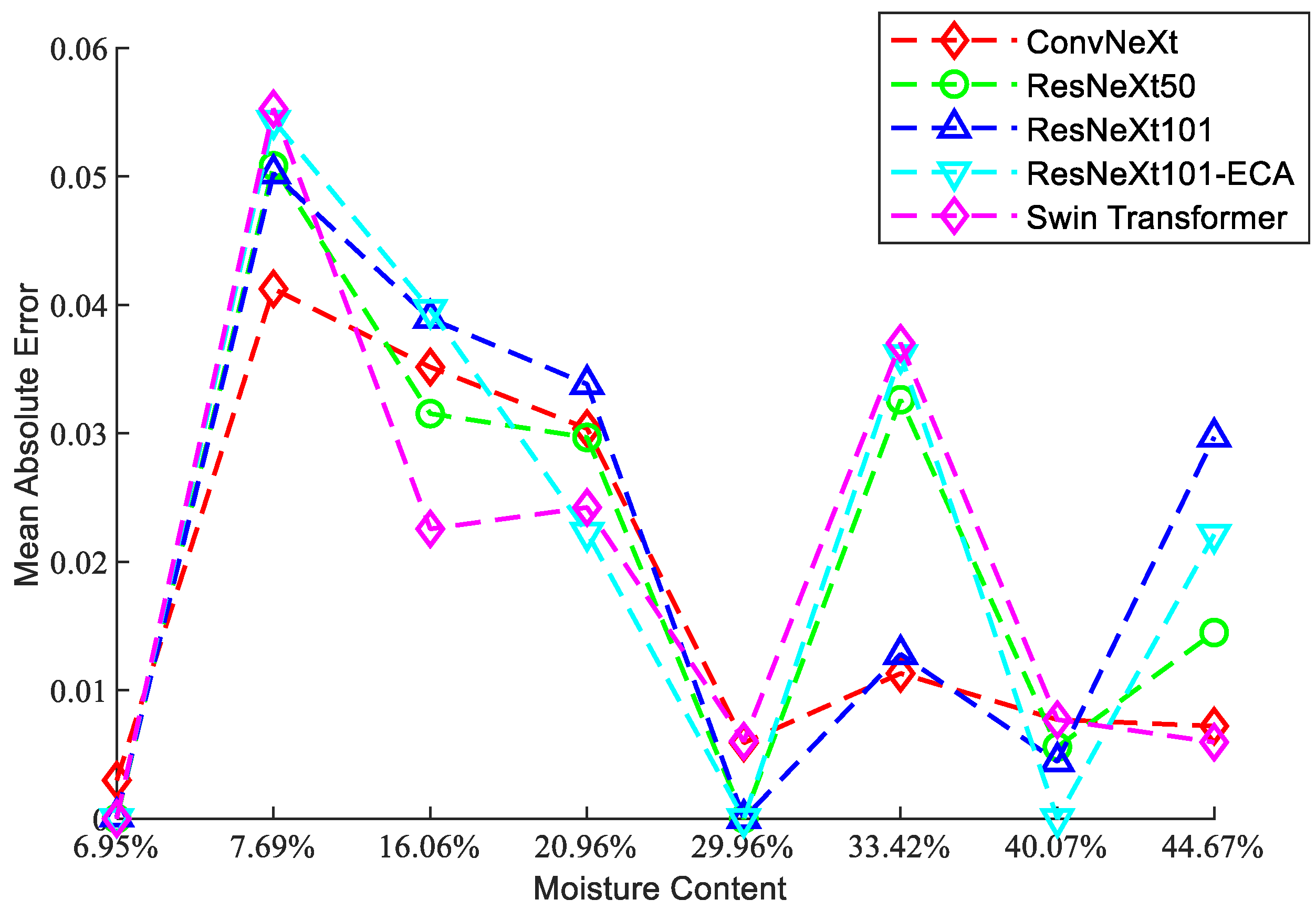
To evaluate the performance of neural networks for predicting DFMC, four convolutional neural network models were used, ConvNeXt, ResNeXt50, ResNeXt101, ResNeXt101-ECA (ResNeXt101 model with integrated ECA channel attention module), and one Transformer model (Swin Transformer); the five models are outstanding in the current image vision field. Training was performed on the dataset produced in this paper, all using the AdamW optimizer with an initial learning rate of 0.0001. In total, 200 epochs were trained, and the model with the highest accuracy was saved as the best model (Figure 13).
Table 3 shows the predictions of the five models on the test set for DFMC. As can be seen from the table, the model used in this paper (ConvNeXt) predicts a 2.68% reduction in the MAE and 1.33% reduction in the RMSE for DFMC compared to the Swin Transformer, a 30.19% reduction in the MAE and a 12.09% reduction in the RMSE for DFMC compared to the ResNeXt50, a reduction in the MAE by 44.16% and RMSE by 18.39% compared to the ResNeXt101-ECA-predicted DFMC, and a reduction in the MAE by 39.70% and RMSE by 23.43% compared to the ResNeXt101-predicted DFMC. All models have an MAE below 3% and RMSE below 7% in predicting DFMC on the test set, and the best performing ConvNeXt model has a 92.26% accuracy, 1.54% MAE, and 5.45% RMSE in predicting DFMC on the test set. The results showed that, on a forest area of 68,339 square meters, the use of UAV to capture ground-level multispectral images, combined with ground sampling of DFMC, can accurately predict forest surface DFMC through the training of a deep-learning model in this study. This provides a new method for predicting forest surface DFMC over large areas.
5. Conclusions
This paper presents a new method for predicting the DFMC of forest land surface based on UAV remote sensing. The simple, flexible, efficient, and time-sensitive features of the UAV platform are utilized to carry a multispectral camera to acquire high-resolution multispectral images of the forest surface over a large area in a short period of time. K-means clustering segmentation was performed on the multispectral images to obtain 5945 multispectral images containing only dead combustible material on the forest floor, which were made into a dataset together with the actual moisture content measured by the weighing method to provide usable data for subsequent research on the UAV multispectral prediction of DFMC. The dataset was trained by the ConvNeXt deep-learning model to evaluate the performance of predicting DFMC from multispectral images. The results showed that the ConvNeXt model predicts DFMC with a 92.26% accuracy, 1.54% MAE, and 5.45% RMSE on the test set, achieving an accurate prediction of DFMC over a large area based on multispectral images of the UAV forest floor. Future experiments will be conducted on a larger scale and for a longer period in forest areas such as the Maoer Mountains in northeast China to enrich the number and variety of datasets in order to improve the generalizability and accuracy of the model.
Author Contributions
Conceptualization, J.X. and C.W.; methodology, J.X. and C.W.; software, C.W. and J.G.; validation, J.X., C.W. and Z.C.; formal analysis, C.W., J.G. and Z.C.; investigation, Y.L. and X.C.; resources, C.W. and H.W.; data curation, Y.L. and H.W.; writing—original draft preparation, C.W.; writing—review and editing, J.X. and C.W.; visualization, Z.C. and X.C.. All authors have read and agreed to the published version of the manuscript.
Funding
National Natural Science Foundation of China (32371864).
Institutional Review Board Statement
Not applicable.
Informed Consent Statement
Not applicable.
Data Availability Statement
The data presented in this study are available on request from the corresponding author.
Conflicts of Interest
The authors declare no conflict of interest.
References
- Souza, C.R.; Maia, V.A.; Mariano, R.F.; de Souza, F.C.; de Carvalho Araújo, F.; de Paula, G.G.; de Oliveira Menino, G.C.; Coelho, P.A.; Santos, P.F.; Morel, J.D. Tropical forests in ecotonal regions as a carbon source linked to anthropogenic fires: A 15-year study case in Atlantic forest—Cerrado transition zone. For. Ecol. Manag. 2022, 519, 120326. [Google Scholar] [CrossRef]
- Ministry of Environment; Forest and Climate Change Government of India; World Bank. Strengthening Forest Fire Management in India; World Bank: Washington, WA, USA, 2018. [Google Scholar]
- Song, R.; Wang, T.; Han, J.; Xu, B.; Ma, D.; Zhang, M.; Li, S.; Zhuang, B.; Li, M.; Xie, M. Spatial and temporal variation of air pollutant emissions from forest fires in China. Atmos. Environ. 2022, 281, 119156. [Google Scholar] [CrossRef]
- Sannigrahi, S.; Pilla, F.; Maiti, A.; Bar, S.; Bhatt, S.; Zhang, Q.; Keesstra, S.; Cerda, A. Examining the status of forest fire emission in 2020 and its connection to COVID-19 incidents in West Coast regions of the United States. Environ. Res. 2022, 210, 112818. [Google Scholar] [CrossRef]
- Zong, X.; Tian, X.; Liu, J. A Fire Regime Zoning System for China. Front. For. Glob. Change 2021, 4, 717499. [Google Scholar] [CrossRef]
- Kong, J.-J.; Yang, J.; Bai, E. Long-term effects of wildfire on available soil nutrient composition and stoichiometry in a Chinese boreal forest. Sci. Total Environ. 2018, 642, 1353–1361. [Google Scholar] [CrossRef]
- Zhou, Q.; Zhang, H.; Wu, Z. Effects of Forest Fire Prevention Policies on Probability and Drivers of Forest Fires in the Boreal Forests of China during Different Periods. Remote Sens. 2022, 14, 5724. [Google Scholar] [CrossRef]
- Nelson, R.M., Jr. Prediction of diurnal change in 10-h fuel stick moisture content. Can. J. For. Res. 2000, 30, 1071–1087. [Google Scholar] [CrossRef]
- Zhao, F.; Liu, Y.; Shu, L. Change in the fire season pattern from bimodal to unimodal under climate change: The case of Daxing’anling in Northeast China. Agric. For. Meteorol. 2020, 291, 108075. [Google Scholar] [CrossRef]
- Stephens, S.L.; Burrows, N.; Buyantuyev, A.; Gray, R.W.; Keane, R.E.; Kubian, R.; Liu, S.; Seijo, F.; Shu, L.; Tolhurst, K.G. Temperate and boreal forest mega-fires: Characteristics and challenges. Front. Ecol. Environ. 2014, 12, 115–122. [Google Scholar] [CrossRef]
- Ceccato, P.; Leblon, B.; Chuvieco, E.; Flasse, S.; Carlson, J. Estimation of live fuel moisture content. In Wildland Fire Danger Estimation and Mapping: The Role of Remote Sensing Data; World Scientific: Singapore, 2003; pp. 63–90. [Google Scholar]
- Catchpole, E.A.; Catchpole, W.R.; Viney, N.R.; McCaw, W.L.; Marsden-Smedley, J.B. Estimating fuel response time and predicting fuel moisture content from field data. Int. J. Wildland Fire 2001, 10, 215–222. [Google Scholar] [CrossRef]
- Nelson, R.M.; Hiers, J.K. The influence of fuelbed properties on moisture drying rates and timelags of longleaf pine litter. Can. J. For. Res. 2008, 38, 2394–2404. [Google Scholar] [CrossRef]
- Nelson, R.M., Jr. A method for describing equilibrium moisture content of forest fuels. Can. J. For. Res. 1984, 14, 597–600. [Google Scholar] [CrossRef]
- Yu, H.; Shu, L.; Yang, G.; Deng, J. Comparison of vapour-exchange methods for predicting hourly twig fuel moisture contents of larch and birch stands in the Daxinganling Region, China. Int. J. Wildland Fire 2021, 30, 462–466. [Google Scholar] [CrossRef]
- Matthews, S. A process-based model of fine fuel moisture. Int. J. Wildland Fire 2006, 15, 155–168. [Google Scholar] [CrossRef]
- Zhao, L.; Yebra, M.; van Dijk, A.I.; Cary, G.J.; Matthews, S.; Sheridan, G. The influence of soil moisture on surface and sub-surface litter fuel moisture simulation at five Australian sites. Agric. For. Meteorol. 2021, 298, 108282. [Google Scholar] [CrossRef]
- Anderson, H.E. Predicting Equilibrium Moisture Content of Some Foliar Forest Litter in the Northern Rocky Mountains; US Department of Agriculture, Forest Service, Intermountain Research Station: Ogden, UT, USA, 1990; Volume 429. [Google Scholar]
- Van der Kamp, D.; Moore, R.; McKendry, I. A model for simulating the moisture content of standardized fuel sticks of various sizes. Agric. For. Meteorol. 2017, 236, 123–134. [Google Scholar] [CrossRef]
- Matthews, S. Dead fuel moisture research: 1991–2012. Int. J. Wildland Fire 2014, 23, 78–92. [Google Scholar] [CrossRef]
- Alves, M.; Batista, A.; Soares, R.; Ottaviano, M.; Marchetti, M. Fuel moisture sampling and modeling in Pinus elliottii Engelm. plantations based on weather conditions in Paraná-Brazil. Iforest-Biogeosciences For. 2009, 2, 99. [Google Scholar] [CrossRef]
- Sharples, J.J.; McRae, R.H.; Weber, R.; Gill, A.M. A simple index for assessing fuel moisture content. Environ. Model. Softw. 2009, 24, 637–646. [Google Scholar] [CrossRef]
- de Dios, V.R.; Fellows, A.W.; Nolan, R.H.; Boer, M.M.; Bradstock, R.A.; Domingo, F.; Goulden, M.L. A semi-mechanistic model for predicting the moisture content of fine litter. Agric. For. Meteorol. 2015, 203, 64–73. [Google Scholar] [CrossRef]
- Bilgili, E.; Coskuner, K.A.; Usta, Y.; Goltas, M. Modeling surface fuels moisture content in Pinus brutia stands. J. For. Res. 2019, 30, 577–587. [Google Scholar] [CrossRef]
- Masinda, M.M.; Li, F.; Liu, Q.; Sun, L.; Hu, T. Prediction model of moisture content of dead fine fuel in forest plantations on Maoer Mountain, Northeast China. J. For. Res. 2021, 32, 2023–2035. [Google Scholar] [CrossRef]
- Wittich, K.-P. A single-layer litter-moisture model for estimating forest-fire danger. Meteorol. Z. 2005, 14, 157–164. [Google Scholar] [CrossRef] [PubMed]
- Qu, Z.; Min, Y.; Zhao, L.; Hu, H. Study on the predicted model of forest fuel moisture. In Proceedings of 2010 International Conference on Electrical and Control Engineering, Wuhan, China, 25–27 June 2010; pp. 2170–2173. [Google Scholar]
- Fan, C.; He, B. A Physics-Guided Deep Learning Model for 10-h Dead Fuel Moisture Content Estimation. Forests 2021, 12, 933. [Google Scholar] [CrossRef]
- Fan, C.; He, B.; Yin, J.; Chen, R. Regional estimation of dead fuel moisture content in southwest China based on a practical process-based model. Int. J. Wildland Fire 2023, 32, 1148–1161. [Google Scholar] [CrossRef]
- Peng, B.; Zhang, J.; Xing, J.; Liu, J. Distribution prediction of moisture content of dead fuel on the forest floor of Maoershan national forest, China using a LoRa wireless network. J. For. Res. 2022, 33, 899–909. [Google Scholar] [CrossRef]
- Quan, X.; He, B.; Li, X.; Liao, Z. Retrieval of grassland live fuel moisture content by parameterizing radiative transfer model with interval estimated LAI. IEEE J. Sel. Top. Appl. Earth Obs. Remote Sens. 2015, 9, 910–920. [Google Scholar] [CrossRef]
- Yebra, M.; Dennison, P.E.; Chuvieco, E.; Riaño, D.; Zylstra, P.; Hunt, E.R., Jr.; Danson, F.M.; Qi, Y.; Jurdao, S. A global review of remote sensing of live fuel moisture content for fire danger assessment: Moving towards operational products. Remote Sens. Environ. 2013, 136, 455–468. [Google Scholar] [CrossRef]
- Nieto, H.; Aguado, I.; Chuvieco, E.; Sandholt, I. Dead fuel moisture estimation with MSG–SEVIRI data. Retrieval of meteorological data for the calculation of the equilibrium moisture content. Agric. For. Meteorol. 2010, 150, 861–870. [Google Scholar] [CrossRef]
- Nolan, R.H.; de Dios, V.R.; Boer, M.M.; Caccamo, G.; Goulden, M.L.; Bradstock, R.A. Predicting dead fine fuel moisture at regional scales using vapour pressure deficit from MODIS and gridded weather data. Remote Sens. Environ. 2016, 174, 100–108. [Google Scholar] [CrossRef]
- Dragozi, E.; Giannaros, T.M.; Kotroni, V.; Lagouvardos, K.; Koletsis, I. Dead Fuel Moisture Content (DFMC) Estimation Using MODIS and Meteorological Data: The Case of Greece. Remote Sens. 2021, 13, 4224. [Google Scholar] [CrossRef]
- Quan, X.; He, B.; Yebra, M.; Yin, C.; Liao, Z.; Li, X. Retrieval of forest fuel moisture content using a coupled radiative transfer model. Environ. Model. Softw. 2017, 95, 290–302. [Google Scholar] [CrossRef]
- Sun, C.; Huang, C.; Zhang, H.; Chen, B.; An, F.; Wang, L.; Yun, T. Individual Tree Crown Segmentation and Crown Width Extraction From a Heightmap Derived From Aerial Laser Scanning Data Using a Deep Learning Framework. Front. Plant Sci. 2022, 13, 914974. [Google Scholar] [CrossRef] [PubMed]
- Lu, G.Y.; Wong, D.W. An adaptive inverse-distance weighting spatial interpolation technique. Comput. Geosci. 2008, 34, 1044–1055. [Google Scholar] [CrossRef]
- Simonyan, K.; Zisserman, A. Very deep convolutional networks for large-scale image recognition. arXiv 2014, arXiv:1409.1556. [Google Scholar]
- He, K.; Zhang, X.; Ren, S.; Sun, J. Deep residual learning for image recognition. In Proceedings of the IEEE Conference on Computer Vision and Pattern Recognition, Las Vegas, NV, USA, 26 June–1 July 2016; pp. 770–778. [Google Scholar]
- Girshick, R.; Donahue, J.; Darrell, T.; Malik, J. Rich feature hierarchies for accurate object detection and semantic segmentation. In Proceedings of the IEEE Conference on Computer Vision and Pattern Recognition, Washington, DC, USA, 23–28 June 2014; pp. 580–587. [Google Scholar]
- Long, J.; Shelhamer, E.; Darrell, T. Fully convolutional networks for semantic segmentation. In Proceedings of the IEEE Conference on Computer Vision and Pattern Recognition, Boston, MA, USA, 7–12 June 2015; pp. 3431–3440. [Google Scholar]
- Yun, T.; Jiang, K.; Hou, H.; An, F.; Chen, B.; Jiang, A.; Li, W.; Xue, L. Rubber Tree Crown Segmentation and Property Retrieval Using Ground-Based Mobile LiDAR after Natural Disturbances. Remote Sens. 2019, 11, 903. [Google Scholar] [CrossRef]
- Hartigan, J.A.; Wong, M.A. Algorithm AS 136: A k-means clustering algorithm. J. R. Stat. Society. Ser. C (Appl. Stat.) 1979, 28, 100–108. [Google Scholar] [CrossRef]
- Liu, Z.; Lin, Y.; Cao, Y.; Hu, H.; Wei, Y.; Zhang, Z.; Lin, S.; Guo, B. Swin transformer: Hierarchical vision transformer using shifted windows. In Proceedings of the IEEE/CVF International Conference on Computer Vision, Nashville, TN, USA, 20–25 June 2021; pp. 10012–10022. [Google Scholar]
- Liu, Z.; Mao, H.; Wu, C.-Y.; Feichtenhofer, C.; Darrell, T.; Xie, S. A convnet for the 2020s. In Proceedings of the IEEE/CVF Conference on Computer Vision and Pattern Recognition, New Orleans, LA, USA, 18–24 June 2022; pp. 11976–11986. [Google Scholar]
- Xie, S.; Girshick, R.; Dollár, P.; Tu, Z.; He, K. Aggregated residual transformations for deep neural networks. In Proceedings of the IEEE Conference on Computer Vision and Pattern Recognition, Honolulu, HI, USA, 21–26 July 2017; pp. 1492–1500. [Google Scholar]
- Wang, Q.; Wu, B.; Zhu, P.; Li, P.; Zuo, W.; Hu, Q. ECA-Net: Efficient channel attention for deep convolutional neural networks. In Proceedings of the IEEE/CVF Conference on Computer Vision and Pattern Recognition, Seattle, WA, USA, 13–19 June 2020; pp. 11534–11542. [Google Scholar]
Figure 1.
Study area.

Figure 2.
Experiment of reflectance spectroscopy measurement of apoplast.

Figure 3.
Visible reflectance spectra of dead fuel.

Figure 4.
Diagram of the data acquisition equipment. In figure (a), the UAV is flying a mission over the study area; figure (b) is the M300RTK UAV used in this paper; figure (c) is the MS600PRO multispectral camera on board the UAV platform; figure (d) is a six-band image of the calibration gray plate taken with a multispectral camera.

Figure 5.
False color image synthesized from multispectral images of the forest floor. The left image was taken on 13 March and shows snow in the white part of the image; the picture on the right was taken on 19 March, the snow has all melted, the light outside is strong, the white part of the picture is the glare from the tree canopy.

Figure 6.
Diagram of the UAV’s flight path and dead combustible sample sampling points. The green line in the left figure is the flight route of the UAV, the part surrounded by the red dotted line in the right figure is the dead combustible sample sampling area, and the 15 red dots are the dead combustible sample sampling points.

Figure 7.
Block design of ResNet, Swin Transformer, and ConvNeXt.

Figure 8.
Brief structure of ConvNeXt.

Figure 9.
K-means segmented images. (a,d,g) are surface pseudocolor images; (b,e,h) are multispectral images of tree masks segmented by K-means; (c,f,i) are multispectral images of surface dead fuel masks segmented by K-means.
Figure 9.
K-means segmented images. (a,d,g) are surface pseudocolor images; (b,e,h) are multispectral images of tree masks segmented by K-means; (c,f,i) are multispectral images of surface dead fuel masks segmented by K-means.

Figure 10.
Accuracy results of ConvNeXt model training.

Figure 11.
ConvNeXt model prediction results on the test set.

Figure 12.
Distribution of forest surface DFMC. The red part is mainly larch woodland with high DFMC values; the dark blue part is mainly buff willow woodland with low DFMC values; and the green part in the middle is mainly birch and Mongolian oak woodland.
Figure 12.
Distribution of forest surface DFMC. The red part is mainly larch woodland with high DFMC values; the dark blue part is mainly buff willow woodland with low DFMC values; and the green part in the middle is mainly birch and Mongolian oak woodland.

Figure 13.
Plot of prediction results of five deep-learning models on the test set.


Table 1.
Reflectance of six wavelengths of light shining on the calibration gray plate.
| Wavelength | 450 nm | 555 nm | 660 nm | 720 nm | 750 nm | 840 nm |
| Reflectance | 0.65 | 0.62 | 0.61 | 0.61 | 0.60 | 0.59 |
Table 2.
Weather conditions and measured DFMC in the experimental area.
| Date | Maximum Temperature | Minimum Temperature | Weather | DFMC |
|---|---|---|---|---|
| 9 March | 10 °C | −2 °C | Cloudy | 40.07% |
| 10 March | 14 °C | −4 °C | Cloudy | 29.97% |
| 11 March | 3 °C | −8 °C | Sunny | 16.07% |
| 13 March | 0 °C | −9 °C | Sunny | 7.69% |
| 17 March | 5 °C | −6 °C | Sunny | 44.67% |
| 18 March | 9 °C | −4 °C | Cloudy | 33.42% |
| 19 March | 14 °C | −1 °C | Cloudy | 20.96% |
| 23 March | 1 °C | −7 °C | Cloudy | 6.95% |
Table 3.
Five model DFMC prediction results.
| Model | MAE | RMSE |
|---|---|---|
| ConvNeXt | 1.54% | 5.45% |
| Swin Transformer | 1.95% | 5.52% |
| ResNeXt50 | 2.00% | 6.11% |
| ResNeXt101-ECA | 2.22% | 6.45% |
| ResNeXt101 | 2.15% | 6.73% |
Disclaimer/Publisher’s Note: The statements, opinions and data contained in all publications are solely those of the individual author(s) and contributor(s) and not of MDPI and/or the editor(s). MDPI and/or the editor(s) disclaim responsibility for any injury to people or property resulting from any ideas, methods, instructions or products referred to in the content. |
© 2023 by the authors. Licensee MDPI, Basel, Switzerland. This article is an open access article distributed under the terms and conditions of the Creative Commons Attribution (CC BY) license (https://creativecommons.org/licenses/by/4.0/).
Share and Cite
MDPI and ACS Style
Xing, J.; Wang, C.; Liu, Y.; Chao, Z.; Guo, J.; Wang, H.; Chang, X. UAV Multispectral Imagery Predicts Dead Fuel Moisture Content. Forests 2023, 14, 1724. https://0-doi-org.brum.beds.ac.uk/10.3390/f14091724
AMA Style
Xing J, Wang C, Liu Y, Chao Z, Guo J, Wang H, Chang X. UAV Multispectral Imagery Predicts Dead Fuel Moisture Content. Forests. 2023; 14(9):1724. https://0-doi-org.brum.beds.ac.uk/10.3390/f14091724
Chicago/Turabian StyleXing, Jian, Chaoyong Wang, Ying Liu, Zibo Chao, Jiabo Guo, Haitao Wang, and Xinfang Chang. 2023. "UAV Multispectral Imagery Predicts Dead Fuel Moisture Content" Forests 14, no. 9: 1724. https://0-doi-org.brum.beds.ac.uk/10.3390/f14091724
Note that from the first issue of 2016, this journal uses article numbers instead of page numbers. See further details here.