Article

Quantifying the Impact of Different Ways to Delimit Study Areas on the Assessment of Species Diversity of an Urban Forest

1
Key Laboratory of Protection and Developmental Utilization of Tropical Crop Germplasm Resources of Ministry of Education, Hainan University, Haikou 570228, China
2
College of Horticulture and Landscape Architecture, Hainan University, Haikou 570228, China
3
Ministry of Education Key Laboratory for Earth System Modeling, Center for Earth System Science, Tsinghua University, Beijing 100084, China
4
Joint Center for Global Change Studies (JCGCS), Beijing 100875, China
*
Authors to whom correspondence should be addressed.
Submission received: 2 November 2015 / Revised: 25 January 2016 / Accepted: 28 January 2016 / Published: 15 February 2016

Abstract

:
Assessing the species diversity of an urban forest is important for understanding its structure and functions, but the result can be affected by sampling methods, times, and delimitations of the study area. In this study, we examined the influence of different ways to delimit boundaries of urban areas on the assessment of species diversity of urban forests through a case study conducted in Haikou, China. We surveyed the species diversity of the urban forest in Haikou twice using the same sampling protocol but two commonly used delimitations of the urban area. The two surveys produced significantly different estimates of species richness of the urban forest. Recorded species richness was 228 (144 woody and 84 herbaceous species) and 303 (164 woody and 139 herbaceous species) for the first and the second survey, respectively. The rarefaction analysis indicated that species richness of woody plants recorded in the two surveys could converge by doubling the sample size, but species richness of herbaceous plants was significantly different between the two surveys at the 95% confidence interval even at three times the original sample size. The value of the Simpson dissimilarity index between the two surveys was 0.417 and 0.357 for woody and herbaceous plants respectively, which implied noticeable dissimilarity of species compositions of plant assemblages in the two areas. We concluded that the assessment of biodiversity of an urban forest can be affected significantly by how the boundary of an urban area is defined. Caution should be taken when comparing species diversities of urban forests reported in different studies, especially when richness measures are used.

1. Introduction

Humans live in an increasingly urbanized world. More than 50% of the global population currently lives in urban areas and the number will increase to 66% by 2050 [1]. It is predicted that global urban land cover will increase by 1.2 million km2 by 2030 and will directly impact 1.8% of all biodiversity hotspot areas [2]. Because of these expected changes, conserving and enhancing urban biodiversity has become an increasingly important task. Conserving vegetation in urban areas can improve conservation efforts in natural areas and contribute to urban residents’ well-being in multiple ways [3,4]. It can also help to increase public awareness of the importance of biodiversity conservation since more than half of the global population experiences “nature” primarily in urban areas [5]. The urban forest, defined as the sum of all woody and associated vegetation in and around dense human settlements [6], thus needs to be managed by the urban forestry department to enhance urban biodiversity. As the first step to develop sound management practices, information on species diversity of urban forests needs to be collected.
Extensive studies on species diversity of urban forests in different parts of the world have been conducted since the 1970s [7,8,9,10,11]. These studies show that urban forests contain considerably diverse species [12]. In some cities, species diversities of urban forests are even higher than surrounding natural environments [13]. While existing studies lead to a better understanding of the general pattern of species diversity of urban forests, there are concerns about the factors influencing the study results. Pyšek [14] notes that sampling methods, research durations, and delimitations of the study area all affect the results of urban vegetation surveys. For example, Nowak et al. [15] evaluated the influence of number and size of sample plots on sampling the tree populations in cities and found that the relative standard error could be reduced by increasing the number and size of sample plots. They also suggested that a sample of 150 to 200 plots (0.4 ha) was a reasonable sample size for sampling urban forests [15]. Alvarez et al. [16] compared the results of using simple and stratified random sampling methods in an urban forest inventory in Piracicaba, Brazil, and found that the simple random sampling method performed better in their study. Besides sampling method, time scale is also a strong influencing factor. Tait et al. [17] found an increasing trend in plant diversity in Adelaide, Australia in the first 20 years of settlement. The trend gradually leveled off, however, as the study duration (1836–2002) increased.
In discussions of factors that could contribute to variation among assessments of species diversity of urban forests, different ways of defining the boundaries of urban areas is mentioned least often. Researchers have long noted the lack of a uniform definition of the term “urban area” and suggested adopting a standardized definition [18]. A recent review, however, shows that the indicators used to define urban areas still vary significantly (e.g., total population size, administrative boundary, population density, impervious surface area, built structures) [19]. Positing the existence of uncertain delimitations of the study area in studies of urban forests’ species diversities naturally leads to the question: Are species diversities of urban forests obtained by studies that use different delimitations of urban boundaries comparable? The answer to this question will affect our efforts to produce generalized knowledge and theories in urban forestry.
Despite the concerns about this issue, there have been no empirical studies to date that attempt to quantify the influence of delimitations of urban areas on estimates of species diversity of urban forests. This study examines the effect of using two different delimitations of urban areas through a case study in Haikou, China. We ask the following questions: (1) Do different delimitations of urban boundaries affect the assessment of species diversity of an urban forest? (2) Why do different delimitations lead to different results?

2. Materials and Methods
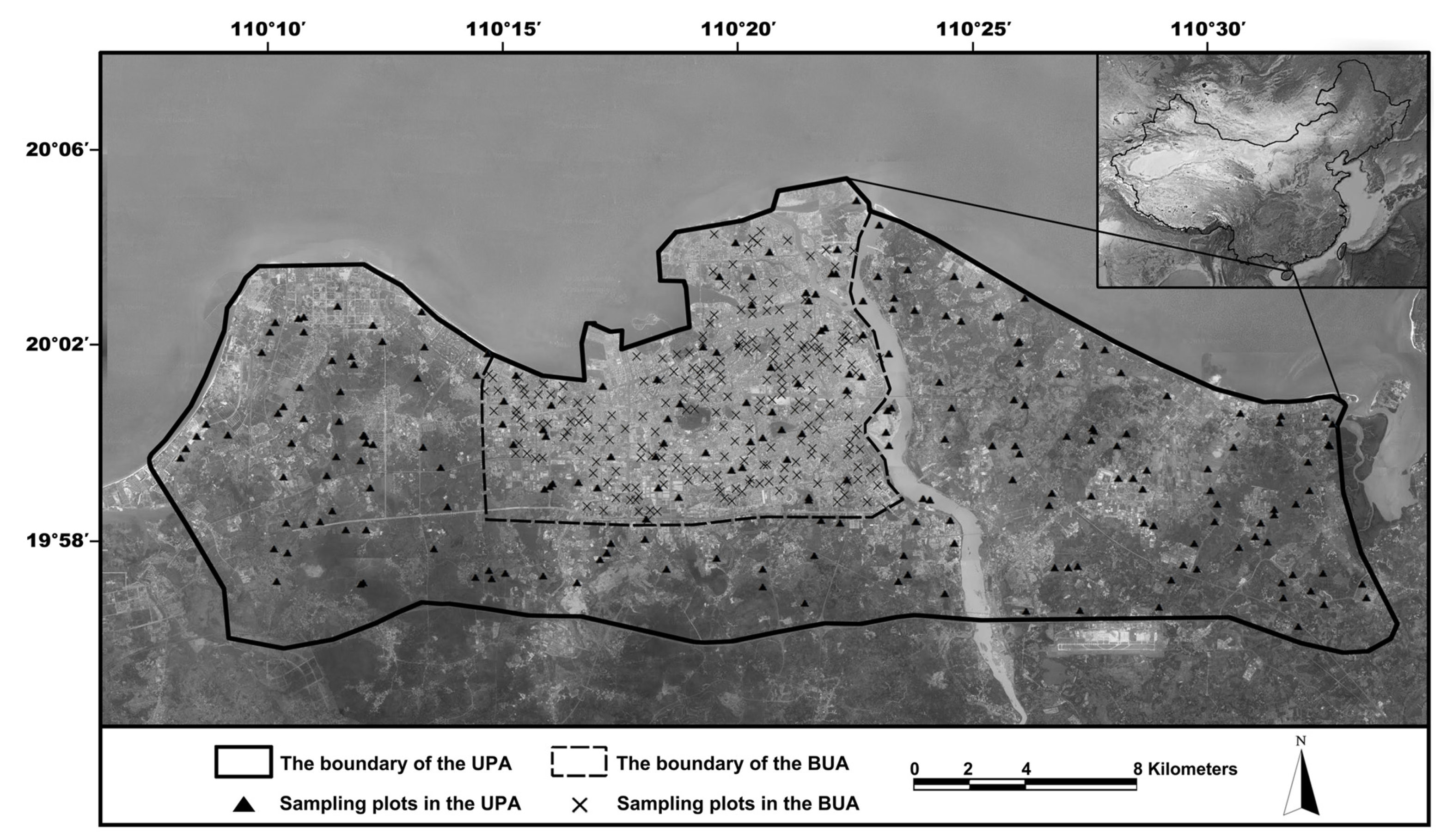
2.1. Study Area

Haikou, the largest city on Hainan Island in the South China Sea, has an administrative area of 2305 km2, roughly bounded in a zone between 110°10′ E to 110°41′ E and 19°32′ N to 20°05′ N. Haikou has a tropical monsoon climate with an annual average precipitation of 1639 mm and annual average temperature of 23.8 °C. The population was 2.1 million in 2012 [20]. The main vegetation types of Haikou are subtropical evergreen forests [21].

2.2. Field Surveys

The two field surveys were conducted by following the same sampling protocol but using different delimitations for the study areas: (1) the built-up area (BUA) delineated from the satellite image; (2) the urban area specified in the master plan of the city (urban planning area or UPA). Both delimitations have frequently been used in urban vegetation studies [22,23,24,25]. The total areas of BUA and UPA were 123.6 km2 and 507 km2, respectively (Figure 1).
Figure 1. Map showing the boundaries of the built-up area (BUA) and the urban planning area (UPA) and locations of sampling plots.
Forests 07 00042 g001
The first field survey was conducted inside the UPA in October 2012. The second survey was conducted inside the BUA in March 2013. Due to the short time span between the two surveys and the lack of significant urban development during this time period, we assumed that the species composition of urban forest in Haikou stayed roughly the same. Each time a total of 235 sample plots were laid on Google Earth (GE) randomly by first using ArcGIS 10.0 software (ESRI, Redland, CA, USA) to produce the point layer and then outputted to GE as a KML (Keyhole Markup Language) file. We adopted this sample size following the recommendation of Nowak et al. [15]. Since our goal was to examine the influence of sampling design on urban forestry studies but not to conduct a thorough investigation of all plant species in Haikou, we used this minimum sample size with 35 additional sample plots in case some plots were inaccessible.
On the ground, the field crew used print-outs of high-resolution GE images and handheld GPS units to locate the centers of sample plots. Once the center was located, the crew set up a circular plot with a radius of 12 m, resulting in a plot area of 450 m2. The crew first recorded coordinates and the dominant type of land use in the sample plot. All plant species inside the plot were then identified and recorded. Identifications were made by referring to Flora of Hainan [26], Flora of Guangdong [27], and Inventory of Plant Species Diversity of Hainan [21]. If a species could not be identified on site, the field crew took specimens or photographs of the plant for later identification by a botanist. The same sources were used to assign species as either native or exotic.

2.3. Data Analysis

We summarized occurrences of each plant species in sample plots for both urban areas. The overall species richness of the two areas was compared by using the total number of species. We also made comparisons by land use types. Welch two-sample t-tests were conducted to assess whether the species richness at the plot level for each type of land use obtained in the two surveys was significantly different. We further compared the overall species richness in the two areas by using rarefaction curves, a useful method for comparing species richness among habitats on an equal-effort basis [28]. In this study, we conducted sample-based rarefaction (extrapolation) and interpolation using the unconditional variance estimator developed by Colwell et al. [29]. In order to avoid high uncertainty in the results, we followed Colwell et al.’s suggestion to run the extrapolation up to three times the sample size. The sample-based rarefaction was implemented using EstimateS [30]. The parameters for the extrapolation were calculated using equations developed by Colwell et al. [29]. We compared the values for the interpolated estimates S ˜ sample ( t ) for t from 1 up to the reference sample sizes, the values for the extrapolated estimates S ˜ sample ( T + t * ) for t* from 0 up to 700 subtracted by the reference sample sizes, and the number of additional sampling units t ˜ required to detect proportion ℊ of the estimated assemblage richness for the UPA and the BUA. The unconditional standard error values (SE) for the interpolated and extrapolated estimates were also calculated.
We compared the lists of plant species collected in the BUA and the UPA and summarized the difference in the two plant communities. We counted species frequency in the sample plots and compared their floristic dissimilarity using the Simpson dissimilarity index (βsim), which has values ranging between zero and one with values approaching one indicating greater dissimilarity. We selected the Simpson dissimilarity index because it reflects dissimilarities caused by spatial turnover in species composition but not due to differences in species richness [31]. We also evaluated the dissimilarity of species belonging to different vegetation types, native statuses, and land uses by calculating βsim for native species only, exotic species only, woody species only, herbaceous only, and species found within different land uses.

3. Results

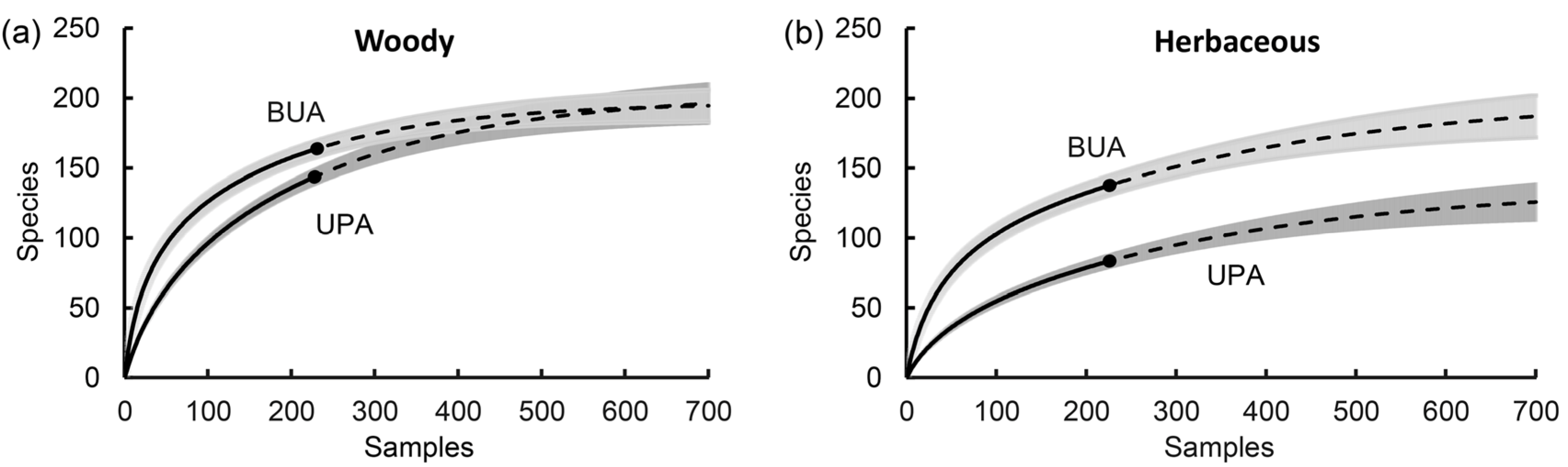
3.1. Species Richness in the Two Areas

We were able to gain access to 229 plots for the UPA and 232 plots for the BUA. Plots where access was denied were mainly on lands occupied by sensitive government agencies. Based on the field records, surveyed sample plots were classified as seven land use types (Figure 2): agricultural areas (AGR); commercial, institutional, or industrial lands (CII); public green spaces (PGS); residential areas (RES); transportation areas (TRA); transitional areas (TRS); and woodlands (WOO). The classification system for assigning the type of land use to each plot is included in Table 1.
Figure 2. The distribution of sample plots in different land use types in the built-up area (BUA) and the urban planning area (UPA). Land use: agricultural areas (AGR); commercial, institutional, or industrial lands (CII); public green spaces (PGS); residential areas (RES); transportation areas (TRA); transitional areas (TRS), and woodlands (WOO).
Forests 07 00042 g002
Table 1. Land use classification system used in this study.
Land UseDescription
Agricultural landAll lands used primarily for the production of food and fiber and associated structures
Commercial, institutional or industrial landsAreas that contain structures predominantly used for sale of products and services and areas occupied by light or heavy industry
Public green spacesGreen spaces that are maintained by a government agency, such as parks and golf courses
Residential areasDensely populated urban zones containing single or multiple dwelling units
Transportation areasAreas that contain transportation routes and facilities
Transitional areasLands for which future land use has not been realized, e.g., areas that are under construction for unknown use, vacant lands, abandoned agricultural land
WoodlandsAreas predominately covered by woody vegetation
A total of 228 species belonging to 186 genera and 71 families were recorded in the UPA. A total of 303 species belonging to 230 genera and 80 families were found in the BUA (Table 2). The 144 woody plant species found in the UPA were from 116 genera and 50 families; the 84 herbaceous plant species were from 72 genera and 32 families. In the BUA, the 164 woody plant species were from 124 genera and 49 families; the 139 herbaceous plant species were from 109 genera and 43 families.
Table 2. Plant species richness of different land uses in the built-up area (BUA) and the urban planning area (UPA).
Land Use aAll PlantsWoodyHerbaceous
UPABUACombinedUPABUACombinedUPABUACombined
AGR580582102137037
CII291952012210811278789
PGS3615416227919896364
RES7519922253117131228291
TRA59104122405469195053
TRS7873121452155335266
WOO10301037207231031
All land uses22830339314416422484139169
Land use: agricultural areas (AGR); commercial, institutional, or industrial lands (CII); public green spaces (PGS); residential areas (RES); transportation areas (TRA); transitional areas (TRS), and woodlands (WOO).
Plant species richness of the different land uses is listed in Table 1. In the BUA, no sample plots were distributed in agricultural areas and woodlands so we recorded zeros for their species richness. Results of Welch t-tests showed that the species richness for the same type of land use obtained from the two surveys was significantly different except for woody plants in PGS and TRS (Table 3).
The rarefaction and extrapolation curves showed estimated plant species richness in the UPA and the BUA by extrapolating the number of sampling plots to 700 (Figure 3). The sample-based rarefaction curves of the UPA and the BUA for woody plant species overlapped at a sample size of 400, which indicated that the difference in total species richness became statistically insignificant above that sample size. However, the curves did not overlap even at three times the sample size for herbaceous plants. This implied that the difference between the species richness of herbaceous plants in the two areas was significant at the 95% confidence interval at that sample size.
Table 3. Welch two sample t-tests on species richness between the built-up area (BUA) and the urban planning area (UPA) grouped by all plant species, native status, vegetation types, and land uses.
CategoriesAll PlantsWoody PlantsHerbaceous Plants
Entire study areap < 0.001p < 0.001p < 0.001
Origin
Native speciesp < 0.001p < 0.001p < 0.001
Exotic speciesp < 0.001p < 0.001p < 0.001
Land use a
CIIp < 0.001p < 0.001p < 0.001
PGSp = 0.020p = 0.122p = 0.004
RESp < 0.001p < 0.001p < 0.001
TRAp = 0.001p = 0.049p = 0.008
TRSp = 0.001p = 0.962p < 0.001
Land use: agricultural areas (AGR); commercial, institutional, or industrial lands (CII); public green spaces (PGS); residential areas (RES); transportation areas (TRA); transitional areas (TRS), and woodlands (WOO).
Figure 3. Sample-based rarefaction and extrapolation for reference samples for (a) woody plant species and (b) herbaceous plant species from the built-up area (BUA) and the urban planning area (UPA) under the Bernoulli product model, with 95% unconditional confidence intervals.
Forests 07 00042 g003
The estimated values of S ˜ sample ( t ) , S ˜ sample ( T + t * ) , t ˜ , ℊ, and the unconditional standard error values (SE) for the interpolated and extrapolated estimates are listed in Table 4. The SE values were relatively small up to a doubling of the reference sample, indicating accurate extrapolation in this range. The species richness of woody plants was greater in the BUA than the UPA for sample sizes up to at least 400 plots. For herbaceous plants, the difference existed up to at least 700 plots.
Table 4. Sample-based interpolation, extrapolation and prediction of number of additional sampling units required to reach S ˜ sample ( T + t * ) and ℊ, under the Bernoulli product model, for woody and herbaceous plants in plots from the built-up area (BUA) and the urban planning area (UPA).
RarefactionExtrapolationSampling Units Prediction
t S ˜ sample ( t ) SEt* S ˜ sample ( T + t * ) SE t ˜
(a) BUA-Woody, Sobs = 164, T = 232
15.370.600164.005.230.8632.15
5095.734.88100178.146.240.9092.36
100126.204.99200186.207.770.94184.09
150144.564.99300190.799.280.98383.90
200157.515.08400193.4110.49
232164.005.23468194.5111.12
(b) UPA-Woody, Sobs = 144, T = 229
12.190.260144.006.500.86170.73
5063.584.12100165.177.990.90248.46
10096.385.08200178.8410.030.94367.18
150118.965.66300187.6712.190.98628.43
200135.906.17400193.3614.13
229144.006.50471196.1315.31
(c) BUA-Herbaceous, Sobs = 139, T = 232
13.520.460139.006.550.86249.74
5075.434.92100155.957.780.90356.27
100102.985.61200168.269.570.94519.00
150119.865.94300177.2011.650.98877.46
200132.316.28400183.7013.75
232139.006.55468187.0715.11
(d) UPA-Herbaceous, Sobs = 84, T = 229
11.380.27084.005.700.86313.05
5036.23.3810098.867.080.90417.00
10054.864.26200109.578.870.94576.07
15068.124.83300117.2810.870.98928.85
20078.695.37400122.8212.85
22984.005.70471125.7914.16

3.2. Difference in Species Composition

The two areas had 138 plant species in common; 35.1% of the total number of species occurred in both areas. They shared 84 woody species, accounting for 37.5% of all woody species found in the two areas. A total of 60 woody species were found in the UPA but not in the BUA. A total of 80 woody plant species were found only in the BUA. There were fewer common herbaceous plants, a total of 54, and only 32% of all herbaceous plant species was recorded in the two areas. A total of 30 and 85 herbaceous species were only recorded in the UPA and the BUA, respectively.
The ten woody plant species that were observed most frequently in sample plots in the two areas are shown in Table 5. For a list of all recorded plant species and their frequencies, please see Table S1 in Supporting Information.
Table 5. Top ten most frequently occurring woody plant species recorded in the built-up area (BUA) and the urban planning area (UPA).
AreaSpeciesOrigin aLife FormFreq.
UPAMelia azedarach L.NTree30
Casuarina equisetifolia L.ETree27
Pterocarpus indicus Willd.ETree21
Lantana camara L.EShrub19
Ficus hispida L.f.NShrub18
Cocos nucifera L.NTree18
Eucalyptus robusta Sm.ETree13
Carica papaya L.ETree12
Pandanus tectorius Parkinson ex Du RoiNShrub12
Psidium guajava L.ETree11
BUAPterocarpus indicus Willd.ETree78
Ficus microcarpa “GoldenLeaves”EShrub68
Ixora chinensis Lam.EShrub66
Cocos nucifera L.NTree52
Hibiscus rosa-sinensis L.EShrub44
Ficus benjamina L.NTree39
Ficus microcarpa L.f.NTree36
Duranta repens “Variegata”EShrub34
Plumeria rubra “Acutifolia”ETree33
Roystonea regia (Kunth) O.F.CookETree32
a. N is for native, E is for exotic. Freq. is for frequency
A total of 39.6% species in the BUA were native and the remaining 60.4% were exotic. The UPA had a lower percentage of exotic species with 49.6% native and 50.4% exotic species.
The βsim index between the two areas for all respective plant species, woody plants, and herbaceous plants was 0.395, 0.417, and 0.357. The βsim of the plant assemblages in different land uses ranged between 0.111 and 0.589 (Table 6). Because no plots were located in agricultural areas and woodlands in the BUA, we did not calculate βsim for these two types of land uses.
Table 6. Floristic dissimilarity (βsim) between the built-up area (BUA) and the urban planning area (UPA) grouped by all plant species, native status, vegetation types, and land uses.
CategoriesAll PlantsWoody PlantsHerbaceous Plants
Entire study area0.3950.4170.357
Origin
Native species0.5400.4640.463
Exotic species0.2520.2290.289
Land use a
  CII0.2070.1820.286
  PGS0.2220.2590.111
  RES0.3070.2640.409
  TRA0.3050.3750.158
  TRS0.5890.4760.424
a Land use: agricultural areas (AGR); commercial, institutional, or industrial lands (CII); public green spaces (PGS); residential areas (RES); transportation areas (TRA); transitional areas (TRS), and woodlands (WOO).

4. Discussion

4.1. Influences of the Delimitations of Study Areas on Quantifying Species Richness

The influences of the delimitations of urban areas on estimates of species diversity of an urban forest were evident from our case study in Haikou. Species richness, a widely used α diversity index, was affected the most. The total plant species richness in the UPA was 25% less than that of the BUA even though the former was four times larger than the latter and the BUA was included in the UPA. The difference is statistically significant as shown by the results of rarefaction analysis. Although this finding seems counterintuitive it was not unexpected.
Larger areas do not necessarily have higher species richness than smaller areas because the species-area curve relationship can be affected both by the ecological process and the sampling effect [32]. In this study, we used the same number of sample plots in both the UPA and BUA. Because the BUA had a higher percentage of commercial and residential land uses to total area than the UPA, the probability of locating more plots in these land use types was higher in the BUA under a random sampling scheme. This was verified by the number of plots sampled in different land uses. Residential areas normally contain higher plant species richness than the surrounding environments because of intentional introduction by humans [33,34,35]. This study found that plant species richness was highest under residential land use with the highest plant species richness, 32, in a single plot in a residential area. On the other hand, more plots were sampled from agricultural lands in the UPA. Plant species richness was lowest in agricultural land use areas. This finding was consistent with the general observation that intensive agriculture lowers species diversity [36]. Therefore, due to the sampling of a high proportion of land uses that had low species richness, a lower overall plant species richness was recorded in the UPA even though the total area was four times that of the BUA.
Differences between species richness observed from same types of land use in the two surveys were largely significant except for woody plants in public green spaces and transitional areas. Significant differences were expected because various types of land use were not sampled equally in the two surveys. The lack of significant difference between woody plant species in public green spaces indicated lack of variation in planting design among public green spaces. Numbers of woody species recorded in each plot did not vary significantly. For transitional areas, the lack of significant difference between the species richness of woody plants was due to the low number of woody plant species recorded in each plot. A total of 67.8% of plots from transitional areas in UPA and 53.9% of plots from transitional areas in BUA recorded one or zero woody plant species.
The overall species richness of woody plants in the two areas converged after extrapolating the sample size to about 400 plots, which indicated that a large sample size may help to reduce the boundary effect. This finding is in accordance with the observation of Jim and Chen [37] in Taipei that urbanization might not have affected overall tree species richness substantially. However, the same did not happen with herbaceous plants, which indicated that a larger sample size would be needed if one wants to study the species diversity of understory plants in urban forests. This may be due to the more heterogeneous response of herbaceous plants to urbanization. Hobbs [38] found that the species richness of herbaceous plants was affected more by human disturbances than trees and shrubs. Trentanovi et al. [39] also found that the species richness of understory native plants of urban woodlands was significantly affected by the urbanity of the site.

4.2. Influences of the Delimitations of Study Areas on Comparing Species Compositions

The results showed that only one third of all plant species was recorded both in the BUA and the UPA. More exotic species were found in the BUA than the UPA. A close look showed that 54 of the 80 woody plant species found only in the BUA were introduced species while the 44 of 60 woody plant species found only in the UPA were native species. The BUA could have been more directly affected by the urbanization process while the UPA included a large area less affected by urbanization. The urbanization process facilitates the establishment of exotic species through several mechanisms [40]. It reduces the diversity of native species by destroying and fragmenting large areas of habitat [41]. Secondly, exotic species are more likely to adapt to a variety of habitats in the city [42,43]. Finally, intentional introduction by humans also contributes to the high percentage of exotic species in urban areas [34].
Frequency of species was used as an indicator to study the composition of urban forests [11,44,45,46]. Studies often report the most frequently occurring woody plant species. This study showed that the two sets of species frequency data would give dramatically different impressions of the urban forests in Haikou City. The lists of the ten most frequently occurring woody plant species in the two studied areas had only two species in common. The two most frequently occurring tree species recorded only in the UPA were M. azedarach, a widely distributed native species in natural areas, and C. equisetifolia, the main species used for constructing coastal greenbelts to protect coastlines from wind and sand erosion. The list of the ten most frequently occurring woody plant species recorded in the UPA showed an urban forest with few synurbic species, a group that has higher population densities in urban areas than rural areas [47]. The list of the ten most frequently occurring woody plant species in the BUA showed an urban forest dominated by synurbic species. All are species widely used in landscaping and gardening.
The βsim index between the two areas for all plant species was 0.395. If all species in the two areas could be recorded, the floristic dissimilarity should be zero because the BUA is a subset of the UPA [31]. The values of βsim showed that native plants in the two areas were more dissimilar than exotic plants, indicating that native species contributed more to the dissimilarity of plant communities than exotic species. The UPA could also contain more native species due to the existence of large areas impacted less strongly by the urbanization process.
The highest floristic dissimilarity of different land use types between the two areas occurred in transitional areas. The high floristic dissimilarity between transitional areas in the UPA and the BUA reflected two different ecological processes. Transitional areas in the BUA consisted primarily of undeveloped or demolished building sites. Soil compaction, pollutants, and other urban environmental stresses in these sites favor stress-tolerant and ruderal species [10,47,48]. The most frequently occurring herbaceous species found on these lands (e.g., Eleusine. indica (L.) Gaertn, Melinis repens (Wild.) Zizka, and Sesbania cannabina (Retz.) Pers.) were all ruderal species. Spontaneous woody vegetation was rare and did not form large patches in BUA as found in other studies [49,50]. This may be due to the fast turnover of lands inside the built-up areas in Chinese cities [51]. Transitional areas in the UPA were mainly fallowed agricultural lands distributed among agricultural lands and villages. These sites provided good habitats for many native species because they were relieved from the pressure of intensive management in agricultural lands [52]. A total of 48 out of 78 species found in these sites were native species.

4.3. Implications for Urban Forestry Studies

The results of our study showed that the influence of the different delimitations of urban areas was obvious with respect to the assessment of species diversities of urban forests in general and more so with respect to the biodiversity indexes based on species richness. The overall species richness differed by as much as 25% in two nested areas sampled using the same sampling scheme. The floristic dissimilarity was also evident even though the Simpson dissimilarity index was used. This observation confirmed the need for clarifying the effects of sampling effort on richness measures and comparisons [53]. Comparison studies and meta-analysis that use pooled species diversity data of urban forests should be conducted but only if special attention is paid to how urban areas were defined in the different studies. Boundaries of study areas in ecological studies carried out in natural environments can often be identified by obvious physical discontinuities in nature [54], but the boundaries of urban areas are frequently defined by arbitrary political and social-economic factors. In order to facilitate more comparative studies, we suggest that researchers should adopt a standard sampling procedure such as the one specified in the i-Tree Eco User's Manual [55] and define the spatial boundaries of study areas clearly in future studies. A possible way to lower the influence of the different delimitations of urban areas is to use stratified sampling. Proportional stratified sampling can allocate sample plots based on percentage urban forest canopy cover of different types of land use, thus allowing for better representation of the whole urban forest.
Our results also have implications for urban biodiversity conservation. It is important for planners and policy-makers to clearly identify the boundaries of urban areas. Since socio-economic changes can cause urban boundaries to expand or shrink, caution must be taken when assessing the effectiveness of conservation efforts because comparisons made on areas that are not equal could result in misleading conclusions.
It should be noted that this study verified the influence of two different delimitations of urban areas on estimates of species diversity of an urban forest in China. Cities often go through different urbanization processes so the impacts of urbanization on species diversity of urban forests could vary in other cities. More studies are needed to determine the impact on cities that go through different development pathways. Furthermore, the current study only focused on the impact on assessing the taxonomic diversity of an urban forest and did not study the influence on the functional diversity. Plant functional groups respond differently to impacts of urbanization and conservation strategies need to focus on functional groups with high conservational value [56]. Therefore, the impact of different delimitations of urban areas on assessing the functional diversity of an urban forest need to be addressed in future studies as well.

5. Conclusions

The delimitation of the study area is one of the many factors affecting our assessments of species diversities of urban forests. In this study, we examined the impacts of using two different delimitations of urban areas on the survey results of species diversity of an urban forest. Our results showed that the different delimitations led to significantly different estimates of species richness of a same urban forest. The inclusion of different proportions of various land use types in samples when using different delimitations of urban areas contributed to this difference. To our knowledge, our study was the first one that used real data to prove the long-suspected influence of the delimitation of study area on studying plant species in urban environments. While more studies are needed to verify the effect in cities with different socio-economic backgrounds, we suggest that caution should be taken when comparing species diversities of urban forests reported in different studies.

Supplementary Materials

The following are available online at www.mdpi.com/1999-4907/7/2/42/s1.

Acknowledgments

We thank Mingxun Ren, Zhenzhen Pang, and Qiong Ding for their helpful comments. We also thank the graduate students at the College of Horticulture and Landscape Architecture, Hainan University for their help in collecting field data. This research was supported by grants from the National Natural Science Foundation of China (No. 31160178, No. 31570458), Hainan University Postgraduate Outstanding Thesis Development Program, and the Academic discipline construction project plan in the central and western regions of Hainan University (ZXBJH-XK008).

Author Contributions

Jun Yang designed the study. Rongxiao He led the field survey. Jun Yang, Rongxiao He, and Xiqiang Song all contributed to the writing of the paper.

Conflicts of Interest

The authors declare no conflict of interest.

References

  1. Department of Economic and Social Affairs. World Urbanization Prospects: The 2014 Revision, Highlights (ST/ESA/SER.A/352); the United Nations: New York, NY, USA, 2014. [Google Scholar]
  2. Seto, K.C.; Güneralp, B.; Hutyra, L.R. Global forecasts of urban expansion to 2030 and direct impacts on biodiversity and carbon pools. Proc. Nat. Acad. Sci. USA 2012, 109, 16083–16088. [Google Scholar] [CrossRef] [PubMed]
  3. Dearborn, D.C.; Kark, S. Motivations for conserving urban biodiversity. Conserv. Biol. 2010, 24, 432–440. [Google Scholar] [CrossRef] [PubMed]
  4. Alvey, A.A. Promoting and preserving biodiversity in the urban forest. Urban For. Urban Green. 2006, 5, 195–201. [Google Scholar] [CrossRef]
  5. Goddard, M.A.; Dougill, A.J.; Benton, T.G. Scaling up from gardens: Biodiversity conservation in urban environments. Trends Ecol. Evol. 2010, 25, 90–98. [Google Scholar] [CrossRef] [PubMed]
  6. Miller, R.W. Urban Forestry: Planning and Managing Urban Greenspaces; Prentice Hall: Upper Saddle River, NJ, USA, 1988. [Google Scholar]
  7. Sanders, R.A.; Stevens, J.C. Urban forest of Dayton, Ohio: A preliminary assessment. Urban Ecol. 1984, 8, 91–98. [Google Scholar] [CrossRef]
  8. Pauleit, S.; Jones, N.; Garcia-Martin, G.; Garcia-Valdecantos, J.L.; Rivière, L.M.; Vidal-Beaudet, L.; Bodson, M.; Randrup, T.B. Tree establishment practice in towns and cities—Results from a European survey. Urban For. Urban Green. 2002, 1, 83–96. [Google Scholar] [CrossRef]
  9. Nowak, D.J. Urban biodiversity and climate change. In Urban Biodiversity and Design; Müller, N., Werner, P., Kelcy, J.G., Eds.; Wiley-Blacwell: Hoboken, NJ, USA, 2010; Volume 5, pp. 101–117. [Google Scholar]
  10. Nowak, D.J. Contrasting natural regeneration and tree planting in fourteen North American cities. Urban For. Urban Green. 2012, 11, 374–382. [Google Scholar] [CrossRef]
  11. Yang, J.; McBride, J.; Zhou, J.; Sun, Z. The urban forest in Beijing and its role in air pollution reduction. Urban For. Urban Green. 2005, 3, 65–78. [Google Scholar] [CrossRef]
  12. Kendal, D.; Williams, N.S.; Williams, K.J. A cultivated environment: Exploring the global distribution of plants in gardens, parks and streetscapes. Urban Ecosyst. 2012, 15, 637–652. [Google Scholar] [CrossRef]
  13. McKinney, M.L. Effects of urbanization on species richness: A review of plants and animals. Urban Ecosyst. 2008, 11, 161–176. [Google Scholar] [CrossRef]
  14. Pyšek, P. Factors affecting the diversity of flora and vegetation in central European settlements. Vegetatio 1993, 106, 89–100. [Google Scholar] [CrossRef]
  15. Nowak, D.J.; Walton, J.T.; Stevens, J.C.; Crane, D.E.; Hoehn, R.E. Effect of plot and sample size on timing and precision of urban forest assessments. Arboric. Urban For. 2008, 34, 386–390. [Google Scholar]
  16. Alvarez, I.A.; del Nero Velasco, G.; Barbin, H.S.; Lima, A.; do Couto, H.T.Z. Comparison of two sampling methods for estimating urban tree density. J. Arboric. 2005, 31, 209. [Google Scholar]
  17. Tait, C.J.; Daniels, C.B.; Hill, R.S. Changes in species assemblages within the Adelaide Metropolitan Area, Australia, 1836–2002. Ecol. Appl. 2005, 15, 346–359. [Google Scholar] [CrossRef]
  18. McIntyre, N.E.; Knowles-Yánez, K.; Hope, D. Urban ecology as an interdisciplinary field: Differences in the use of “urban” between the social and natural sciences. Urban Ecosyst. 2000, 4, 5–24. [Google Scholar] [CrossRef]
  19. Wu, J. Urban ecology and sustainability: The state-of-the-science and future directions. Landsc. Urban Plan. 2014, 125, 209–221. [Google Scholar] [CrossRef]
  20. Hainan Bureau of Statistics. Hainan Statistics Yearbook 2014; China Statistics Press: Beijing, China, 2014.
  21. Xing, F.; Zhou, J.; Wang, F.; Zeng, Q.; Yi, Q.; Liu, D. Inventory of Plant Species Diversity of Hainan; Huazhong University of Science & Technology Press: Wuhan, China, 2012. [Google Scholar]
  22. Kendal, D.; Williams, N.S.G.; Williams, K.J.H. Drivers of diversity and tree cover in gardens, parks and streetscapes in an Australian city. Urban For. Urban Green. 2012, 11, 257–265. [Google Scholar] [CrossRef]
  23. Milović, M.; Mitić, B. The urban flora of the city of Zadar (Dalmatia, Croatia). Nat. Croat. 2012, 21, 65–100. [Google Scholar]
  24. Wang, G.; Zuo, J.; Li, X.; Liu, Y.; Yu, J.; Shao, H.; Li, Y. Low plant diversity and floristic homogenization in fast-urbanizing towns in Shandong Peninsular, China: Effects of urban greening at regional scale for ecological engineering. Ecol. Eng. 2014, 64, 179–185. [Google Scholar] [CrossRef]
  25. Zhao, J.; Ouyang, Z.; Zheng, H.; Zhou, W.; Wang, X.; Xu, W.; Ni, Y. Plant species composition in green spaces within the built-up areas of Beijing, China. Plant. Ecol. 2010, 209, 189–204. [Google Scholar] [CrossRef]
  26. Guangdong Institute of Botany. Flora of Hainan; Science Press: Beijing, China, 1974. [Google Scholar]
  27. South China Botanical Garden. Flora of Guangdong; Guangdong Science and Technology Press: Guangzhou, China, 2009. [Google Scholar]
  28. Ricotta, C.; Pavoine, S.; Bacaro, G.; Acosta, A.T. Functional rarefaction for species abundance data. Methods Ecol. Evol. 2012, 3, 519–525. [Google Scholar] [CrossRef]
  29. Colwell, R.K.; Chao, A.; Gotelli, N.J.; Lin, S.Y.; Mao, C.X.; Chazdon, R.L.; Longino, J.T. Models and estimators linking individual-based and sample-based rarefaction, extrapolation and comparison of assemblages. J. Plant. Ecol. 2012, 5, 3–21. [Google Scholar] [CrossRef]
  30. EstimateS, version 9.1.0. Robert K. Colwell: Storrs, CT, USA, 2014. Available online: http://purl.oclc.org/estimates (accessed on 11 May 2015).
  31. Baselga, A. Partitioning the turnover and nestedness components of beta diversity. Glob. Ecol. Biogeogr. 2010, 19, 134–143. [Google Scholar] [CrossRef]
  32. Hill, J.L.; Curran, P.J.; Foody, G.M. The effect of sampling on the species-area curve. Glob. Ecol. Biogeogr. Lett. 1994, 97–106. [Google Scholar] [CrossRef]
  33. Hope, D.; Gries, C.; Zhu, W.; Fagan, W.F.; Redman, C.L.; Grimm, N.B.; Nelson, A.L.; Martin, C.; Kinzig, A. Socioeconomics drive urban plant diversity. Proc. Nat. Acad. Sci. USA 2003, 100, 8788–8792. [Google Scholar] [CrossRef] [PubMed]
  34. Kowarik, I.; Lippe, M.; Cierjacks, A. Prevalence of alien versus native species of woody plants in Berlin differs between habitats and at different scales. Preslia 2013, 85, 113–132. [Google Scholar]
  35. Walker, J.S.; Grimm, N.B.; Briggs, J.M.; Gries, C.; Dugan, L. Effects of urbanization on plant species diversity in central Arizona. Front. Ecol. Environ. 2009, 7, 465–470. [Google Scholar] [CrossRef]
  36. Karp, D.S.; Rominger, A.J.; Zook, J.; Ranganathan, J.; Ehrlich, P.R.; Daily, G.C. Intensive agriculture erodes β-diversity at large scales. Ecol. Lett. 2012, 15, 963–970. [Google Scholar] [CrossRef] [PubMed]
  37. Jim, C.Y.; Chen, W.Y. Pattern and divergence of tree communities in Taipei’s main urban green spaces. Landsc. Urban Plan. 2008, 84, 312–323. [Google Scholar] [CrossRef]
  38. Hobbs, E.R. Species richness of urban forest patches and implications for urban landscape diversity. Landsc. Ecol. 1988, 1, 141–152. [Google Scholar] [CrossRef]
  39. Trentanovi, G.; Lippe, M.; Sitzia, T.; Ziechmann, U.; Kowarik, I.; Cierjacks, A. Biotic homogenization at the community scale: Disentangling the roles of urbanization and plant invasion. Divers. Distrib. 2013, 19, 738–748. [Google Scholar] [CrossRef]
  40. Williams, N.S.G.; Schwartz, M.W.; Vesk, P.A.; McCarthy, M.A.; Hahs, A.K.; Clemants, S.E.; Corlett, R.T.; Duncan, R.P.; Norton, B.A.; Thompson, K.; et al. A conceptual framework for predicting the effects of urban environments on floras. J. Ecol. 2009, 97, 4–9. [Google Scholar] [CrossRef]
  41. Doody, B.J.; Sullivan, J.J.; Meurk, C.D.; Stewart, G.H.; Perkins, H.C. Urban realities: The contribution of residential gardens to the conservation of urban forest remnants. Biodivers. Conserv. 2010, 19, 1385–1400. [Google Scholar] [CrossRef]
  42. Deutschewitz, K.; Lausch, A.; Kühn, I.; Klotz, S. Native and alien plant species richness in relation to spatial heterogeneity on a regional scale in Germany. Global Ecol. Biogeogr. 2003, 12, 299–311. [Google Scholar] [CrossRef]
  43. Ricotta, C.; Godefroid, S.; Rocchini, D. Patterns of native and exotic species richness in the urban flora of Brussels: Rejecting the “rich get richer” model. Biol. Invasions 2010, 12, 233–240. [Google Scholar] [CrossRef]
  44. Bourne, K.S.; Conway, T.M. The influence of land use type and municipal context on urban tree species diversity. Urban Ecosyst. 2013, 17, 329–348. [Google Scholar] [CrossRef]
  45. Lamichhane, D.; Thapa, H.B. Participatory urban forestry in Nepal: Gaps and ways forward. Urban For. Urban Green. 2012, 11, 105–111. [Google Scholar] [CrossRef]
  46. Yang, J.; Zhou, J.; Ke, Y.; Xiao, J. Assessing the structure and stability of street trees in Lhasa, China. Urban For. Urban Green. 2012, 11, 432–438. [Google Scholar] [CrossRef]
  47. Francis, R.A.; Chadwick, M.A. What makes a species synurbic? Appl. Geogr. 2012, 32, 514–521. [Google Scholar] [CrossRef]
  48. Duncan, R.P.; Clemants, S.E.; Corlett, R.T.; Hahs, A.K.; McCarthy, M.A.; McDonnell, M.J.; Schwartz, M.W.; Thompson, K.; Vesk, P.A.; Williams, N.S.G. Plant traits and extinction in urban areas: A meta-analysis of 11 cities. Global Ecol. Biogeogr. 2011, 20, 509–519. [Google Scholar] [CrossRef]
  49. Kunick, W. Woody vegetation in settlements. Landscape Urban Plan. 1987, 14, 57–78. [Google Scholar] [CrossRef]
  50. Sitzia, T.; Campagnaro, T.; Weir, R.G. Novel woodland patches in a small historical Mediterranean city: Padova, northern Italy. Urban Ecosyst. 2015. [Google Scholar] [CrossRef]
  51. Yang, J.; Huang, C.; Zhang, Z.; Wang, L. The temporal trend of urban green coverage in major Chinese cities between 1990 and 2010. Urban For. Urban Green. 2014, 13, 19–27. [Google Scholar] [CrossRef]
  52. Firbank, L.G.; Petit, S.; Smart, S.; Blain, A.; Fuller, R.J. Assessing the impacts of agricultural intensification on biodiversity: A British perspective. Phil. Trans. Roy. Soc. B Biol. Sci. 2008, 363, 777–787. [Google Scholar] [CrossRef] [PubMed]
  53. Gotelli, N.J.; Colwell, R.K. Quantifying biodiversity: Procedures and pitfalls in the measurement and comparison of species richness. Ecol. Lett. 2001, 4, 379–391. [Google Scholar] [CrossRef]
  54. Strayer, D.L.; Power, M.E.; Fagan, W.F.; Pickett, S.T.; Belnap, J. A classification of ecological boundaries. BioScience 2003, 53, 723–729. [Google Scholar] [CrossRef]
  55. USDA Forest Service. i-Tree Eco User’s Manual. Available online: http://www.itreetools.org/resources/manuals/i-Tree%20Eco%20Users%20Manual.pdf (accessed on 31 January 2015).
  56. Godefroid, S.; Koedam, N. How important are large vs. small forest remnants for the conservation of the woodland flora in an urban context? Global Ecol. Biogeogr. 2003, 12, 287–298. [Google Scholar] [CrossRef]

