Land Use and Landscape Pattern Changes in the Sanjiang Plain, Northeast China

Abstract

Agricultural reclamation has been the major threat to land use changes in the Sanjiang Plain, Northeast China, over the past decades. However, spatial and temporal dynamics of land use and landscape, especially in the recent years, are not well known. In this study, land use and landscape pattern changes from 1982 to 2015 were analyzed using remote sensing data by splitting the period into five periods. The results indicated that the largest reduction of forestland area was 648.70 km² during 1995–2000, and the relative change was −1.84%. The converted area of forestlands to dry farmlands in this period was about 90% of the total reduced forestland area. Marshland areas decreased remarkably by 63.29% and paddy fields increased by 1.78 times from 1982 to 2015. Paddy fields experienced large conversion into dry farmlands during 2005–2010 (1788.57 km²), followed by a reverse conversion from 1995 to 2000 (2379.60 km²). The difference of relative change revealed development speed of paddy field was faster than that of dry farmlands among the five periods. Landscape pattern was analyzed using class- and landscape-level metrics. The landscape diversity index and number of patches increased, which showed that the degrees of the forestland, marshland, and cropland landscape fragmentation were aggravated. Our study provides the effective means of land use dynamic monitoring and evaluation at the landscape level for the existing forestlands and marshlands protection.

1. Introduction

Forests, wetlands, and oceans are known as the three major ecosystems in the Earth. Wetlands are the important components of the terrestrial ecosystems, providing significant ecosystem services as climate regulation, flood storage, water supply, and biodiversity conservation [1]. Climate change leads to increases in the frequency and magnitude of floods and droughts [2], augmenting the vulnerability of wetland ecosystems. Nearly half of the world’s wetlands have been lost by hydrological alterations associated with agricultural reclamation [3]. Recent policy frameworks are being well developed, but wetland degradation is still widespread [4].

Recently, wetlands worldwide have the fastest loss rates among any ecosystems [5]. However, precisely complete wetland loss data cannot be available because of the different definitions and techniques employed by the various assessments. In a generalized perspective, 50% of wetlands in the Earth may have been lost since 1900, mainly due to agricultural extension [6]. The increase of population has put wetlands at risk [7]. Wetlands have been extensively drained for economic development. Direct wetland conversion for agricultural drainage, forestry, as well as urban construction, has caused wetland destruction and degradation [8,9]. Thus, further research is needed to produce more sustainable socio-ecosystems [10]. Restoration actions that enhance both biodiversity and other ecosystem services are necessary worldwide [11,12,13]. In this study, we chose the Sanjiang Plain, Northeast China, as a study site, which possesses large areas of marshlands and is characterized as the important food base of China. The area of croplands in the Naoli River catchment accounts for one-third of the total croplands in the Sanjiang Plain.

Land use types have different change processes, such as forestlands and grasslands in Northeast China, which were converted chiefly to farmlands [14,15]. However, the important characteristics of land use changes among forestlands, paddy fields, dry farmlands remain uncertain, especially the spatial pattern changes. Many studies have investigated marshlands loss and landscape changes in the Sanjiang Plain [16,17,18,19]. Remote sensing and GIS technologies are usually applied for the landscape pattern changes. It is paid less attention to the comparison of forestlands or marshlands conversion into croplands in different time periods. The contradictions are concentrated among marshlands, paddy fields, and dry farmlands. The landscape pattern indices mainly focus on spatial characteristics of the landscape or land use types. We used over 30-year images to analyze land use and landscape pattern changes. How land use changes in recent years or whether the changes are still continuing remains uncertain. The spatial and temporal dynamics of land use, especially in the recent years, need to be further clarified.

In this study, the land use changes in 1982, 1995, 2000, 2005, 2010, and 2015 based on remote sensing data were revealed. The landscape pattern changes in different years on class- and landscape-level metrics by landscape pattern indices were analyzed. It could be a valuable reference for guiding the degraded marshland restoration on the spatial scale.

2. Materials and Methods

2.1. Study Area

Our study area, the Naoli River catchment (45°43′–47°45′ N, 131°31′–134°10′ E) covers 24.20 × 10³ km² within the Sanjiang Plain, Northeast China. The river’s overall length is 283 km. The catchment lies in a temperate zone with the continental monsoon climate. The mean annual temperature is 1.6 °C, with an average temperature of −21.6 °C in January and 21.4 °C in July. The mean annual precipitation is 565 mm, while the mean annual actual evaporation is 542.4 mm. The terrain in the Naoli River catchment is flat and low, with an average altitude of about 60 m. The “Agricultural Modernization” policy by the Chinese government has led to reclaim marshlands in the Sanjiang Plain since 1978 [19,20]. Agricultural development for food has been the main cause of marshlands reclaimed in this region.

2.2. Land Use and Data Sources

We included nine land use types, including forestland, grassland, river and lake, reservoir and pond, marshland, paddy field, dry farmland, salinity and bare land, and residence and construction. In view of agricultural activities, especially cropland reclamation, there are four land use types, which have been thoroughly studied including forestland, marshland, paddy field, and dry farmland. Land use data of 1982 was obtained from the Institute of Remote Sensing and Geographic Information Research Center, Northeast Institute of Geography and Agricultural Ecology (http://marsh.neigae.csdb.cn/). Land use data of 1995, 2000, 2005, 2010, and 2015 were obtained from 10 images of Landsat Thematic Mapper (TM) remote sensing data with a resolution of 30 m. These Landsat TM images were downloaded (http://glovis.usgs.gov/) and digitized by visual interpretation technology. ArcGIS10.2.1 (Esri, Redlands, CA, USA) was used to classify land use types and to generate land use thematic maps. Remote sensing images recorded from June to October were selected because land use types are easy to identify during this period, when plants grow actively in Northeast China. The final land use maps were successfully extracted with the detailed spatial distributions of land use types and their areas. We used these data to investigate the land use and landscape pattern changes.

2.3. Land Use Changes

We calculated the land use conversion areas based on the remote sensing data. We used land use relative change to quantify the land use changes in the time period of 1982–2015, which reflects landscape area can be expanded or shrunk. The land use relative change can be calculated using the following equation:

$$R_S=\frac{U_f-U_i}{U_i}\times \frac{1}{T}\times 100\%$$

(1)

where R_S is land use relative change, U_i and U_f are land use type area at the initial and end-stage of study, respectively, and T is the period of study.

2.4. Landscape Pattern Changes

We used class- and landscape-level metrics to quantify the landscape pattern changes in our study. The indices of landscapes contribute identified numerical information concerning the composition and the patterns of landscapes, the proportion of each land use type, and the spatial heterogeneity of the elements in the landscape. The indices used to characterize landscape patterns from 1982 to 2015 are as follows (see

Table 1. Indices on class- or landscape-level metrics.

Metrics	Indices	Description	Units
Class	LPI	It quantifies the percentage of total landscape area comprised by the largest patch.	Percent
Class	FRAC_AM	It reflects shape complexity across a range of spatial scales.	None
Class	AI	It shows the connectivity of different pairs of patch types.	Percent
Class	SPLIT	It is based on the cumulative patch area distribution and is interpreted as the effective mesh number.	None
Class/landscape	NP	It shows the number of patches.	None
Class/landscape	COHESION	It measures the physical connectedness of the corresponding patch type	None
Landscape	SHAPE_AM	It reflects the complication of landscape pattern.	None
Landscape	CONTAG	It considers all patch types present on an image, including any present in the landscape border.	Percent
Landscape	IJI	It isolates the interspersion or intermixing of patch types.	Percent
Landscape	SHDI	It is used to compare different landscapes or the same landscape at different times.	None
Landscape	SHEI	It is expressed that an even distribution of area among patch type results in the maximum evenness.	None

Number of Patches (NP), Largest Patch index (LPI), Area-Weighted Mean Fractal Dimension index (FRAC_AM), Patch Cohesion index (COHESION), Splitting index (SPLIT), Aggregation index (AI); landscape-level metrics besides NP and COHESION, Area-Weighted Mean Shape index (SHAPE_AM), Contagion (CONTAG), Interspersion and Juxtaposition index (IJI), Shannon’s diversity index (SHDI), Shannon’s Evenness index (SHEI).

): class-level metrics including Number of Patches (NP), Largest Patch index (LPI), Area-Weighted Mean Fractal Dimension index (FRAC_AM), Patch Cohesion index (COHESION), Splitting index (SPLIT), Aggregation index (AI); landscape-level metrics besides NP and COHESION, Area-Weighted Mean Shape index (SHAPE_AM), Contagion (CONTAG), Interspersion and Juxtaposition index (IJI), Shannon’s diversity index (SHDI), and Shannon’s Evenness index (SHEI). They are run in Fragstats v4.2.1 software. Fragstats software supported the format of Geo TIFF grid. We used it to analyze the above indices base on the grid maps of forestland, marshland, paddy field, and dry farmland from 1982 to 2015.

3. Results

3.1. Land Use Changes

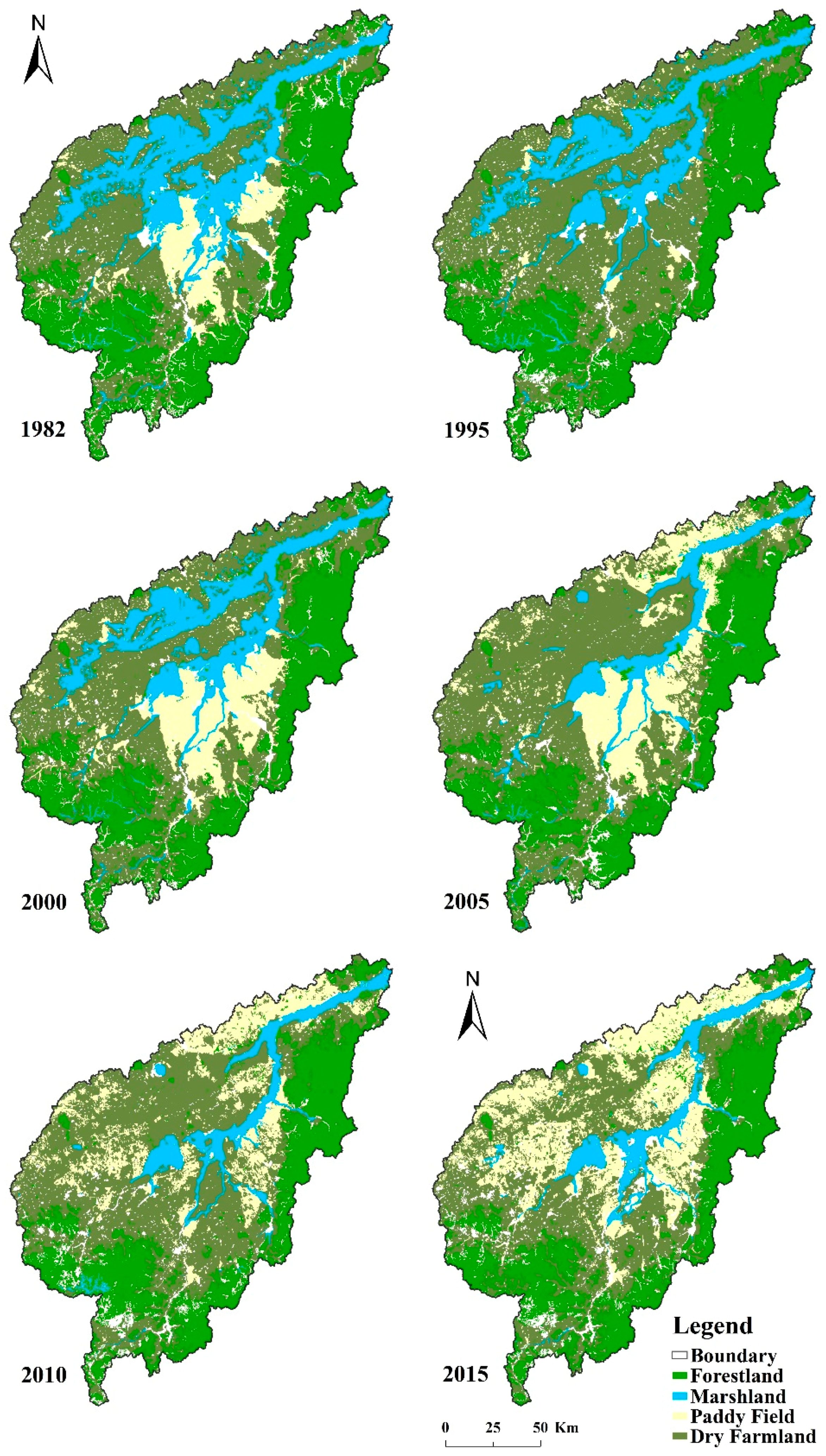
In this study, we analyzed land use and landscape pattern changes based on remote sensing data. The distributions of forestland, marshland, paddy field and dry farmland, and their proportions in 1982, 1995, 2000, 2005, 2010, and 2015 were demonstrated (see Figure 1 and

Table 2. Proportion of land use types from 1982 to 2015 (%).

	1982	1995	2000	2005	2010	2015	Rate of Change
Marshland	18.44	15.64	14.72	7.62	6.83	6.77	−63.29
Paddy Field	8.25	2.00	12.31	16.26	13.91	22.93	177.84
Dry Farmland	37.69	47.53	41.39	45.66	47.38	37.68	−0.01
Forestland	29.95	29.94	27.18	26.44	26.67	26.10	−12.88

). The marshland area was 4336.4 km² in 1982, accounting for 18% of the total study area (see Figure 1).

It was indicated that the marshlands decreased remarkably by 63.29%, forestlands decreased by 12.88%, and dry farmlands decreased by 0.01% from 1982 to 2015. However, paddy fields increased 1.78 times during this period (see Table 2). From 1982 to 2015, the increasing proportion of paddy fields was much higher than that of the decreasing proportion of marshlands.

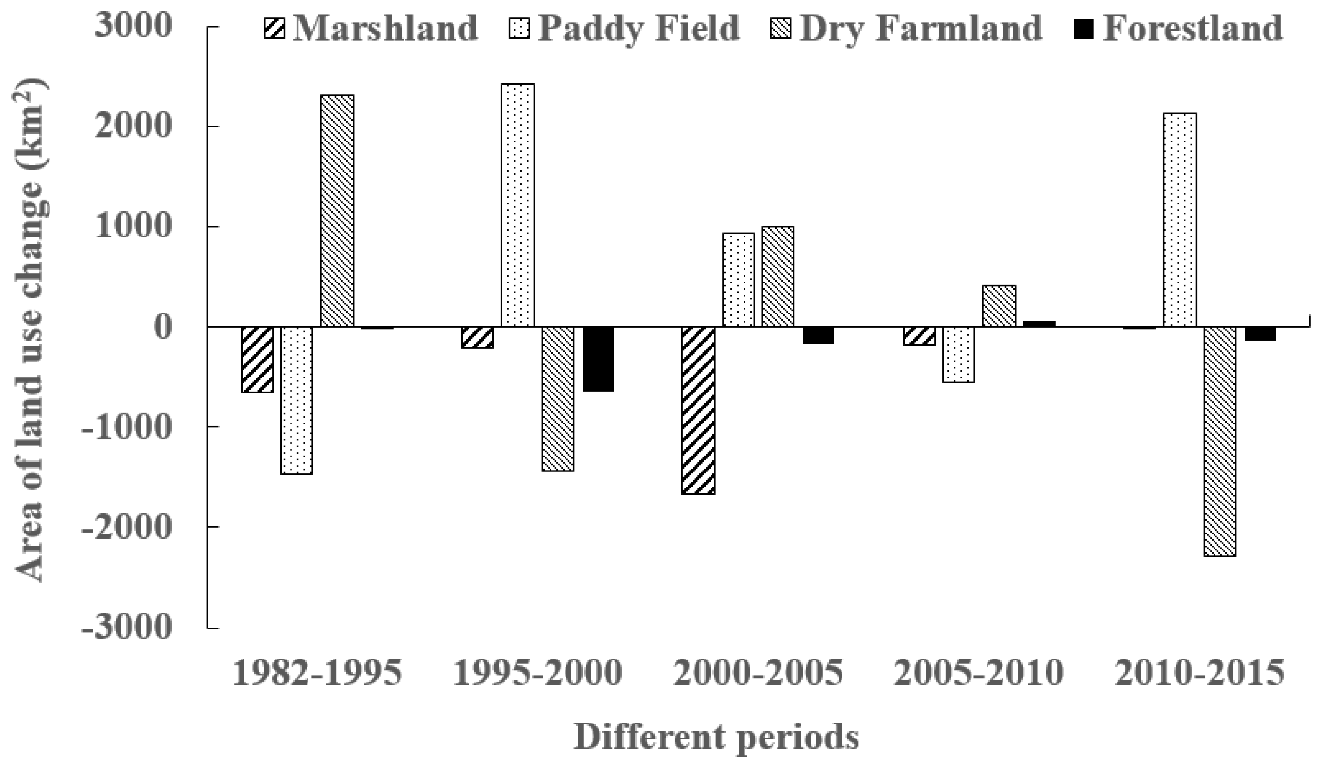
In different periods, the characteristic of mutual conversion between paddy fields and dry farmlands was quite distinguishing. Paddy fields experienced large conversion into dry farmlands during 2005–2010 (1788.57 km²), followed by a reverse conversion from 1995 to 2000 (2379.60 km²) (see

Table 3. Land use conversion and relative change in different periods (km², %).

	Types	1982–1995	1995–2000	2000–2005	2005–2010	2010–2015
Land use conversion	Conversion of paddy field to dry farmland	1737.40	81.11	573.63	1788.57	181.12
	Conversion of dry farmland to paddy field	284.44	2379.60	1298.30	1297.40	2272.20
	Conversion of marshland to paddy field	42.90	46.10	234.10	58.80	76.70
	Conversion of marshland to dry farmland	759.40	227.00	1590.20	276.60	98.60
	Conversion of forestland to dry farmland	290.90	578.70	364.30	386.30	575.20
Land use relative change	Marshland	−1.17	–1.18	–9.64	–2.08	–0.17
	Paddy field	–5.83	103.05	6.41	–2.89	12.97
	Dry farmland	2.01	–2.58	2.07	0.75	–4.09
	Forestland	–0.003	–1.84	–0.54	0.17	–0.43

). Therefore, the biggest amplitude of dry farmlands conversion to paddy fields was between 1995 and 2000 with a relative change of 103.05% (see Table 3). In general, the exploitation scale of paddy fields was enlarged obviously. The total converted quantities of marshlands to dry farmlands were significantly higher than those of marshlands to paddy fields in various stages. The relative change of paddy fields was higher than that of dry farmlands, which indicated that the development speed of paddy field was faster than that of dry farmlands among the five periods. From 1995 to 2000 and 2010 to 2015, the relative change of paddy fields was always positive compared with that of marshlands and dry farmlands, so it was revealed that paddy fields expanded remarkably in these two periods.

There is no obvious difference in the proportions of forestlands from 1982 to 2015, with the maximum proportion of 29.95% in 1982 and the minimum proportion of 26.10% in 2015 (see Table 2). The largest reduction of forestland area was 648.70 km² from 1995 to 2000 and the relative change was −1.84% (see Figure 2 and Table 3). There was 578.70 km² of forestlands conversion to dry farmlands in this period (see Table 3). Therefore, it was about 90% of the largest reduced forestland area from 1995 to 2000.

3.2. Landscape Pattern Changes

Delta (Δ) means difference in our study. As shown in

Table 4. Class-level metrics for marshlands, paddy fields and dry farmlands in the Naoli River catchment.

	Type	NP	LPI	FRAC_AM	COHESION	SPLIT	AI
1982	Marshland	153	9.89	1.20	99.95	102.12	99.36
	Paddy field	120	29.90	1.13	99.83	4.95	99.15
	Dry farmland	382	51.58	1.25	99.95	3.31	98.61
1995	Marshland	124	8.47	1.20	99.94	139.34	99.33
	Paddy field	301	9.02	1.08	98.60	30.94	97.00
	Dry farmland	324	68.09	1.27	99.98	2.07	98.81
2000	Marshland	124	6.50	1.17	99.92	232.02	99.35
	Paddy field	325	23.72	1.14	99.76	6.99	98.80
	Dry farmland	557	59.89	1.27	99.96	2.60	98.47
2005	Marshland	116	3.57	1.16	99.87	781.30	99.20
	Paddy field	383	18.36	1.17	99.80	9.85	98.51
	Dry farmland	258	77.54	1.22	99.98	1.65	99.36
2010	Marshland	49	2.72	1.16	99.88	1267.44	99.28
	Paddy field	725	28.89	1.20	99.73	10.04	97.55
	Dry farmland	689	67.37	1.29	99.97	2.12	98.31
2015	Marshland	59	1.73	1.15	99.85	1909.46	99.27
	Paddy field	870	20.81	1.21	99.82	10.70	98.05
	Dry farmland	1213	58.88	1.29	99.95	2.73	97.58
1982–2015	Marshland	−94	−8.17	−0.06	−0.10	1807.34	−0.09
	Paddy field	750	−9.08	0.08	−0.01	5.74	−1.10
	Dry farmland	831	7.30	0.04	−0.002	−0.58	−1.04

, from 1982 to 2015, ΔLPI, and ΔFRAC_AM of paddy fields were higher than those of marshlands and dry farmlands, which indicated stronger human intervention and severe landscape fragmentation. ΔNP of paddy fields and dry farmlands were obviously higher than that of marshlands, which showed that the intensity of cropland exploitation was increased especially after 1995.

ΔSPLIT of marshlands was 1807.34 from 1982 to 2015, obviously higher than that of paddy fields and dry farmlands, so they were much scattered. On the other hand, ΔAI of marshlands was smallest from 1982 to 2015, and meanwhile, ΔCOHESION of marshlands had the maximum amplitude with the trend of fluctuation, which indicated that patch connectivity was not compact.

Clear evidences of this fragmentation process can be observed on the remaining landscape-level metrics (see

Table 5. Landscape-level metrics for marshlands, paddy fields and dry farmlands in the Naoli River catchment.

	NP	CONTAG	IJI	COHESION	SHDI	SHEI
1982	727	74.24	31.85	99.94	1.03	0.50
1995	768	79.85	25.77	99.96	0.75	0.39
2000	1199	70.41	41.66	99.94	1.11	0.57
2005	1323	67.47	48.69	99.94	0.86	0.62
2010	1485	74.84	20.41	99.95	0.92	0.47
2015	2192	68.54	25.76	99.91	1.16	0.60

). IJI significantly decreased with a more scattered pattern of landscape from 1982 to 2015. Meanwhile, NP rapidly increased, which led to a clear fragmentation process.

CONTAG had obvious difference with a range of 5.69%, and there were dominant patches with high connectivity. Because the range of CONTAG value was from 0 to 100%, the CONTAG in our study was about 70% in the direction of 100%. COHESION was about 99.9 with no particularly obvious change in different years, which showed that landscape connectivity was sustained.

The SHDI value reached the maximum in 2015, and meanwhile, the SHEI value in 2015 was much higher, which meant that the landscape area ratio tended to be further heterogeneous. Hence, there was a more even distribution of the patch types in landscape.

There are four subtypes of forestlands, including thick woodland, shrub land, sparse woodland, and others. As shown in

Table 6. Class-level metrics for forestlands in the Naoli River catchment.

	Subtype	NP	LPI	FRAC_AM	COHESION	SPLIT	AI
1982	Thick woodland	173	43.98	1.20	99.96	2.93	99.33
	Shrub land	112	0.55	1.06	98.71	15,342.53	97.86
	Sparse woodland	39	0.45	1.06	98.70	45,558.20	98.02
	Others	17	0.05	1.03	97.49	151,3231.96	97.37
1995	Thick woodland	173	39.40	1.18	99.94	3.82	99.37
	Shrub land	86	0.56	1.07	98.81	20,831.79	97.74
	Sparse woodland	46	0.42	1.06	98.77	35,213.31	98.08
	Others	12	0.04	1.02	97.04	3,840,893.64	97.44
2000	Thick woodland	229	38.14	1.17	99.93	4.06	99.28
	Shrub land	105	0.44	1.05	98.47	26,150.18	97.69
	Sparse woodland	39	0.30	1.05	98.43	75,001.50	97.93
	Others	11	0.04	1.02	97.08	3,265,906.75	97.49
2005	Thick woodland	230	38.74	1.17	99.92	4.26	99.27
	Shrub land	94	0.38	1.05	98.49	24,860.52	97.84
	Sparse woodland	60	0.01	1.03	97.73	207,202.63	97.35
	Others	9	0.04	1.03	97.39	2,513,830.36	97.64
2010	Thick woodland	235	39.71	1.18	99.93	4.28	99.23
	Shrub land	88	0.77	1.08	99.09	6286.93	98.13
	Sparse woodland	39	0.36	1.04	98.66	41,144.30	98.26
	Others	13	0.04	1.03	97.42	1,885,888.44	97.33
2015	Thick woodland	299	39.01	1.18	99.92	4.32	99.21
	Shrub land	95	0.59	1.05	98.53	20,467.33	97.86
	Sparse woodland	53	0.39	1.05	98.51	46,787.03	97.77
	Others	13	0.04	1.01	96.98	2,885,803.54	97.49
1982–2015	Thick woodland	126	−4.98	−0.02	−0.04	1.39	−0.11
	Shrub land	−17	0.04	−0.01	−0.19	5124.79	−0.004
	Sparse woodland	14	−0.06	−0.002	−0.19	1228.82	−0.26
	Others	−4	−0.004	−0.02	−0.51	1,372,571.59	0.12

, NP, LPI and FRAC_AM values of thick woodland were much higher from 1982 to 2015, which indicated that there were more fragmented and severe human activities. ΔAI of thick woodland was smaller than that of sparse woodland and others from 1982 to 2015, and meanwhile, ΔCOHESION was smaller than sparse woodland and shrub land, which indicated that patch connectivity was not compact. SPLIT of others was highest, which showed that they were much scattered.

SHAPE_AM was 8.93 in 1982 (see

Table 7. Landscape-level metrics for forestlands in the Naoli River catchment.

	NP	SHAPE_AM	CONTAG	IJI	COHESION	SHDI	SHEI
1982	341	8.93	91.11	29.96	99.95	0.24	0.17
1995	317	6.97	91.94	24.35	99.93	0.22	0.16
2000	384	6.80	91.79	14.49	99.91	0.22	0.16
2005	393	6.41	92.11	35.54	99.91	0.21	0.15
2010	375	7.00	89.47	23.43	99.91	0.28	0.20
2015	460	6.76	91.84	25.07	99.91	0.22	0.16

), which showed that shape of patches was more complicated and irregular than those in other years. CONTAG values were all over 89 and COHESION was about 99.9 with no particularly obvious change in different years, which indicated that landscape connectivity was sustained. IJI had obvious fluctuation with a decreased trend, which demonstrated the more scattered pattern of forestland landscape from 1982 to 2015. Meanwhile, NP substantially increased, which brought obvious landscape fragmentation. The SHDI value was the highest in 2010, so the same landscape was more diverse in different periods. The maximum value of SHEI was 0.20, and all of SHEI values were much lower than 1 in different periods, which indicated that the patch types in forestland landscape were unevenly distributed.

4. Discussion

Our study showed land use and landscape changes in different time periods. We found the time period of largest land use conversion. We revealed the landscape fragmentations were further aggravated until 2015. The previous studies showed that the wetland area in 2000 was reduced to 36.70% of the original area in 1954 in the Naoli River catchment [21]. The precipitation was reduced at an annual average of 1.50 mm/a in the Naoli River catchment from 1956 to 2004 [22]. Wetland drainage for reclamation had obvious response to warm-dry climate changes [23]. In our study, there are 136 samples from two meteorological stations from 1982 to 2015 (Statistical Yearbook of Heilongjiang Reclamation Area (1981–2016)). The positive anomaly frequency in the mean annual temperature was 51.50% of the whole samples from 1982 to 2015, which indicated that the mean annual temperature was higher than the mean multiyear. The negative anomaly frequency in the mean annual precipitation was 57.10%, which indicated that the mean annual precipitation was lower than the mean multiyear. The marshland area declined continuously in different periods in our study (see Table 3). Therefore, the warm-dry environment may be favorable for agricultural exploitation and stimulate the conversion of marshlands into croplands.

Landscape pattern analyses showed that landscapes in our study area were undergoing clear fragmentation processes. Fragmentation was described by the sharp NP increasing and obvious IJI decreasing. In order to further discuss the landscape pattern changes at the land use type scale, our results provide statistical evidence on landscape class-level metrics. Therefore, it remarkably enriched the previous study′s scale [24]. The SPLIT range of marshlands was from 102.12 to 1909.46 over the past thirty years and that of thick woodlands was from 2.93 to 4.32 in our study. Meanwhile, COHESION change of marshlands was −0.10, which was higher than that of paddy fields (−0.01), dry farmlands (−0.002) and thick woodland (−0.04). Hence, the marshland landscape was scattered and the patch connectivity was not compact. Reclamation is the major threat to marshlands in the Naoli River catchment.

For mitigating the threat to wetland landscape pattern changes, China has been implementing ecological compensation pilot program for wildlife conservation since 2014 [25]. It supported wetlands of international importance or national natural reserves, and their surroundings located on the waterbirds migratory routes. Xingkai Lake National Natural Reserve is the largest waterbirds migratory stopover site for breeding in Northeast Asia. Reserved plots were implemented for waterbirds foraging along the Xingkai Lake National Natural Reserve boundary [26]. The conservation preference would be improved because of the valuation of non-market services based on the perceptions and preferences of individuals [27,28,29]. Although wetland restoration projects are implemented for conservation purposes based on simple acre-for-acre compensations, the restored wetlands may not provide the completely original functions [30]. The loss or degradation of limited resource will affect the well-being of the local community stronger than the loss of the abundant resource [31]. Therefore, it is necessary to implement ecosystem restoration projects which can conserve the degraded wetlands.

The decision-makers have made significant efforts to develop the more efficient proposal to protect wetlands. Natural reserves have been established to protect existing wetland resources and to promote the restoration of degraded wetlands. So far, 577 wetland natural reserves and 468 wetland parks have been designated [32]. Besides management by the government, the promotion of public consciousness is also necessary. In fact, the reasons that wetlands are often legally protected have to do with their values to society, not with the abstruse ecological processes that occur in wetlands. Therefore, education concerning the importance of protecting wetlands would help to improve conservation preference through the valuation of non-market services [27,28]. The loss or degradation of limited resource will affect the well-being of the local communities, such as wetland shrinkage [31]. Following participatory natural resources management and the compensation of stakeholders regarding the reverting of croplands to wetlands, it could be beneficial for the human well-being at present and in the future.

5. Conclusions

Over the past thirty years, we found the time period of largest land use conversion, such as forestland conversion to dry farmland, and marshland conversion to paddy field and dry farmland. The degrees of landscape fragmentations were further aggravated. The warm-dry regional environment may be convenient for marshland reclamation from 1982 to 2015. This study has great significance for protecting current forestlands and marshlands. Returning croplands to marshlands in our study area should be prioritized in the future.

References

- Costanza, R.; d’Arge, R.; de Groot, R.; Farber, S.; Grasso, M.; Hannon, B.; Limburg, K.; Naeem, S.; O’Neill, R.V.; Paruelo, J.; et al. The value of the world’s ecosystem services and natural capital. Nature 1997, 387, 253–260. [Google Scholar] [CrossRef]
- Hirabayashi, Y.; Mahendran, R.; Koirala, S.; Konoshima, L.; Yamazaki, D.; Watanabe, S.; Kim, H.; Kanae, S. Global flood risk under climate change. Nat. Clim. Chang. 2013, 3, 816–821. [Google Scholar] [CrossRef]
- Junk, W.J.; An, S.; Finlayson., C.M.; Gopal, B.; Květ, J.; Mitchell, S.A.; Mitsch, W.J.; Robarts, R.D. Current state of knowledge regarding the world’s wetlands and their future under global climate change: A synthesis. Aquat. Sci. 2013, 75, 151–167. [Google Scholar] [CrossRef]
- Namaalwa, S.; Van Dam, A.A.; Funk, A.; Ajie, G.S.; Kaggwa, R.C. A characterization of the drivers, pressures, ecosystem functions and services of Namatala wetland. Environ. Sci. Policy 2013, 34, 44–57. [Google Scholar] [CrossRef]
- Balmford, A.; Bruner, A.; Copper, P.; Costanza, R.; Farber, S.; Green, R.E.; Jenkins, M.; Jefferiss, P.; Jessamy, V.; Madden, J.; et al. Economic reasons for conserving wild nature. Science 2002, 297, 950–953. [Google Scholar] [CrossRef] [PubMed]
- Robichaux, R.; Harrington, L.M.B. Environmental conditions, irrigation reuse pits, and the need for restoration in the rainwater basin wetland complex, Nebraska. Pap. Appl. Geogr. Conf. 2009, 32, 217–225. [Google Scholar]
- Davidson, N.C. How much wetland has the world lost? Long-term and recent trends in global wetland area. Mar. Freshw. Res. 2014, 65, 936–941. [Google Scholar] [CrossRef]
- Spaling, H. Analyzing cumulative environmental effects of agricultural land drainage in southern Ontario, Canada. Agric. Ecosyst. Environ. 1995, 53, 279–292. [Google Scholar] [CrossRef]
- Mensing, D.M.; Galatowitsch, S.M.; Tester, J.R. Anthropogenic effects on the biodiversity of riparian wetlands of a northern temperate landscape. J. Environ. Manag. 1998, 53, 349–377. [Google Scholar] [CrossRef]
- Turner, M.G. Disturbance and landscape dynamics in a changing world. Ecology 2010, 91, 2833–2849. [Google Scholar] [CrossRef] [PubMed]
- Foley, J.A.; DeFries, R.; Asner, G.P.; Barford, C.; Bonan, G.; Carpenter, S.R.; Chapin, F.S.; Coe, M.T.; Daily, G.C.; Gibbs, H.K.; et al. Global consequences of land use. Science 2005, 309, 570–574. [Google Scholar] [CrossRef] [PubMed]
- Foley, J.A.; Ramankutty, N.; Brauman, K.A.; Cassidy, E.S.; Gerber, J.S.; Johnston, M.; Mueller, N.D.; O’Connell, C.; Ray, D.K.; West, P.C.; et al. Solutions for a cultivated planet. Nature 2011, 478, 337–342. [Google Scholar] [CrossRef] [PubMed] [Green Version]
- Bullock, J.M.; Aronson, J.; Newton, A.C.; Pywell, R.F.; Rey-Benayas, J.M. Restoration of ecosystem services and biodiversity: Conflicts and opportunities. Trends Ecol. Evol. 2011, 26, 541–549. [Google Scholar] [CrossRef] [PubMed]
- Song, K.; Liu, D.; Wang, Z.; Zhang, B.; Jin, C.; Li, F.; Liu, H. Land use change in Sanjiang Plain and its driving forces analysis since 1954. Acta Geogr. Sin. Chin. Ed. 2008, 63, 93–104. [Google Scholar]
- Yan, F.Q.; Zhang, S.W.; Liu, X.T.; Chen, D.; Chen, J.; Bu, K.; Yang, J.C.; Chang, L.P. The effects of spatiotemporal changes in land degradation on ecosystem services values in Sanjiang Plain, China. Remote Sens. 2016, 8, 917. [Google Scholar] [CrossRef]
- Liu, H.Y.; Zhang, S.K.; Li, Z.F.; Lu, X.G.; Yang, Q. Impacts on wetlands of large-scale land-use changes by agricultural development: The small Sanjiang Plain, China. Ambio 2004, 33, 306–310. [Google Scholar] [CrossRef] [PubMed]
- Zhang, S.Q.; Na, X.D.; Kong, B.; Wang, Z.M.; Jiang, H.X.; Yu, H.; Zhao, Z.C.; Li, X.F.; Liu, C.Y.; Dale, P. Identifying wetland change in China’ s Sanjiang Plain using remote sensing. Wetlands 2009, 29, 302–313. [Google Scholar] [CrossRef]
- Li, Y.; Zhang, Y.Z.; Zhang, S.W. Landscape pattern and ecological effect of the marsh changes in the Sanjiang Plain. Sci. Geogr. Sin. 2002, 22, 677–682. [Google Scholar]
- Wang, Z.M.; Zhang, B.; Zhang, S.Q.; Li, X.Y.; Liu, D.W.; Song, K.S.; Li, J.P.; Li, F.; Duan, H.T. Changes of land use and of ecosystem service values in Sanjiang Plain, Northeast China. Environ. Monit. Assess. 2006, 112, 69–91. [Google Scholar] [CrossRef] [PubMed]
- Liu, X.T.; Ma, X.H. Effects of large-scale reclamation on environments and regional environment protection in Sanjiang Plain. Sci. Geogr. Sin. 2000, 20, 14–19. [Google Scholar]
- Yao, Y.L.; Lu, X.G.; Yu, H.X.; Wang, L. Influence factors of wetland cultivation in Naoli River Watershed of Sanjiang Plain. J. Northeast. For. Univ. 2011, 39, 72–74. [Google Scholar]
- Liu, G.H.; Luan, Z.Q.; Yan, B.X. Analysis on the spatiotemporal distribution of precipitation in the Naoli River of the Sanjiang plain during the past 50 years. J. Arid Land Resour. Environ. 2013, 27, 131–136. [Google Scholar]
- Xiao, D.R.; Tian, B.; Tian, K.; Yang, Y. Landscape patterns and their changes in Sichuan Ruoergai Wetland National Nature Reserve. Acta Ecol. Sin. 2010, 30, 27–32. [Google Scholar] [CrossRef]
- Varga, D.; Subiros, J.V.; Barriocanal, C.; Pujantell, J. Landscape transformation under global environmental change in Mediterranean mountains: Agrarian lands as a guarantee for maintaining their multifunctionality. Forests 2018, 9, 27. [Google Scholar] [CrossRef]
- Ernoul, L.; Mesléard, F.; Gaubert, P.; Béchet, A. Limits to Agri-environmental schemes uptake to mitigate human-wildlife conflict: Lessons learned from flamingos in the Camargue, southern France. Int. J. Agric. Sustain. 2013, 12, 23–36. [Google Scholar] [CrossRef]
- Liu, X.H.; Yan, S.T.; Wang, R.C.; Jiang, M.; Wang, L.; Zhang, S.J. Discussion on wetland ecological compensation standard: A case study in Xingkai Lake wetlands of international importance. Wetl. Sci. 2016, 14, 289–294. [Google Scholar]
- Chan, K.M.A.; Satterfield, T.; Goldstein, J. Rethinking ecosystem services to better address and navigate cultural values. Ecol. Econ. 2012, 74, 8–18. [Google Scholar] [CrossRef]
- Marre, J.B.; Brander, L.; Thebaud, O.; Boncoeur, J.; Pascoe, S.; Coglan, L.; Pascal, N. Non-market use and non-use values for preserving ecosystem services over time: A choice experiment application to coral reef ecosystems in New Caledonia. Ocean Coast. Manag. 2015, 105, 1–14. [Google Scholar] [CrossRef]
- Scholte, S.S.K.; Todorova, M.; van Teeffelen, A.J.A.; Verburg, P.H. Public support for wetland restoration: What is the link with ecosystem service values. Wetlands 2016, 36, 467–481. [Google Scholar] [CrossRef]
- Audet, J.; Elsgaard, L.; Kjaergaard, C.; Larsen, S.E. Greenhouse gas emissions from a Danish riparian wetland before and after restoration. Ecol. Eng. 2013, 57, 170–182. [Google Scholar] [CrossRef] [Green Version]
- Ghermandi, A.; van den Bergh, J.C.J.M.; Brander, L.M.; de Groot, H.L.F.; Nunes, P.A.L.D. The values of natural and human-made wetlands: A meta-analysis. Water Resour. Res. 2010, 46, 1–12. [Google Scholar] [CrossRef]
- Jiang, T.T.; Pan, J.F.; Pu, X.M.; Wang, B.; Pan, J.J. Current status of coastal wetlands in China: Degradation, restoration, and future management. Estuar. Coast. Shelf Sci. 2015, 164, 265–275. [Google Scholar] [CrossRef]
Figure 1.
Land use distribution of the Naoli River catchment from 1982 to 2015.
Figure 2.
Land use changes of the Naoli River catchment in different periods.