
Virtual Network Function Embedding under Nodal Outage Using Deep Q-Learning


1
School of Electrical and Electronic Engineering, University College Dublin, Belfield, 4 Dublin, Ireland
2
Department of Electronic Engineering, University of York, Heslington, York YO10 5DD, UK
3
School of Electrical and Electronic Engineering, Technological University Dublin, Grangegorman, 7 Dublin, Ireland
*
Author to whom correspondence should be addressed.
Future Internet 2021, 13(3), 82; https://0-doi-org.brum.beds.ac.uk/10.3390/fi13030082
Submission received: 14 February 2021
/
Revised: 8 March 2021
/
Accepted: 18 March 2021
/
Published: 23 March 2021
(This article belongs to the Special Issue Cognitive Software Defined Networking and Network Function Virtualization and Applications)
Abstract
:With the emergence of various types of applications such as delay-sensitive applications, future communication networks are expected to be increasingly complex and dynamic. Network Function Virtualization (NFV) provides the necessary support towards efficient management of such complex networks, by virtualizing network functions and placing them on shared commodity servers. However, one of the critical issues in NFV is the resource allocation for the highly complex services; moreover, this problem is classified as an NP-Hard problem. To solve this problem, our work investigates the potential of Deep Reinforcement Learning (DRL) as a swift yet accurate approach (as compared to integer linear programming) for deploying Virtualized Network Functions (VNFs) under several Quality-of-Service (QoS) constraints such as latency, memory, CPU, and failure recovery requirements. More importantly, the failure recovery requirements are focused on the node-outage problem where outage can be either due to a disaster or unavailability of network topology information (e.g., due to proprietary and ownership issues). In DRL, we adopt a Deep Q-Learning (DQL) based algorithm where the primary network estimates the action-value function Q, as well as the predicted Q, highly causing divergence in Q-value’s updates. This divergence increases for the larger-scale action and state-space causing inconsistency in learning, resulting in an inaccurate output. Thus, to overcome this divergence, our work has adopted a well-known approach, i.e., introducing Target Neural Networks and Experience Replay algorithms in DQL. The constructed model is simulated for two real network topologies—Netrail Topology and BtEurope Topology—with various capacities of the nodes (e.g., CPU core, VNFs per Core), links (e.g., bandwidth and latency), several VNF Forwarding Graph (VNF-FG) complexities, and different degrees of the nodal outage from 0% to 50%. We can conclude from our work that, with the increase in network density or nodal capacity or VNF-FG’s complexity, the model took extremely high computation time to execute the desirable results. Moreover, with the rise in complexity of the VNF-FG, the resources decline much faster. In terms of the nodal outage, our model provided almost 70–90% Service Acceptance Rate (SAR) even with a 50% nodal outage for certain combinations of scenarios.
1. Introduction
With the advancement of technologies, a new generation of diverse applications has been discovered. This is mainly due to the demand of higher data rates, causing the network densification [1]. Moreover, to meet the extreme demands of these new applications like lower latency, higher data rate and so on, a surge in network expansion and new technologies will continue, creating highly heterogeneous networks. For this reason, 5G-and-beyond communication networks aim to support various emerging and current services, technologies and applications. From this, it is anticipated that the networks will be highly dynamic and complex in nature; this complexity increases with the emergence of ‘Short-lived’ Network Services (NSs) [2]. These Short-lived NSs will provide promised QoS to the new applications. Therefore, the new services need machine-to-human and machine-to-machine communications, thus reforming the future network from ‘connected things’ to ‘connected intelligence’ [3].
In conventional systems, to deliver NSs, like the web services, the network operator defines the NS according to the promised SLAs. These network services are comprised of a set of Network Functions (NFs). In the prior-NFV era, each NF, e.g., firewall, router, Network Address Translation (NAT), etc., was usually integrated onto a dedicated hardware device (or middle-box) to perform a specific function. In such scenarios, for the deployment of new services or updating the existing ones, the network operators had to purchase, configure and maintain the middle-boxes, which confine the flexibility and agility of the network functions [2]. This causes a significant rise in the deployment of the middle-boxes, leading to escalated Operating Expenditures (OPEX) and Capital Expenditures (CAPEX) [4]. Thus, the utilization of this conventional strategy would not be a feasible solution for ultra-high-heterogeneous networks, especially during the frequent arrival of short-lived NSs, causing the middle-boxes to be constantly re-located and re-configured. This will further increase the expenses and reduce scalability. This is mostly a rigid process of deploying the NSs onto the physical network. A novel network architecture, therefore, is necessary to support such ‘short-lived’ services which can be instantaneously be deployed with the flexibility of NFs migration, according to the resource requirements like CPU, storage, delay, etc. In other words, a framework which can seamlessly perform the deployment of on-demand services in real-time [5].
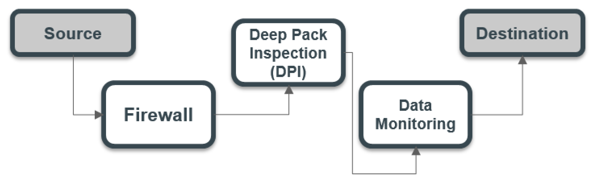
The ‘virtualization’ approach offers advancement through effective deployment of the NFs to the network infrastructures. Network Function Virtualization (NFV) therefore appears as a promising paradigm for solving the above-mentioned problem. The NFV framework decouples the NFs from their dedicated middle-box and deploys them on shared hardware as software. These softwarized NFs, also known as Virtual Network Functions (VNFs), provides network operators with flexibility and agility for embedding and re-embedding of network functionalities. These VNFs are sequentially chained to determine a requested NS, referred to as Service Function Chaining (SFC). Once the SFC is established, the NFV-MANO (NFV Management and Orchestration) embeds the chained VNFs in a specified order onto the substrate nodes, as shown in Figure 1.
NFV-based networks have a few advantages. Firstly, the virtualization of the NFs reduces CAPEX and OPEX. It enables deploying more than one VNF on a single high-volume server, minimizing the hardware purchase and maintenance costs. Secondly, as opposed to the conventional approach, it decreases the implementation time for new network services. This is because of the networks’ availability of high-volume servers. Finally, due to the shift in resource demand, NFV-based networks provide versatile migration of VNFs from one server to another.
Apart from the pros, the NFV-based networks has its own challenges. One of them is ‘NFV-Resource Allocation’ (NFV-RA). An SFC consists of multiple VNFs and Virtual Links (VLs) with diverse resource requirements; these requested resources must be satisfied by the underlying infrastructure for successful deployment. The provisioning of resources by the network for the successful SFCs deployment is called ‘NFV-RA problem’. The main objective of the SFC is to provide promised SLAs to the users, which is accomplished in three stages. In stage 1, an SFC is defined by chaining the VNFs in chronological order (according to the QoS), and this process is called VNFs-Chain Composition (VNFs-CC) [4]. In stage 2, these chained VNFs are optimally deployed onto the substrate nodes subject to certain resource constraints. The graphical representation of the sequentially chained VNFs, which deliver an end-to-end network service is called VNF-Forwarding Graph (VNF-FG). The deployment of these graphs onto the network is called VNF-FG Embedding (VNF-FGE). This VNF-FGE problem is branched out into two sub-problems: Virtual Node (i.e., VNF) mapping and Virtual Link (The connection between two consecutive VNFs) mapping, as illustrated in Figure 2. Stage 3 concentrates on minimizing the VNF-FG’s overall deployment time by providing a time-slotted strategy for the arrival of VNF, this is called VNF Scheduling (VNF-SCH) [4,6]. Our work in this paper is restricted to stages 2 and 3 only, we consider stage 1 as a predetermined factor provided by the network operator.
The VNF-FGE and network dynamism increase the NFV-RA problem’s complexity because of the complicated inter-dependencies between several variables. In fact, the NFV-RA problem is categorized as an NP-Hard problem. This critical problem can be solved using mathematical optimization methods, but at an extreme high computation time [4]. This computational time will scale up exponentially for denser networks. To overcome this, researchers have opted for sub-optimal solutions like heuristics and meta heuristics-based approaches, with a trade-off between the run-time and the global optimal solution. This method is considered a drawback for dynamic systems, where constraints and objectives are continuously varying; it is important to redesign these heuristic models [5].
A zero-touch network can provide an effective placement of the VNF-FGs. Thus, in this work, we are considering Deep Reinforcement Learning (DRL) techniques for the placement of dynamically arriving VNF-FGs. In an environment where the network conditions change vigorously, learning from the past experiences is a beneficial factor for decision-making. In general, the RL approach has been proven to provide better solutions than supervised learning for NP-Hard problems [7]. Additionally, while solving the VNF-FGE problem, we are also examining the performance of the DRL under certain conditions like nodal outages due to disaster or vulnerability, variation in VNF-FGs complexity (i.e., number of VNFs in one forwarding graph), nodal capacity, core capacity and Network (topology) density.
The rest of the paper is organized as follows: Section 2 provides a brief literature review. Followed by the problem formulation of VNF-FGE problem, which is modelled as a Markov Decision Process (MDP) given in Section 3. Section 4 provides an overview of DRL’s functionality and an elaborate description on State Space, Action Space, Environment, and Rewards. Section 5 describes the architecture of Deep Neural Networks, and Section 6 will present a critical analysis of the DRL model. Results and discussions are presented in Section 7. Lastly, Section 8 concludes the paper and additionally provides information about our future plan.
2. Literature Review
Traditionally, the deployment of the NSs is manually performed by the network operator (as mentioned earlier) which is considered as a bin-packing problem which has been studied extensively [5]. To solve the online VNF-FGE problem, various approaches like Integer Linear Program (ILP), and Mixed-Integer Linear Program (MILP) were proposed based on the characteristics of the problem. However, as mentioned in Section 1, achieving the global solution is not affordable because of the increased dynamics and complexity of the networks. Most of the approaches are modelled using the exact method but are implemented for achieving optimal solution, heuristics or metaheuristic algorithms. The researchers have adopted the ILP approach for embedding the VNF onto the network like [8,9]. Few researchers considered some strong assumptions like delay and loss rate induced by links to reduce the computational cost [10], which is not realistic. In [11], the optimization is based on fitness values, i.e., local and global fitness values, where the local values are estimated based on the VM’s availability towards the arrived services, and the global value based on the arrived services structure and resource demand. The authors didn’t consider the entire substrate network rather only a subset to reduce the execution time, casing limitation in the model’s performance. Few authors performed a joint optimization method for VNF mapping and VNF scheduling, which are performed using the MILP model. Achieving the optimal solution for a smaller instance is a not a realistic scenario. However, for dense and complex networks, the authors proposed a heuristic model with a sub-optimal solution with a reduced amount of computation time. Like in [12], the authors adopted a queuing-based model for solving the VNF-FGE problem, where the placement problem is decoupled and performed in a sequential order—that is, starting with the placement of all VNFs of the service on to the substrate nodes and later discovering the physical path based on the propagation delay. However, the authors overlooked the importance of the service acceptance rate with the increase in the topology’s complexity. Applying the -constraint method, the authors [13] modified the multi-objective function into a single objective and proposed a rounding-based heuristic algorithm to reduce the complexity. Some techniques are efficient; nonetheless, they do not assure the best solution and some of the parameters like latency, which is retrieved during the execution time, are not considered.
In [14], the performance of the online mapping and scheduling is evaluated by using three greedy algorithms based on different greedy criteria: Greedy Fast Processing (GFP), Greedy Best Availability (GBA), and Greedy Least Loaded (GLL). Apart from these approaches, the authors proposed a meta-heuristic algorithm called Tabu Search, and this was implemented to eliminate the local minimum solutions by keeping a record of all the previously-visited solutions. The algorithm works on two objective functions: minimizing the flow time of the SFC and minimizing the cost of the resources. The authors have established a firm foundation for the online mapping and scheduling of the VNFs. However, this algorithm is not useful for larger networks due to the iterative process. The authors neglected the virtual link mapping and its corresponding delays. For a more realistic scenario, the consideration of link delay is essential.
In an attempt to solve the above open issue, the authors of [15,16] proposed a model based on Q-Learning (QL). Authors of [15] mainly focus on maximizing the revenue by renting the resources, and this goal is achieved by designing a reward function based on link mapping, where the shortest distance algorithm generates rewards. However, in [16], the authors proposed a joint optimization for both the cloud management system’s orchestration process and monitoring process. The VNFs are clustered together according to the KPIs (say demanded resources) using the unsupervised learning i.e., k-Means clustering algorithm. Based on the VNF’s profile, the placement is performed. The authors of [5] developed a Deep Reinforcement Learning (DRL) based algorithm called Enhanced Exploration Deep Deterministic Policy (). The author compared the performance of with the BtEurope topology and the highly-dense Uninett topology. The performance of Uninett network was compromised as it has higher nodes and links. The VNF embedding is still an open problem for the larger-scale networks. The majority of the existing models considered solving the NFV-RA problem with heuristic or meta-heuristic methods, which provides a sub-optimal solution at reasonable computation time. Thus, a trade-off between the quality of solution and computation time is evident. To improvise these sub-optimal solutions, advance RL models are required. However, the authors [5] claim that mathematical or QL models take an incredibly long time to solve the NFV-RA problem, but they failed to provide their model’s performance in terms of computation time. The authors also neglected to address the overfitting or underfitting problem causes due to the presence of a large number of neurons in the hidden layers. Moreover, the mentioned existing models considered the link allocation between the nodes is according to the shortest-distance technique, causing a highly unbalanced load on particular links making a disruptive topology. A summary of the related works is presented in Table 1, where M, RT, Rel, NodOut, CT, BW, and PD represents Methodology, Resources Type, Relationship between the CPU and RAM, Nodal Outage, Computation Time, Bandwidth and Propagation Delay respectively.
In our previous work [17], we have considered the QL model for solving the VNF-FGE problem. QL is a robust off-policy model-free algorithm but practices an iterative method to achieve the solution, causing the degradation in the performance with the increase in the network complexity and density. In order to achieve the optimal solution, the computation rate was high. Thus, this paper is an advancement of our previous work.
In this paper, we have adopted DQL for solving the VNF-FGE problem. This framework addresses the following issues: (1) the overfitting or underfitting problem caused by neural networks with larger neurons in the hidden layers; (2) by obtaining a better sub-optimal solution under reasonable computational time; (3) maintaining an equilibrium throughout the topology by choosing a much realistic link selection approach where the biases towards specific links are eradicated; and (4) we have considered a more realistic relationship between the CPU and RAM (nodal resources) rather than random resource initialization. This framework has been well examined for the nodal outage, which previously none of the research has performed; moreover, we have done a thorough investigation of the VNF complexity, nodal capacity (horizontally and vertically) explained in the later sections. This is an early-stage work on studying DQL models’ robustness on different network topologies with full or partial topology information. To improvise the performance, we have proposed a Human-centered DQL model. Towards that goal, here in this paper, we present some simulation results for estimating the performances of compromised networks where the nodal outages occurred due to disasters.
3. VNF-FG Problem Formulation
In this section, we will describe the objective and constraints used to construct an optimization problem. Our optimization problem mainly focuses on solving the NFV-RA issue. Moreover, the constraints are organized into five parts: virtual node (VN) mapping, nodal balance, virtual link (VL) mapping, seamless path, and finally latency.
3.1. Constraints
3.1.1. VN Mapping
As we know, each VNF-FG is a graphical representation of a set of VNFs and VLs along with its resource requirements. Depending upon the service type, each VNF requirement varies. Some VNFs like Firewall and Deep Pack Inspection demand more central Processing Unit (CPU) and RAM resources, others comparatively less. Likewise, these requested resources can be CPU core, RAM, Memory, etc. One of the critical aspects for a successful VNF deployment is the provisioning of sufficient resources by the substrate nodes, according to the requested resources. Thus, the first constraint will check the availability of the resources for the VNFs in the substrate network (Here, onward ‘Substrate Network’ or ‘Topology’ represents the Telecommunication Network.),
where indicates the amount of requested resource r by the VNF v, and represents the availability of resource r on the substrate node (i.e., the node present in the substrate network) h. is a binary variable, which indicates the placement of the v VNF onto the h substrate node. If = 1, this indicates the successful placement of VNF onto the selected substrate node, else = 0 represents an unsuccessful placement of VNFs, leading to an eviction of the corresponding VNF-FG.
3.1.2. Nodal Balance
In order to prevent any rise of unpredictable conditions, it is essential to establish an equilibrium on the substrate network. Placing all VNFs of a VNF-FG on a single substrate node will cause an overload on them as well as on its corresponding substrate links. This will lead to an inadequate performance by the networks. Thus, it is crucial to deploy the VNFs of a VNF-FG onto different substrate nodes, which will be the second constraint. This constraint ensures that only one VNF from a particular VNF-FG is embedded in a substrate node. Note that other VNFs from other VNF-FGs can also be embedded on the substrate node in question, but, for every instance of a VNF-FG, only one VNF belonging to it will be embedded on a particular substrate node:
3.1.3. VL Mapping
Not only it is essential to verify the availability of the substrate nodes during the placement of the VNFs, but it is also vital to assess the availability of the links. Thus, the SFC can provide promised QoS support to the users. This is why improper VL mapping can trigger poor network performance. The third constraint, therefore, focuses on the links and their resources. A successful deployment of the VL is achieved when the substrate link satisfies the demanded link requirements like bandwidth and latency. Therefore, for bandwidth resources,
where indicates the requested bandwidth b by the VL m, and represents the availability of bandwidth b on substrate link n. indicates the placement of VL m onto the substrate link n.
3.1.4. Seamless Path
After the deployment of the VNFs and their VLs onto the substrate network, a continuous path between the head VNF and end VNF needs to be established. To avoid any loop formation in the discovered path, we adopted constraint 7 from paper [5], i.e.,
where and are the outgoing and incoming links from the node h. H and M are the set of substrate nodes in a network and set of VL in a VNF-FG, respectively.
3.1.5. Latency
Our work focuses on the latency-sensitive application, where the selection of a candidate path for a VL m is based on the latency criteria,
where is 1 when VL m is embedded on substrate link n. is the latency of substrate link n, and represents the set of all possible physical links that forms a candidate path for VL m.
We are representing the successful deployment of the VNF-FG in terms of a unit step function . The mathematical representation of a successful VNF-FG J placement is given by
where = 1 when x ≥ 0, else = 0 if x ≥ 1, and is the total number of VNFs present in VNF-FG.
3.2. Objective
The objective of the constructed model is to maximize the service acceptance rate (SAR); that is, maximizing the number of VNF-FGs placement onto the substrate network.
If all the chained VNFs of a VNF-FG are deployed onto the substrate nodes by satisfying the above constraints (Equations (1)–(5)), then it is called a successful VNF-FG deployment. Once a VNF-FG is successfully embedded, then the algorithm selects the next VNF-FG for the implementation. In the next section, we will describe our approach to solve this NP-Hardness problem.
4. Deep Reinforcement Learning
4.1. Reinforcement Learning
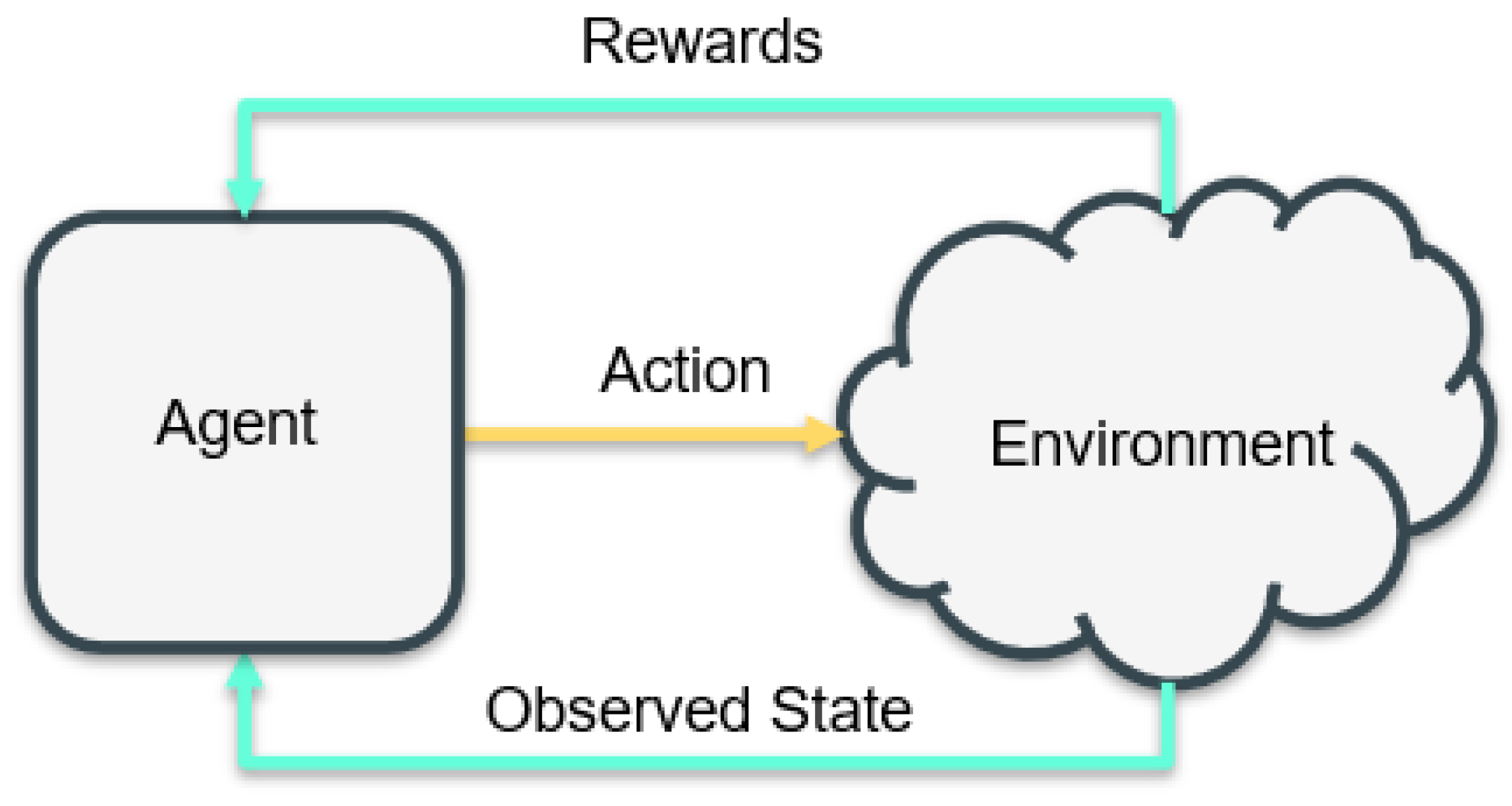
Reinforcement Learning is a learning process where, at each time-step, the agent observes a state S, and, accordingly, an action A is executed. Based on this action, the environment provides reward and the next state, as shown in Figure 3.
From the obtained observations (i.e., rewards and next state), the agent’s goal is to improvise the decision strategy for achieving an optimal policy to attain an optimal solution. In other words, RL is a self-learning process where the models are trained with the help of online data, where these models optimize the problem by accumulating the rewards from the environment and avoiding receiving any penalties. These trained models will maintain the performance even during the network dynamism. In our work, we formulated the optimization problem in terms of the Markov Decision Process (MDP) because MDP establishes a mathematical structure for examining the decision-making problems, this decision-making process is partially random and supervised by the agent. Thus, the RL technique uses MDP framework for solving the optimization problem [18]. RL’s main aim is to find an optimal policy for the decision-maker (agent). This optimal policy for a state is obtained by maximizing the optimal action-value function, i.e.,
This action-value function is estimated using the Bellman Equation, i.e.,
, , and are the state, action, and reward obtained at time-step t, respectively. Moreover, and are the state and action for next time-step, and is the probability of next state and reward for a given current state and action. In addition, is the probability of selecting the next action under a policy with the discounting factor.
However, to estimate the optimal action-value, the most efficient and commonly used literature approach is Q-Learning (QL) [10]. QL is an off-policy model-free algorithm, where the Target policy (This policy is used to estimate the action-value by the agent.) learns from the Behaviour policy (This policy is used for choosing an action by the agent.) to achieve an optimal solution.
Thus, Equation (9) is modified as
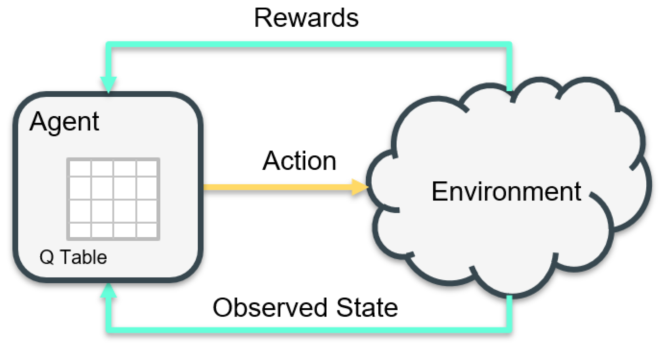
under the policy. In other words, the action-value (also known as Q value) is defined as an expected discounted reward when an action is executed for a state under a policy. QL agent intends to explore the unknown environment by executing an action at each time-step for the observed state. The learned values are stored in a form of table called a Q-table as shown in Figure 4. These Q-table values provide crucial information about the state–action pair, which supports in discovering the best action for the current state. Thus, the Q value is estimated in an iterative process, which will be effective for smaller-scale space but not for larger-scale space due to the curse of dimensionality [19].
In order to address the problem, Deep Reinforcement Learning (DRL) is implemented, where the Q-table is replaced with the Deep Neural Network (DNN) to approximate the Q values, as seen in Figure 5. RL is considered to be unpredictable or highly prone to divergence where a nonlinear function approximator such as a neural network is used to represent the Q-value function. This divergence is due to the correlation between the transitions, where a trivial variation to the Q value can impact the policy, causing a substantial effect on the Q value and target value [20]. This effect is due to the correlation of the Q value with the target value, where both values are estimated using the same set of parameters, as shown in Figure 6.
Thus, the absence of this correlation will resolve the instability between them. This can be accomplished by incorporating the Target Neural Networks, and Experience Replay, which are addressed in the upcoming sections.
4.2. Target Neural Networks
The DQL creates a correlation between the Q-value and Target value, causing destabilization in the algorithm. Instead of using only one neural network (NN), Primary NN, to estimate the Q values and Target value, the authors in [20] proposed Target NN to evaluate the Target value (or can say to learn the Target policy). This Target NN consists of the same architecture as Primary NN; however, the parameters (i.e., weights and bias) are updated periodically (much smoothly), say after every iterations. In other words, after every iterations, the primary NN parameters are copied to target NN, minimizing the correlation between them and achieving a stable algorithm. Due to this stability, the performance of the model will improve. The architecture of modified DQL model with Target NN is shown in Figure 7 and Figure 8:
4.3. Experience Replay
Experience Replay is a process of storing the observed transitions like state, action, rewards, next state, in a memory buffer. From the memory buffer, these stored transitions are uniformly sampled, i.e., all the transitions are considered equally important. The experience replay will randomly pick a transition set to train the model by limiting the correlation between the transitions. Thus, using Experience Replay, the correlation between transitions can be prevented.The functionality of the Experience Replay has been demonstrated in Figure 9.
4.4. Environment
We have assumed the environment of DRL as the physical topology, where the VNF will be deployed. The physical topology is comprised of high-volume servers with defined processing resources. We modelled the topology as an undirected graph , where H and N represent the topology’s nodes and links, respectively. Each node consists of resources like CPU core, RAM, Memory, etc. Similarly, each link will be comprised of resources like bandwidth, latency, loss rate, etc.
The environment is the physical network infrastructure owned by the network operators.
4.5. SFC Arrival
We consider a discrete time-step (i.e., time-slotted) technique for the arrival and departure of the SFCs defined by the service provider. At the beginning of each time-step, the arrived SFC is deployed onto the substrate network. However, the SFC will be rejected on an unsuccessful deployment by the substrate at the end of a time-step.
4.6. State Space
Each requested NS is graphically represented as a VNF-FG, which is a directed graph . This VNF-FG is comprised of VNFs and VLs with their respective resource requirements, which is represented as + . and represent the number of VNFs and VLs in a VNF-FG, respectively. and indicate the resource requirement by the VNFs and VLs, respectively. We are assuming that VNFs and VLs request for a definite amount of CPU core, RAM, bandwidth, and latency. We have considered the state space as the specifications of the VNF-FG, where this detailed description of the state is fed to the DQL agent. Based on this description, the DQL agent will provide the best solution (optimum solution) in terms of action.
In terms of the resource initialization, a few researchers have arbitrarily allocated the resources, ignoring the fact that resources like CPU core and RAM are strongly correlated. Thus, in our work, we are adopting the relationship between CPU and RAM as provided in [21], that is, each node will contain a certain number of CPU core along with its RAM requirement.
4.7. Action Space
In our model, we define the action space as the total amount of nodes present in the topology, for each VNF of a VNF-FG. Thus, the size of the action space per VNF-FG is .
With the implementation of the VNF-FGs onto the substrate network, the availability of the substrate nodes is also altered, making a few nodal resources almost depleted. The selection of such kind of nodes can degrade the performance of the model; the higher the availability, the better performance that can be expected. Therefore, we have constructed a heuristic model where a node’s prioritization is based on the available nodal capacity that is represented by the corresponding weight variable . Thus, a node with higher available resources has a better probability of being picked (providing a higher chance of satisfying the VNFs). Algorithm 1 demonstrates the proposed heuristic model.
| Algorithm 1: Action space exploration |
 |
4.8. Reward Function
The environment rewards the agent only if the selected action enables a successful placement of the VNFs and VLs; otherwise, a penalty is assigned to the agent. We have considered two types of rewards: local and global rewards. The local reward is given when the agent provides a satisfactory substrate node per VNF and substrate link per VL. The global reward is given when a VNF-FG is successfully deployed (i.e., a continuous path between the head and end VNFs is defined subject to latency and other constraints).
In the literature, most researchers considered the Shortest-Distance algorithm to establish the path between the VNFs; adopting this technique will cause biases leading to high congestion on a few links, which will generate a prolonged link delay. This method will not be feasible for delay-sensitive applications. Thus, we adopted an approach where the path per VNF-FG is established based on the upper bound of the latency. We have set this limit to 30 ms in our analyses. Thus, the reward function is constructed based on the deployment of the VNFs and VLs onto the satisfying substrate nodes and links, respectively. In addition, the reward function ensures that the communication delay between the two VNFs should not exceed the upper bound of the latency. The algorithm for the placement of link is provided in Algorithm 3. Algorithm 2 summarises our model for VNF-FG embedding. We have examined the performance of this model under several scenarios like different network topology, nodal capacity, core capacity, and diverse nodal-outage levels. Thus, we have generated several results based on the network conditions, some of them being presented in the next section.
5. Deep Neural Network
The architecture of the NN is controlled by two hyper-parameters: (1) the number of hidden layers W; i.e., the depth of the NN, and (2) the number of neurons in each hidden layer; i.e., the width of the NN, since W’s best value cannot be discovered using any analytical calculation but rather a systematic experiment. Thus, this segment discusses the impact of W in our model where these hidden layers are fully connected with a drop probability of 0. We are considering a wide range of W ranging from 2 to 10 layers.
Recalling the Primary and Target NNs, these NNs are composed of the same architecture; thus, W’s change will influence both NNs. To examine this performance, we have considered the Netrail Topology, where the deployment of 100 VNF-FG per episode will occur. Furthermore, we assumed that each VNF-FG is comprised of three VNFs with diverse resource requirements. This experiment is repeated for various Nodal capacity, i.e., 2, 4, 8, and 12 Core CPU, as well as Core capacity (2, 4, 8, and 16 VNFs per Core), as shown in the Figure 10. The obtained results are evaluated in terms of the Runtime and Service Acceptance Ratio (SAR), as shown in Figure 10 and Figure 11, respectively.
| Algorithm 2: VNF placement based on DQL |
 |
With the increase in W, the complexity of the NNs intensifies, resulting in elevated Runtime to solve the problem. Thus, when , it takes ∼27 s longer to deploy 4 more VNF-FGs (per Run where, 1 Run = 100 Episodes) than . Further escalation in the Runtime happens with the increase in Nodal capacity and Core capacity. We have considered a model with two hidden layers because provides roughly the same average SAR per Scenario as compared with a higher degree of W, at lower Runtime, as presented in Figure 11.
| Algorithm 3: Virtual Link Placement |
 |
In this section, we examined how the NN parameters affect the VNF-FG embedding. The remaining results are presented in Section 7.
6. Critical Analysis
This section will present a summary of the challenges that occurred during the construction of the DRL model. As mentioned earlier, the DRL model was constructed only with one NN, i.e., primary NN, which learns both the behaviour policy and the target policy to solve the NFV-RA problem. The usage of the primary NN’s weights and biases (parameters) for determining two distinctive tasks causes highly unstable results. That is, the target values obtained from the primary NN constantly wavered over the iterations; this results in unstable learning.
Thus, to provide stability in the learning, the DRL model’s performance was improvised using the target NN and Experience Replay method. To enhance the performance further, we have used a heuristic model. The model’s foremost purpose is to prioritize the nodes based on the available nodal capacity in the topology; by doing so, we have increased the chance of successfully embedding of the arriving services. For example, in the case of 2 core CPU and 16 VNF per core for 3 VNF per service, the average SAR for a single NN DQL model was 69.83, whereas, with the improved version of the DRL model, the average SAR was escalated to almost 74 for Netrail topology. The single-NN-DRL model’s SAR over each episode ranged from 65 to 73 SAR (i.e., [69, 69, 68, 72, …, 69, 72, 69, 70, 70]), showing high placement instability; however, this trend of high fluctuations over the episodes is not shown in the adapted DRL model, making an assurance of stability in learning.
DRL models have a tendency to encounter the overfitting or underfitting problem. These issues or problems are avoided by incorporating techniques like, firstly, the Greedy method to estimate the action per state. Based on the probability of , the model will either choose the action randomly or based on the maximum Q value–secondly, introducing a regularization method called Dropout. Here, the neurons are randomly assigned as inactive neurons in the hidden layers. This randomness is based on the probability of dropout (p); in our model, we have considered p as 0.2. This makes learning in a sparse NN, reducing any overfitting. Moreover, experience replay also lessens any overfitting problem as it breaks the correlation between the transitions.
7. Simulation Results
We have successfully constructed the DRL model for solving the VNF-FGE problem with and without the nodal outages. Currently, in this paper, we considered two distinctive topologies as our environment: Netrail topology with 7 Nodes and 10 links and BtEurope topology with 24 Nodes and 37 links [22]. The performance of the model is evaluated based on the SAR, and Runtime, under diverse conditions: (1) Variation in Nodal capacity, (2) Variation in VNF-FG complexity, and (3) Nodal outages. A diagrammatic representation of these expansions is shown in Figure 12.
We assumed that the link capacity of the substrate network is between 1 Gbps to 10 Gbps, and the link delays of 0 to 10 ms, which is initialized randomly among the links. Note that, when we embed the VNF-FGs into the substrate network, we need to ensure that a path between any two VNFs should have a total delay of less than 30 ms, which is a sum of these randomly initialized link delays. We have started by analyzing the performances of the networks based on the different nodal capacity. For each run, we have considered one scenario out of four: 2, 4, 8, and 12 core CPUs per node where each core can accommodate 2, 4, 8, and 16 VNFs. Therefore, we have evaluated the network performance for 16 different combinations of nodal capacity.
To advance our work, we have investigated the performance of the model for various degrees of complexity of the VNF-FGs. That is 2, 4, 6, 8, and 10 VNFs per VNF-FG. These VNF-FGs are generated using the Erdős–Rényi model [23] with the value of 0.3. The probability of connectivity among the VNFs depends upon the value and number of VNFs per VNF-FG. Thus, these VNF-FG’s degree of complexity varies. However, our investigation did not end here; we have examined the efficiency of the Intelligent topology under the compromised situation by assuming the occurrence of nodal outage due to disasters or vulnerability. The above experiment is analyzed for 30 ms delay with 30% and 50% of the nodal outages.
Each run consists of 100 episodes, and each episode comprises 100 time-steps. Each time-step generates one VNF-FG with a unique combination of resources. The DRL model is built using the PyTorch library written in the Python language. The results are generated using the Intel Core i7 processor with 64 GB RAM. The following Table 2 provides the parameters used to construct the DRL model. The constructed codes for the DRL model are available in a repository [24].
7.1. Service Acceptance Ratio
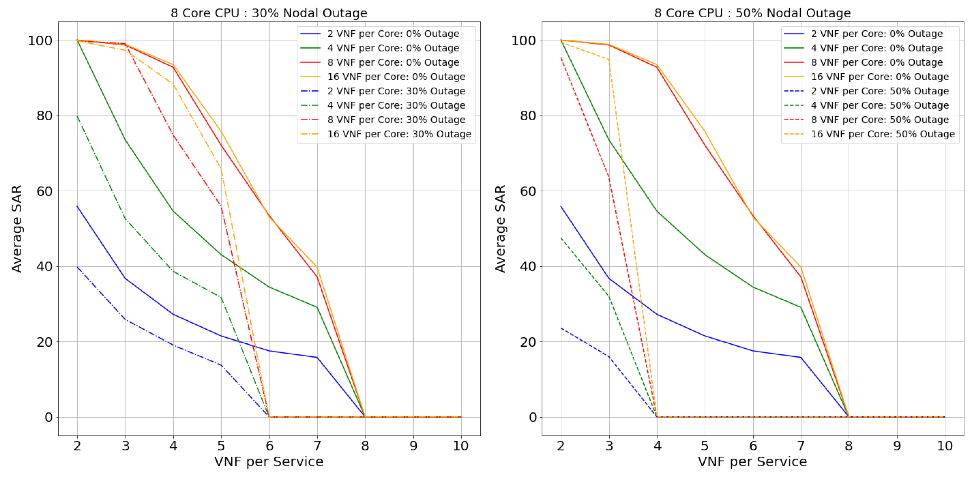
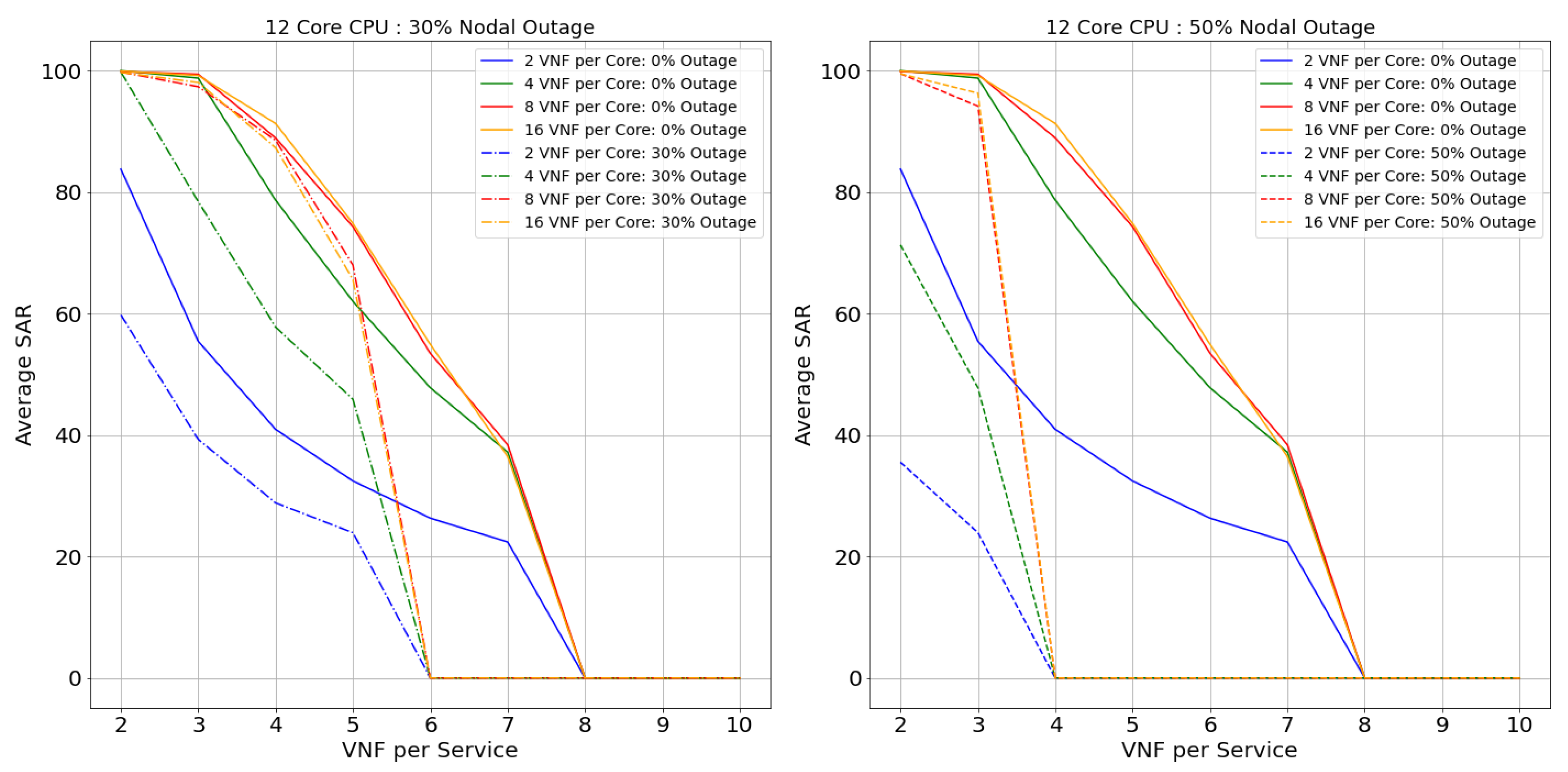
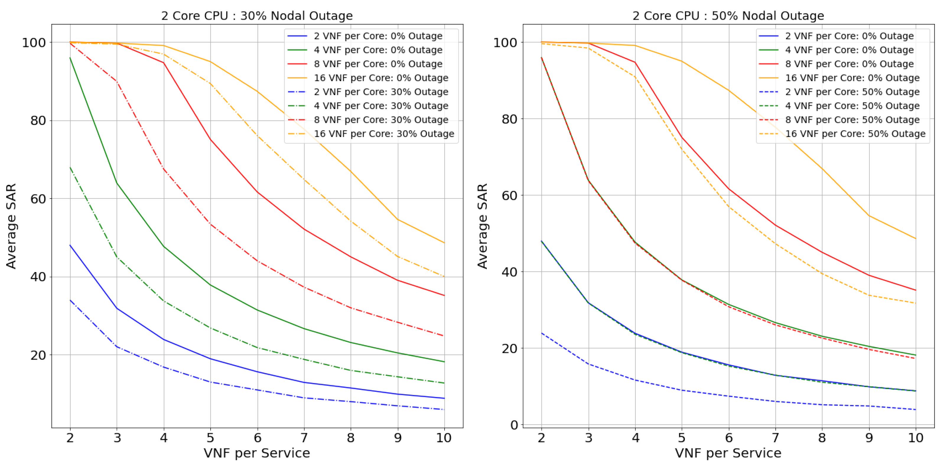
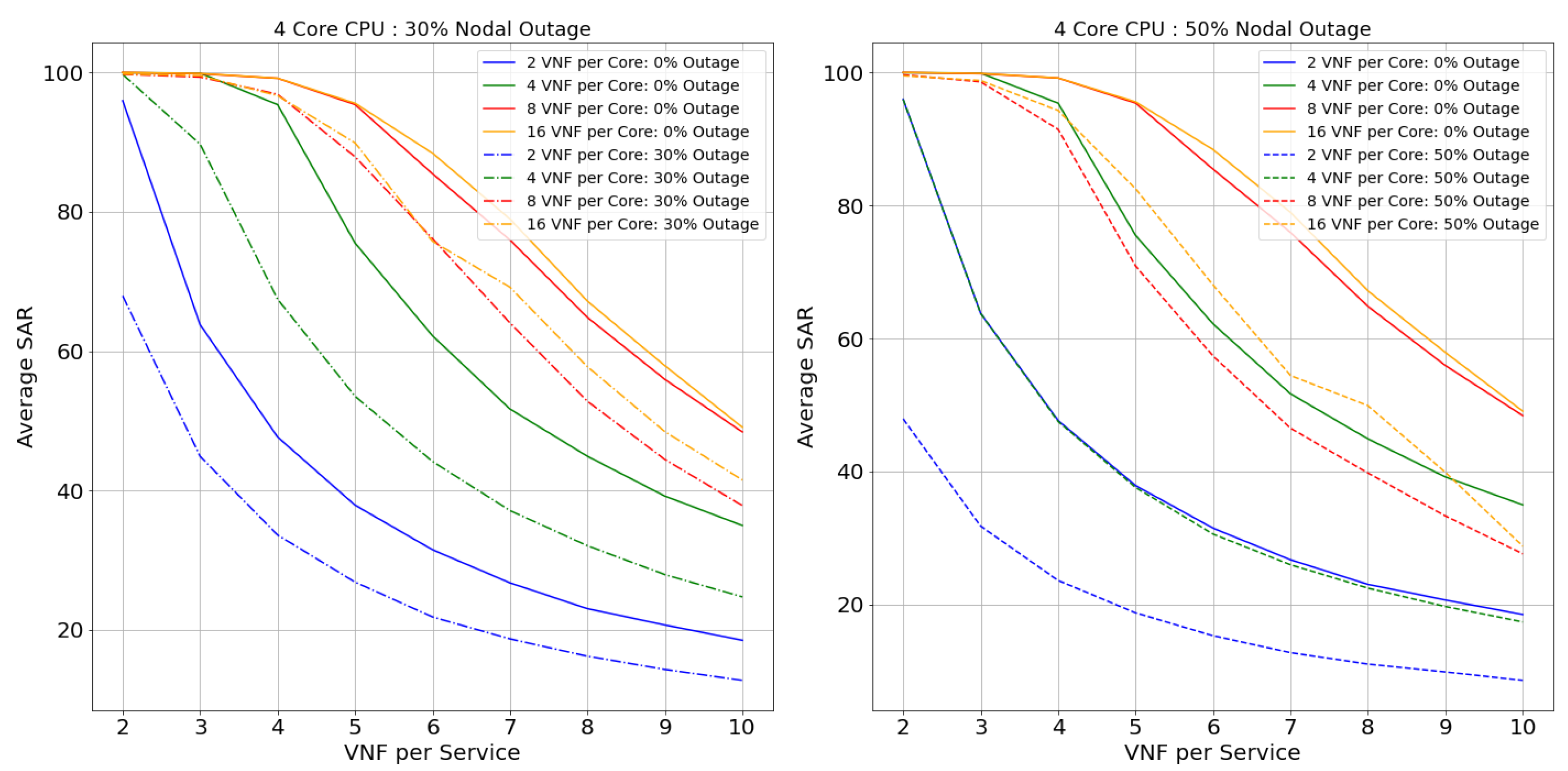
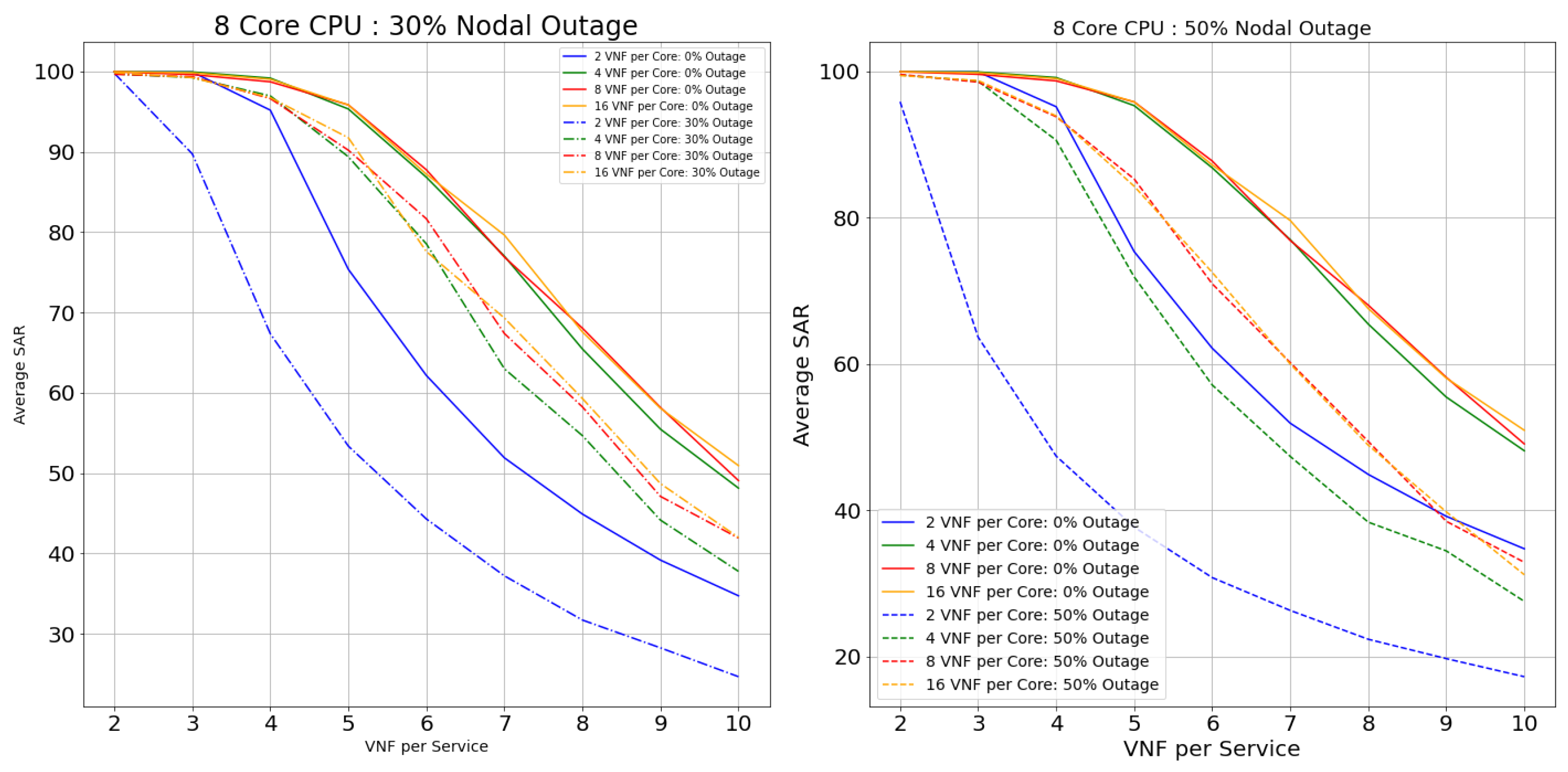
Netrail topology’s performance is represented from Figure 13, Figure 14, Figure 15 and Figure 16 for 2, 4, 8, and 12 core CPUs, respectively. Figure 17, Figure 18, Figure 19 and Figure 20 illustrate the performance of the BtEurope topology for 2, 4, 8, and 12 core CPUs, respectively.
Considering the performance of topologies with 0% of nodal outage from the Figure 13, Figure 14, Figure 15, Figure 16, Figure 17, Figure 18, Figure 19 and Figure 20, we can state that, with the rise in the core capacity (i.e., 2, 4, 8, and 16 VNF per core) as well as nodal capacity (i.e., 2, 4, 8, and 12 core), the SAR of the topologies increases. This is due to the surge in resource availability. These highly available resources are still inadequate with the increase in the VNF-FG’s complexity (i.e., VNFs per VNF-FG). The rise in the complexity induces a surge in VNF’s resource demand, causing these highly available resources to be insufficient. For a smaller topology like Netrail, the model refuses deployment of all VNF-FGs after a certain point, like 8 VNFs per service for 0% nodal outage, as shown in Figure 13. This is due to the constraint depicted by Equation (2), which states that each substrate node can accommodate just one VNF, and Netrail topology consists of only seven nodes. Any VNF-FGs containing VNFs more than the total number of substrate nodes are rejected. Therefore, small topologies dismiss the complex VNF-FGs. This is not the case for the large topology like BtEurope where a sufficient amount of resources are available for the placement of the VNF-FGs, making sure that the constraint in Equation (2) is always satisfied. Because of the high availability of resources, the BtEurope’s performance is much better than Netrail. For example, considering the lowest available resource scenario: 2 core CPU and 2 VNF per core (see Figure 13 and Figure 17), the SAR for BtEurope is approximately 50%, whereas Netrail could only serve ∼15% of VNF-FGs.
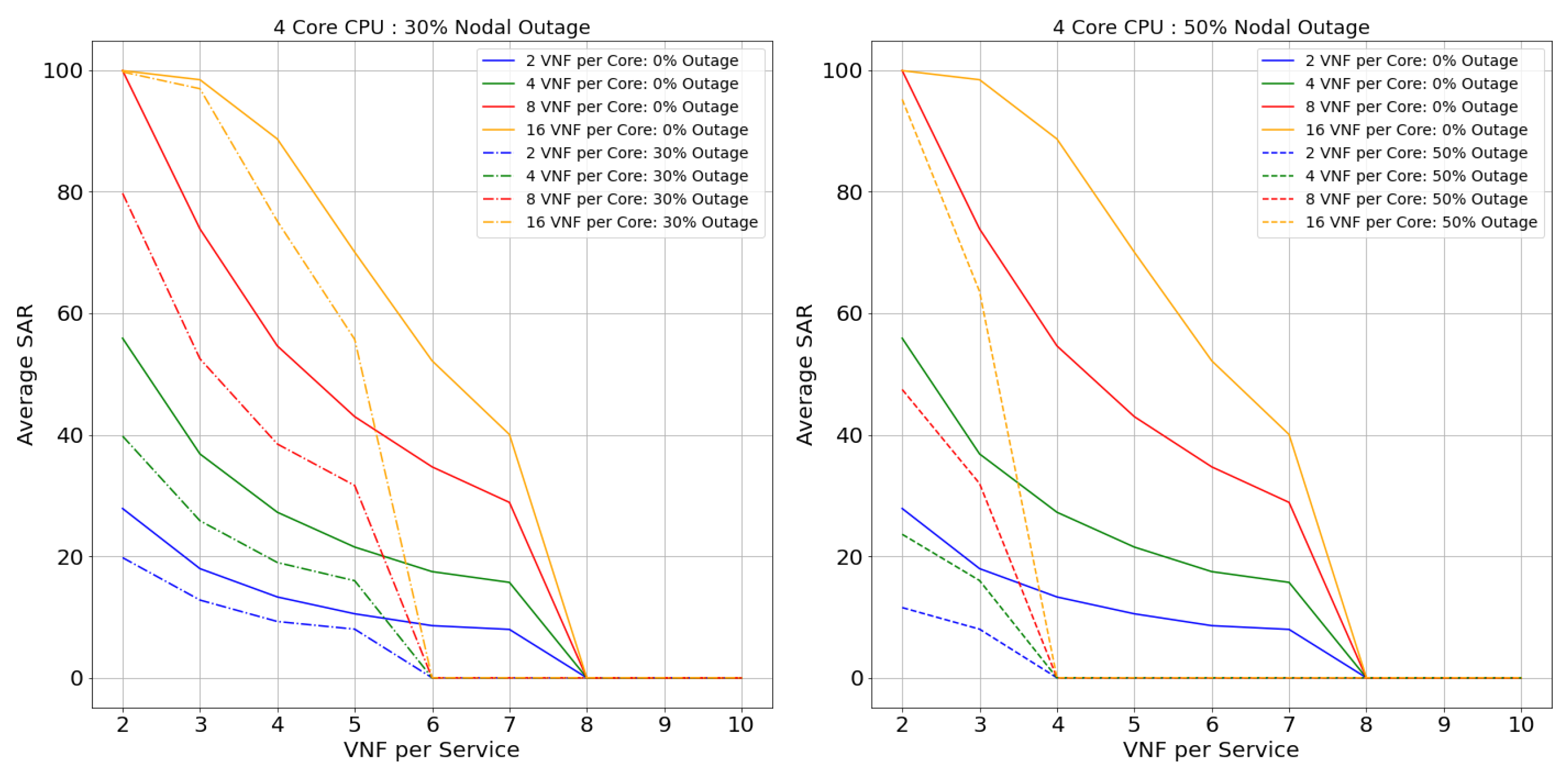
Now, we focus our discussion on the Netrail topology’s performance with 30% and 50% nodal outage. For two VNFs per service (or two VNFs per VNF-FG. We have used the terms ‘VNF per service’ and ‘VNF per VNF-FG’ interchangeably), all arrived VNF-FGs are accepted at 0% outage. With the rise in the nodal outage, this SAR declines due to less availability of substrate nodes. For example, for 30% nodal outage, the SAR is dropped by 20% (see Figure 13). If we examine the performance of the model horizontally (i.e., along with the VNF-FGs complexity), the rejection rate increases. This performance is maintained till the resource is exhausted or the constraint in Equation (2) is not satisfied. For 50% of the nodal outage, i.e., when the topology is modified and is composed of only three nodes, there is an acceptance of only fewer VNF-FGs (see Figure 15 and Figure 16, which show that the 8-core and 12-core cases perform better than the 2-core and 4-core cases in the presence of nodal outage due to the presence of more resources in the topology). Exploring horizontally in the Figure 13 and Figure 15, the model’s performance deteriorates slowly due to the resource depletion, especially the link availability. The probability of connectivity of links between the VNFs is based on number of VNFs per Service. With the increase of VNF’s per service, the demand for link resources increases.
In BtEurope, with the increase in the nodal capacity, the model’s performance for the 4, 8, and 12 VNF per CPU (see Figure 18, Figure 19 and Figure 20) has been satisfying. Especially considering 12 core CPU, even for the outage topology, the placement of VNF-FGs are substantially better than the remaining scenarios. However, we have also seen that the link resources deplete quickly with the increase in the VNF-FG’s complexity as in Netrail. However, the resource exhaustion rate for BtEurope is much slower than the Netrail.
In conclusion, the SAR for the larger topology was much better than a smaller topology, solely because of its ample resource availability. Overall, two VNF per core CPU always showed the worst performance, whereas 8, 16 VNF per core CPU could accommodate a maximum amount of VNF-FGs until the resources were consumed or constraints in Equation (2) were unsatisfied.
7.2. Runtime
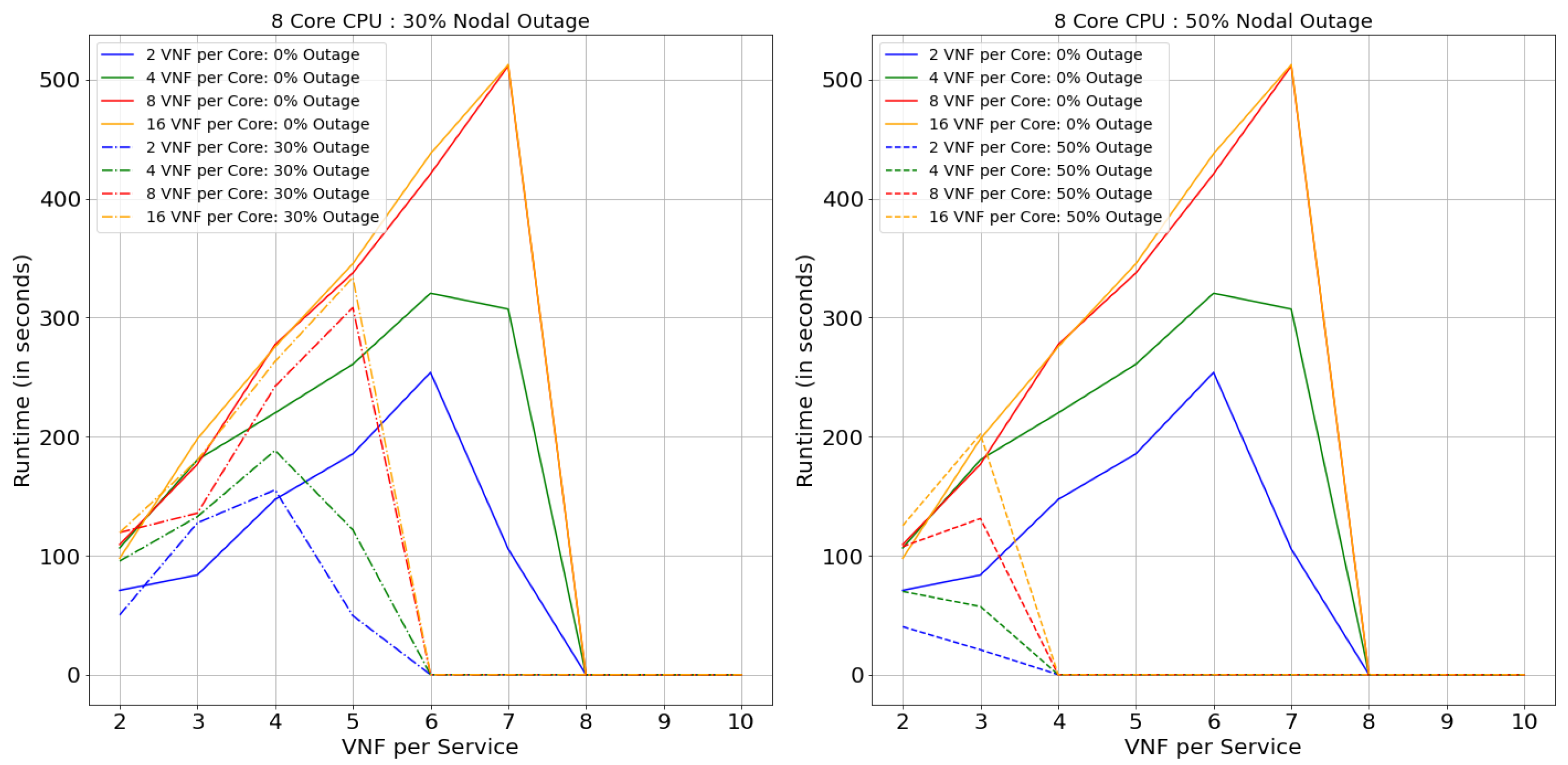
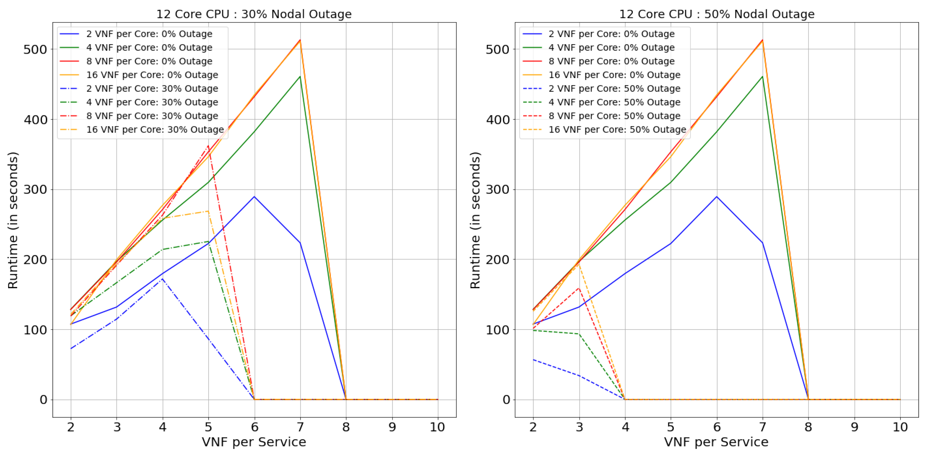
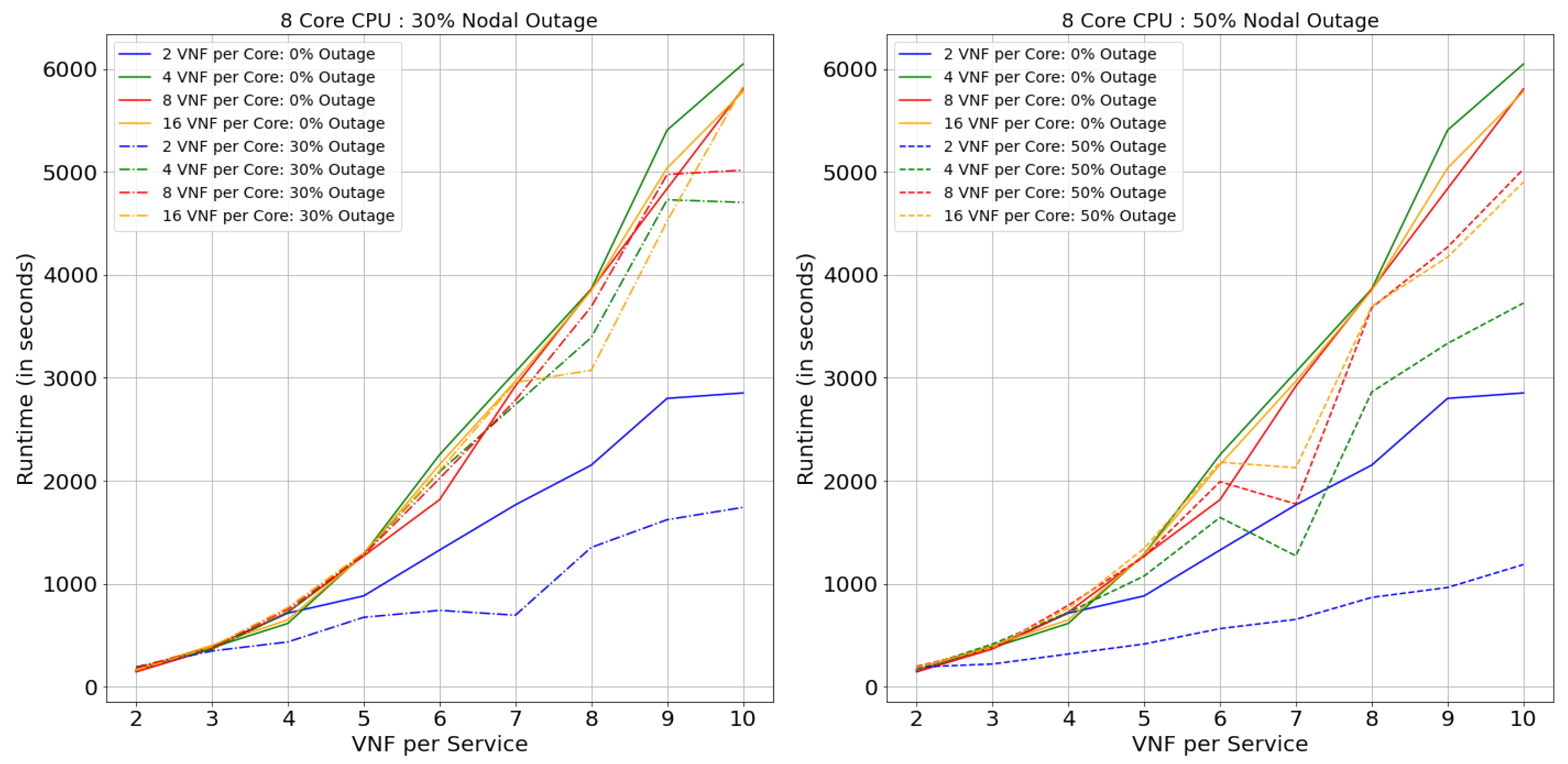
This section will describe the performance of the model in terms of Runtime (computation time). Figure 21, Figure 22, Figure 23 and Figure 24 illustrate the performance of Netrail topology and Figure 25, Figure 26, Figure 27 and Figure 28 for BtEurope topology, under specified conditions. In general, it is evident from the figures that, to solve the VNF-FGE problem, BtEurope needs more significant computation time than Netrail. For example, BtEurope took ∼6× more computation time than Netrail to embed VNF-FGs for 12 Core CPUs with 16 VNF per Core and 7 VNF per Service (see Figure 24 and Figure 28). This increase in computation time is due to the extensiveness of the BtEurope topology.
We also evaluated the consequence of the model’s performance, during the expansion of core and nodal capacity. From the results, we can articulate that the computation time also increases with the increase in the core capacity per substrate node. For instance, considering the performance of 2 VNF per service case for 4 Core CPU with 2 VNF per core and 8 VNF per core (see Figure 22), we found that higher core capacity (i.e., 8 VNF per core) took an additional 2.5× computation time for the placements; this summary is for Netrail topology without any outage. This similar effect is observed in BtEurope topology with an increase of 6× computation time due to higher core capacity (7 VNFs per Service, 2 core CPU, 16 VNF per Core compared with 4 VNF per Core) (see Figure 25). This similar variation can be seen among the increase in nodal capacity.
Likewise, a similar effect can be witnessed, with the increase in the VNFs per VNF-FG, the VL connection’s complexity also escalates. Thus, it takes a more prolonged time to find an optimal link placement solution, by satisfying the upper bound on latency. However, we observe that there is an abrupt drop in the Runtimes as a general trend in all the runtime-related plots. As mentioned in the SAR section, this is because the smaller topologies are incapable of satisfying the constraint in Equation (2), causing rejection of all arriving VNF-FGs.
We also observed that the model requires less time to find the optimum solution in terms of the nodal outage than without outage topology. This is solely due to the topology’s connectivity decrease with the increase in the nodal outage percentage. Consider a 2-Core CPU case with 16 VNF per Core and 10 VNF per Services. In BtEurope topology without any outage, the model successfully embeds 25 more VNF-FGs than for 50% of nodal outage topology, but at the cost of an additional 1300 s runtime (see Figure 25).
On the comparison between the topologies, the Netrail Runtime is generally smaller than BtEurope. This is because, for a small topology, the action space is within the range of 7, which causes a faster search to obtain the optimal solution. However, for a dense network like BtEurope, where the action space is much larger; this generates a more massive investigation to find the optimal solution.
8. Conclusions and Future Work
In conclusion, we have proposed to solve an NP-Hard problem: NFV-RA, using deep Q-learning (DQL) models. An extensive investigation of DQL’s performance under diverse conditions of network density, nodal and core capacity, nodal outage, and VNF-FG complexity is performed. The DQL agent discovered the characteristics of the topologies under specifying conditions and provided near-optimal solutions. To improve performance, we have introduced a heuristic model for better exploration of the action space. In our results, with the increase in network density or nodal capacity or VNF-FG’s complexity, the model took extremely high computation time to execute the desirable results. Moreover, with the rise in complexity of the VNF-FG, the resources decline much faster. In terms of the nodal outage, for specific topologies and particular combination of resources, we have achieved between 70–90% SAR even with a 50% nodal outage but at the cost of high computation time.
This performance can be improved further by introducing a model-free, actor-critic algorithm known as the Deep Deterministic Policy Gradient (DDPG), which deals with larger action spaces. In our future work, we will present a thorough study of the DQL model using DDPG under the specified complex circumstances.
Author Contributions
Funding acquisition, A.N.; Supervision, A.N., H.A.; Modelling and Simulation, S.B.C.; writing—original draft preparation, S.B.C.; writing—review and editing, A.N., S.S., H.A. All authors have read and agreed to the published version of the manuscript.
Funding
This work was funded by UCD School of Electrical and Electronic Engineering (Project Code R20813; Cost Center 4077).
Data Availability Statement
All data used in this work were obtained from open-source, publicly-available repositories.
Conflicts of Interest
The authors declare no conflict of interest.
References
- Saad, W.; Bennis, M.; Chen, M. A vision of 6G wireless systems: Applications, trends, technologies, and open research problems. IEEE Netw. 2019, 34, 134–142. [Google Scholar] [CrossRef] [Green Version]
- Mijumbi, R.; Serrat, J.; Gorricho, J.L.; Bouten, N.; De Turck, F.; Boutaba, R. Network function virtualization: State-of-the-art and research challenges. IEEE Commun. Surv. Tutor. 2015, 18, 236–262. [Google Scholar] [CrossRef] [Green Version]
- Letaief, K.B.; Chen, W.; Shi, Y.; Zhang, J.; Zhang, Y.J.A. The roadmap to 6G: AI empowered wireless networks. IEEE Commun. Mag. 2019, 57, 84–90. [Google Scholar] [CrossRef] [Green Version]
- Herrera, J.G.; Botero, J.F. Resource allocation in NFV: A comprehensive survey. IEEE Trans. Netw. Serv. Manag. 2016, 13, 518–532. [Google Scholar] [CrossRef]
- Quang, P.T.A.; Hadjadj-Aoul, Y.; Outtagarts, A. A deep reinforcement learning approach for VNF Forwarding Graph Embedding. IEEE Trans. Netw. Serv. Manag. 2019, 16, 1318–1331. [Google Scholar] [CrossRef] [Green Version]
- Nejad, M.A.T.; Parsaeefard, S.; Maddah-Ali, M.A.; Mahmoodi, T.; Khalaj, B.H. vSPACE: VNF simultaneous placement, admission control and embedding. IEEE J. Sel. Areas Commun. 2018, 36, 542–557. [Google Scholar] [CrossRef] [Green Version]
- Quang, P.T.A.; Bradai, A.; Singh, K.D.; Picard, G.; Riggio, R. Single and multi-domain adaptive allocation algorithms for vnf forwarding graph embedding. IEEE Trans. Netw. Serv. Manag. 2018, 16, 98–112. [Google Scholar] [CrossRef]
- Luizelli, M.C.; Bays, L.R.; Buriol, L.S.; Barcellos, M.P.; Gaspary, L.P. Piecing together the NFV provisioning puzzle: Efficient placement and chaining of virtual network functions. In Proceedings of the 2015 IFIP/IEEE International Symposium on Integrated Network Management (IM), Ottawa, ON, Canada, 11–15 May 2015; pp. 98–106. [Google Scholar]
- Chowdhury, S.R.; Ahmed, R.; Shahriar, N.; Khan, A.; Boutaba, R.; Mitra, J.; Liu, L. Revine: Reallocation of virtual network embedding to eliminate substrate bottlenecks. In Proceedings of the 2017 IFIP/IEEE Symposium on Integrated Network and Service Management (IM), Lisbon, Portugal, 8–12 May 2017; pp. 116–124. [Google Scholar]
- Xie, Y.; Liu, Z.; Wang, S.; Wang, Y. Service function chaining resource allocation: A survey. arXiv 2016, arXiv:1608.00095. [Google Scholar]
- Dehury, C.K.; Sahoo, P.K. DYVINE: Fitness-based dynamic virtual network embedding in cloud computing. IEEE J. Sel. Areas Commun. 2019, 37, 1029–1045. [Google Scholar] [CrossRef]
- Agarwal, S.; Malandrino, F.; Chiasserini, C.F.; De, S. VNF placement and resource allocation for the support of vertical services in 5G networks. IEEE/ACM Trans. Netw. 2019, 27, 433–446. [Google Scholar] [CrossRef] [Green Version]
- Jang, I.; Suh, D.; Pack, S.; Dán, G. Joint optimization of service function placement and flow distribution for service function chaining. IEEE J. Sel. Areas Commun. 2017, 35, 2532–2541. [Google Scholar] [CrossRef]
- Mijumbi, R.; Serrat, J.; Gorricho, J.L.; Bouten, N.; De Turck, F.; Davy, S. Design and evaluation of algorithms for mapping and scheduling of virtual network functions. In Proceedings of the 2015 1st IEEE Conference on Network Softwarization (NetSoft), London, UK, 13–17 April 2015; pp. 1–9. [Google Scholar]
- Yuan, Y.; Tian, Z.; Wang, C.; Zheng, F.; Lv, Y. A Q-learning-based approach for virtual network embedding in data center. Neural Comput. Appl. 2020, 32, 1995–2004. [Google Scholar] [CrossRef]
- Sciancalepore, V.; Yousaf, F.Z.; Costa-Perez, X. z-TORCH: An automated NFV orchestration and monitoring solution. IEEE Trans. Netw. Serv. Manag. 2018, 15, 1292–1306. [Google Scholar] [CrossRef] [Green Version]
- Chetty, S.B.; Ahmadi, H.; Nag, A. Virtual Network Function Embedding under Nodal Outage using Reinforcement Learning. In Proceedings of the IEEE International Conference on Advanced Networks and Telecommunications System, Delhi, India, 14–17 December 2020. [Google Scholar]
- Luong, N.C.; Hoang, D.T.; Gong, S.; Niyato, D.; Wang, P.; Liang, Y.C.; Kim, D.I. Applications of deep reinforcement learning in communications and networking: A survey. IEEE Commun. Surv. Tutor. 2019, 21, 3133–3174. [Google Scholar] [CrossRef] [Green Version]
- Lillicrap, T.P.; Hunt, J.J.; Pritzel, A.; Heess, N.; Erez, T.; Tassa, Y.; Silver, D.; Wierstra, D. Continuous control with deep reinforcement learning. arXiv 2015, arXiv:1509.02971. [Google Scholar]
- Mnih, V.; Kavukcuoglu, K.; Silver, D.; Rusu, A.A.; Veness, J.; Bellemare, M.G.; Graves, A.; Riedmiller, M.; Fidjeland, A.K.; Ostrovski, G.; et al. Human-level control through deep reinforcement learning. Nature 2015, 518, 529–533. [Google Scholar] [CrossRef] [PubMed]
- Gupta, A.; Habib, M.F.; Mandal, U.; Chowdhury, P.; Tornatore, M.; Mukherjee, B. On service-chaining strategies using virtual network functions in operator networks. Comput. Netw. 2018, 133, 1–16. [Google Scholar] [CrossRef] [Green Version]
- Knight, S.; Nguyen, H.; Falkner, N.; Bowden, R.; Roughan, M. The Internet Topology Zoo. Sel. Areas Commun. IEEE J. 2011, 29, 1765–1775. [Google Scholar] [CrossRef]
- Erdős, P.; Rényi, A. On random graphs I. Publ. Math. Debr. 1959, 6, 18. [Google Scholar]
- Chetty, S. VNFE Problem Using DQL Model. Available online: https://bitbucket.org/swarnachetty/deep-q-learning/src/master/DQL (accessed on 4 March 2021).
Figure 1.
Service chain function.

Figure 2.
VNF-FG embedding.

Figure 3.
Reinforcement Learning.

Figure 4.
Q Learning.

Figure 5.
Deep Q Learning.

Figure 6.
Correlation between Q and Target value.

Figure 7.
DQL with target NN.

Figure 8.
Estimation of Q value and Target value.

Figure 9.
DQL with Experience Replay.

Figure 10.
Hidden Layer performance in terms of Runtime.

Figure 11.
Hidden Layer performance in terms of SAR.

Figure 12.
Diversification of the DRL Model.

Figure 13.
SAR: Netrail Topology with Nodal Outage—2 Core CPU.

Figure 14.
SAR: Netrail Topology with Nodal Outage—4 Core CPU.

Figure 15.
SAR: Netrail topology with nodal outage—8 Core CPU.

Figure 16.
SAR: Netrail topology with nodal outage—12 Core CPU.

Figure 17.
SAR: BtEurope topology with nodal outage—2 core CPU.

Figure 18.
SAR: BtEurope topology with nodal outage—4 core CPU.

Figure 19.
SAR: BtEurope topology with nodal outage—8 core CPU.

Figure 20.
SAR: BtEurope topology with nodal outage—12 core CPU.

Figure 21.
Runtime: Netrail topology with nodal outage—2 core CPU.

Figure 22.
Runtime: Netrail topology with nodal outage—4 core CPU.

Figure 23.
Runtime: Netrail topology with nodal uutage—8 core CPU.

Figure 24.
Runtime: Netrail topology with nodal outage—12 core CPU.

Figure 25.
Runtime: BtEurope topology with nodal outage—2 core CPU.

Figure 26.
Runtime: BtEurope topology with nodal outage—4 core CPU.

Figure 27.
Runtime: BtEurope topology with nodal outage—8 core CPU.

Figure 28.
Runtime: BtEurope topology with nodal outage—12 core CPU.


Table 1.
Summary of related works.
| Ref | M | RT | Rel | NodOut | CT |
|---|---|---|---|---|---|
| [5] | DRL | CPU, RAM, BW, Latency, Loss Rate | No | No | No |
| [8] | ILP | CPU, BW, and Delay | No | No | Yes |
| [9] | ILP | CPU, BW | No | No | Yes |
| [11] | MILP | CPU, RAM, BW, and PD | No | No | Yes |
| [12] | Heuristic | CPU, RAM, and BW | No | No | No |
| [13] | MILP | CPU, RAM, and BW | No | No | No |
| [14] | Meta-heuristic | Storage | No | No | No |
| [15] | QL | CPU, BW | No | No | Yes |
| [16] | QL | CPU, RAM, Storage | No | No | Yes |
Table 2.
DRL model parameters.
| Parameters | |
|---|---|
| Hidden Layers | 2 |
| Neuron per Layer | 256 |
| Neural Network | 2 |
| Target NN update () | 10 |
| Activation function (Expect for Output Layer) | ReLu |
| Drop Probability | 0.2 |
| Optimizer | Adam |
| Learning Rate | 0.001 |
| Discounting Factor | 0.99 |
| Batch Size | 32 |
| Memory Size | 80 |
| Loss Function | Mean Square Error (MSE) |
Publisher’s Note: MDPI stays neutral with regard to jurisdictional claims in published maps and institutional affiliations. |
© 2021 by the authors. Licensee MDPI, Basel, Switzerland. This article is an open access article distributed under the terms and conditions of the Creative Commons Attribution (CC BY) license (http://creativecommons.org/licenses/by/4.0/).
Share and Cite
MDPI and ACS Style
Chetty, S.B.; Ahmadi, H.; Sharma, S.; Nag, A. Virtual Network Function Embedding under Nodal Outage Using Deep Q-Learning. Future Internet 2021, 13, 82. https://0-doi-org.brum.beds.ac.uk/10.3390/fi13030082
AMA Style
Chetty SB, Ahmadi H, Sharma S, Nag A. Virtual Network Function Embedding under Nodal Outage Using Deep Q-Learning. Future Internet. 2021; 13(3):82. https://0-doi-org.brum.beds.ac.uk/10.3390/fi13030082
Chicago/Turabian StyleChetty, Swarna Bindu, Hamed Ahmadi, Sachin Sharma, and Avishek Nag. 2021. "Virtual Network Function Embedding under Nodal Outage Using Deep Q-Learning" Future Internet 13, no. 3: 82. https://0-doi-org.brum.beds.ac.uk/10.3390/fi13030082
Note that from the first issue of 2016, this journal uses article numbers instead of page numbers. See further details here.