
Coronary Centerline Extraction from CCTA Using 3D-UNet


Computer Science and Electrical Engineering Department, Lucian Blaga University of Sibiu, 550024 Sibiu, Romania
*
Author to whom correspondence should be addressed.
Future Internet 2021, 13(4), 101; https://0-doi-org.brum.beds.ac.uk/10.3390/fi13040101
Submission received: 24 March 2021
/
Revised: 13 April 2021
/
Accepted: 15 April 2021
/
Published: 19 April 2021
(This article belongs to the Collection Computer Vision, Deep Learning and Machine Learning with Applications)
Abstract
:The mesh-type coronary model, obtained from three-dimensional reconstruction using the sequence of images produced by computed tomography (CT), can be used to obtain useful diagnostic information, such as extracting the projection of the lumen (planar development along an artery). In this paper, we have focused on automated coronary centerline extraction from cardiac computed tomography angiography (CCTA) proposing a 3D version of U-Net architecture, trained with a novel loss function and with augmented patches. We have obtained promising results for accuracy (between 90–95%) and overlap (between 90–94%) with various network training configurations on the data from the Rotterdam Coronary Artery Centerline Extraction benchmark. We have also demonstrated the ability of the proposed network to learn despite the huge class imbalance and sparse annotation present in the training data.
1. Introduction
Noninvasive methods of medical imaging have gained much in popularity with the increasing resolution of image acquisition and new possibilities to acquire volumetric images. These technological changes have led to an increase in the accuracy of patient diagnosis, without the need for invasive checks. There are currently different image segmentation methods, but most of them only consider two-dimensional images. Segmentation involves identifying, individualizing, or isolating one or more regions in the image, based on a uniform characteristic of the region in question. Thus, three-dimensional segmentation, analogous to two-dimensional segmentation, involves isolating a volume. Segmentation can be used in this case, for the automatic or semiautomatic identification of the coronary anatomy in the sequence of images produced by the computed tomography (CT). It can also be used to automatically identify lesions and extract their features, such as geometry or volume.
The mesh-type coronary model can be employed for operations such as determining the degree of blockage of the vessel, determining positive remodeling [1] (if the vessel has changed shape due to differences in dynamic pressure caused by injury to the vessel), and measuring distances along the vessel. Recent reconstruction models have come to the performance of simulating fluid dynamics [2,3]. The problems of three-dimensional reconstruction are the identification of the artifacts introduced by the tomograph and the introduction of a priori knowledge specific to the scanned area.
When it comes to volumetric medical image interpretation, algorithms could help to reduce the variability between observers having different experience levels in searching for features in volumetric images [4]. Information such as automatic or semiautomatic detection of lesions, plaques, positive remodeling, and calculation of fractional flow reserve (FFR) are targeted for extraction. Once obtained, they can be presented to the specialist in the form of statistics, annotations, and highlights on the model. Vessel segmentation is a prerequisite in the automated pipeline of diagnosis for vascular-related diseases [5]. Accurate detection of coronary artery diseases (CAD) can be achieved by combining the results of machine learning and image-based morphological feature extraction [6].
Assigning labels to voxels in biomedical applications has been a cornerstone in medical image processing, with most of the fully automated segmentation techniques being atlas based, in which a set of expert presegmented cases stand as a pillar for high-accuracy results [7].
The proposed method presented in this paper is a machine learning centerline extraction algorithm that uses a proposed 3D adaptation of the U-NET architecture, which outputs the probability for each voxel of a full volume to be part of a vessel centerline. Additionally, based on an extensive state-of-the-art review, an adapted loss function was proposed to handle sparse annotation, meaning that not all the centerlines are part of the ground truth of the dataset and class imbalance since very few voxels from an entire volume belong to a centerline.
The paper is organized as follows: Section 2 provides a brief description of the current state of the art methods in coronary centerline extraction, followed by Section 3 presenting our approach using a 3D-UNET neural network; based on data publicly available, the obtained results are illustrated in Section 4 and discussed in Section 5, together with the final conclusions presented in the last section.
2. Related Research
Vessel centerlines can be extracted by either a segmentation and thinning pipeline [8] or by direct tracking [8]. The extracted centerlines can serve as input for tracking algorithms for segmenting the required vessel tree. In [9], the authors proposed Bayesian tracking combined with sphere fitting for segmentation. Vessel branching is performed using statistical models with three categories: locally disconnected vessel (disappearance in some of the slices in the cardiac computed tomography angiography CCTA), locally disconnected branch, and branch occurrence (domain-specific knowledge about coronary vessels). An example of sphere fitting to obtain vessel segmentation starting from centerlines can be seen in Figure 11 from [9]. In [10], the lumen segmentation was performed by tracking, using a minimal cost path based on a cost function with prior model information on three measurable parameters: vesselness measure, intensity similarity, and directional information.
Tree-structured segmentation was also achieved in [11] using the centerline extracted using a deep learning approach. A tree-structured convolutional gated recurrent unit network was trained for tracking segmentation and achieves good results, especially at vessel bifurcations.
Another method for vessel segmentation using a centerline constrained level set method was proposed in [12]. It improves on two active contour models, Chan–Vase and curve evolution for vessel segmentation, by integrating the centerline into the set evolution, as shown in Figure 13 from [10]. There are two major categories of vessel and centerline segmentation methods—rule based and machine learning based.
2.1. Rule-Based Centerline Extraction
Dynamic programming of coronary borders was used in [13] for centerline extraction, with a prior localization of the aorta using the Hough transform, followed by a registration step of the borders in many cross-sectional images.
A fully automated centerline extraction was proposed in [14]. The pipeline proposed includes preprocessing by multiscale vessel enhancement filtering and then using a tracking algorithm based on an automatic acquisition of an initial point and direction, combined with forward and backward ridge positioning.
Another centerline extractor starting from segmented vessels was described in [15], in which the authors compute a 3D gradient vector flow field that is then used to compute a timetable of arrival times from one point to another. Combined with a branch tracing algorithm and a measure function for vesselness, the centerlines were extracted in about 16 min of processing time.
2.2. Machine Learning-Based Centerline Extraction
A single voxel wide centerline extraction was implemented in [16]. It employs a fully convolutional neural network (FCN), which generates distance maps and detects branch endpoints. A distance map is a volume with each voxel representing the probability that a voxel belongs to the centerline, proportional to the distance from the true centerline. Using this information, a minimal path extractor given a root point can extract the centerline tree.
A state-of-the-art convolutional neural network (CNN) for automatic centerline extraction using an orientation classifier was implemented in [17]. Here, the authors feed the network small patches of size 19 × 19 × 19 (which is a rather small context). The architecture of the network compensates for the small input size by using dilation convolution kernels. The output of the network is a quantized direction of the centerline of the vessel in the patch and also the radius of the vessel. Generating a full centerline relies on an initial point placed anywhere inside the vessel. Using this, a tracking algorithm iteratively feeds patches in the network and constructs the centerline. The tracking stops when the confidence of the output direction is below a given threshold. Due to the nature of the tracking algorithm, it would seem that a CNN with recurrent layers [18] was a missed opportunity. This work was extended in [19] by improving bifurcation detection. The bifurcation angle is an important feature in CAD classification [6].
Machine learning was combined in a hybrid approach with global geometry learning in [20] in order to improve the connectivity of the result of a CNN. Geometry-aware grouping was also added to improve the continuity of the vessel tree further.
3. Proposed Method
3.1. Neural Network Architecture
The idea for creating a 3D U-Net network came after observing the results of U-Net convolutional networks for biomedical image segmentation [21], which allowed a fully convolutional neural network to provide a good segmentation even when trained with a small training dataset. Additionally, the belief was further consolidated when observing the results of the U-Net applied for liver segmentation and vessel exclusion [22], and for retina vessel segmentation, a similar task of centerline segmentation was conducted. The work on retina vessel segmentation was refined many times, in several papers [23,24,25].
A similar extension of the network architecture to 3D was also presented in [26], for Xenopus kidney segmentation, in which the ground truth segmentation was completed after training using sparse annotation. This is, in a way, similar to the annotation for the dataset used in this paper, where not every vessel is annotated, and the network needs to learn to extrapolate the provided cases. Another variation of the 3D U-Net was introduced in [27] for multiple organ segmentation tasks.
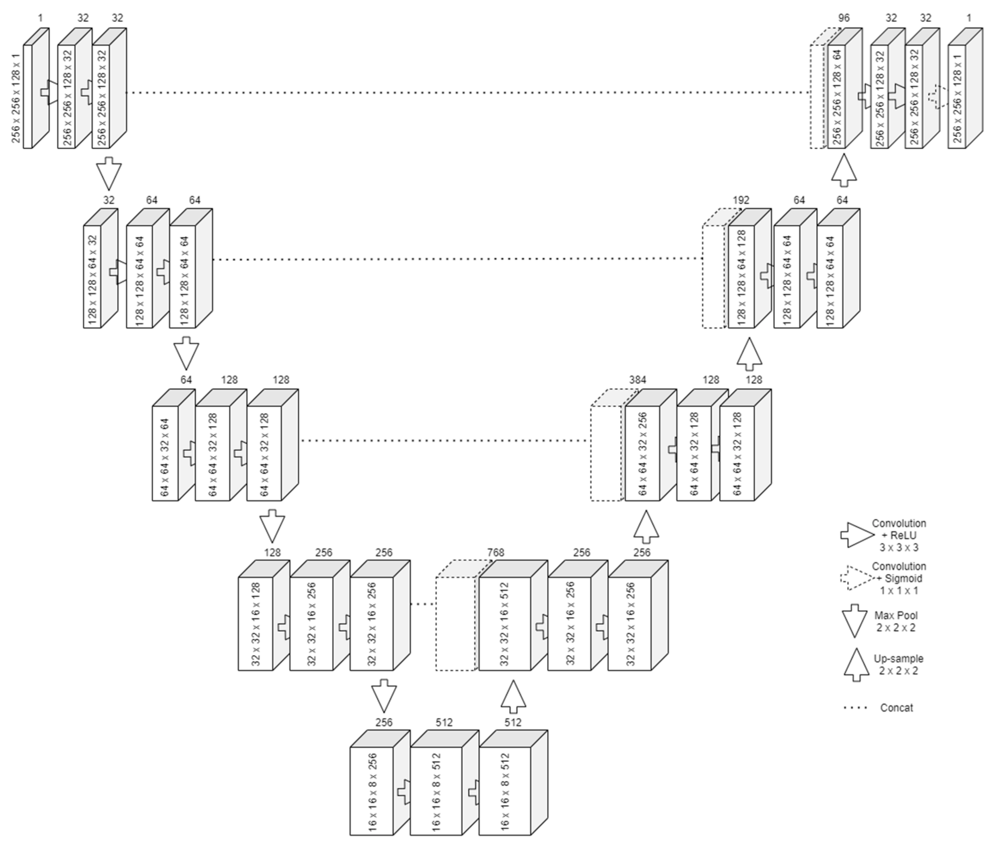
The design of the U-Net follows two important steps, similar to an autoencoder network. The first one is contraction, in which successive rounds of two convolutions and a max pooling to reduce the output size by half are applied on the input, as presented in Figure 1. For each round, the number of filters for the convolution is doubled. The bottom layer will have the most feature maps but will also be the smallest in size. Its purpose is to learn an encoded representation of what it needs to be segmented. The convolution with 3 × 3 × 3 kernels means that one pixel from all the borders will be lost. To alleviate this problem, padding was employed.
The second one is expansion. Starting from the bottom layer, successive rounds of upsampling, concatenate, and two convolutions (also with padding) are applied. The upsampling resizes the feature vector. Along with the information concatenated from the same-size input of the contraction, the two convolutions can reconstruct the image in its original size. Transposed convolution can be used as an operation instead of upsampling. However, this leads to an increased number of parameters to train.
After the last expansion, another convolution is applied with the number of kernels equal to the number of features to extract. Since centerline extraction aims for binary segmentation, only one last kernel with a sigmoid activation function was required.
The loss function is chosen such that the segmentation behaves similarly to a pixel-wise classification function.
3.2. Resize or Patches
The limited amount of the memory of the GPU puts one in the impossibility of feeding an entire CT volume to a neural network. In 2D images, memory is not a problem, even when working with large batches. In 3D, the equivalent would be as if feeding more than 500 images at once in a network.
Our first approach was to resize the volumes (and the ground truth) to a volume that would be small enough to fit in the video RAM but large enough not to lose the details needed for segmentation. The first drawback was that the volumes from the benchmark did not come in a standard size. The X- and Y-axis were always of size 512, but the Z-axis ranged from 272 to 388. This meant that the aspect ratio after any resize to a fixed value would not be constant. Another important loss would be the impossibility to have augmentation under the given circumstances since even the 90-degree rotations would cause big ratio changes. The second drawback of this method was the loss of precision when upscaling. Extracting the centerline would imply getting as good a precision as possible since the vessel fitting algorithms that take as input a centerline depend on this accuracy. Upscaling precision loss can be observed in Figure 2, in which the ground truth centerline is discontinuous and inhomogeneous. Any algorithm without 100% precision would result in something even worse. Training the model using resizing posed problems with the dataset being too small.
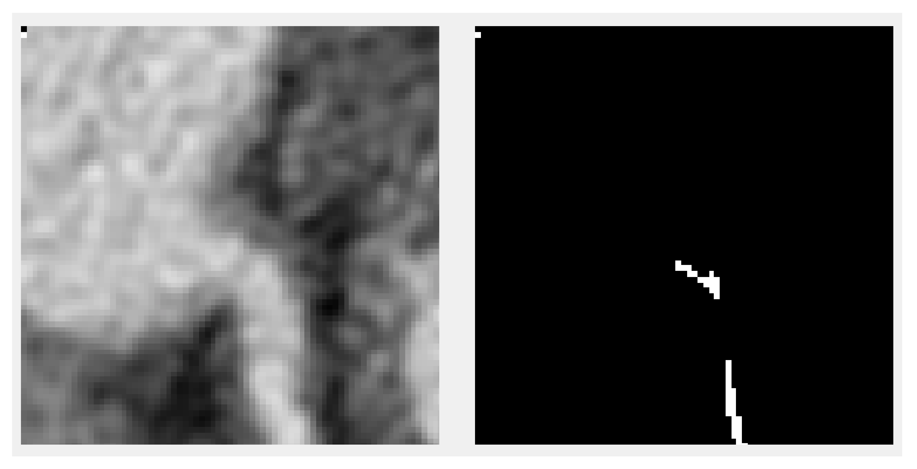
A second approach was proposed to divide the input into smaller patches, cutting only small parts of the volume (and the ground truth) and feeding them to the network. An example slice of a patch together with the associated ground truth is shown in Figure 3. This method does not have any of the downsides of the previous one but introduces a different one—the lack of context. Therefore, a tradeoff is reached between increasing the patch size so that the available contextual information for the model is enough to make a good prediction and the size of the model so that the model is large enough to capture the correlations about where the centerline is positioned and that it should be continuous and also cross the patches.
3.3. Loss Functions
Training neural networks means finding good parameters that make the network approximate a given objective function. For classification tasks, having good accuracy is an objective. For image segmentation tasks, good average pixel-wise classification accuracy could be an objective.
For gradually adjusting weights during the training, a loss function is required. The purpose of the training is to minimize the loss function gradually. A loss function should be chosen to quantify how much and in what direction to adjust the parameters such that on the next iteration, the outputs are closer to the objective.
For image segmentation, numerous loss functions have been proposed in the literature. Some of the existing loss functions for binary segmentation tasks are enumerated here. A new combined loss function that fits the objective of segmenting centerlines is proposed here.
3.3.1. Local Loss
Cross entropy (CE) is defined as follows:
The predicted pixel class is the result of a sigmoid and is interpreted as a probability of belonging to a class. It is then compared with the true class (from the ground truth). Logistic regression is obtained using this loss function.
Weighted cross entropy (WCE) is defined similarly to the cross entropy but adds a coefficient for the positive examples as follows:
It serves in the case of class imbalance in the training dataset. The training might not converge in these cases. The β param controls the expected number of false positives or negatives.
Balanced cross entropy (BCE) is another variation that adds the coefficient for positive examples and the inverted coefficient for negative examples as follows:
Focal loss, introduced in [28] for dense object detection, aims to reduce the problem of huge class imbalances, in which the cross-entropy loss or any of its variations is not enough to achieve stable training. It downweights the “easy” examples to allow training on the rare events, thus the name of focal loss. It is also derived from the cross entropy but adds a focusing parameter γ.
Another variation called class balanced focal loss was introduced in [29].
3.3.2. Global Loss
Dice loss (DL) aims to optimize the F1 score, defined as
which is the harmonic mean between precision and recall. It is considered an overlap measure, as with the Jaccard index. The loss function can be written as
where and .
Balanced dice loss (BDL), also known as Tversky loss, adds a β param to control the expected number of false positives or negatives. It is defined as follows:
3.3.3. Combined Loss Functions
If none of the simple loss functions fits the objective of the neural network, or if the training does not converge, multiple standard loss functions can be combined. An example would be combining a dice coefficient loss with the cross-entropy loss.
To do that, the cross entropy, which outputs individual pixel loss values (called local information), needs to be summed with a loss function on the level of the entire image (called global information). The global loss can be spread to local losses or
the local losses can be averaged.
Distance to the border of the nearest cell (DNC) was introduced for U-Net segmentation in [21]. It combines cross entropy with an averaged distance function for a positive class to the border of two nearest cells. Morphological operations are applied to the image beforehand to compute the border map in the training dataset. The distance to the cells is defined as
and the loss function as
For the U2-Net segmentation [27], a loss function combining Lovász–Softmax (an overlap measure) with the focal loss was used.
3.3.4. Proposed Loss Function
None of the above-mentioned loss functions fit the specifics of our dataset. A function to work with sparsely annotated centerlines is needed, meaning that examples would be contradictory, and at the same time, with a huge class imbalance.
The proposed function is a combination between the focal loss and a simple overlap loss. The overlap loss, defined as follows:
which ensures the stability of the training in spite of the contradicting examples. The focal loss was the only loss with enough power to ignore the huge accuracy of choosing the “easy” example. The focal loss was used with the proposed parameters from the original paper γ = 2 and α = 0.25.
3.4. Generating the Full Output
Since the model takes the input in the shape of patches, it cannot make predictions using a full 3D volume. The simple solution employed was to split the input into blocks of the shape of the patch, pass each of the blocks through the model, and recombine the predictions into a full 3D volume again. If the prediction is qualitative, no artifacts are detected at the border of the combined patches when a segmentation threshold is set.
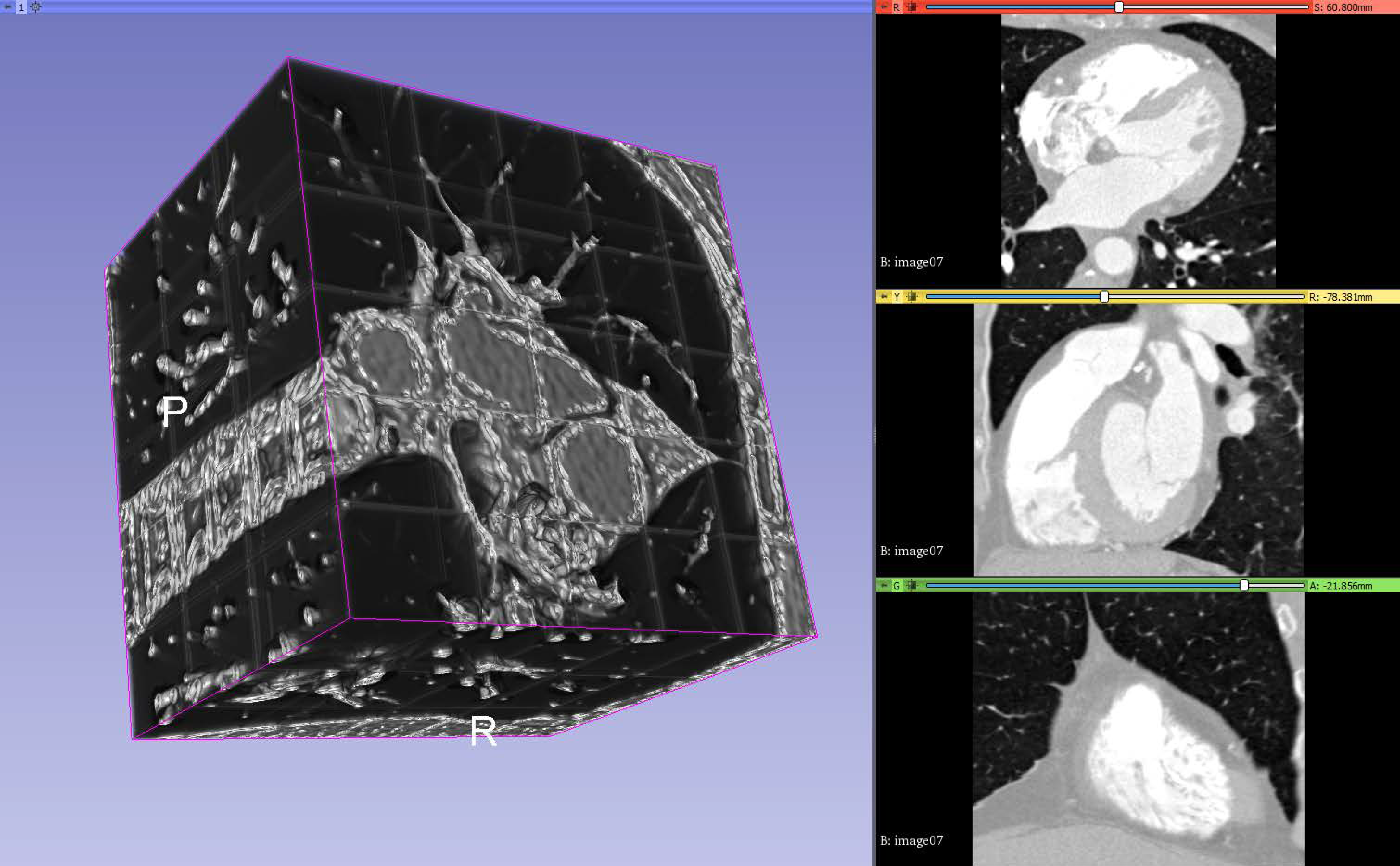
The result is exported as a 3D volume in the same format as the input volumes and generated input masks so that it can be loaded by similar software. One can observe in Figure 4 the output volume composed of patches, in which the threshold is lowered to make it clear where the patches meet.
4. Experimental Results and Discussion
4.1. Coronary Dataset
To test the implementation of the proposed neural network, we chose the dataset from the Rotterdam Coronary Artery Algorithm Evaluation Framework [30]. This is a public benchmark to evaluate algorithms for the task of centerline extraction from CCTA data. The training dataset is publicly available, but nonanonymous registering is required. A standardized quantitative method for evaluating the centerline extraction algorithms is also provided [31].
The dataset is split into a training set and a testing set. The training set consists of 8 volumetric images and the test set consists of 24 volumetric images. All the images have four target vessel descriptions with each containing four reference points (described later). The training set images additionally contain the ground truth in the form of a reference file for the target vessels. This makes it challenging for supervised learning algorithms since many of the vessels are not reported as part of the ground truth. The size and resolution for each training volume are described in Table 1.
The images are packed in two files. One is a “.mhd” ASCII human-readable header file, which describes volume dimensions (e.g., 512 × 512 × 304), the offset, and element spacing (voxel size in real world). The other is a “.raw” file, which contains the voxel (volume pixel) intensities, expressed in Hounsfield units (HU), following the formula intensity = HU + 1024, with a voxel value of zero corresponding to −1024 HU. The format is Insight Toolkit (ITK) compatible.
The ground truth reference files contain a list of the points that are on the centerline of the vessel. The points are described as x,y,z real-world coordinates, the radius of the vessel at that point, and interobserver variability at that position.
There are three categories for extraction: fully automated, minimal user interaction, and interactive extraction [32].
For the fully automated method, two points of reference are provided—one inside the distal part of the vessel, which uniquely identifies the vessel to be tracked, and one at a short distance to the starting point of the centerline.
For the minimal user interaction, only one point is allowed but can be chosen from more options, which include the two points described before, a starting point of a centerline, an endpoint of a centerline, and a user-defined point. The first four points are provided with the downloadable data. A vessel tree can be obtained if one starts from the starting point of the centerline. If that is the case, other reference points can be used.
For the interactive extraction, any given number of reference points can be used, even user-defined points by manual clicking.
4.2. Visualization
A 3D slicer (available from [33]) is a free and open source software platform useful for three-dimensional visualization useful for image-guided therapy (IGT), image processing with registration and interactive segmentation, and medical image informatics. It receives funding support from national health institutes and development support from a large worldwide community of developers with the code available on GitHub (available from [34]). It is directed by National Alliance for Medical Image Computing (NA-MIC), the Neuroimage Analysis Center (NAC), the National Center for Image-Guided Therapy (NCIGT), etc.
The code compiles cross-platform and it is extensible via plug-ins for different algorithms and applications. It supports python scripting for the customization of the look and workflow.
It supports loading DICOM file format for different types of images such as CT, MRI, nuclear medicine, and microscopy. For usage, it contains functionality supported through modules for different organs and contains a bidirectional interface for integration with medical devices.
A 3D Slicer works with scenes, which are a list of elements to be loaded such as images, volumes, models, transforms, fiducial markers. Element extensions include: vtk (Visualization ToolKit), nrrd (Nearly Raw Raster Data), png (Portable Network Graphics), along with the scene file, which is a mrml (Medical Reality Modeling Language); they are archived into a mrb file (Medical Reality Bundle).
Additionally, 3D Slicer provides an out-of-the-box module called volume rendering, used for visually inspect the input volumes, input masks, and output predictions by overlapping them in a 3D space. It provides presets for easy rendering from volumetric images when trying to catch different aspects of the investigation. A “Shift” control allows the user to tamper with the thresholding for rendering features.
4.3. Experimental Setup
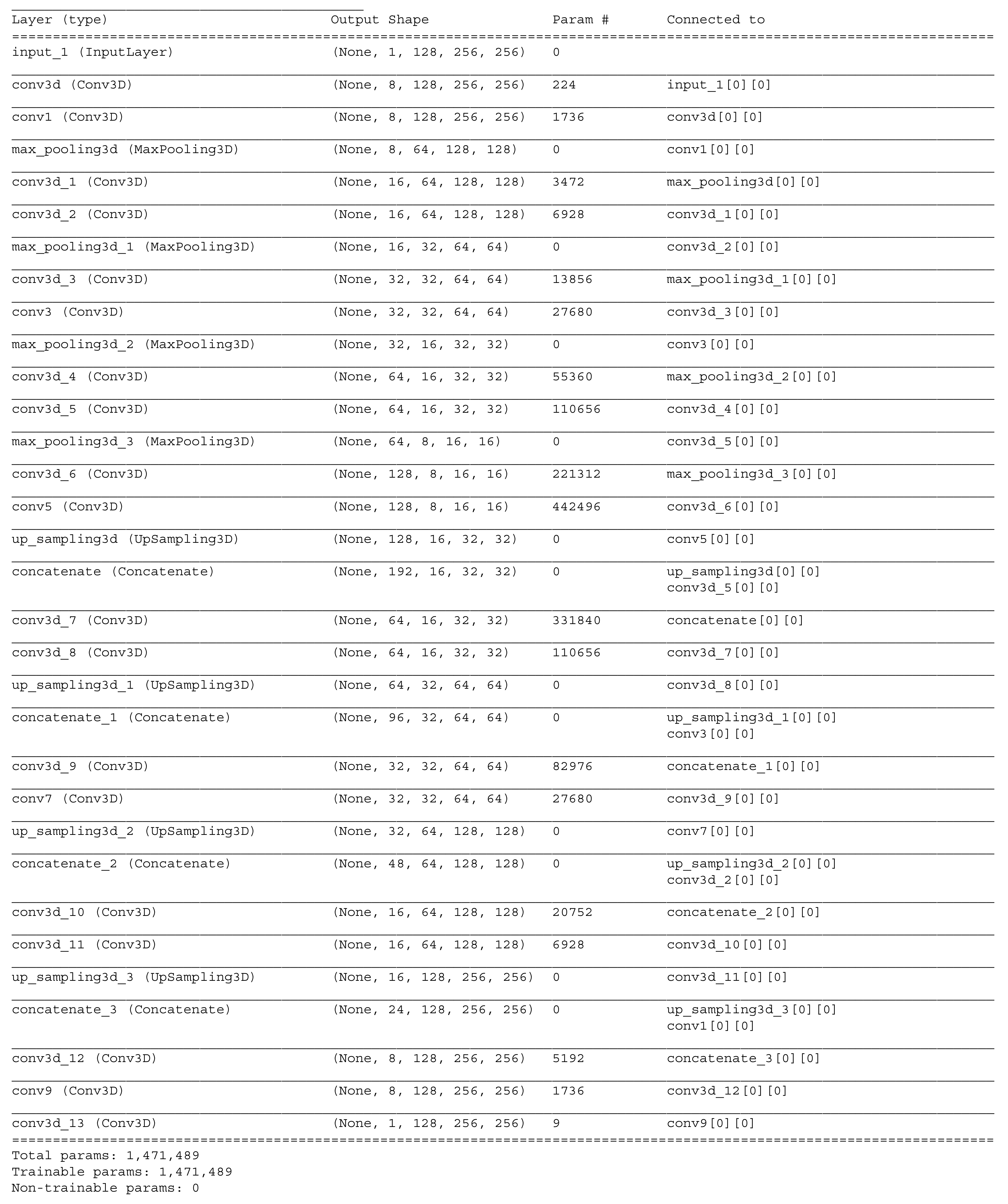
The algorithm was implemented in python using Tensoflow with Keras. The full source code is publicly available at [35]. The provided source code contains the dataset converter and the segmentation algorithm in the form of Python files with executable cells. An example network layout is available in Figure A4. For loading the dataset, we used the SimpleITK python library, and for thinning the obtained centerlines, the skimage package was utilized.
The eight-input volumes with ground truth were split into a training set of seven and a validation set with the remaining volume, leaving one volume out; therefore, the holdout validation was employed. While the number is small, using augmented patches helps reduce the problem of a really small dataset.
The models were trained and tested on an NVIDIA GeForce GTX 1060 with 6GB VRAM. Training required around 8 h on the formerly mentioned video card. The predicting processing time for a patch size input varies between 400 ms and 600 ms, depending on the patch size and model size. For a full volume, this time is multiplied by the number of patches inside a volume. At around 80 patches and 500 ms per patch, the full output is computed in around 40 s. Stitching and postprocessing for saving are negligible in time. The training time makes hyperparameter tuning a strenuous operation, and better configurations can be found by integrating the algorithm into automated design space exploration frameworks. The parameter search space must be more rigidly defined, and the proposed parameters here are a good start.
Following the format of the reference file, we have created a tool to generate a volumetric mask for each input image of the training set, which serves as the ground truth in the supervised learning algorithm. The tool can be parametrized to specify the width in voxels of the centerline. Instead of having a single voxel for one reference point, a cube of a given size is generated, with the center voxel overlapping the centerline. This was found useful in combating the huge class imbalance when working with a single-voxel-wide centerline. The tool outputs the mask in the same format as the input images, with the exception that it can compress the raw data, which is useful when the mask is very sparse. The network will learn centerlines that are thicker than one voxel. A new step of morphological thinning (as described in [36]) must be applied to convert the output of the network into thin centerlines. The overlap and the accuracy are presented with respect to the wide centerlines, not the thinned ones.
4.4. Training the Network
The training of the proposed U-NET architecture was performed with different configurations for the following parameters:
- Input patch size;
- Layer reduction;
- Batch size;
- Feeding or not the network patches with no single voxel of ground truth.
The hard constraint put on the parameters is given by the limited amount of VRAM of the video card. As an example constraint, if the input path size was increased, the batch size or the number of convolutional kernels in the layers needs to be reduced.
The input patch size is described in voxel dimensions as an (X, Y, Z) pair. The tested patch sizes were 128 × 128 × 96, 128 × 128 × 128, 256 × 256 × 128, 320 × 320 × 64, and 384 × 384 × 48.
The layer reduction is the divisor of the number of convolution kernels (the number of output filters in the convolution) for each convolutional layer. Batch size is the number of input volumes fed to the network before backpropagating the error.
When the ground truth is very sparsely distributed along the volume, many of the patches will not have any parts of the segmentation. As measured by experiment, this tends to make the network fall into a local optimum and to always say that there is never anything to segment in the input volume. To prevent this, for patches of a smaller size, the network is fed only inputs that contain at least one segmented ground truth voxel.
A difficult challenge in biomedical image segmentation is the small number of images available for training neural networks. A way to overcome this problem is to use augmentation.
The Batchgenerators framework [37] was used because it provided a wide range of transforms and included spatial augmentation suitable for the 3D input data. The framework allows single or multithreaded computation of the augmented data. An alternative framework that uses the GPU to compute some of the transformations faster is available in [27].
The following spatial transformations were used: random cropping, elastic deformations, rotation on all axes, scaling, and mirroring on all axes. The following color transformations were added: brightness transformation, gamma transformation, and reverse gamma transformation. Noise transformations were also utilized, including Gaussian noise and Gaussian blur. All the transformations are applied with a probability per input sample.
Only the spatial transformations are applied, with the same parameters, to the ground truth. This is conducted in order to keep the annotation in sync with the input volume. Without augmentations, the dataset was too small for the training to converge.
An alternative to the data augmentation presented above will be the use of synthetic data generated using generative adversarial neural networks (GANs), which were applied for medical imaging with success in increasing the accuracy for liver lesion classification [38].
4.5. Results
The classical notation of epoch, in which epoch means one pass over the entire training dataset, will no longer apply when working with randomly cut patches. The term epoch is defined here by multiplying the number of volumes in the training set with the largest input volume size divided on each axis with the corresponding patch size, with the result divided by the batch size. As an example, for a patch size 256 × 256 × 128, a maximum size of an input volume of 512 × 512 × 388, and a batch size of 2, the number of input patches considered to be an epoch is 7 × (512/256) × (512/256) × (388/128)/2 = 7 × 2 × 2 × 3/2 = 42. This formula was used as a rough approximation of feeding the entire volumes once through the network. Due to this definition, the results are reported for different epochs given various input patch sizes. For the training dataset, the values for one epoch are computed as the average across all the input patches. For the validation dataset, the values for one epoch are computed by assembling the whole volume from the output patches and comparing it with the whole ground truth.
The overlap and accuracy measures on the validation data are presented in Table 2. Overlap is defined as the percentage of voxels correctly detected as part of the centerline (analogous to recall), with Equation (11). Accuracy is defined as the percentage of voxels segmented as in the ground truth.
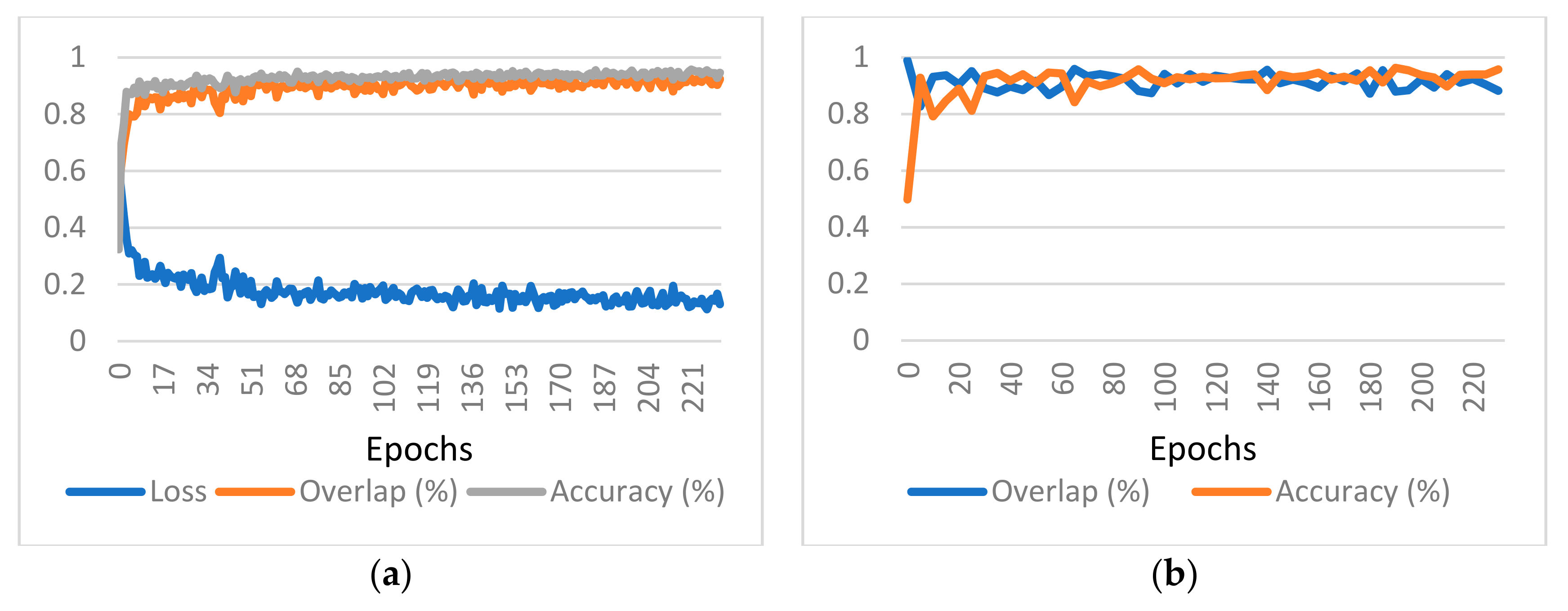
Since the ground truth is presented as sparse centerlines, meaning that only a subset of the coronary vessel tree is annotated, the results cannot be presented using the F1 score or Jaccard index. The number of “false positives” detected by the network will skew the results heavily. Instead, the results are presented in the form of a pair of binary accuracy and overlap (inspired by the results published in [17]). The graphs provided also include the value of the loss function to demonstrate that the learning converges, as depicted in Figure 5 for one of the considered cases. Charts presenting the training and validation evolution for the other configurations can be found in Appendix A.
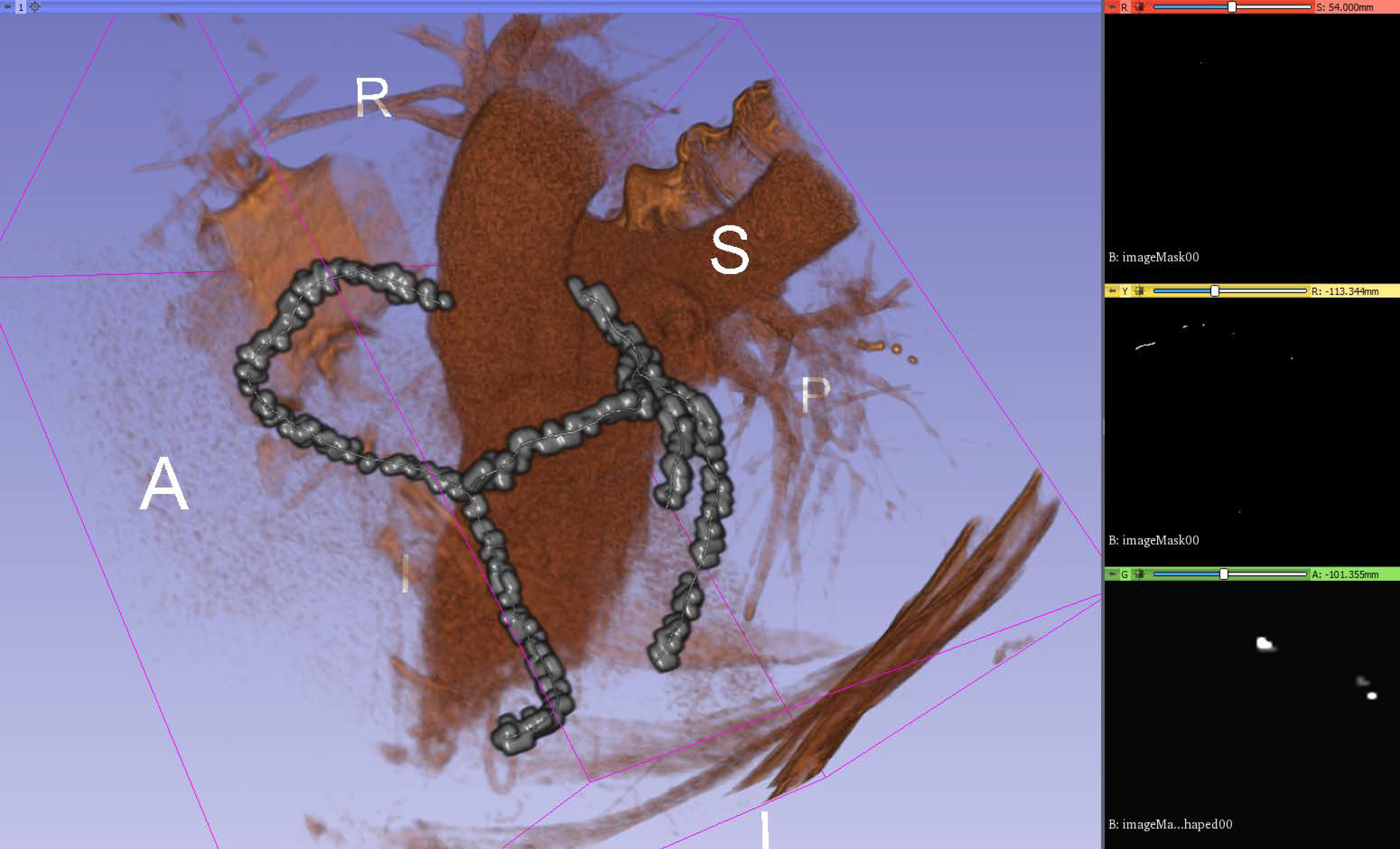
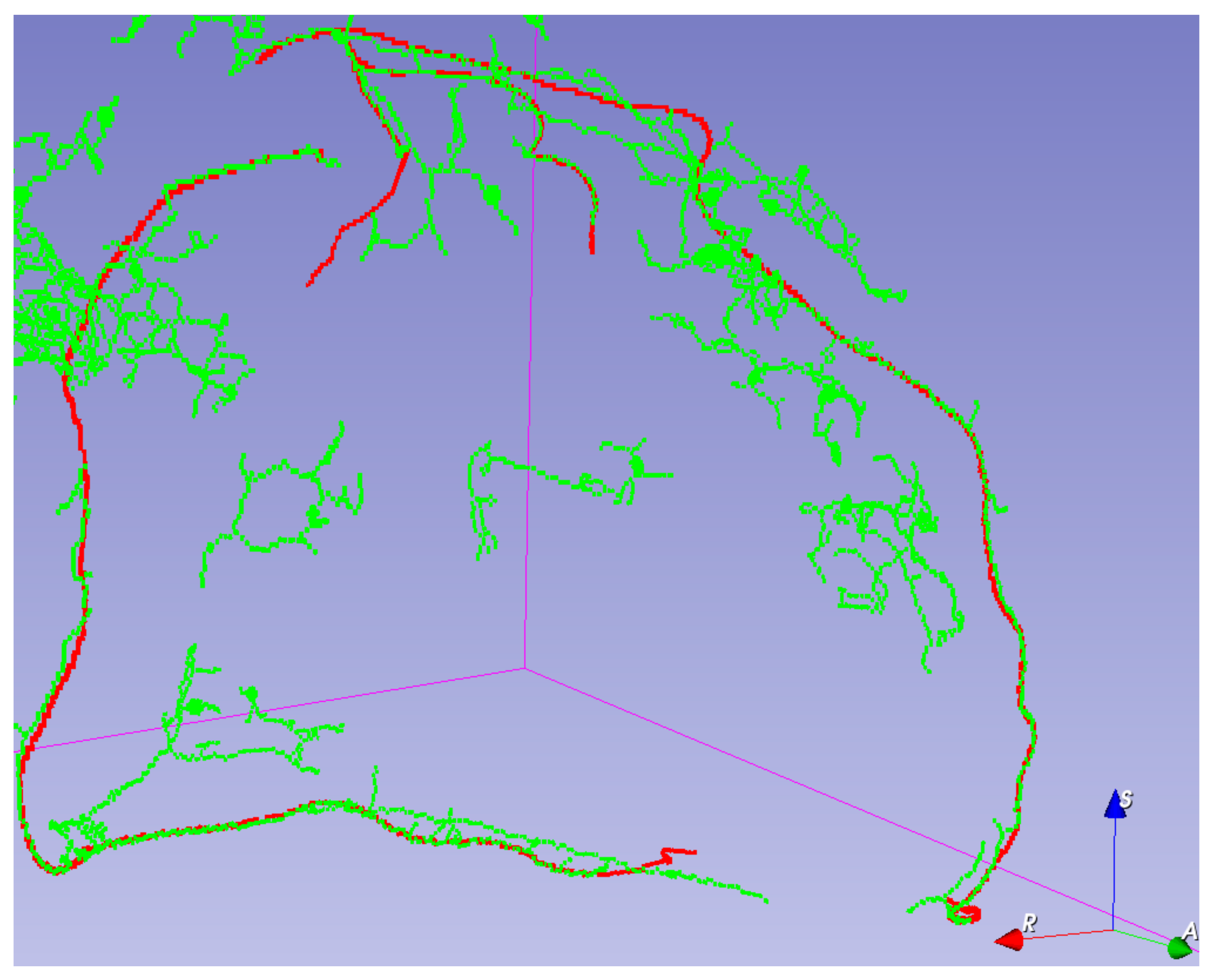
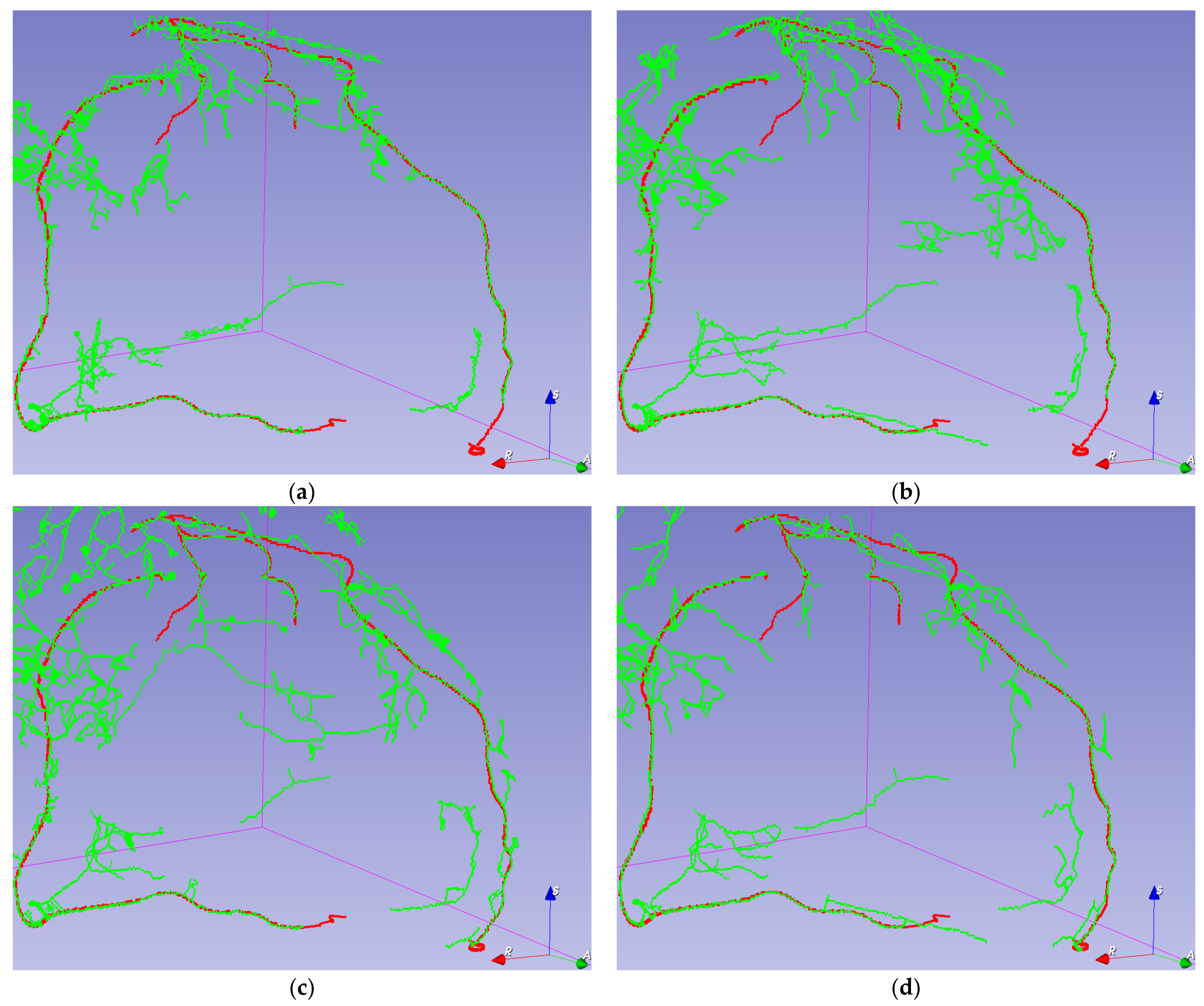
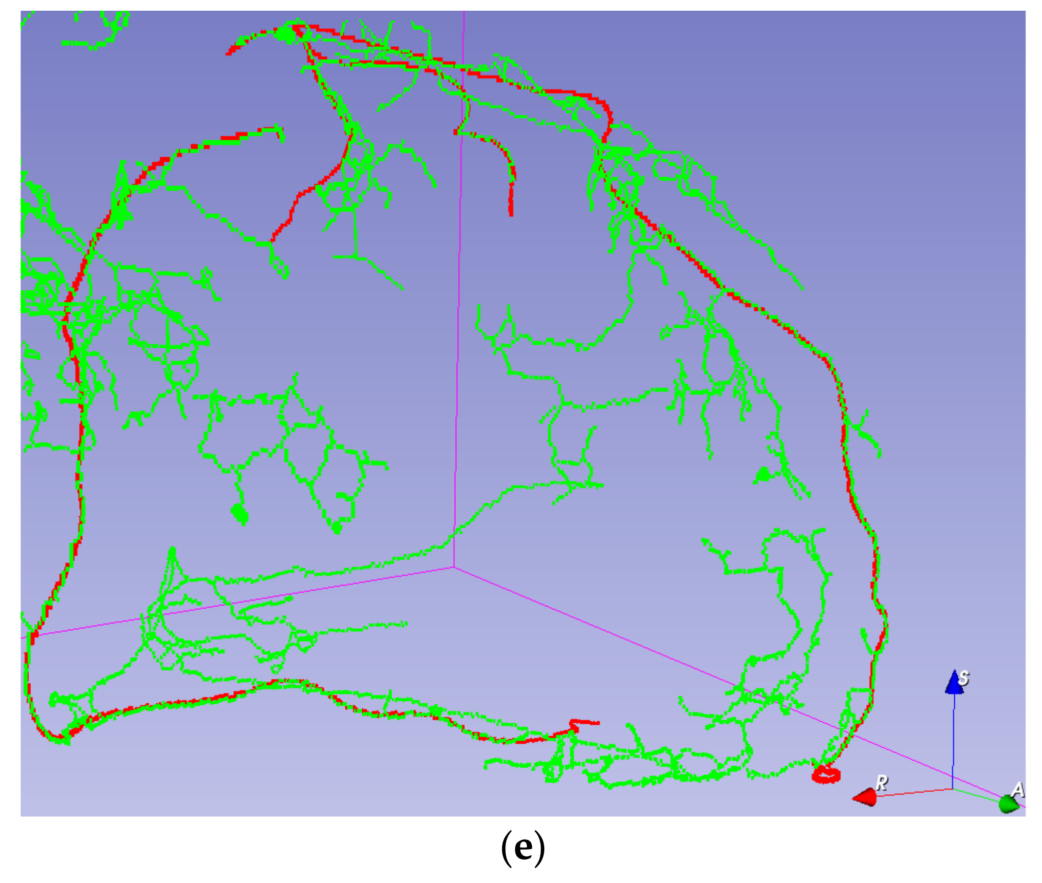
Visual validation for the output volumes is provided, as shown in Figure 6. The ground truth centerline is depicted in red. The segmentation (after thinning) is seen in green, making it easier to check that the segmentation follows the centerline. Visual validation for other training configurations can be found in Figure A3.
5. Discussion
As the patch size increases, the clutter created by smaller vessels decreases. This can be explained by the fact that patches without any ground truth are not avoided since the probability of a long run of them is small. The network better learns to discern when the centerline feels relevant. However, this comes with the cost of also partly losing some of the overlap, but this effect could also be explained by losing the homogeneity of size for the Z dimension.
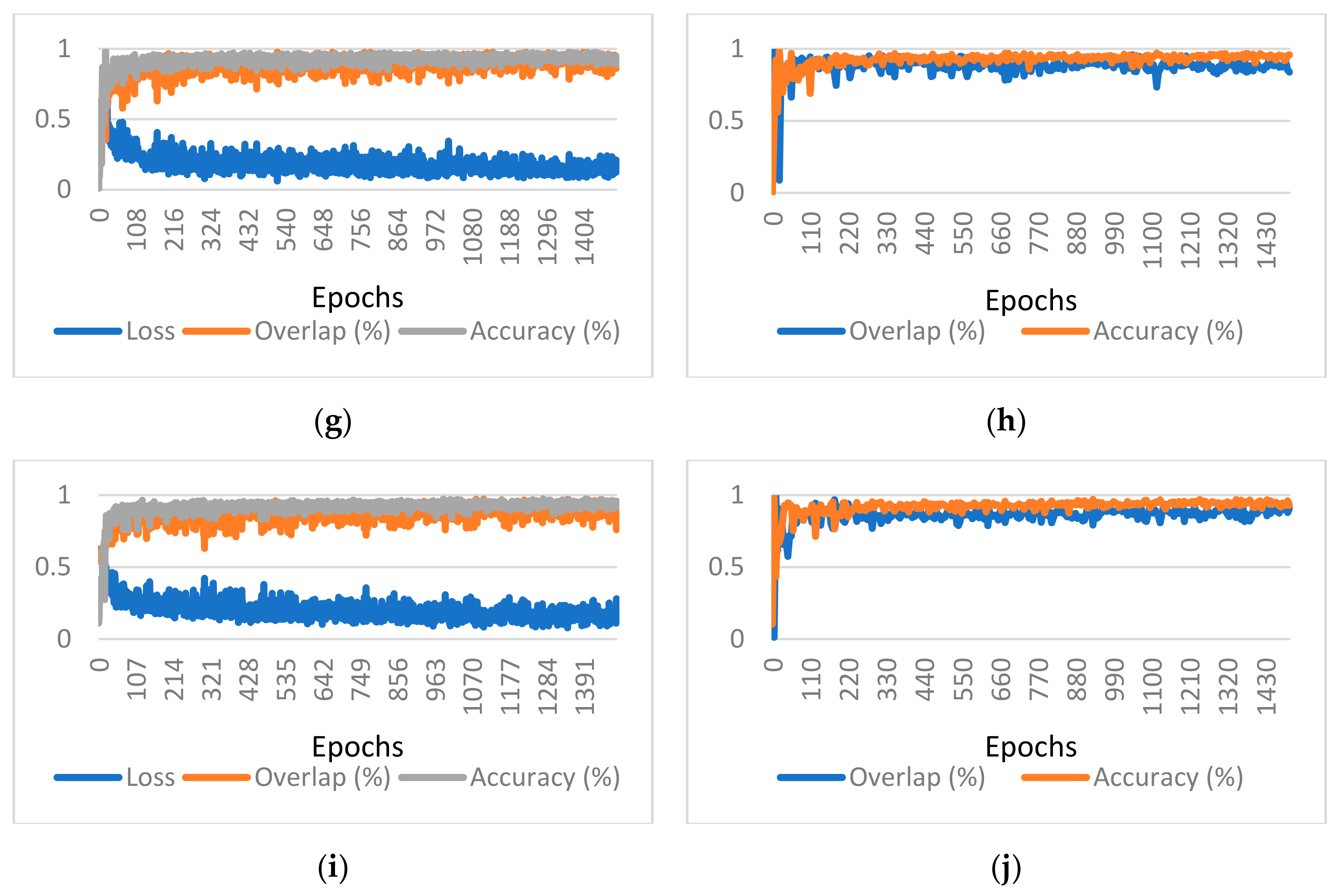
A strong correlation between the patch size and the variance of the training overlap, accuracy, and loss can be observed. This is explained by the smaller number of training examples in an epoch and a greater distortion in the training examples due to augmenting.
It is visible that, as the patch size increases, the number of visual artifacts decreases. We assume that this is due to the network having more contexts to discern which vessels are relevant. Unfortunately, due to constraints on the model size, adding more kernels for bigger patch sizes was not an option.
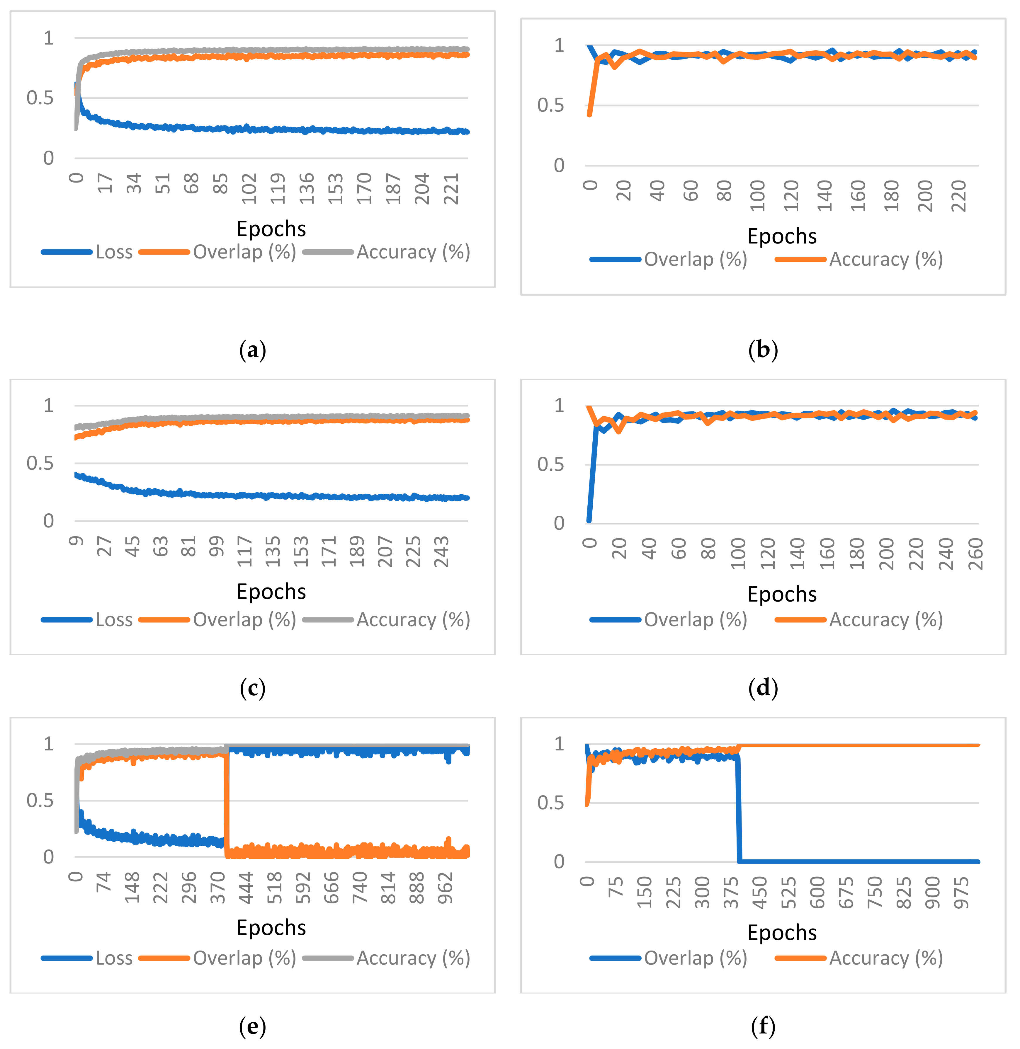
In the case of patch size 256 × 256 × 128, batch size 1, reduction 2, on epoch 393, the randomness in patch selection made the model fall into a local minimum of favoring the accuracy too much. In Figure A1, a huge drop in the overlap and a huge rise in the loss value can be detected. The accuracy jumps to almost 100% due to the class imbalance.
Centerline detection seems to be challenging in very low contrast vessels having fuzzy walls.
6. Conclusions
We have provided an open source (available at [39]) implementation of a 3D U-Net, suitable for segmenting the coronary artery centerline. We have built upon a 2D U-Net-base implementation network, originally designed for retina vessel segmentation, and developed a 3D version capable of segmenting with voxel precision. We have conceived a novel loss function designed to combat two simultaneous problems, usually related to volumetric medical segmentation: huge class imbalance and sparse annotation. Without this loss function, the convergence of the model was not guaranteed even with using augmented inputs. We have built a customizable tool to generate annotated ground truth for the Rotterdam Coronary Artery Centerline Extraction from reference files. We have integrated a 3D augmentation algorithm [37] with the dataset to combat the problem of very few training examples. Without integrating one, the model would not generalize the centerline extraction. We have demonstrated that the training convergence using a second loss function starting with a network pretrained with another loss function. Without the pretraining, training directly with the second loss function would not converge.
As for future improvements, the existing algorithm could benefit from using transfer learning, which was previously applied for U-Net architectures in [40], or for medical image classification models [41]. Even if the training dataset is small for coronary artery centerlines, one can use other segmentation tasks to pretrain the model. Using deconvolution layers instead of upsampling layers in the proposed U-Net architecture may improve the pixel-wise accuracy of the segmentation. The results can be perfected by incorporating a wider training set with data from multiple benchmarks in the same way as in [14,16,17].
Cardiovascular diseases (CVDs), classified as a group of disorders, are the number one cause of death globally [42]. Automated extraction of information about the coronary artery is one step in the computer-aided diagnosis of CVDs. Based on the extracted centerlines, other methods can be employed for visualizations, artery segmentation, plaque detection, and stenosis evaluation. The proposed method can help in improving the visualization, detection, and segmentation of various features such as soft plaque or calcified plaque if included in a stenosis score processing pipeline.
Author Contributions
Conceptualization, A.D., V.O. and R.B.; methodology, A.D. and V.O.; software, A.D.; validation, A.D.; formal analysis, A.D.; investigation, A.D.; resources, A.D.; data curation, A.D.; writing—original draft preparation, A.D.; writing—review and editing, A.D.; visualization, A.D.; su-pervision, R.B. All authors have read and agreed to the published version of the manuscript.
Funding
This research received no external funding.
Institutional Review Board Statement
Not applicable.
Informed Consent Statement
Not applicable.
Data Availability Statement
The data presented in this study are available on request from the corresponding author. The data are not publicly available due to data confidentiality.
Conflicts of Interest
The authors declare no conflict of interest.
Appendix A. Graph Results for Considered Hyperparameters
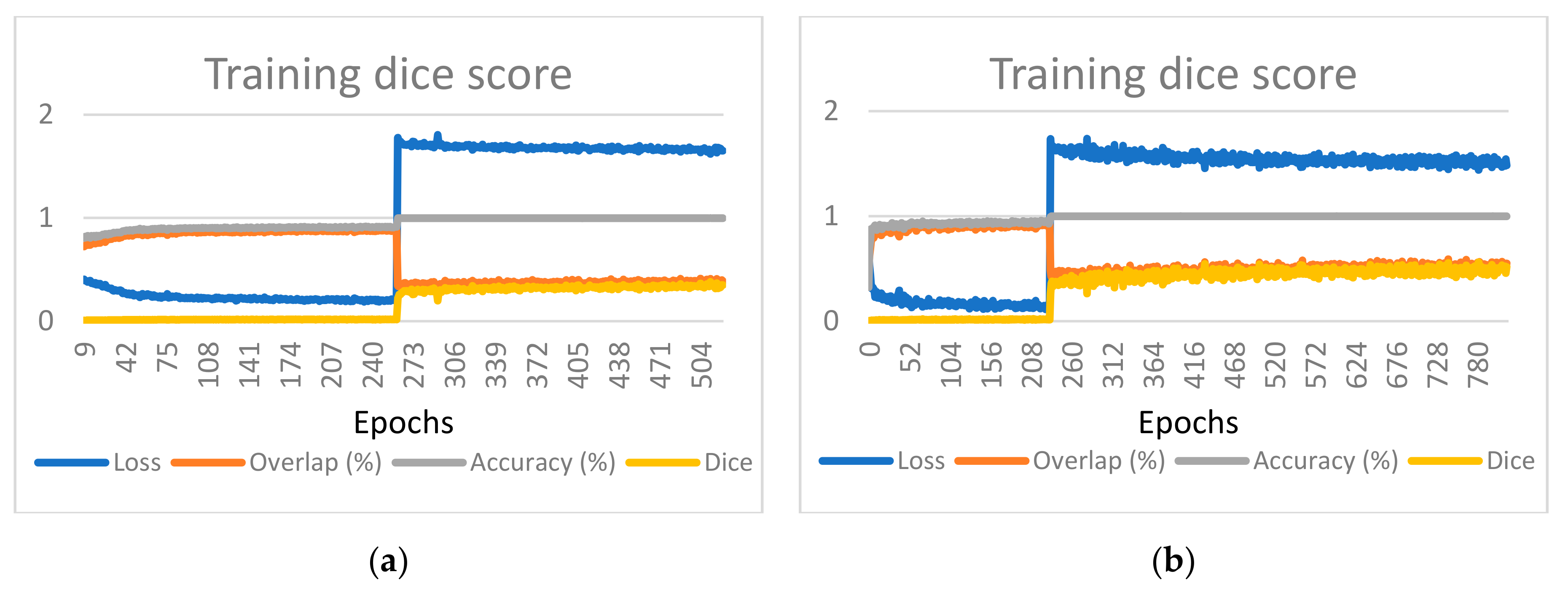
Figure A1.
Graphs of the evaluation metrics for different parameter configurations for training and validation, respectively, (a,b) 128 × 128 × 96, batch size 1, reduction 1, only patches with ground truth; (c,d) 128 × 128 × 128, batch size 2, reduction 2, only patches with ground truth; (e,f) 256 × 256 × 128, batch size 1, reduction 2; (g,h) 320 × 320 × 64, batch size 1, reduction 4; and (i,j) 384 × 384 × 48, batch size 1, reduction 4.


Starting from a randomly initialized model, with a dice coefficient loss function, which optimizes the tradeoff between precision and recall, the training converges quickly to predicting nothing. This happens because of two reasons—the huge class imbalance and the sparse annotation of the centerlines, where the model receives mixed signals about what represents a centerline and what does not. A different validation approach was used by starting to train the model with the proposed loss function, and when the model is sufficiently trained, switching to dice loss. The training now converges, and an increase in the dice coefficient can be seen in Figure A2. Of course, this is not necessarily the objective since the data are sparsely annotated, but this is another confirmation that the results are on the right track. We further present the results in terms of dice coefficient after switching the training objective. Similar behavior is observed for the patch size 128 × 128 × 128 or for the patch size 256 × 256 × 128 (Figure A2).
Figure A2.
Loss function switch for (a) patch size 128 × 128 × 128 and (b) Patch size 256 × 256 × 128.
Figure A2.
Loss function switch for (a) patch size 128 × 128 × 128 and (b) Patch size 256 × 256 × 128.

The loss function switch determines a rapid growth of the loss, marking a clear transition. The accuracy goes to almost 100% because the model is now inclined to almost predict nothing. However, unlike the previous instability case, in which the overlap fell to zero, it can now be inferred that the overlap jumps to around 40% and starts to slowly increase with each epoch. For the first part of the training, the dice coefficient was close to zero since we had a lot of “false positives” with respect to the annotated ground truth. The second part of the training leads to an increase in the dice coefficient, which is expected because the loss function optimizes for that. Since the dice coefficient closely matches the overlap, it can be assumed that the model does not predict too much outside of the high confidence zone. A simple dice function would output a number between −1 and 1. We added 1 to the result to avoid displaying negative values.
Appendix B. Visual Validation for Other Training Configurations
Figure A3.
Visual validation for different parameter configurations. The ground truth centerline is depicted in red. The segmentation (after thinning) is seen in green for (a) 128 × 128 × 96, batch size 1, reduction 1, only patches with ground truth; (b) 128 × 128 × 128, batch size 2, reduction 2, only patches with ground truth; (c) 256 × 256 × 128, batch size 1, reduction 2; (d) 320 × 320 × 64, batch size 1, reduction 4; and (e) 384 × 384 × 48, batch size 1, reduction 4.


Appendix C. Input Size 256 × 256 × 128, Model Reduction 4
Figure A4.
Neural network model summary for Input Size 256 × 256 × 128, Model Reduction 4.

References
- Galal, H.; Rashid, T.; Alghonaimy, W.; Kamal, D. Detection of positively remodeled coronary artery lesions by multislice CT and its impact on cardiovascular future events. Egypt Heart J. 2019, 71, 26. [Google Scholar] [CrossRef] [Green Version]
- Pantos, I.; Katritsis, D. Fractional Flow Reserve Derived from Coronary Imaging and Computational Fluid Dynamics. Interv. Cardiol. Rev. 2014, 9, 145. [Google Scholar] [CrossRef] [Green Version]
- Zhao, Y.; Ping, J.; Yu, X.; Wu, R.; Sun, C.; Zhang, M. Fractional flow reserve-based 4D hemodynamic simulation of time-resolved blood flow in left anterior descending coronary artery. Clin. Biomech. 2019, 70, 164–169. [Google Scholar] [CrossRef] [PubMed]
- Williams, L.H.; Drew, T. What do we know about volumetric medical image interpretation? A review of the basic science and medical image perception literatures. Cogn. Res. 2019, 4, 21. [Google Scholar] [CrossRef] [PubMed] [Green Version]
- Zhao, F.; Chen, Y.; Hou, Y.; He, X. Segmentation of blood vessels using rule-based and machine-learning-based methods: A review. Multimed. Syst. 2019, 25, 109–118. [Google Scholar] [CrossRef]
- Chen, X.; Fu, Y.; Lin, J.; Ji, Y.; Fang, Y.; Wu, J. Coronary Artery Disease Detection by Machine Learning with Coronary Bifurcation Features. Appl. Sci. 2020, 10, 7656. [Google Scholar] [CrossRef]
- Danilov, A.; Pryamonosov, R.; Yurova, A. Image Segmentation for Cardiovascular Biomedical Applications at Different Scales. Computation 2016, 4, 35. [Google Scholar] [CrossRef] [Green Version]
- Bates, R.; Irving, B.; Markelc, B.; Kaeppler, J.; Muschel, R.; Grau, V.; Schnabel, J.A. Extracting 3D Vascular Structures from Microscopy Images using Convolutional Recurrent Networks. arXiv 2017, arXiv:1705.09597. [Google Scholar]
- Han, D.; Shim, H.; Jeon, B.; Jang, Y.; Hong, Y.; Jung, S.; Ha, S.; Chang, H.-J. Automatic Coronary Artery Segmentation Using Active Search for Branches and Seemingly Disconnected Vessel Segments from Coronary CT Angiography. PLoS ONE 2016, 11, e0156837. [Google Scholar] [CrossRef] [PubMed]
- Liu, L.; Xu, J.; Liu, Z. Automatic segmentation of coronary lumen based on minimum path and image fusion from cardiac computed tomography images. Clust. Comput 2019, 22, 1559–1568. [Google Scholar] [CrossRef]
- Kong, B.; Wang, X.; Bai, J.; Lu, Y.; Gao, F.; Cao, K.; Xia, J.; Song, Q.; Yin, Y. Learning tree-structured representation for 3D coronary artery segmentation. Comput. Med. Imaging Graph. 2020, 80, 101688. [Google Scholar] [CrossRef]
- Lv, T.; Yang, G.; Zhang, Y.; Yang, J.; Chen, Y.; Shu, H.; Luo, L. Vessel segmentation using centerline constrained level set method. Multimed Tools Appl. 2019, 78, 17051–17075. [Google Scholar] [CrossRef]
- Gao, Z.; Liu, X.; Qi, S.; Wu, W.; Hau, W.K.; Zhang, H. Automatic segmentation of coronary tree in CT angiography images. Int. J. Adapt. Control. Signal. Process. 2019, 33, 1239–1247. [Google Scholar] [CrossRef]
- Sheng, X.; Fan, T.; Jin, X.; Jin, J.; Chen, Z.; Zheng, G.; Lu, M.; Zhu, Z. Extraction Method of Coronary Artery Blood Vessel Centerline in CT Coronary Angiography. IEEE Access 2019, 7, 170690–170702. [Google Scholar] [CrossRef]
- Cui, H.; Xia, Y. Automatic Coronary Centerline Extraction Using Gradient Vector Flow Field and Fast Marching Method From CT Images. IEEE Access 2018, 6, 41816–41826. [Google Scholar] [CrossRef]
- Guo, Z.; Bai, J.; Lu, Y.; Wang, X.; Cao, K.; Song, Q.; Sonka, M.; Yin, Y. DeepCenterline: A Multi-task Fully Convolutional Network for Centerline Extraction. In Information Processing in Medical Imaging; Chung, A.C.S., Gee, J.C., Yushkevich, P.A., Bao, S., Eds.; Lecture Notes in Computer Science; Springer International Publishing: Cham, Switzerland, 2019; Volume 11492, pp. 441–453. ISBN 978-3-030-20350-4. [Google Scholar]
- Wolterink, J.M.; van Hamersvelt, R.W.; Viergever, M.A.; Leiner, T.; Išgum, I. Coronary artery centerline extraction in cardiac CT angiography using a CNN-based orientation classifier. Med. Image Anal. 2019, 51, 46–60. [Google Scholar] [CrossRef] [PubMed] [Green Version]
- Sainath, T.N.; Vinyals, O.; Senior, A.; Sak, H. Convolutional, Long Short-Term Memory, fully connected Deep Neural Networks. In Proceedings of the 2015 IEEE International Conference on Acoustics, Speech and Signal Processing (ICASSP); IEEE: South Brisbane, Australia, 2015; pp. 4580–4584. [Google Scholar] [CrossRef]
- Salahuddin, Z.; Lenga, M.; Nickisch, H. Multi-Resolution 3D Convolutional Neural Networks for Automatic Coronary Centerline Extraction in Cardiac CT Angiography Scans. arXiv 2020, arXiv:2010.00925. [Google Scholar]
- He, J.; Pan, C.; Yang, C.; Zhang, M.; Wang, Y.; Zhou, X.; Yu, Y. Learning Hybrid Representations for Automatic 3D Vessel Centerline Extraction. In Medical Image Computing and Computer Assisted Intervention—MICCAI 2020; Martel, A.L., Abolmaesumi, P., Stoyanov, D., Mateus, D., Zuluaga, M.A., Zhou, S.K., Racoceanu, D., Joskowicz, L., Eds.; Lecture Notes in Computer Science; Springer International Publishing: Cham, Switzerland, 2020; Volume 12266, pp. 24–34. ISBN 978-3-030-59724-5. [Google Scholar]
- Ronneberger, O.; Fischer, P.; Brox, T. U-Net: Convolutional Networks for Biomedical Image Segmentation. In Medical Image Computing and Computer-Assisted Intervention—MICCAI 2015; Navab, N., Hornegger, J., Wells, W.M., Frangi, A.F., Eds.; Lecture Notes in Computer Science; Springer International Publishing: Cham, Switzerland, 2015; Volume 9351, pp. 234–241. ISBN 978-3-319-24573-7. [Google Scholar]
- Irving, B.; Hutton, C.; Dennis, A.; Vikal, S.; Mavar, M.; Kelly, M.; Brady, J.M. Deep Quantitative Liver Segmentation and Vessel Exclusion to Assist in Liver Assessment. In Medical Image Understanding and Analysis; Valdés Hernández, M., González-Castro, V., Eds.; Communications in Computer and Information Science; Springer International Publishing: Cham, Switzerland, 2017; Volume 723, pp. 663–673. ISBN 978-3-319-60963-8. [Google Scholar]
- Jin, Q.; Meng, Z.; Pham, T.D.; Chen, Q.; Wei, L.; Su, R. DUNet: A deformable network for retinal vessel segmentation. Knowl. Based Syst. 2019, 178, 149–162. [Google Scholar] [CrossRef] [Green Version]
- Zhuang, J. LadderNet: Multi-path networks based on U-Net for medical image segmentation. arXiv 2019, arXiv:1810.07810. [Google Scholar]
- Guo, C.; Szemenyei, M.; Yi, Y.; Wang, W.; Chen, B.; Fan, C. SA-UNet: Spatial Attention U-Net for Retinal Vessel Segmentation. arXiv 2020, arXiv:2004.03696. [Google Scholar]
- Çiçek, Ö.; Abdulkadir, A.; Lienkamp, S.S.; Brox, T.; Ronneberger, O. 3D U-Net: Learning Dense Volumetric Segmentation from Sparse Annotation. arXiv 2016, arXiv:1606.06650. [Google Scholar]
- Huang, C.; Han, H.; Yao, Q.; Zhu, S.; Zhou, S.K. 3D U2-Net: A 3D Universal U-Net for Multi-domain Medical Image Segmentation. In Proceedings of the Medical Image Computing and Computer Assisted Intervention—MICCAI 2019; Shen, D., Liu, T., Peters, T.M., Staib, L.H., Essert, C., Zhou, S., Yap, P.-T., Khan, A., Eds.; Springer International Publishing: Cham, Switzerland, 2019; Volume 11765, pp. 291–299. [Google Scholar] [CrossRef] [Green Version]
- Lin, T.-Y.; Goyal, P.; Girshick, R.; He, K.; Dollár, P. Focal Loss for Dense Object Detection. arXiv 2018, arXiv:1708.02002. [Google Scholar]
- Cui, Y.; Jia, M.; Lin, T.-Y.; Song, Y.; Belongie, S. Class-Balanced Loss Based on Effective Number of Samples. arXiv 2019, arXiv:1901.05555. [Google Scholar]
- Rotterdam Coronary Artery Algorithm Evaluation Framework. Available online: http://coronary.bigr.nl/centerlines/ (accessed on 11 January 2020).
- Schaap, M.; Metz, C.T.; van Walsum, T.; van der Giessen, A.G.; Weustink, A.C.; Mollet, N.R.; Bauer, C.; Bogunović, H.; Castro, C.; Deng, X. Standardized evaluation methodology and reference database for evaluating coronary artery centerline extraction algorithms. Med. Image Anal. 2009, 13, 701–714. [Google Scholar] [CrossRef] [Green Version]
- Rotterdam Coronary Artery Challenge Categories. Available online: http://coronary.bigr.nl/centerlines/about.php (accessed on 11 January 2020).
- 3D Slicer. Available online: https://www.slicer.org/ (accessed on 11 January 2020).
- GitHub Slicer. Available online: https://github.com/Slicer/Slicer (accessed on 11 January 2020).
- Alexandru Dorobanțiu—GitHub. Available online: https://github.com/AlexDorobantiu (accessed on 11 May 2019).
- Jonker, P.P. Morphological Operations on 3D and 4D Images: From Shape Primitive Detection to Skeletonization. In Discrete Geometry for Computer Imagery; Borgefors, G., Nyström, I., di Baja, G.S., Eds.; Lecture Notes in Computer Science; Springer: Berlin/Heidelberg, Germany, 2000; Volume 1953, pp. 371–391. ISBN 978-3-540-41396-7. [Google Scholar]
- MIC-DKFZ/batchgenerators. Available online: https://github.com/MIC-DKFZ/batchgenerators (accessed on 29 August 2020).
- Frid-Adar, M.; Diamant, I.; Klang, E.; Amitai, M.; Goldberger, J.; Greenspan, H. GAN-based synthetic medical image augmentation for increased CNN performance in liver lesion classification. Neurocomputing 2018, 321, 321–331. [Google Scholar] [CrossRef] [Green Version]
- AlexDorobantiu/CoronaryCenterlineUnet. Available online: https://github.com/AlexDorobantiu/CoronaryCenterlineUnet (accessed on 29 August 2020).
- Iglovikov, V.; Shvets, A. TernausNet: U-Net with VGG11 Encoder Pre-Trained on ImageNet for Image Segmentation. arXiv 2018, arXiv:1801.05746. [Google Scholar]
- Manzo, M.; Pellino, S. Bucket of Deep Transfer Learning Features and Classification Models for Melanoma Detection. J. Imaging 2020, 6, 129. [Google Scholar] [CrossRef]
- WHO—Cardiovascular diseases (CVDs) Fact Sheet. Available online: https://www.who.int/news-room/fact-sheets/detail/cardiovascular-diseases-(cvds) (accessed on 24 September 2020).
Figure 1.
The proposed 3D U-Net architecture.

Figure 2.
Downscaled and upscaled centerline ground truth (80 × 80 × 64) plotted in 3D to highlight the difficulty of using it for training.
Figure 2.
Downscaled and upscaled centerline ground truth (80 × 80 × 64) plotted in 3D to highlight the difficulty of using it for training.

Figure 3.
A 2D slice of an augmented patch with ground truth next to it.

Figure 4.
Output volume composed of patches with visible stitching.

Figure 5.
Patch size 256 × 256 × 128: (a) training only with ground truth patches and (b) validation.
Figure 5.
Patch size 256 × 256 × 128: (a) training only with ground truth patches and (b) validation.

Figure 6.
Patch size 256 × 256 × 128; a 3D Slicer rendering of ground truth (red) and centerline segmentation (green).
Figure 6.
Patch size 256 × 256 × 128; a 3D Slicer rendering of ground truth (red) and centerline segmentation (green).


Table 1.
The size and resolution of each CTA volume from the training dataset.
| CTA | Size (Voxels) | Resolution (mm3) |
|---|---|---|
| dataset00 | 512 × 512 × 272 | 0.363 × 0.363 × 0.4 |
| dataset01 | 512 × 512 × 338 | 0.363 × 0.363 × 0.4 |
| dataset02 | 512 × 512 × 288 | 0.334 × 0.334 × 0.4 |
| dataset03 | 512 × 512 × 276 | 0.371 × 0.371 × 0.4 |
| dataset04 | 512 × 512 × 274 | 0.316 × 0.316 × 0.4 |
| dataset05 | 512 × 512 × 274 | 0.322 × 0.322 × 0.4 |
| dataset06 | 512 × 512 × 268 | 0.320 × 0.320 × 0.4 |
| dataset07 | 512 × 512 × 304 | 0.287 × 0.287 × 0.4 |
Table 2.
The overlap and accuracy results for the selected hyperparameters.
| Patch Size | Batch Size | Model Reduction | Patches with Ground Truth Only | Epoch | Overlap | Accuracy |
|---|---|---|---|---|---|---|
| 128 × 128 × 96 | 1 | 1 | true | 231 | 0.934 | 0.921 |
| 128 × 128 × 128 | 2 | 2 | true | 260 | 0.895 | 0.940 |
| 256 × 256 × 128 | 1 | 2 | true | 232 | 0.917 | 0.943 |
| 256 × 256 × 128 | 1 | 2 | false | 392 | 0.944 | 0.911 |
| 320 × 320 × 64 | 1 | 4 | false | 1250 | 0.883 | 0.953 |
| 384 × 384 × 48 | 1 | 4 | false | 1500 | 0.910 | 0.928 |
Publisher’s Note: MDPI stays neutral with regard to jurisdictional claims in published maps and institutional affiliations. |
© 2021 by the authors. Licensee MDPI, Basel, Switzerland. This article is an open access article distributed under the terms and conditions of the Creative Commons Attribution (CC BY) license (https://creativecommons.org/licenses/by/4.0/).
Share and Cite
MDPI and ACS Style
Dorobanțiu, A.; Ogrean, V.; Brad, R. Coronary Centerline Extraction from CCTA Using 3D-UNet. Future Internet 2021, 13, 101. https://0-doi-org.brum.beds.ac.uk/10.3390/fi13040101
AMA Style
Dorobanțiu A, Ogrean V, Brad R. Coronary Centerline Extraction from CCTA Using 3D-UNet. Future Internet. 2021; 13(4):101. https://0-doi-org.brum.beds.ac.uk/10.3390/fi13040101
Chicago/Turabian StyleDorobanțiu, Alexandru, Valentin Ogrean, and Remus Brad. 2021. "Coronary Centerline Extraction from CCTA Using 3D-UNet" Future Internet 13, no. 4: 101. https://0-doi-org.brum.beds.ac.uk/10.3390/fi13040101
Note that from the first issue of 2016, this journal uses article numbers instead of page numbers. See further details here.