Exploiting Machine Learning for Improving In-Memory Execution of Data-Intensive Workflows on Parallel Machines

Abstract

Workflows are largely used to orchestrate complex sets of operations required to handle and process huge amounts of data. Parallel processing is often vital to reduce execution time when complex data-intensive workflows must be run efficiently, and at the same time, in-memory processing can bring important benefits to accelerate execution. However, optimization techniques are necessary to fully exploit in-memory processing, avoiding performance drops due to memory saturation events. This paper proposed a novel solution, called the Intelligent In-memory Workflow Manager (IIWM), for optimizing the in-memory execution of data-intensive workflows on parallel machines. IIWM is based on two complementary strategies: (1) a machine learning strategy for predicting the memory occupancy and execution time of workflow tasks; (2) a scheduling strategy that allocates tasks to a computing node, taking into account the (predicted) memory occupancy and execution time of each task and the memory available on that node. The effectiveness of the machine learning-based predictor and the scheduling strategy were demonstrated experimentally using as a testbed, Spark, a high-performance Big Data processing framework that exploits in-memory computing to speed up the execution of large-scale applications. In particular, two synthetic workflows were prepared for testing the robustness of the IIWM in scenarios characterized by a high level of parallelism and a limited amount of memory reserved for execution. Furthermore, a real data analysis workflow was used as a case study, for better assessing the benefits of the proposed approach. Thanks to high accuracy in predicting resources used at runtime, the IIWM was able to avoid disk writes caused by memory saturation, outperforming a traditional strategy in which only dependencies among tasks are taken into account. Specifically, the IIWM achieved up to a $31\%$ and a $40\%$ reduction of makespan and a performance improvement up to $1.45\times$ and $1.66\times$ on the synthetic workflows and the real case study, respectively.

1. Introduction

A data-intensive workflow is a process that usually involves a set of computational steps implementing complex scientific functions, such as data acquisition, transformation, analysis, storage, and visualization [1]. Parallelism can be achieved by concurrently executing independent tasks by trying to make use of all computing nodes, even if, in many cases, it is necessary to execute multiple tasks on the same computing node [2]. For example, this occurs when the number of tasks is greater than the number of available nodes or because multiple tasks use a dataset located on the same node. These scenarios are prone to memory saturation, and moving data to disk may result in higher execution times, which leads to the need for a scheduling strategy able to cope with this issue [3,4].

In most cases, distributed processing systems use a priori policies for handling task execution and data management. For example, in the MapReduce programming model used by Hadoop, mappers write intermediate results after each computation, so performing disk-based processing with partial use of memory [5] through the exploitation of the Hadoop Distributed File System (HDFS). On the other hand, Apache Spark (https://spark.apache.org/, accessed on 3 May 2021), which is a state-of-the-art data analysis framework for large-scale data processing exploiting in-memory computing, relies on a Directed Acyclic Graph (DAG) paradigm and is based on: (i) an abstraction for data collections that enables parallel execution and fault-tolerance, named Resilient Distributed Datasets (RDDs) [6]; (ii) a DAG engine, which manages the execution of jobs, stages, and tasks. Besides, it provides different storage levels for data caching and persistence, while performing in-memory computing with partial use of the disk. The Spark in-memory approach is generally more efficient, but a time overhead may be caused by spilling data from memory to disk when memory usage exceeds a given threshold [7]. This overhead can be significantly reduced if the memory occupancy of a task is known in advance, to avoid running in parallel two or more tasks that cumulatively exceed the available memory, thus causing data spilling. For this reason, memory is considered a key factor for the performance and stability of Spark jobs, and Out-of-Memory (OOM) errors are often hard to fix. Recent efforts have been oriented towards developing prediction models for the performance estimation of Big Data applications, although most of the approaches rely on analytical models, and only a few recent studies have investigated the use of supervised machine learning models [8,9,10].

In this work, we propose a system, named the Intelligent In-memory Workflow Manager (IIWM), specially designed for improving application performance through intelligent usage of memory resources. This is done by identifying clusters of tasks that can be executed in parallel on the same node, optimizing in-memory processing, so avoiding the use of disk storage.Given a data-intensive workflow, the IIWM exploits a regression model for estimating the amount of memory occupied by each workflow task and its execution time. This model is trained on a log of past executed workflows, represented in a transactional way through a set of relevant features that characterize the considered workflow, such as:

• Workflow structure, in terms of tasks and data dependencies.
• Input format, such as the number of rows, dimensionality, and all other features required to describe the complexity of input data.
• The types of tasks, i.e., the computation performed by a given node of the workflow. For example, in the case of data analysis workflows, we can distinguish among supervised learning, unsupervised learning, and association rule discovery tasks, as well as between learning and prediction tasks.

Predictions made for a given computing node are applicable to all computing nodes of the same type (i.e., having the same architecture, processor type, operating system, memory resources), which makes the proposed approach effectively usable on large-scale homogeneous HPC systems composed of many identical servers. Given a data-intensive workflow, the IIWM exploits the estimates coming from the machine learning model for producing a scheduling plan aimed at reducing (and, in most cases, avoiding) main memory saturation events, which may happen when multiple tasks are executed concurrently on the same computing node. This leads to the improvement of application performance, as swapping or spilling to disk caused by main memory saturation may result in significant time overhead, which can be particularly costly when running workflows involving very large datasets and/or complex tasks.

The IIWM was experimentally evaluated using as a testbed, Spark, which is expected to become the most adopted Big Data engine in the next few years [11]. In particular, we assessed the benefits coming from the use of the IIWM by executing two synthetic workflows specially generated for investigating specific scenarios related to the presence of a high level of parallelism and a limited amount of memory reserved for execution. The effectiveness of the proposed approach was further confirmed through the execution of a real data mining workflow as a case study. We carried out an in-depth comparison between the IIWM and a traditional blind scheduling strategy, which only considers workflow dependencies for the parallel execution of tasks. The proposed approach was shown to be the most suitable solution in all evaluated scenarios, outperforming the blind strategy thanks to high accuracy in predicting resources used at runtime, which leads to the minimization of disk writes caused by memory saturation.

The rest of the paper is organized as follows. Section 2 discusses related work. Section 3 describes the proposed system. Section 4 presents and discusses the experimental results. Section 5 concludes the paper.

Problem Statement

The problem addressed in this study consists of the optimization of the in-memory execution of data-intensive workflows, evaluated in terms of makespan (i.e., the total time required to process all given tasks) and application performance. The main reason behind the drop in performance in such workflows is related to the necessity of swapping/spilling data to disk when memory saturation events occur. To cope with this issue, we proposed an effective way of scheduling a workflow that minimizes the probability of memory saturation, while maximizing in-memory computing and, thus, performance.

A workflow $\mathcal{W}$ can be represented using a DAG, described by a set of tasks $\mathcal{T}=\{t_1,t_2,\dots ,t_n\}$ (i.e., vertices) and dependencies among them $\mathcal{A}\subseteq (\mathcal{T}\times \mathcal{T})=\{a_1,\dots ,a_m\}$: $a_i=(t_i,t_j),t_i\in \mathcal{T},t_j\in \mathcal{T}$ (i.e., directed edges). Specifically, data dependencies (i.e., all the input data of a task have already been made available) have to be considered rather than control dependencies (i.e., all predecessors of a task must be terminated before it can be executed), as we refer to data-intensive workflows [12].

Formally, given a set of q computing resources $R=\{r_1,\dots ,r_q\}$, workflow scheduling can be defined as the mapping $\mathcal{T}\to R$ from each task $t\in \mathcal{T}$ to a resource $r\in R$, so as to meet a set of specified constraints, which influence the choice of an appropriate scheduling strategy [13]. Workflow scheduling techniques are often aimed at optimizing several factors, including makespan and overall cost that in turn depend on data transfer and compute cost [14]. In this study, a multi-objective optimization was applied, jointly minimizing execution time and memory saturation. This is achieved by using a scheduling strategy that exploits a regression model aimed at predicting the behavior of a given workflow, in terms of resource demand and execution time (see Section 3). For the reader’s convenience,

Table 1. Meaning of the main symbols.

Symbol	Meaning
$\mathcal{T}=\{t_1,t_2,\dots ,t_n\}$	Set of tasks.
$\mathcal{A}\subseteq (\mathcal{T}\times \mathcal{T})=\{a_1,\dots ,a_m\}$	Dependencies. $a_i=(t_i,t_j),t_i\in \mathcal{T},t_j\in \mathcal{T}$.
$d_t$	Description of the dataset processed by task t.
$\mathcal{W}=(\mathcal{T},\mathcal{A})$	Workflow.
${\mathcal{N}}^{in}\left(t\right)=\{t^{\prime }\in \mathcal{T}\mid (t^{\prime },t)\in \mathcal{A}\}$	In-neighborhood of task t.
${\mathcal{N}}^{out}\left(t\right)=\{t^{\prime }\in \mathcal{T}\mid (t,t^{\prime })\in \mathcal{A}\}$	Out-neighborhood of task t.
$\mathcal{M}$	Regression prediction model.
$\mathcal{S}=\langle s_1,\dots ,s_k\rangle$	List of stages. $s_i\subseteq \mathcal{T}\mid (t_x\Vert t_y)\forall t_x,t_y\in s_i$.
C	Maximum amount of memory available for a computing node.
$C_s=C-{\displaystyle \sum _{t\in s}}\mathcal{M}.predict\_mem(t,d_t)$	Residual capacity of a stage s.

shows the meaning of the main symbols used in the paper.

2. Related Work

Recent studies have shown the effectiveness of machine learning-based prediction modeling in supporting code optimization, parallelism mapping, task scheduling, and processor resource allocation [10]. Moreover, predicting running times and memory footprint is important for estimating the cost of execution and better managing resources at runtime [11]. For instance, in-memory data processing frameworks like Spark can benefit from the informed co-location of tasks [10]. In fact, if too many applications or tasks are assigned to a computing node, such that the memory used on the host exceeds the available one, memory paging to disk (i.e., swapping), data spilling to disk in Spark, or OOM errors can occur with consequential drops in performance.

Our work focused on improving the performance of a Spark application using machine learning-based techniques. The challenge is to effectively schedule tasks in a data-intensive workflow for improving resource usage and application performance, by inferring the resource demand of each task, in terms of memory occupancy and time.

State-of-the-art techniques aimed at improving the performance of data-intensive applications can be divided into two main categories: analytical-based and machine learning-based. For each category, the main proposed solutions and their differences with respect to our technique are discussed.

2.1. Analytical-Based

Techniques in this category use information collected at runtime and statistics in order to tune a Spark application, improving its performance as follows:

• Choosing the serialization strategy for caching RDDs in RAM, based on previous statistics collected on different working sets, such as memory footprint, CPU usage, RDDs size, serialization costs, etc. [15,16].
• Dynamically adapting resources to data storage, using a feedback-based mechanism with real-time monitoring of the memory usage of the application [17].
• Scheduling jobs by dynamically adjusting concurrency through a feedback-based strategy. Taking into account memory usage via garbage collection, network I/O, and Spark RDDs lineage information, it is possible to choose the number of tasks to assign to an executor [18,19].

The aforementioned works used different strategies to improve in-memory computing of Spark that exploit static or dynamic techniques able to introduce some information in the choice of configuration parameters. However, no prediction models were employed, and this may lead to unpredicted behaviors. The IIWM, instead, uses a prediction regression model to estimate a set of information about a running Spark application, exploiting it to optimize in-memory execution. Moreover, unlike real-time adapting strategies, which use a feedback-based mechanism by continuously monitoring the execution, the IIWM model is trained offline, achieving fast and accurate predictions while being used for inferring the resource demand of each task in a given workflow.

2.2. Machine Learning-Based

These techniques are based on the development of learning models for predicting performance (mainly memory occupancy and execution time) of a large set of different applications in several scenarios, on the basis of prior knowledge. This enables the adoption of a performance-centric approach [8], based on an informed performance improvement, which can be beneficial for the execution of data-intensive applications, especially in the context of HPC systems.

Several techniques use collaborative filtering to identify how well an application will run on a computing node. For instance, Quasar [8] uses classification techniques based on collaborative filtering to determine the characteristics of the running application in allocating resources and assigning tasks. When submitted, a new application is briefly profiled, and the collected information is combined with the classification engine, based on previous workloads, to support a greedy scheduling policy that improves throughput. The application is monitored throughout the execution to adjust resource allocation and assignment if required, using a single model for the estimation. Adapting this technique to Spark can help to assign tasks to computing nodes within the memory constraints and avoid exceeding the capacity, thus causing the spilling of data to disk. Another approach based on collaborative filtering was proposed by Llull et al. [9]. In this case, the task co-location problem is modeled as a cooperative game, and a game-theoretic framework, namely Cooper, is proposed for improving resource usage. The algorithm builds pairwise coalitions as stable marriages to assign an additional task to a host based on its available memory, and the Spark default scheduler is adopted to assign tasks. In particular, a predictor receives performance information collected offline and estimates which co-runner is better, in order to find stable co-locations.

Moving away from collaborative filtering, Marco et al. [10] presented a mixture-of-experts approach to model the memory behavior of Spark applications. It is based on a set of memory models (i.e., linear regression, exponential regression, Napierian logarithmic regression) trained on a wide variety of applications. At runtime, an expert selector based on k-nearest neighbor (kNN) is used to choose the model that best describes memory behavior, in order to determine which tasks can be assigned to the same host for improving throughput. The memory models and expert selector are trained offline on different working sets, recording the memory used by a Spark executor through the Linux command “/proc”. Finally, the scheduler uses the selected model to determine how much memory is required for an incoming application, for improving server usage and system throughput.

Similar to machine learning-based techniques, the IIWM exploits a prediction model trained on execution logs of previous workflows; however, it differs in two main novel aspects: (i) the IIWM only uses high-level workflow features, without requiring any runtime information, as done in [8,10], in order to avoid the overhead that could not be negligible for complex applications; (ii) it provides an algorithm for effectively scheduling a workflow in scenarios with limited computing resources.

As far as we know, no similar approaches in the literature can be directly compared to the IIWM in terms of the goals and requirements. In fact, differently from the IIWM, Quasar [8] and Cooper [9] can be seen as resource-efficient cluster management systems, aimed at optimizing QoS constraints and resource usage. With respect to the most related work, presented in [10], the IIWM presents the following differences.

• It focuses on data-intensive workflows, while in [10], general workloads were addressed.
• It uses high-level information for describing an application (e.g., task and dataset features), while in [10], low-level system features were exploited, such as the cache miss rate and the number of blocks sent, collected by running the application on a small portion (100 MB) of the input data.
• It proposes a more general approach, since the approach proposed in [10] is only appliable to applications whose memory usage is a function of the input size.

3. Materials and Methods

The Intelligent In-memory Workflow Manager (IIWM) is based on three main steps:

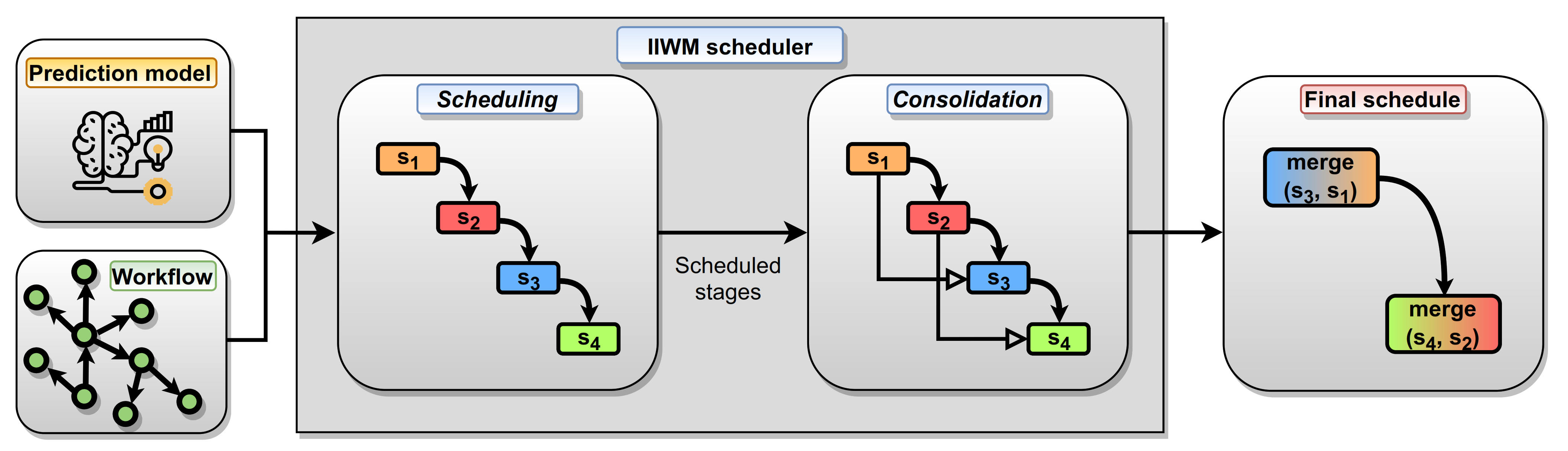
• Execution monitoring and dataset creation: starting from a given set of workflows, a transactional dataset is generated by monitoring the memory usage and execution time of each task, specifying how it is designed and giving concise information about the input.
• Prediction model training: from the transactional dataset of executions, a regression model is trained in order to fit the distribution of memory occupancy and execution time, according to the features that represent the different tasks of a workflow.
• Workflow scheduling: taking into account the predicted memory occupancy, and execution time of each task, provided by the trained model, and the available memory of the computing node, tasks are scheduled using an informed strategy. In this way, a controlled degree of parallelism can be ensured, while minimizing the risk of memory saturation.

In the following sections, a detailed description of each step is provided.

3.1. Execution Monitoring and Dataset Creation

The first step in the IIWM consists of monitoring the execution of different tasks on several input datasets with variable characteristics, in order to build a transactional dataset for training the regression model. The proposed solution was specifically designed for supporting the efficient execution of data analysis tasks, which are used in a wide range of data-intensive workflows. Specifically, it focuses on three classes of data mining tasks: classification tasks for supervised learning, clustering tasks for unsupervised learning, and association rule discovery. Using Spark as a testbed, the following data mining algorithms from the MLlib (https://spark.apache.org/mllib/, accessed on 3 May 2021) library were used: decision tree, naive Bayes, and Support Vector Machines (SVMs) for classification tasks; K-means and Gaussian Mixture Models (GMMs) for clustering tasks; FPGrowth for association rule tasks.

3.1.1. Execution Monitoring within the Spark Unified Memory Model

As far as execution monitoring is concerned, a brief overview of the Spark unified memory model is required. In order to avoid OOM errors, Spark uses up to 90% of the heap memory, which is divided into three categories: reserved memory (300 MB), used to store Spark internal objects; user memory (40% of heap memory), used to store data structures and RDDs computed during transformations and actions; Spark memory (60% of heap memory), divided into execution and storage. The former refers to that used for computation during shuffle, join, sort, and aggregation processes, while the latter is used for caching RDDs. It is worth noting that, when no execution memory is used, storage can acquire all the available memory and vice versa. However, storage may not evict execution due to complexities in implementation, while stored data blocks are evicted from main memory according to a Least Recently Used (LRU) strategy.

The occupancy of storage memory relies on the persistence operations performed natively by the algorithms.

Table 2. Examples of persist calls in MLlib algorithms.

MLlib Algorithm	Persist Call
K-Means	//Compute squared norms and cache them norms.cache()
Decision Tree	//Cache input RDD for speedup during multiple passes BaggedPoint.convertToBaggedRDD(treeInput,…).cache()
GMM	instances.cache()   …  data.map(_.asBreeze).cache()
FPGrowth	items.cache()
SVM	IstanceBlock.blokifyWithMaxMemUsage(…).cache()

reports some examples of data caching implemented in the aforementioned MLlib algorithms. In particular, the cache() call corresponds to persist(StorageLevel.MEMORY_AND_DISK), where MEMORY_AND_DISK is the default storage level used for the recent API based on DataFrames.

According to the Spark unified memory model, the execution monitoring was done via the Spark REST APIs, which expose executor-level performance metrics, collected in a JSON file, including peak occupancy for both execution and storage memory along with execution time.

3.1.2. Dataset Creation

Using the aforementioned Spark APIs, we monitored the execution of several MLlib algorithms on different input datasets, covering the main data mining tasks, i.e., classification, clustering, and association rules. The goal of this process was the creation of a transactional dataset for the regression model training, which contained the following information:

• The description of the task, such as its class (e.g., classification, clustering, etc.), type (fitting or predicting task), and algorithm (e.g., SVM, K-means, etc.).
• The description of the input dataset in terms of the number of rows, columns, categorical columns, and overall dataset size.
• Peak memory usage (both execution and storage) and execution time, which represent the three target variables to be predicted by the regressor. In order to obtain more significant data, the metrics were aggregated on median values by performing ten executions per task.

For the sake of clarity,

Table 3. A sample of the training dataset.

Task Name	Task Type	Task Class	Dataset Rows	Dataset Columns	Categorical Columns	Dataset Size (MB)	Peak Storage Memory (MB)	Peak Execution Memory (MB)	Duration (ms)
GMM	Estimator	Clustering	1,474,971	28	0	87.00	433.37	1413.50	108,204.00
K-Means	Estimator	Clustering	5,000,000	104	0	1239.78	4624.52	4112.00	56,233.50
Decision Tree	Estimator	Classification	9606	1921	0	84.91	730.09	297.90	39,292.00
Naive Bayes	Estimator	Classification	260,924	4	0	13.50	340.92	6982.80	16,531.50
SVM	Estimator	Classification	5,000,000	129	0	1542.58	6199.11	106.60	238,594.50
FPGrowth	Estimator	Association Rules	823,593	180	180	697.00	9493.85	1371.03	96,071.50
GMM	Transformer	Clustering	165,474	14	1	6.37	2.34	1 × 10${}^{-6}$	62.50
K-Means	Transformer	Clustering	4,898,431	42	3	648.89	3.23	1 × 10${}^{-6}$	35.00
Decision Tree	Transformer	Classification	1,959,372	42	4	257.69	3.68	1 × 10${}^{-6}$	65.50
Naive Bayes	Transformer	Classification	347,899	4	0	17.99	4.26	1 × 10${}^{-6}$	92.50
SVM	Transformer	Classification	5,000,000	129	0	1542.58	2.36	1 × 10${}^{-6}$	55.50
FPGrowth	Transformer	Association Rules	136,073	34	34	13.55	1229.95	633.50	52,429.00
…	…	…	…	…	…	…	…	…	…

shows a sample of the dataset described above.

Starting from 20 available datasets, we divided them into two partitions used for training and testing, respectively. Afterwards, an oversampling procedure was performed, aimed at increasing the number of datasets contained in the partitions. Specifically, a naive random sampling approach can lead to unexpected behaviors regarding the convergence of algorithms, thus introducing noise into the transactional dataset used to build the regression model. To cope with this issue, we used the following feature selection strategy:

• For datasets used in classification or regression tasks, we considered only the k highest scoring features based on:

  –

  the analysis of variance (F-value) for integer labels (classification problems);

  –

  the correlation-based univariate linear regression test for real labels (regression problems).

• For clustering datasets, we used a correlation-based test to maintain the k features with the smallest probability to be correlated with the others.
• For association rule discovery datasets, no feature selection is required, as the number of columns refers to the average number of items in the different transactions.

The described procedure was applied separately on the training and test partitions, so as to avoid the introduction of bias into the evaluation process. Specifically, the number of datasets in the training and test partitions was increased from 15 to 260 and from 5 to 86, respectively. Subsequently, we fed these datasets to the MLlib algorithms, obtaining two final transactional datasets of 1309 and 309 monitored executions, used for training and testing the regressor, respectively.

3.2. Prediction Model Training

Once the training and test datasets with memory and time information were built, a regression model could be trained with the goal of estimating peak memory occupancy and turnaround time of a task in a given workflow.

As a preliminary step, we analyzed the correlation between the features of the training data and each target variable, using the Spearman index. We obtained the following positive correlations: a value of $0.30$ between storage memory and the input dataset size, $0.46$ between execution memory and the task class, and $0.21$ between execution time and the number of columns. These results can be seen in detail in Figure 1.

Afterwards, we moved to the training of the regression model. Due to its complexity, the regression problem cannot be faced with a simple linear regressor or its regularized variants (e.g., Ridge, Lasso, or ElasticNet), but a more robust model is necessary. We experimentally evaluated this aspect by testing the forecasting abilities of these linear models, achieving poor results. For this reason, an ensemble learning model was used in order to fit the nonlinear distribution of features. Specifically, the stacking technique (meta learning) [20] was used by developing a two-layer model in which a set of regressors was trained on the input dataset and a decision tree was fit on their predictions. The first layer consisted of three tree-based regressors, able to grasp different aspects of input data: a gradient boosting, an AdaBoost, and an extra trees regressor. The second layer exploits a single decision tree regressor, which predicts the final value starting from the concatenation of the outputs from the first layer. The described ensemble model was set with the hyperparameters shown in

Table 4. Hyperparameters.

Hyperparameter	Value
n_estimators	500
learning_rate	0.01
max_depth	7
loss	least squares

.

Among 20 trained models, initialized with different random states, we selected the best one by maximizing the following objective function:

$$\mathcal{O}={\overline{R}}^2-MAE$$

whose goal is to choose the model that best explains the variance of the data, while minimizing the forecasting error. This function jointly considers the adjusted determination coefficient (${\overline{R}}^2$), which guarantees robustness with respect to the addition of useless variables to the model compared to the classical $R^2$ score, and the Mean Absolute Error (MAE), normalized with respect to the maximum.

The described model was developed in Python3 using the scikit-learn (https://scikit-learn.org/stable/, accessed on 3 May 2021) library and evaluated against the test set of 309 unseen executions obtained as described in Section 3.1.2. Thanks to the combination of different models, the ensemble technique was shown to be very well suited for this task, leading to good robustness against outliers and a high forecasting accuracy, as shown in Figure 2.

These results are detailed in

Table 5. Evaluation metrics on the test set.

	RMSE	MAE	Adjusted ${\mathit{R}}^2$	Pearson Correlation
Storage Memory	$108.23$	$26.66$	$0.96$	$0.98$
Execution Memory	$312.60$	$26.30$	$0.91$	$0.95$
Duration	4443.17	2003.70	$0.95$	$0.98$

, which shows the evaluation metrics for each target variable, including the ${\overline{R}}^2$ score and the Pearson correlation coefficient. In particular, the Mean Absolute Error (MAE) and the Root Mean Square Error (RMSE) for the storage and execution memory represent average errors in megabytes, while for the duration, they represent errors in milliseconds.

3.3. Workflow Scheduling

The prediction model described in Section 3.2 can be exploited to forecast the amount of memory that will be needed to execute a given task on a target computing node and its duration, based on the task features listed in Section 3.1. These predictions are then used within the scheduling strategy described in the following, whose goal is to avoid swapping to disk due to memory saturation in order to improve application performance and makespan through a better use of in-memory computing. The results discussed below refer to a static scheduling problem, as the scheduling plan is generated before the execution. In typical static scheduling, the workflow system has to predict the execution load of each task accurately, using heuristic-based methods [21]. Likewise, in the proposed method, the execution load of each task of a given workflow is predicted by the model trained on past executions. Moreover, we investigated how workflow tasks can be scheduled and run on a single computing node, but this approach can be easily generalized to a multi-node scenario. For example, a data-intensive workflow can be decomposed into multiple sub-workflows to be run on different computing nodes according to their features and data locality. Each sub-workflow is scheduled locally to the assigned node using the proposed strategy.

In the IIWM, we modeled the scheduling problem as an offline Bin Packing (BP). This is a well-known problem, widely used for resource and task management or scheduling, such as load balancing in mobile cloud computing architectures [22], energy-efficient execution of data-intensive applications in clouds [23], DAGs’ real-time scheduling in heterogeneous clusters [24], and task scheduling in multiprocessor environments [25]. Its classical formulation is as follows [26]. Let n be the number of items, $w_j$ the weight of the j-th item, and c the capacity of each bin: the goal is to assign each item to a bin without exceeding the capacity c and minimizing the number of used bins. The problem is $\mathcal{NP}$-complete, and much effort went into finding fast algorithms with near-optimal solutions. We adapted the classical problem to our purposes as follows:

• An item is a task to be executed.
• A bin identifies a stage, i.e., a set of tasks that can be run in parallel.
• The capacity of a bin is the maximum amount C of available memory in a computing node. When assigning a task to a stage $s\in \mathcal{S}$, its residual available memory is indicated with $C_s$.
• The weight of an item is the memory occupancy estimated by the prediction model. In the case of the Spark testbed, it is the maximum of the execution and storage memory, in order to model a peak in the unified memory. As concerns the estimated execution time, it is used for selecting the stage to be assigned when memory constraints hold for multiple stages.

With respect to the classical BP problem, two changes were introduced:

• All workflow tasks have to be executed, so the capacity of a stage may still be exceeded if a task takes up more memory than the available one.
• The assignment of a task t to a stage s is subject to dependency constraints. Hence, if a dependency exists between $t_i$ and $t_j$, then the stage of $t_i$ has to be executed before the one of $t_j$.

To solve the BP problem, modeled as described above, in order to produce the final scheduling plan, we used the first fit decreasing algorithm, which assigns tasks sorted in non-increasing order of weight. However, the introduction of dependency constraints in the assignment process may cause the under-usage of certain stages. To cope with this issue, we introduced a further step of consolidation, aimed at reducing the number of stages by merging together stages without dependencies according to the available memory. The main execution flow of the IIWM scheduler is shown in Figure 3 and described by Algorithm 1. In particular, given a data-intensive workflow $\mathcal{W}$, described as a DAG by its tasks and dependencies, and the prediction model $\mathcal{M}$ as the input, a scheduling plan is generated in two steps: (i) building of the stages and task assignment; (ii) stage consolidation.

The algorithm is divided into two main parts: in the first part (Lines 1–23), the stages are built by iteratively assigning each task according to the estimates of the prediction model; in the second part (Lines 25–34), a consolidation process is performed, trying to minimize the number of stages.

The first part (Lines 1–23) starts with the initialization of an empty list of stages $\mathcal{S}$, which will be filled according to a dictionary $\mathcal{Q}$ that stores the in-degree of each task in the DAG, which is used for identifying the free tasks that can be scheduled. The prediction model $\mathcal{M}$ is exploited to estimate the memory occupancy and execution time of each task in $\mathcal{T}$, according to their dataset description (Lines 3–4). The dictionary ${\mathcal{P}}_{mem}$, which collects the predicted memory occupancies, is then used to sort tasks according to the first fit decreasing strategy (Line 5). At each iteration, tasks that can be scheduled (i.e., assigned to a stage) are collected in the ${\mathcal{T}}_{free}$ set. In particular, they are identified by a zero in-degree, as their execution does not depend on the others (Line 7). By virtue of the acyclicity of the DAG-based workflow representation, there will always exist a task $t\in \mathcal{T}$ with a zero in-degree not yet scheduled, unless set $\mathcal{T}$ is empty. Afterwards, the task with the highest memory occupancy is selected from ${\mathcal{T}}_{free}$ in order to be scheduled (Line 8). At this point, a list of candidate stages (${\mathcal{S}}_{sel}$) for the selected task is identified according to the peak memory occupancy forecasted by the prediction model $\mathcal{M}$ (Lines 9–10). In particular, a stage $s_i$ belongs to ${\mathcal{S}}_{sel}$ if it satisfies the following conditions:

• The residual capacity $C_{s_i}$ of the selected stage $s_i$ is not exceeded by the addition of the task t.
• There does not exist a dependency between t and any task $t^{\prime }$ belonging to $s_i$ and every subsequent stage ($s_{i+1}\cup \cdots \cup s_k$), where a dependency ${(t^{\prime },t)}^n$ is identified by a path of length $n>0$.

Algorithm 1: The IIWM scheduler.

If there exist one or more candidate stages ${\mathcal{S}}_{sel}$ (Line 11), the best one is chosen based on the minimum marginal increase. Specifically, for each of these stages, the expected increase of the execution time is estimated (Lines 12–13), assigning the task t to the stage s with the lowest value (Lines 14–16). Otherwise (Line 17), a newly created stage is allocated for t and added to the list $\mathcal{S}$ (Lines 18–21). Once the task t is assigned to the stage s, the residual capacity $C_s$ is updated (Lines 15, 20). Then, the residual in-degree for every task in the out-neighborhood of t (Line 22) is decremented by updating the dictionary $\mathcal{Q}$, so as to allow the assignment of these tasks in the next iterations. Finally, the assigned task t is removed from the set of workflow nodes $\mathcal{T}$ (Line 23).

The second part of the algorithm (Lines 25–34) performs a consolidation step with the goal of reducing the number of allocated stages by merging some of them if possible, with a consequential improvement in the global throughput. The stages involved in the consolidation step, namely the movable stages (${\mathcal{S}}_{mov}$), are those containing tasks with a zero out-degree (Line 25). This means that no task in such stages blocks the execution of another one, so they can be moved forward and merged with subsequent stages if the available capacity C is not exceeded. For each movable stage $s_i$ (Line 27), another stage $s_j$ from $\mathcal{S}$ is searched among the subsequent ones, such that its residual capacity is enough to enable the merging with $s_i$ (Lines 28–30). The merging between $s_i$ and $s_j$ is performed by assigning to $s_j$ each task of $s_i$ (Line 31), finally removing $s_i$ from $\mathcal{S}$ (Line 32). In the end, the list of stages $\mathcal{S}$ built by the scheduler is returned as the output. Given this scheduling plan, the obtained stages will be executed in sequential order, while all the tasks in a stage will run concurrently.

Compared to a blind strategy where the maximum parallelism is achieved by running in parallel all the tasks not subjected to dependencies, which is referred to as full-parallel in our experiments, the IIWM can reduce both delays of parallelization (${ϵ}_p$), due to context switch and process synchronization, and swapping/spilling to disk (${ϵ}_s$), due to I/O operations. Delay ${ϵ}_p$ is always present in all scheduling strategies when two or more tasks are run concurrently, while ${ϵ}_s$ is present only when a memory saturation event occurs. Given $ϵ={ϵ}_p+{ϵ}_s$, the IIWM mainly reduces ${ϵ}_s$, which is the main factor behind the drop in performance in terms of execution time, due to the slowness in accessing secondary storage.

As far as the Spark framework is concerned, the proposed strategy is effective for making the most of the default storage level, i.e., MEMORY_AND_DISK: at each internal call of the cache() method, data are saved in-memory as long as this resource is available, using disk otherwise. In this respect, the IIWM can reduce the actual persistence of data on disk by better exploiting in-memory computing.

4. Results and Discussion

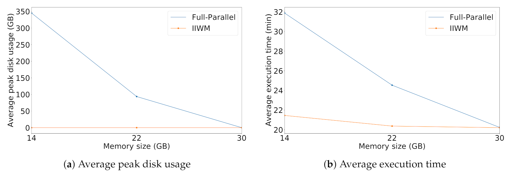
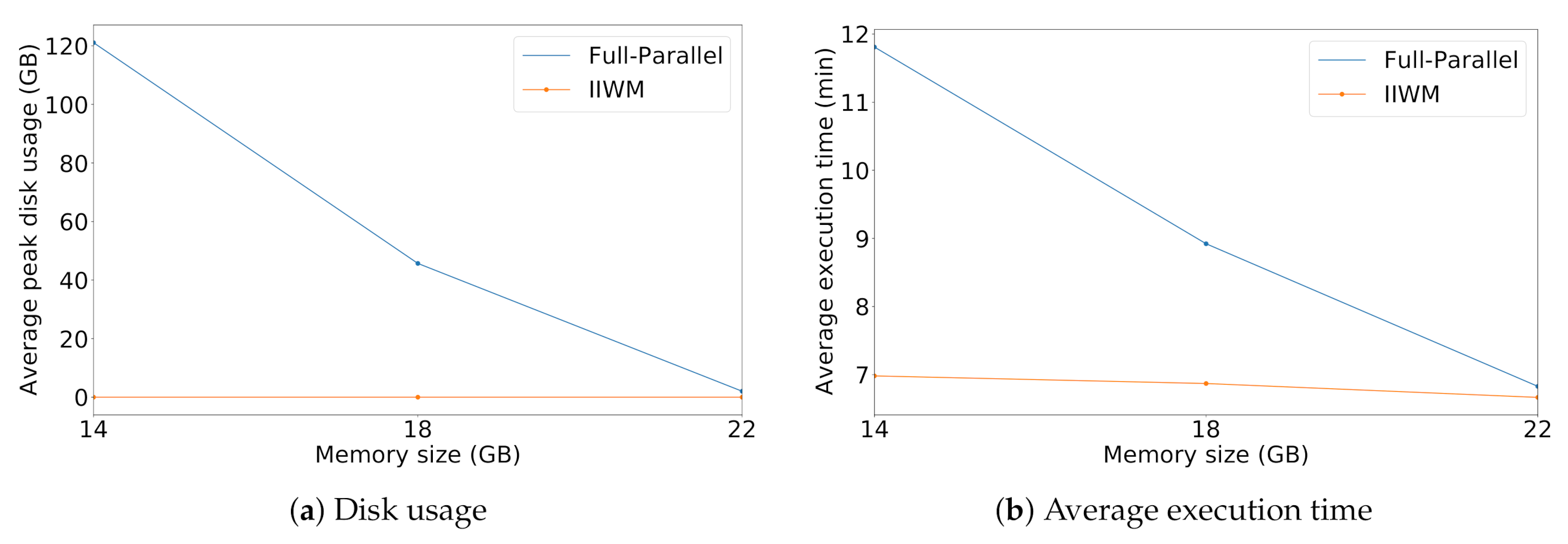
This section presents an experimental evaluation of the proposed system, aimed at optimizing the in-memory execution of data-intensive workflows. We experimentally assessed the effectiveness of the IIWM using Apache Spark 3.0.1 as a testbed. In particular, we generated two synthetic workflows for analyzing different scenarios, by assessing also the benefits coming from the use of the IIWM using a real data mining workflow as a case study.

In order to provide significant results, each experiment was executed ten times, and the average metrics with standard deviations are reported. In particular, for each experiment, we evaluated the accuracy of the regression model in predicting memory occupancy and execution time.

We evaluated the ability of the IIWM to improve application performance taking into account two different aspects:

• Execution time: Let $m_1$ and $m_2$ be the makespan for two different executions. If $m_2<m_1$, we can compute the improvement on makespan ($m_{imp}$) and application performance ($p_{imp}$) as follows:

  $$m_{imp}=\frac{m_1-m_2}{m_1}\times 100\%p_{imp}=\frac{m_1}{m_2}$$
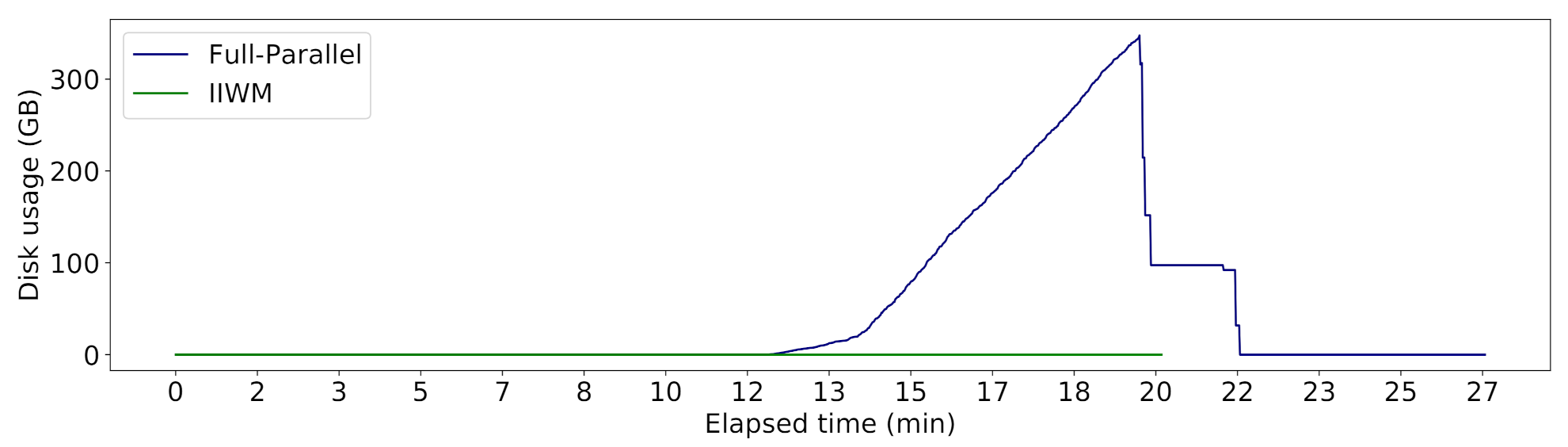
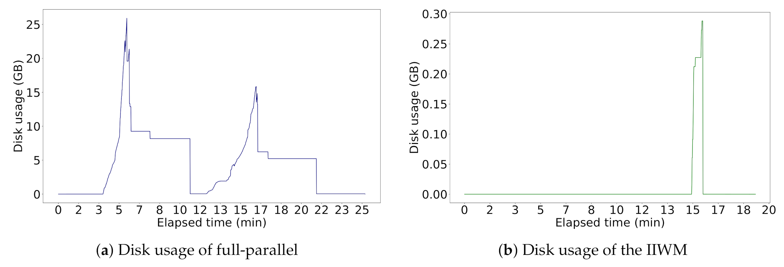
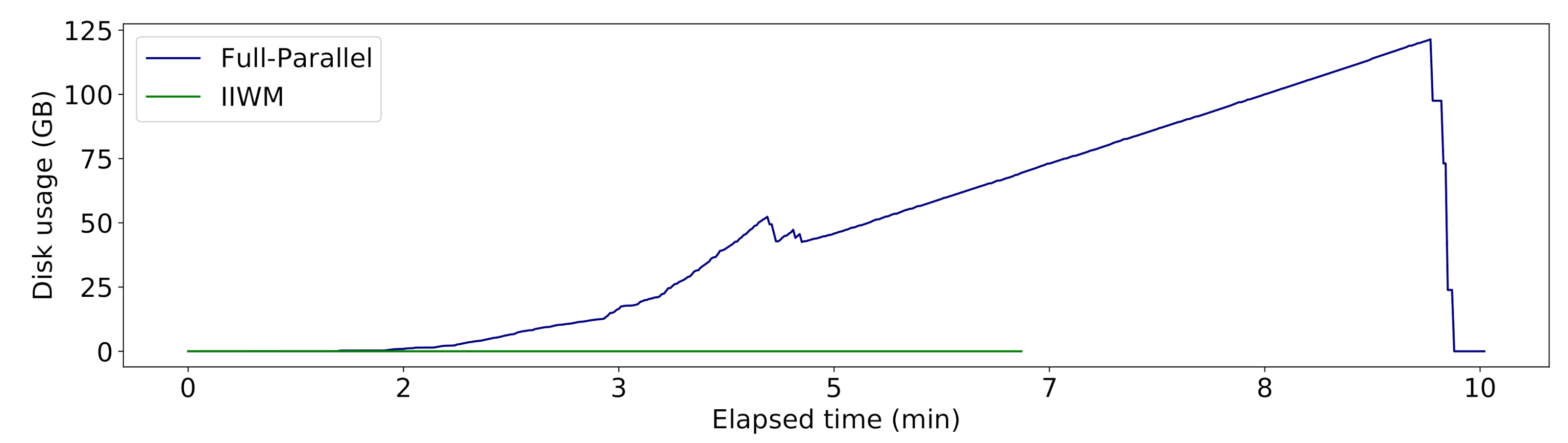
• Disk usage: We used the on-disk usage metric, which measures the amount of disk usage, jointly considering the volume and the duration of disk writes. Formally, given a sequence of disk writes $w_1,\dots ,w_k$, let ${\tau }_i^{{}^{\prime }}$, ${\tau }_i^{{}^{″}}\in \mathbb{T}$ be the start and end time of the $w_i$ write, respectively. Let also $W:\mathbb{T}\to \mathbb{R}$ be a function representing the amount of megabytes written to disk over time $\mathbb{T}$. We define on-disk usage as:

  $$on\text{-}diskusge=\sum _{i=1}^k\frac{1}{{\tau }_i^{″}-{\tau }_i^{\prime }}{\int }_{{\tau }_i^{\prime }}^{{\tau }_i^{″}}W\left(\tau \right)d\tau$$

Specifically, for each workflow, we reported: (i) a comparison between full-parallel and the IIWM in terms of disk usage over time; (ii) a detailed description of the scheduling plan generated by both strategies; (iii) the average improvement on makespan and application performance with the IIWM; (iv) statistics about the use of disk, such as the time spent for I/O operations and the on-disk usage metric; (v) the execution of the workflow by varying the amount of available memory, in order to show the benefits of the proposed scheduler in different limited memory scenarios.

4.1. Synthetic Workflows

We firstly evaluated our approach against two complex synthetic data analysis workflows, where the full-parallel approach showed its limitations due to a high degree of parallelism. The dependencies in these workflows should be understood as execution constraints. For instance, clustering has to be performed before classification for adding labels to an unlabeled dataset, or a classification task is performed after the discovery of association rules for user classification purposes.

The first test was carried out on a synthetic workflow with 42 nodes.

Table 6. Task and dataset descriptions (Workflow 1).

Node	Task Name	Task Type	Task Class	Rows	Columns	Categorical Columns	Dataset Size (MB)
$t_0$	Naive Bayes	Estimator	Classification	2,939,059	18	4	198.94
$t_1$	FPGrowth	Estimator	Association Rules	494,156	180	180	417.01
$t_2$	Naive Bayes	Estimator	Classification	5,000,000	27	0	321.86
$t_3$	K-Means	Estimator	Clustering	1,000,000	104	0	247.96
$t_4$	Decision Tree	Estimator	Classification	4,000,000	53	0	505.45
$t_5$	Decision Tree	Estimator	Classification	4,000,000	27	0	257.49
$t_6$	Decision Tree	Estimator	Classification	5,000,000	129	0	1542.58
$t_7$	K-Means	Estimator	Clustering	2,000,000	53	0	252.73
$t_8$	Naive Bayes	Estimator	Classification	2,000,000	104	0	495.90
$t_9$	Naive Bayes	Estimator	Classification	1,000,000	129	0	307.57
$t_{10}$	SVM	Estimator	Classification	2,000,000	53	0	252.72
$t_{11}$	K-Means	Estimator	Clustering	2,049,280	9	2	122.03
$t_{12}$	GMM	Estimator	Clustering	2,458,285	28	0	145.01
$t_{13}$	K-Means	Estimator	Clustering	9169	5812	1	101.89
$t_{14}$	SVM	Estimator	Classification	2,000,000	27	0	128.75
$t_{15}$	K-Means	Estimator	Clustering	3,000,000	104	0	743.87
$t_{16}$	SVM	Estimator	Classification	3,000,000	53	0	379.09
$t_{17}$	SVM	Estimator	Classification	14,410	1921	0	127.38
$t_{18}$	K-Means	Estimator	Clustering	5,000,000	53	0	631.81
$t_{19}$	K-Means	Estimator	Clustering	5,000,000	104	0	1239.78
$t_{20}$	K-Means	Estimator	Clustering	2,000,000	78	0	371.93
$t_{21}$	SVM	Estimator	Classification	3,000,000	104	0	743.87
$t_{22}$	K-Means	Estimator	Clustering	2,939,059	18	4	198.94
$t_{23}$	SVM	Estimator	Classification	19,213	1442	0	123.28
$t_{24}$	Decision Tree	Estimator	Classification	3,000,000	129	0	922.69
$t_{25}$	K-Means	Estimator	Clustering	1,959,372	26	4	189.55
$t_{26}$	Decision Tree	Estimator	Classification	4,898,431	18	4	331.57
$t_{27}$	Naive Bayes	Estimator	Classification	4,898,431	18	4	331.57
$t_{28}$	K-Means	Estimator	Clustering	2,939,059	34	4	334.91
$t_{29}$	K-Means	Estimator	Clustering	4,898,431	18	4	331.57
$t_{30}$	K-Means	Estimator	Clustering	1,966,628	42	0	170.49
$t_{31}$	Naive Bayes	Estimator	Classification	1,959,372	18	4	132.62
$t_{32}$	K-Means	Estimator	Clustering	3,000,000	78	0	557.91
$t_{33}$	Decision Tree	Estimator	Classification	3,000,000	53	0	379.09
$t_{34}$	Decision Tree	Estimator	Classification	14,410	2401	0	159.71
$t_{35}$	K-Means	Estimator	Clustering	2,939,059	42	4	386.53
$t_{36}$	Decision Tree	Estimator	Classification	2,939,059	34	4	334.91
$t_{37}$	Decision Tree	Estimator	Classification	4,000,000	129	0	1230.24
$t_{38}$	Naive Bayes	Estimator	Classification	1,000,000	53	0	126.36
$t_{39}$	GMM	Estimator	Clustering	1,000,000	53	0	126.36
$t_{40}$	Decision Tree	Estimator	Classification	2,939,059	18	4	198.94
$t_{41}$	K-Means	Estimator	Clustering	4,898,431	18	4	331.57

provides a detailed description of each task in the workflow, while their dependencies are shown in Figure 4.

The first step is to predict the memory occupancy and execution time of each task of the workflow: the regression model was able to accurately estimate the peaks on storage and execution memory and the duration, as shown in

Table 7. Performance evaluation of the prediction model.

	RMSE	MAE	Adjusted ${\mathit{R}}^2$	Pearson Correlation
Storage Memory	$246.63$	$95.6$	$0.96$	$0.98$
Execution Memory	$4.7$	$1.6$	$0.99$	$0.99$
Duration	20,354.38	7,877.72	$0.80$	$0.91$

.

We firstly considered a configuration characterized by 14 GB available for running the workflow, which was used up to $60\%$ due to the Spark unified memory model.

Table 8. Example of execution of Algorithm 1 at the iteration level.

Iteration	State	Stages
It. 0	${\mathcal{T}}_{free}^0=\left\{t_0\right\}$ Create $s_0$ and assign $t_0$ Unlock {$t_1,t_2,t_3$}	$s_0=\left\{t_0\right\}$
It. 1	${\mathcal{T}}_{free}^1=\{t_1,t_3,t_2\}$ Create $s_1$ and assign $t_1$ Unlock {$t_4$}	$s_0=\left\{t_0\right\}$, $s_1=\left\{t_1\right\}$
It. 2	${\mathcal{T}}_{free}^2=\{t_3,t_4,t_2\}$ Create $s_2$ and assign $t_3$ Unlock {$t_7,t_8,t_9,t_{10}$}	$s_0=\left\{t_0\right\}$, $s_1=\left\{t_1\right\}$, $s_2=\left\{t_3\right\}$
It. 3	${\mathcal{T}}_{free}^3=\{t_7,t_4,t_{10},t_2,t_8,t_9\}$ Create $s_3$ and assign $t_7$	$s_0=\left\{t_0\right\}$, $s_1=\left\{t_1\right\}$, $s_2=\left\{t_3\right\}$, $s_3=\left\{t_7\right\}$
It. 4	${\mathcal{T}}_{free}^4=\{t_4,t_{10},t_2,t_8,t_9\}$ ${\mathcal{S}}_{sel}=\{s_2,s_3\}$ $increase=\{0,0\}$ Assign $t_4$ to $s_2$	$s_0=\left\{t_0\right\}$, $s_1=\left\{t_1\right\}$, $s_2=\{t_3,t_4\}$, $s_3=\left\{t_7\right\}$
⋯	⋯	⋯
It. 17	${\mathcal{T}}_{free}^{17}=\{t_{17},t_{23},t_8,t_9\}$ ${\mathcal{S}}_{sel}=\{s_6,s_7\}$ $increase=\{12,496.36,0\}$ Assign $t_{17}$ to $s_7$ Unlock {$t_{25}$}	$s_0=\left\{t_0\right\}$, $s_1=\{t_1,t_2\}$, $s_2=\{t_3,t_4,t_5\}$, $s_3=\{t_7,t_{10},t_6\}$, $s_4=\{t_{12},t_{11}\}$, $s_5=\{t_{15},t_{18}\}$, $s_6=\{t_{19},t_{22}\}$, $s_7=\{t_{24},t_{16},t_{17}\}$
⋯	⋯	⋯

shows an execution example with the IIWM, focusing on its main steps: (i) the scheduling of tasks based on their decreasing memory weight; (ii) the allocation of a new stage; (iii) the exploitation of the estimated execution time while computing the marginal increase. This last aspect can be clearly observed in Iteration 17, where task $t_{17}$ is assigned to stage $s_7$, which presents a marginal increase equal to zero. This is the best choice compared to the other candidate stage ($s_6$), whose execution time would be increased by 12,496.36 milliseconds by the assignment of $t_{17}$, with a degradation of the overall makespan.

At the end of the process, a consolidation step is exploited for optimizing throughput and execution time, by merging two stages with zero out-degree with some tailing stages, so as to avoid the sequential execution of the two stages in favor of a parallel one.

Figure 5 shows disk occupancy throughout the execution. As a consequence of memory saturation, the execution of full-parallel resulted in a huge amount of disk writes, while IIWM achieved a null disk usage since no swapping occurred thanks to intelligent task scheduling. Thus, this translates into better use of in-memory computing.

These results can be clearly seen also in

Table 9. Scheduling plan and statistics about execution times and disk usage with 14 GB of RAM.

Strategy	Task-Scheduling Plan	Number of Stages	Time (min)	Peak Disk Usage (MB)	Writes Duration (min)	On-Disk Usage (MB)
Full-Parallel	($t_0$), ($t_1$ ‖ $t_2$ ‖ $t_3$), ($t_4$ ‖ $t_5$ ‖ $t_6$ ‖ $t_7$ ‖ $t_8$ ‖ $t_9$ ‖ $t_{10}$), ($t_{11}$ ‖ $t_{12}$ ‖ $t_{13}$ ‖ $t_{14}$), ($t_{15}$ ‖ $t_{16}$ ‖ $t_{17}$ ‖ $t_{18}$ ‖ $t_{19}$ ‖ $t_{20}$ ‖ $t_{21}$), ($t_{22}$ ‖ $t_{23}$ ‖ $t_{24}$ ‖ $t_{25}$ ‖ $t_{26}$ ‖ $t_{27}$ ‖ $t_{28}$), ($t_{29}$ ‖ $t_{30}$ ‖ $t_{31}$ ‖ $t_{32}$ ‖ $t_{33}$ ‖ $t_{34}$ ‖ $t_{41}$), ($t_{35}$ ‖ $t_{36}$ ‖ $t_{37}$), ($t_{38}$ ‖ $t_{39}$), ($t_{40}$)	10	$31.52\pm 0.6$	356,106.60	$11.56$	126,867.06
IIWM	($t_0$), ($t_1$ ‖ $t_2$), ($t_3$ ‖ $t_4$ ‖ $t_5$), ($t_7$ ‖ $t_{10}$ ‖ $t_6$ ‖ $t_8$ ‖ $t_9$), ($t_{12}$ ‖ $t_{11}$ ‖ $t_{13}$), ($t_{15}$ ‖ $t_{18}$), ($t_{19}$ ‖ $t_{22}$ ‖ $t_{23}$), ($t_{24}$ ‖ $t_{16}$ ‖ $t_{17}$ ‖ $t_{29}$), ($t_{25}$ ‖ $t_{41}$), ($t_{30}$ ‖ $t_{20}$), ($t_{35}$ ‖ $t_{21}$ ‖ $t_{14}$), ($t_{28}$ ‖ $t_{26}$ ‖ $t_{27}$), ($t_{33}$ ‖ $t_{32}$ ‖ $t_{34}$ ‖ $t_{31}$), ($t_{37}$ ‖ $t_{36}$), ($t_{39}$ ‖ $t_{38}$), ($t_{40}$)	16	$21.70\pm 0.63$	0	0	0

, which shows the scheduling plan produced by the IIWM scheduler, together with some statistics about the execution times and the use of the disk. In particular, given the curves representing disk writes over time shown in Figure 5, on-disk usage graphically represents the sum, for each disk write, of the ratio between the area under the curve identified by a write and its duration. Compared to the full-parallel strategy, the IIWM achieved better execution times and an improvement in application performance, with a boost of almost $1.45x$ ($p_{imp}$) and a $31.15\%$ reduction in time ($m_{imp}$) on average.

With different sizes of available memory, the full-parallel approach showed higher and higher execution times and disk writes as memory decreased, while the IIWM was able to adapt the execution to available resources, as shown in Figure 6, finding a good trade-off between the maximization of the parallelism and the minimization of the memory saturation probability. At the extremes, with unlimited available memory, or at least greater than that required to run the workflow, the IIWM performs as a full concurrent strategy, producing the same scheduling of full-parallel.

The second synthetic workflow consisted of the 27 tasks described by

Table 10. Task and dataset descriptions (Workflow 2).

Node	Task Name	Task Type	Task Class	Rows	Columns	Categorical Columns	Dataset Size (MB)
$t_0$	K-Means	Estimator	Clustering	3,918,745	34	4	446.55
$t_1$	Decision Tree	Estimator	Classification	4,000,000	27	0	257.49
$t_2$	GMM	Estimator	Clustering	2,458,285	28	0	145.01
$t_3$	Decision Tree	Estimator	Classification	3,000,000	53	0	379.09
$t_4$	Decision Tree	Estimator	Classification	4,000,000	129	0	1230.24
$t_5$	Decision Tree	Estimator	Classification	3,918,745	18	4	265.25
$t_6$	Decision Tree	Estimator	Classification	4,898,431	42	3	648.89
$t_7$	Decision Tree	Estimator	Classification	2,939,059	42	4	386.53
$t_8$	K-Means	Estimator	Clustering	2,458,285	56	0	278.75
$t_9$	GMM	Estimator	Clustering	3,000,000	53	0	379.09
$t_{10}$	SVM	Estimator	Classification	4,000,000	53	0	505.45
$t_{11}$	K-Means	Estimator	Clustering	2,939,059	42	4	386.53
$t_{12}$	SVM	Estimator	Classification	2,000,000	53	0	252.72
$t_{13}$	K-Means	Estimator	Clustering	1,639,424	9	2	93.70
$t_{14}$	Naive Bayes	Estimator	Classification	260,924	3	0	10.33
$t_{15}$	K-Means	Estimator	Clustering	2,000,000	78	0	371.93
$t_{16}$	Decision Tree	Estimator	Classification	3,918,745	26	4	379.11
$t_{17}$	Decision Tree	Estimator	Classification	3,918,745	34	4	446.55
$t_{18}$	FPGrowth	Estimator	Association Rules	823,593	180	180	697.00
$t_{19}$	Decision Tree	Estimator	Classification	2,939,059	26	4	284.33
$t_{20}$	SVM	Estimator	Classification	5,000,000	27	0	321.86
$t_{21}$	FPGrowth	Estimator	Association Rules	164,719	180	180	139.87
$t_{22}$	GMM	Estimator	Clustering	3,000,000	27	0	193.12
$t_{23}$	K-Means	Estimator	Clustering	4,898,431	26	4	473.88
$t_{24}$	Decision Tree	Estimator	Classification	2,000,000	104	0	495.90
$t_{25}$	K-Means	Estimator	Clustering	2,458,285	69	0	344.60
$t_{26}$	FPGrowth	Estimator	Association Rules	494,156	180	180	417.01

and their dependencies, shown in Figure 7. This scenario was characterized by highly heavy tasks and very low resources, where the execution of a single task can exceed the available memory. In particular, the task $T_{18}$ had an estimated peak memory occupancy higher than Spark’s available unified memory of $5413.8$ MB (i.e., corresponding to a heap size of $9.5$ GB): this would bring the IIWM scheduling algorithm to allocate the task to a new stage, but memory would be saturated anyway.

In such a situation, data spilling to disk cannot be avoided, but the IIWM tries to minimize the number of bytes written and the duration of I/O operations. Even in this scenario, the prediction model achieved very accurate results, shown in

Table 11. Performance evaluation of the prediction model.

	RMSE	MAE	Adjusted ${\mathit{R}}^2$	Pearson Correlation
Storage Memory	$213.81$	$78.92$	$0.98$	$0.99$
Execution Memory	$29.86$	$11.56$	$0.98$	$0.99$
Duration	20,086.80	9925.13	$0.82$	$0.94$

, confirming its forecasting abilities.

Figure 8 shows the disk occupancy during the execution. As we can see, even the IIWM could not avoid data spilling, even though its disk usage was much lower considering the peak value and write duration compared to full-parallel.

Finally,

Table 12. Scheduling plan and statistics about execution times and disk usage with 9.5 GB of RAM.

Strategy	Task-Scheduling Plan	Number of Stages	Time (min)	Peak Disk Usage (MB)	Writes Duration (min)	On-Disk Usage (MB)
Full-Parallel	($t_0$), ($t_1$ ‖ $t_2$ ‖ $t_3$ ‖ $t_4$), ($t_5$ ‖ $t_6$ ‖ $t_7$ ‖ $t_8$ ‖ $t_9$ ‖ $t_{10}$ ‖ $t_{11}$ ‖ $t_{12}$), ($t_{13}$ ‖ $t_{14}$ ‖ $t_{15}$ ‖ $t_{16}$ ‖ $t_{17}$ ‖ $t_{18}$ ‖ $t_{19}$ ‖ $t_{20}$), ($t_{21}$), ($t_{22}$ ‖ $t_{23}$ ‖ $t_{24}$ ‖ $t_{25}$), ($t_{26}$)	7	$29.42\pm 1.88$	27,095.84	$20.6$	10,593.79
IIWM	($t_0$), ($t_4$ ‖ $t_2$), ($t_{11}$ ‖ $t_7$), ($t_8$ ‖ $t_3$), ($t_{15}$ ‖ $t_{10}$ ‖ $t_9$ ‖ $t_{16}$), ($t_{18}$), ($t_{17}$ ‖ $t_1$ ‖ $t_{12}$), ($t_6$ ‖ $t_5$), ($t_{14}$), ($t_{13}$ ‖ $t_{20}$ ‖ $t_{19}$), ($t_{21}$), ($t_{23}$ ‖ $t_{24}$), ($t_{25}$), ($t_{22}$), ($t_{26}$)	15	$22.68\pm 1.65$	$304.5$	$3.6$	$60.82$

shows the statistics about disk usage and execution times. Again, the IIWM achieved better results with a boost in performance of almost $1.30\times$ ($p_{imp}$) with respect to a full-parallel strategy and a $23\%$ reduction in time ($m_{imp}$) on average. An interesting aspect that emerged from the behavior of the IIWM scheduler, in the task-scheduling plan, was the similarity with priority-based scheduling in assigning tasks based on decreasing weights. In fact, tasks characterized by low memory occupancy may be assigned to tailing stages even if they are close to the root (e.g., in full-parallel, $t_1$ is executed in the second stage, while in the IIWM, it is executed in the seventh one). Hence, in a dynamic scheduling scenario where tasks can be added at runtime, the IIWM may suffer from the starvation problem, as such tasks may experience an indefinite delay as far as new tasks with a higher memory weight are provided to the scheduler. Nevertheless, in the proposed work, we dealt with a static scheduling problem, where all tasks were known in advance and the task set was not modifiable at runtime.

4.2. Real Case Study

In order to assess the performance of the proposed approach against a real case study, we used a data mining workflow [27] that implements a model selection strategy for the classification of an unlabeled dataset. Figure 9 shows a representation of the workflow designed by the visual language VL4Cloud [28]. The training set was divided into n partitions, and k classification algorithms were fit on each partition for generating $k\times n$ classification models. The $k\times n$ fit models were evaluated by a model selector on a test set to choose the best model. Afterwards, the n predictors used the best model to generate n classified datasets. The following k classification algorithms provided by the MLlib library were used: decision tree with C4.5 algorithm, Support Vector Machines (SVMs), and naive Bayes. The training set, test set, and unlabeled dataset provided as the input for the workflow were generated from the Physical Unclonable Functions (PUFs) [29] simulation through an n-fold-cross strategy. In this scenario, the IIWM can be used to optimize the data processing phase regarding the execution of the $k\times n$ classification algorithms (estimators first, transformers second) concurrently. The other phases, such as data acquisition and partitioning, were outside our interest. The red box in Figure 9 shows the tasks of the workflow that were analyzed.

Figure 10 shows disk occupancy over time with 14 GB of RAM. In this case as well, the IIWM avoided disk writes, while full-parallel registered a high level of disk usage. In particular, during the training phase, the parallel execution of the $k\times n$ models (with $k=3$ and $n=5$) saturated memory with 15 concurrent tasks and generated disk writes up to 124 GB.

The results are detailed in

Table 13. Scheduling plan and statistics about execution times and disk usage with 14 GB of RAM.

Strategy	Task-Scheduling Plan	Number of Stages	Time (min)	Peak Disk Usage (MB)	Writes Duration (min)	On-Disk Usage (MB)
Full-Parallel	($t_0$ ‖ $t_2$ ‖ $t_4$ ‖ $t_6$ ‖ $t_8$ ‖ $t_{10}$ ‖ $t_{12}$ ‖ $t_{14}$ ‖ $t_{16}$ ‖ $t_{18}$ ‖ $t_{20}$ ‖ $t_{22}$ ‖ $t_{24}$ ‖ $t_{26}$ ‖ $t_{28}$), ($t_1$ ‖ $t_3$ ‖ $t_5$ ‖ $t_7$ ‖ $t_9$ ‖ $t_{11}$ ‖ $t_{13}$ ‖ $t_{15}$ ‖ $t_{17}$ ‖ $t_{19}$ ‖ $t_{21}$ ‖ $t_{23}$ ‖ $t_{25}$ ‖ $t_{27}$ ‖ $t_{29}$)	2	$11.42\pm 0.27$	124,730.87	$9.6$	54,443.19
IIWM	($t_{10}$ ‖ $t_{12}$ ‖ $t_{14}$ ‖ $t_{16}$ ‖ $t_{20}$ ‖ $t_{22}$ ‖ $t_{24}$ ‖ $t_{26}$ ‖ $t_{28}$), ($t_{18}$ ‖ $t_0$ ‖ $t_2$ ‖ $t_4$ ‖ $t_6$ ‖ $t_8$ ‖ $t_{11}$ ‖ $t_{13}$ ‖ $t_{15}$ ‖ $t_{17}$ ‖ $t_{21}$ ‖ $t_{23}$ ‖ $t_{25}$ ‖ $t_{27}$ ‖ $t_{29}$), ($t_{19}$ ‖ $t_1$ ‖ $t_3$ ‖ $t_5$ ‖ $t_7$ ‖ $t_9$)	3	$6.88\pm 0.1$	0	0	0

, which shows a boost in execution time of almost $1.66\times$ ($p_{imp}$) and a $40\%$ time reduction ($m_{imp}$) with respect to full-parallel.

The general trends varying the amount of available resources were also confirmed with respect to the previous examples, as shown in Figure 11.

5. Conclusions and Final Remarks

Currently, data-intensive workflows are widely used in several application domains, such as bioinformatics, astronomy, and engineering. This paper introduced and evaluated a system, named the Intelligent In-memory Workflow Manager (IIWM), aimed at optimizing the in-memory execution of data-intensive workflows on high-performance computing systems. Experimental results suggested that by jointly using a machine learning model for performance estimation and a suitable scheduling strategy, the execution of data-intensive workflows can be significantly improved with respect to state-of-the-art blind strategies. In particular, the main benefits of the IIWM resulted when it was applied to workflows having a high level of parallelism. In this case, a significant reduction of memory saturation was obtained. Therefore, it can be used effectively when multiple tasks have to be executed on the same computing node, for example when they need to be run on multiple immovable datasets located on a single node or due to other hardware constraints. In these cases, an uninformed scheduling strategy will likely exceed the available memory, causing disk writes and, therefore, a drop in performance. The proposed approach was also shown to be a very suitable solution in scenarios characterized by a limited amount of memory reserved for execution, thus finding possible applications in data-intensive IoT workflows, where data processing is performed on constrained devices located at the network edge.

The IIWM was evaluated against different scenarios concerning both synthetic and real data mining workflows, using Apache Spark as a testbed. Specifically, by accurately predicting the resources used at runtime, our approach achieved up to a $31\%$ and a $40\%$ reduction of makespan and a performance improvement up to $1.45\times$ and $1.66\times$ on the synthetic workflows and the real case study, respectively.

In future work, additional aspects of the performance estimation will be investigated. For example, IIWM can be extended also to consider: (i) other common stages in workflows besides data analysis, such as data acquisition, integration, and reduction; (ii) more complex algorithms like Artificial Neural Networks or Random Forests; (iii) other information about tasks, input data, and hardware platform features.

References yes

References

1. Talia, D.; Trunfio, P.; Marozzo, F. Data Analysis in the Cloud; Elsevier: Amsterdam, The Netherlands, 2015; ISBN 978-0-12-802881-0. [Google Scholar]
2. Da Costa, G.; Fahringer, T.; Rico-Gallego, J.A.; Grasso, I.; Hristov, A.; Karatza, H.D.; Lastovetsky, A.; Marozzo, F.; Petcu, D.; Stavrinides, G.L.; et al. Exascale machines require new programming paradigms and runtimes. Supercomput. Front. Innov. 2015, 2, 6–27. [Google Scholar]
3. Li, M.; Tan, J.; Wang, Y.; Zhang, L.; Salapura, V. SparkBench: A Comprehensive Benchmarking Suite for in Memory Data Analytic Platform Spark. In Proceedings of the 12th ACM International Conference on Computing Frontiers, Ischia, Italy, 18–21 May 2015; Association for Computing Machinery: New York, NY, USA, 2015. [Google Scholar] [CrossRef]
4. De Oliveira, D.C.; Liu, J.; Pacitti, E. Data-intensive workflow management: For clouds and data-intensive and scalable computing environments. Synth. Lect. Data Manag. 2019, 14, 1–179. [Google Scholar] [CrossRef]
5. Verma, A.; Mansuri, A.H.; Jain, N. Big data management processing with Hadoop MapReduce and spark technology: A comparison. In Proceedings of the 2016 Symposium on Colossal Data Analysis and Networking (CDAN), Indore, India, 18–19 March 2016; pp. 1–4. [Google Scholar] [CrossRef]
6. Zaharia, M.; Chowdhury, M.; Das, T.; Dave, A.; Ma, J.; McCauly, M.; Franklin, M.J.; Shenker, S.; Stoica, I. Resilient distributed datasets: A fault-tolerant abstraction for in-memory cluster computing. In Proceedings of the 9th USENIX Symposium on Networked Systems Design and Implementation (NSDI 12), San Jose, CA, USA, 25–27 April 2012; pp. 15–28. [Google Scholar]
7. Samadi, Y.; Zbakh, M.; Tadonki, C. Performance comparison between Hadoop and Spark frameworks using HiBench benchmarks. Concurr. Comput. Pract. Exp. 2018, 30, e4367. [Google Scholar] [CrossRef]
8. Delimitrou, C.; Kozyrakis, C. Quasar: Resource-Efficient and QoS-Aware Cluster Management. In Proceedings of the 19th International Conference on Architectural Support for Programming Languages and Operating Systems, Salt Lake City, UT, USA, 1–5 March 2014; Association for Computing Machinery: New York, NY, USA, 2014; pp. 127–144. [Google Scholar] [CrossRef]
9. Llull, Q.; Fan, S.; Zahedi, S.M.; Lee, B.C. Cooper: Task Colocation with Cooperative Games. In Proceedings of the 2017 IEEE International Symposium on High Performance Computer Architecture (HPCA), Austin, TX, USA, 4–8 February 2017; pp. 421–432. [Google Scholar] [CrossRef]
10. Marco, V.S.; Taylor, B.; Porter, B.; Wang, Z. Improving Spark Application Throughput via Memory Aware Task Co-Location: A Mixture of Experts Approach. In Proceedings of the 18th ACM/IFIP/USENIX Middleware Conference, Las Vegas, NV, USA, 11–15 December 2017; Association for Computing Machinery: New York, NY, USA, 2017. Middleware’17. pp. 95–108. [Google Scholar] [CrossRef] [Green Version]
11. Maros, A.; Murai, F.; Couto da Silva, A.P.; Almeida, J.M.; Lattuada, M.; Gianniti, E.; Hosseini, M.; Ardagna, D. Machine Learning for Performance Prediction of Spark Cloud Applications. In Proceedings of the 2019 IEEE 12th International Conference on Cloud Computing (CLOUD), Milan, Italy, 8–13 July 2019; pp. 99–106. [Google Scholar] [CrossRef] [Green Version]
12. Talia, D. Workflow Systems for Science: Concepts and Tools. Int. Sch. Res. Not. 2013, 2013, 404525. [Google Scholar] [CrossRef] [Green Version]
13. Smanchat, S.; Viriyapant, K. Taxonomies of workflow scheduling problem and techniques in the cloud. Future Gener. Comput. Syst. 2015, 52, 1–12. [Google Scholar] [CrossRef]
14. Bittencourt, L.F.; Madeira, E.R.M.; Da Fonseca, N.L.S. Scheduling in hybrid clouds. IEEE Commun. Mag. 2012, 50, 42–47. [Google Scholar] [CrossRef]
15. Zhao, Y.; Hu, F.; Chen, H. An adaptive tuning strategy on spark based on in-memory computation characteristics. In Proceedings of the 2016 18th International Conference on Advanced Communication Technology (ICACT), Pyeongchang, Korea, 31 January–3 February 2016; pp. 484–488. [Google Scholar] [CrossRef]
16. Chen, D.; Chen, H.; Jiang, Z.; Zhao, Y. An adaptive memory tuning strategy with high performance for Spark. Int. J. Big Data Intell. 2017, 4, 276–286. [Google Scholar] [CrossRef]
17. Xuan, P.; Luo, F.; Ge, R.; Srimani, P.K. Dynamic Management of In-Memory Storage for Efficiently Integrating Compute-and Data-Intensive Computing on HPC Systems. In Proceedings of the 2017 17th IEEE/ACM International Symposium on Cluster, Cloud and Grid Computing (CCGRID), Madrid, Spain, 14–17 May 2017; pp. 549–558. [Google Scholar] [CrossRef]
18. Tang, Z.; Zeng, A.; Zhang, X.; Yang, L.; Li, K. Dynamic memory-aware scheduling in spark computing environment. J. Parallel Distrib. Comput. 2020, 141, 10–22. [Google Scholar] [CrossRef]
19. Bae, J.; Jang, H.; Jin, W.; Heo, J.; Jang, J.; Hwang, J.; Cho, S.; Lee, J.W. Jointly optimizing task granularity and concurrency for in-memory mapreduce frameworks. In Proceedings of the 2017 IEEE International Conference on Big Data (Big Data), Boston, MA, USA, 11–14 December 2017; pp. 130–140. [Google Scholar] [CrossRef]
20. Wolpert, D.H. Stacked generalization. Neural Netw. 1992, 5, 241–259. [Google Scholar] [CrossRef]
21. Liu, J.; Pacitti, E.; Valduriez, P.; Mattoso, M. A Survey of Data-Intensive Scientific Workflow Management. J. Grid Comput. 2015, 13, 457–493. [Google Scholar] [CrossRef]
22. Raj, P.H.; Kumar, P.R.; Jelciana, P. Load Balancing in Mobile Cloud Computing using Bin Packing’s First Fit Decreasing Method. In Proceedings of the International Conference on Computational Intelligence in Information System, Brunei, 16–18 November 2018; Springer: Berlin, Germany, 2018; pp. 97–106. [Google Scholar]
23. Baker, T.; Aldawsari, B.; Asim, M.; Tawfik, H.; Maamar, Z.; Buyya, R. Cloud-SEnergy: A bin-packing based multi-cloud service broker for energy efficient composition and execution of data-intensive applications. Sustain. Comput. Informatics Syst. 2018, 19, 242–252. [Google Scholar] [CrossRef] [Green Version]
24. Stavrinides, G.L.; Karatza, H.D. Scheduling real-time DAGs in heterogeneous clusters by combining imprecise computations and bin packing techniques for the exploitation of schedule holes. Future Gener. Comput. Syst. 2012, 28, 977–988. [Google Scholar] [CrossRef]
25. Coffman, E.G., Jr.; Garey, M.R.; Johnson, D.S. An application of bin-packing to multiprocessor scheduling. SIAM J. Comput. 1978, 7, 1–17. [Google Scholar] [CrossRef]
26. Darapuneni, Y.J. A Survey of Classical and Recent Results in Bin Packing Problem. UNLV Theses, Dissertations, Professional Papers, and Capstones. 2012. Available online: https://digitalscholarship.unlv.edu/cgi/viewcontent.cgi?article=2664&context=thesesdissertations (accessed on 29 April 2021).
27. Marozzo, F.; Rodrigo Duro, F.; Garcia Blas, J.; Carretero, J.; Talia, D.; Trunfio, P. A data-aware scheduling strategy for workflow execution in clouds. Concurr. Comput. Pract. Exp. 2017, 29, e4229. [Google Scholar] [CrossRef]
28. Marozzo, F.; Talia, D.; Trunfio, P. A Workflow Management System for Scalable Data Mining on Clouds. IEEE Trans. Serv. Comput. 2018, 11, 480–492. [Google Scholar] [CrossRef]
29. Aseeri, A.O.; Zhuang, Y.; Alkatheiri, M.S. A Machine Learning-Based Security Vulnerability Study on XOR PUFs for Resource-Constraint Internet of Things. In Proceedings of the 2018 IEEE International Congress on Internet of Things (ICIOT), San Francisco, CA, USA, 2–7 July 2018; pp. 49–56. [Google Scholar] [CrossRef]
Figure 1. Correlation of target variables with the other features.
Futureinternet 13 00121 g001
Figure 2. Meta learner regression estimates for the different target variables.
Futureinternet 13 00121 g002
Figure 3. Execution flow of the IIWM scheduler. Given a workflow and a prediction model as the input, a scheduling plan is generated in two steps: (i) building of the stages and task assignment; (ii) stage consolidation.
Futureinternet 13 00121 g003
Figure 4. Task dependencies (Workflow 1).
Futureinternet 13 00121 g004
Figure 5. Disk usage over time for full-parallel and the IIWM.
Futureinternet 13 00121 g005
Figure 6. Average peak disk usage and execution time, varying the size of available memory.
Futureinternet 13 00121 g006
Figure 7. Task dependencies (Workflow 2).
Futureinternet 13 00121 g007
Figure 8. Disk usage over time for full-parallel and the IIWM.
Futureinternet 13 00121 g008
Figure 9. Ensemble learning workflow.
Futureinternet 13 00121 g009
Figure 10. Disk usage over time for full-parallel and the IIWM.
Futureinternet 13 00121 g010
Figure 11. Average peak disk usage and execution time, varying the size of available memory.
Futureinternet 13 00121 g011