
A Fusion-Based Hybrid-Feature Approach for Recognition of Unconstrained Offline Handwritten Hindi Characters

 , ,
, ,  ,
,  and
and
Abstract
:1. Introduction
1.1. Related Work
1.2. Motivation
- To introduce the novel approach of handwritten Hindi character recognition with the benefits of features received from pre-trained DCNN models, accompanied by the reduced computational loads of the classifiers.
- The majority of previously reported works have been solely based on either handcrafted features or CNN-based features. No work has been reported yet in which both types of features are used in a single feature-vector for the recognition of handwritten Hindi characters. CNN-based features and handcrafted features have their own advantages—the former are auto-generative and the latter are rich in customization.
- The model performance for each character-class of Hindi script has also not been covered in detail, such as character-wise correct and incorrect predictions; the amount of false-positive and false-negative predictions out of the total incorrect predictions and development of a confusion-matrix for all the 36 classes of Hindi consonants, etc.
- The examination of the effectiveness of individual feature-types and their all-possible combinations is also a novel approach in relation to handwritten Hindi characters.
1.3. Contribution
- The scheme exploited pre-trained DCNN models, namely Inception-Net, VGG-NET, and Res-Net for feature extraction from the handwritten character-images; due to their excellent performance in the ImageNet Large Scale Visual Recognition Challenge (ILSVRC) annual competition [34].
- The model experimented with the fresh approach of feature–fusion, where the features received from pre-trained DCNN models were fused with the features received from handcrafted methods. In the proposed scheme, Bi-orthogonal Discrete Wavelet Transform (BDWT) was the natural choice for handcrafted features because of its properties like flexibility, separability, scalability, and transformability with the power of multi-resolution analysis. A very limited work has been reported on the use of DWT for the recognition of handwritten Hindi characters [27,35]. The effective PCA method was implemented in the proposed work for dimensionality reduction of feature-vectors by preserving most of the important details. This helped in achieving a low computational cost.
- The proposed scheme has thoroughly investigated the performance of the model for individual character-class. The number of performance metrics like precision, recall, and F1-measure was evaluated for the test samples of each character class to determine the amount of correct and incorrect recognitions. A confusion matrix was generated for precise character-wise result analysis.
- The strength of individual feature-types present in the hybrid-feature-vector and their all-possible combinations were evaluated for recognition accuracy.
- The proposed features were examined with two popular classifiers, namely MLP and SVM. This was done to examine the performance of proposed features over ANN-based and kernel-based approaches, respectively, for the given multiclass problem.
- Various timings, related to feature-extraction and character-recognition, were estimated in the proposed work.
2. Preliminary
2.1. Transfer Learning
2.1.1. VGG-19Net
2.1.2. Inception V3-Net
2.1.3. ResNet-50
2.2. Handcrafted Features: Bi-Orthogonal Discrete Wavelet Transform
2.3. Principal Component Analysis
2.4. Multi Layer Perceptron
2.5. Support Vector Machine
3. Research Method
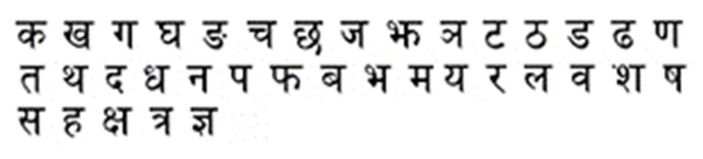
3.1. Dataset Pre-Processing
3.2. Feature Extraction
3.2.1. Discrete Wavelet Transform
3.2.2. Pre-Trained Deep Convolutional Network
3.3. Feature-Vector Size Reduction
3.4. Fusion of Features
3.5. Classification
3.6. Performance Metrics
4. Results and Discussions
4.1. Results
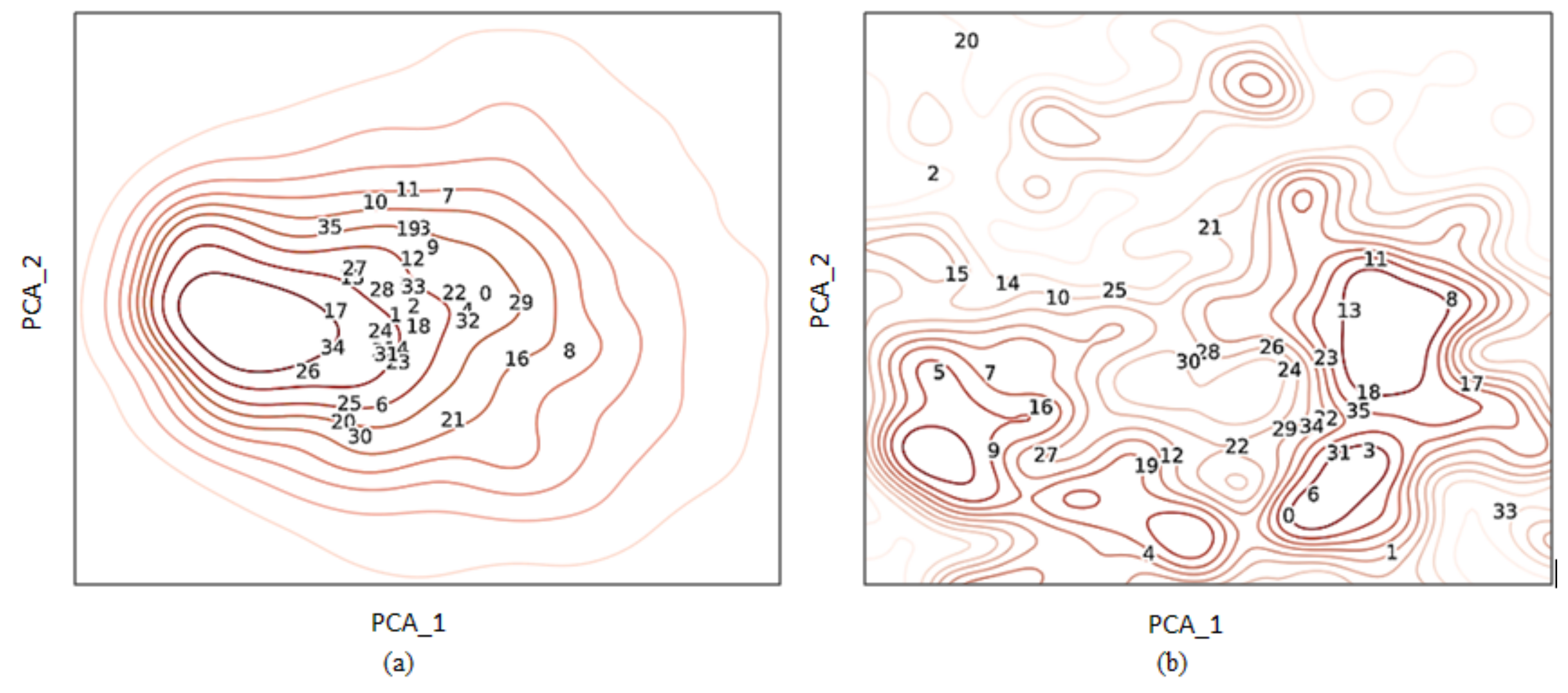
4.1.1. Feature Visualization
4.1.2. Estimation of Computational Time
4.2. Discussions
4.2.1. Feature-Wise Discussion
4.2.2. Classifier-Wise Discussion
4.2.3. Character-Wise Discussion
5. Conclusions
Author Contributions
Funding
Data Availability Statement
Conflicts of Interest
References
- Memon, J.; Sami, M.; Khan, R.A.; Uddin, M. Handwritten Optical Character Recognition (OCR): A Comprehensive Systematic Literature Review (SLR). IEEE Access 2020, 8, 142642–142668. [Google Scholar] [CrossRef]
- Yadav, M.; Purwar, R.K.; Mittal, M. Handwritten Hindi character recognition: A review. IET Image Process. 2018, 12, 1919–1933. [Google Scholar] [CrossRef]
- Sharma, R.; Kaushik, B. Offline recognition of handwritten Indic scripts: A state-of-the-art survey and future perspectives. Comput. Sci. Rev. 2020, 38, 100302. [Google Scholar] [CrossRef]
- Jayadevan, R.; Kolhe, S.R.; Patil, P.M.; Pal, U. Offline Recognition of Devanagari Script: A Survey. IEEE Trans. Syst. MAN Cybern. C Appl. Rev. 2011, 41, 782–796. [Google Scholar] [CrossRef]
- Sethi, I.K.; Chatterjee, B. Machine Recognition of Hand-printed Devnagri Numerals. IETE J. Res. 1976, 22, 532–535. [Google Scholar] [CrossRef]
- Bhattacharya, U.; Parui, S.K.; Shaw, B.; Bhattacharya, K. Neural Combination of ANN and HMM for Handwritten Devanagari Numeral Recognition. In Proceedings of the Tenth International Workshop on Frontiers in Handwriting Recognition, La Baule, France, October 2006; Suvisoft: Tampre, Finland, 2006. [Google Scholar]
- Arora, S.; Bhattacharjee, D.; Nasipuri, M.; Malik, L. A Two Stage Classification Approach for Handwritten Devanagari Characters. In Proceedings of the International Conference on Computational Intelligence and Multimedia Applications 2007, Sivakasi, India, 13–15 December 2007; IEEE Press: Piscataway, NJ, USA, 2007; pp. 404–408. [Google Scholar]
- Bajaj, R.; Dey, L.; Chaudhury, S. Devnagari numeral recognition by combining decision of multiple connectionist classifiers. Sadhana 2002, 27, 59–72. [Google Scholar] [CrossRef] [Green Version]
- Sharma, N.; Pal, U.; Kimura, F.; Pal, S. Recognition of Off-Line Handwritten Devnagari Characters Using Quadratic Classifier N. In ICVGIP 2006; Springer: Berlin/Heidelberg, Germany, 2006; Volume 4338, pp. 805–816. [Google Scholar]
- Pal, U.; Sharma, N.; Wakabayashi, T.; Kimura, F. Off-line handwritten character recognition of devnagari script. In Proceedings of the Ninth International Conference on Document Analysis and Recognition (ICDAR 2007), Curitiba, Brazil, 23–26 September 2007; Volume 1, pp. 496–500. [Google Scholar] [CrossRef]
- Deshpande, P.S.; Malik, L.; Arora, S. Fine classification and recognition of hand written Devnagari characters with regular expressions & minimum edit distance method. J. Comput. 2008, 3, 11–17. [Google Scholar] [CrossRef]
- Iamsa-At, S.; Horata, P. Handwritten character recognition using histograms of oriented gradient features in deep learning of artificial neural network. In Proceedings of the International Conference on IT Convergence and Security (ICITCS) 2013, Macao, China, 16–18 December 2013; IEEE Press: Piscataway, NJ, USA, 2013. [Google Scholar] [CrossRef]
- Shitole, S.; Jadhav, S. Recognition of Handwritten Devnagari Characters using Linear Discriminant Analysis. In Proceedings of the Second International Conference on Inventive Systems and Control (ICISC 2018), Coimbatore, India, 19–20 January 2018; IEEE Press: Piscataway, NJ, USA, 2018; Volume 1, pp. 100–103. [Google Scholar]
- Rojatkar, D.V.; Chinchkhede, K.D.; Sarate, G.G. Design and analysis of LRTB feature based classifier applied to handwritten Devnagari characters: A neural network approach. In Proceedings of the International Conference on Advances in Computing, Communications and Informatics (ICACCI 2013), Mysore, India, 22–25 August 2013; IEEE Press: Piscataway, NJ, USA, 2013; pp. 96–101. [Google Scholar] [CrossRef]
- Khanduja, D.; Nain, N.; Panwar, S. A hybrid feature extraction algorithm for Devanagari script. ACM Trans. Asian Low-Resour. Lang. Inf. Process. 2015, 15, 1–10. [Google Scholar] [CrossRef]
- Singh, N. An Efficient Approach for Handwritten Devanagari Character Recognition based on Artificial Neural Network. In Proceedings of the 5th International Conference on Signal Processing and Integrated Networks (SPIN 2018), Noida, India, 22–23 February 2018; IEEE Press: Piscataway, NJ, USA, 2018; pp. 894–897. [Google Scholar] [CrossRef]
- Jangid, M.; Srivastava, S. Similar handwritten devanagari character recognition by critical region estimation. In Proceedings of the International Conference on Advances in Computing, Communications and Informatics (ICACCI 2016), Jaipur, India, 21–24 September 2016; IEEE Press: Piscataway, NJ, USA, 2016; pp. 1936–1939. [Google Scholar] [CrossRef]
- Puri, S.; Singh, S.P. An efficient Devanagari character classification in printed and handwritten documents using SVM. Procedia Comput. Sci. 2019, 152, 111–121. [Google Scholar] [CrossRef]
- Sethi, I.K.; Chatterjee, B. Machine recognition of constrained hand printed devanagari. Pattern Recognit. 1977, 9, 69–75. [Google Scholar] [CrossRef]
- Parui, S.K.; Shaw, B. Offline handwritten Devanagari word recognition: An HMM based approach. In International Conference on Pattern Recognition and Machine Intelligence; Springer: Berlin/Heidelberg, Germany, 2007; pp. 528–535. [Google Scholar] [CrossRef] [Green Version]
- Holambe, A.N.; Holambe, S.N.; Thool, R.C. Comparative study of devanagari handwritten and printed character & numerals recognition using Nearest-Neighbor classifiers. In Proceedings of the 3rd International Conference on Computer Science and Information Technology (ICCSIT 2010), Chengdu, China, 9–11 July 2010; IEEE Press: Piscataway, NJ, USA, 2010; Volume 1, pp. 426–430. [Google Scholar] [CrossRef]
- Pal, U.; Wakabayashi, T.; Kimura, F. Comparative study of Devnagari handwritten character recognition using different feature and classifiers. In Proceedings of the 10th International Conference on Document Analysis and Recognition ICDAR, Barcelona, Spain, 26–29 July 2009; IEEE Press: Piscataway, NJ, USA, 2009; pp. 1111–1115. [Google Scholar] [CrossRef]
- Hanmandlu, M.; Nath, A.V.; Mishra, A.C.; Madasu, V.K. Fuzzy model based recognition of Handwritten Hindi Numerals using bacterial foraging. In Proceedings of the 6th IEEE/ACIS International Conference on Computer and Information Science (ICIS 2007), Melbourne, VIC, Australia, 11–13 July 2007; IEEE Press: Piscataway, NJ, USA, 2007; pp. 309–314. [Google Scholar] [CrossRef]
- Gupta, D.; Bag, S. CNN-based multilingual handwritten numeral recognition: A fusion-free approach. Expert Syst. Appl. 2021, 165, 113784. [Google Scholar] [CrossRef]
- Garg, T.; Garg, M.; Mahela, O.P.; Garg, A.R. Convolutional Neural Networks with Transfer Learning for Recognition of COVID-19: A Comparative Study of Different Approaches. AI 2020, 1, 586–606. [Google Scholar] [CrossRef]
- Verma, B.K. Handwritten Hindi Character Recognition using multilayer perceptron and radial basis function neural networks. In Proceedings of the ICNN’95—International Conference on Neural Networks, Perth, WA, Australia, 27 November–1 December 1995; IEEE Press: Piscataway, NJ, USA, 1995; Volume 4, pp. 2111–2115. [Google Scholar] [CrossRef]
- Dixit, A.; Navghane, A.; Dandawate, Y. Handwritten Devanagari character recognition using wavelet based feature extraction and classification scheme. In Proceedings of the Annual IEEE India Conference (INDICON 2014), Pune, India, 11–13 December 2014; IEEE Press: Piscataway, NJ, USA, 2015; pp. 1–3. [Google Scholar] [CrossRef]
- Singh, A.; Maring, K.A. Handwritten Devanagari Character Recognition using SVM and ANN. Int. J. Adv. Res. Comput. Commun. Eng. 2015, 4, 123–127. [Google Scholar] [CrossRef]
- Gupta, A.; Sarkhel, R.; Das, N.; Kundu, M. Multiobjective optimization for recognition of isolated handwritten Indic scripts. Pattern Recognit. Lett. 2019, 128, 318–325. [Google Scholar] [CrossRef]
- Sarkhel, R.; Das, N.; Das, A.; Kundu, M.; Nasipuri, M. A Multi-scale Deep Quad Tree Based Feature Extraction Method for the Recognition of Isolated Handwritten Characters of popular Indic Scripts. Pattern Recognit. 2017, 71, 78–93. [Google Scholar] [CrossRef]
- Chakraborty, B.; Shaw, B.; Aich, J.; Bhattacharya, U.; Parui, S.K. Does deeper network lead to better accuracy: A case study on handwritten devanagari characters. In Proceedings of the 13th IAPR International Workshop on Document Analysis Systems (DAS 2018), Vienna, Austria, 24–27 April 2018; IEEE Press: Piscataway, NJ, USA, 2018; pp. 411–416. [Google Scholar] [CrossRef]
- Jangid, M.; Srivastava, S. Handwritten Devanagari character recognition using layer-wise training of deep convolutional neural networks and adaptive gradient methods. J. Imaging 2018, 4, 41. [Google Scholar] [CrossRef] [Green Version]
- Sonawane, P.K.; Shelke, S. Handwritten Devanagari Character Classification using Deep Learning. In Proceedings of the International Conference on Information, Communication, Engineering and Technology (ICICET 2018), Pune, India, 29–31 August 2018; IEEE Press: Piscataway, NJ, USA, 2018; pp. 1–4. [Google Scholar] [CrossRef]
- ImageNet. Available online: https://www.image-net.org/challenges/LSVRC/ (accessed on 4 June 2021).
- Shelke, S.; Apte, S. A novel multistage classification and Wavelet based kernel generation for handwritten Marathi compound character recognition. In Proceedings of the 2011 International Conference on Communications and Signal Processing, Kerala, India, 10–12 February 2011; IEEE Press: Piscataway, NJ, USA, 2011; pp. 193–197. [Google Scholar] [CrossRef]
- Zhuang, F.; Qi, Z.; Duan, K.; Xi, D.; Zhu, Y.; Zhu, H.; Xiong, H.; He, Q. A Comprehensive Survey on Transfer Learning. Proc. IEEE 2021, 109, 43–76. [Google Scholar] [CrossRef]
- Kandel, I.; Castelli, M. Transfer Learning with Convolutional Neural Networks for Diabetic Retinopathy Image. J. Appl. Sci. 2021, 10, 2021. [Google Scholar] [CrossRef] [Green Version]
- Loey, M.; Mukdad, N.; Hala, Z. Deep Transfer Learning in Diagnosing Leukemia in Blood Cells. J. Comput. 2020, 9, 29. [Google Scholar] [CrossRef] [Green Version]
- Narayanan, B.N.; Hardie, R.C.; Krishnaraja, V.; Karam, C.; Salini, V.; Davuluru, P. Transfer-to-Transfer Learning Approach for Computer Aided Detection of COVID-19 in Chest Radiographs. AI 2020, 1, 539–557. [Google Scholar] [CrossRef]
- Simonyan, K.; Zisserman, A. Very deep convolutional networks for large-scale image recognition. In Proceedings of the 3rd International Conference on Learning Representations, ICLR 2015—Conference Track Proceedings, San Diego, CA, USA, 7–9 May 2015; pp. 1–14. [Google Scholar]
- Szegedy, C.; Vanhoucke, V.; Ioffe, S.; Shlens, J.; Wojna, Z. Rethinking the Inception Architecture for Computer Vision. In Proceedings of the IEEE Conference on Computer Vision and Pattern Recognition, Las Vegas, NV, USA, 27–30 June 2016; IEEE Press: Piscataway, NJ, USA, 2016; pp. 2818–2826. [Google Scholar] [CrossRef] [Green Version]
- He, K.; Zhang, X.; Ren, S.; Sun, J. Deep residual learning for image recognition. In Proceedings of the IEEE Conference on Computer Vision and Pattern Recognition; IEEE Press: Piscataway, NJ, USA, 2016; pp. 770–778. [Google Scholar] [CrossRef]
- Ouahabi, A. Signal and Image Multiresolution Analysis; ISTE-Wiley: London, UK; Hoboken, NJ, USA, 2013. [Google Scholar]
- Choose a Wavelet—MATLAB & Simulink. Available online: https://www.mathworks.com/help/wavelet/gs/choose-a-wavelet.html (accessed on 9 July 2021).
- Burrus, C.S.; Gopinath, R.A.; Guo, H. Introduction to Wavelets and Wavelet Transforms: A Primer, 1st ed.; Pearson College Div: Upper Saddle River, NJ, USA, 1997. [Google Scholar]
- Prakash, O.; Park, C.M.; Khare, A.; Jeon, M.; Gwak, J. Multiscale fusion of multimodal medical images using lifting scheme based biorthogonal wavelet transform. Optik 2019, 182, 995–1014. [Google Scholar] [CrossRef]
- Odegard, J.E.; Sidney Burrus, C. Smooth biorthogonal wavelets for applications in image compression. In Proceedings of the 1996 IEEE Digital Signal Processing Workshop Proceedings, Loen, Norway, 1–4 September 1996; IEEE Press: Piscataway, NJ, USA, 1996; pp. 73–76. [Google Scholar] [CrossRef] [Green Version]
- Sweldens, W. The lifting scheme: A construction of second generation wavelets. Soc. Ind. Appl. Math. 1998, 29, 511–546. [Google Scholar] [CrossRef] [Green Version]
- Du, Y.C.; Hu, W.C.; Shyu, L.Y. The effect of data reduction by independent component analysis and principal component analysis in hand motion identification. In Proceedings of the 26th Annual International Conference of the IEEE Engineering in Medicine and Biology Society, San Francisco, CA, USA, 1–5 September 2004; IEEE Press: Piscataway, NJ, USA, 2004; Volume 26, pp. 84–86. [Google Scholar] [CrossRef]
- Abiodun, O.I.; Jantan, A.; Omolara, A.E.; Dada, K.V.; Umar, A.M.; Linus, O.U.; Arshad, H.; Kazaure, A.A.; Gana, U.; Kiru, M.U. Comprehensive Review of Artificial Neural Network Applications to Pattern Recognition. IEEE Access 2019, 7, 158820–158846. [Google Scholar] [CrossRef]
- Kingma, D.P.; Ba, J.L. ADAM: A method for stochastic optimization. In Proceedings of the 3rd International Conference on Learning Representations, ICLR 2015—Conference Track Proceedings, San Diego, CA, USA, 7–9 May 2015; pp. 1–15. [Google Scholar]
- Zanaty, E.A. Support Vector Machines ( SVMs ) versus Multilayer Perception ( MLP ) in data classification. Egypt. Inform. J. 2012, 13, 177–183. [Google Scholar] [CrossRef]
- Mathematical Introduction for SVM and Kernel Functions—Tsmatz. Available online: https://tsmatz.wordpress.com/2020/06/01/svm-and-kernel-functions-mathematics/ (accessed on 6 June 2021).
- Math Behind SVM(Kernel Trick). This Is PART III of SVM Series|by MLMath.io|Medium. Available online: https://medium.com/@ankitnitjsr13/math-behind-svm-kernel-trick-5a82aa04ab04 (accessed on 6 June 2021).
- Acharya, S.; Pant, A.K.; Gyawali, P.K. Deep learning based large scale handwritten Devanagari character recognition. In Proceedings of the SKIMA 2015—9th International Conference on Software Knowledge, Information Management and Applications, Kathmandu, Nepal, 15–17 December 2015; IEEE Press: Piscataway, NJ, USA, 2015; pp. 1–6. [Google Scholar]
- Cross-Validation in Machine Learning|by Prashant Gupta|Towards Data Science. Available online: https://towardsdatascience.com/cross-validation-in-machine-learning-72924a69872f (accessed on 7 June 2021).
- Arora, S.; Bhattacharjee, D.; Nasipuri, M.; Basu, D.K.; Kundu, M. Combining multiple feature extraction techniques for Handwritten Devnagari Character recognition. In Proceedings of the 2008 IEEE Region 10 and the Third international Conference on Industrial and Information Systems, Kharagpur, India, 8–10 December 2008; IEEE Press: Piscataway, NJ, USA, 2008; pp. 1–6. [Google Scholar] [CrossRef]
- Kumar, S. Performance Comparison of Features on Devanagari Hand-printed Dataset. Int. J. Recent Trends Eng. 2015, 1, 33–37. [Google Scholar]
- Singh, B. An Evaluation of Different Feature Extractors and Classifiers for Offline Handwritten Devnagari Character Recognition. J. Pattern Recognit. Res. 2011, 2, 269–277. [Google Scholar] [CrossRef]
- Jangid, M.; Srivastava, S. Gradient Local Auto-Correlation for Handwritten Devanagari Character Recognition Mahesh. In Proceedings of the 2014 International Conference on High Performance Computing and Applications (ICHPCA), Bhubaneswar, India, 22–24 December 2014; IEEE Press: Piscataway, NJ, USA, 2014. [Google Scholar]
- Dongre, V.J.; Mankar, V.H. Development of Comprehensive Devnagari Numeral and Character Database for Offline Handwritten Character Recognition. Appl. Comput. Intell. Soft Comput. Hindawi Publ. Corp. 2012, 2012, 871834. [Google Scholar] [CrossRef] [Green Version]
- ISI Image Databases of Handwritten Isolated Characters. Available online: https://www.isical.ac.in/~ujjwal/download/Devanagaribasiccharacter.html (accessed on 6 June 2021).
- HPL Handwriting Datasets. Available online: http://lipitk.sourceforge.net/hpl-datasets.htm (accessed on 20 June 2021).
- Yadav, M.; Purwar, R. Hindi handwritten character recognition using multiple classifiers. In Proceedings of the 7th International Conference on Cloud Computing, Data Science & Engineering (Confluence, 2017), Noida, India, 12–13 January 2017; IEEE Press: Piscataway, NJ, USA, 2017; pp. 149–154. [Google Scholar] [CrossRef]


| Network | Depth | Input Size | Feature-Vector Size |
|---|---|---|---|
| VGG19-Net | 19 | 224 × 224 × 3 | 4096 |
| Inception V3-Net | 48 | 299 × 299 × 3 | 2048 |
| ResNet-50 | 50 | 224 × 224 × 3 | 2048 |
| Sl. No. | Transformation Level | Kernel Size |
|---|---|---|
| 1 | I | (18 × 18) |
| 2 | II | (11 × 11) |
| Dataset No. | Hybrid Feature-Vector Category | Source | Feature-Vector Size |
|---|---|---|---|
| D1 | Individual type (no fusion) | BDWT (W) | 40 |
| D2 | VGG-19Net (V) | 40 | |
| D3 | ResNet-50 (R) | 40 | |
| D4 | InceptionNet-V3 (I) | 40 | |
| D5 | Hybrid type (fusion of two types of features) | Fusion of W and V | 80 |
| D6 | Fusion of W and R | 80 | |
| D7 | Fusion of W and I | 80 | |
| D8 | Fusion of V and R | 80 | |
| D9 | Fusion of V and I | 80 | |
| D10 | Fusion of R and I | 80 | |
| D11 | Hybrid type (fusion of three types of features) | Fusion of W, V and R | 120 |
| D12 | Fusion of W, R and I | 120 | |
| D13 | Fusion of W, V and I | 120 | |
| D14 | Fusion of V, R and I | 120 | |
| D15 | Hybrid type (fusion of four types of features) | Fusion of W, V, R and I | 160 |
| Sl. No. | Parameter | Specification |
|---|---|---|
| 1 | Size of input layer | 40 (Datasets 1–4), 80 (Datasets 5–10), 120 (Datasets 11–14) and 160 (Dataset 15) |
| 2 | No. of hidden layers | 1 |
| 3 | Units in hidden layer | 36 (Datasets 1–4), 58 (Datasets 5–10), 74 (Datasets 11–14) and 85 (Datasets 15) |
| 4 | Activation function in hidden layer unit | Rectified linear unit |
| 5 | Size of output layer | 36 |
| 6 | Solver | Adaptive moment |
| 7 | Learning rate | 0.001 |
| 8 | Number of iterations | 500 |
| Sl. No. | Parameter | Specification |
|---|---|---|
| 1 | Regularization parameter | 1.0 |
| 2 | Kernel-cache size | 200 MB |
| 3 | Shape of decision function | One Versus Rest |
| 4 | Type of kernel | Linear |
| 5 | Stopping-criterion tolerance | 0.001 |
| 6 | No. of iteration | −1 (no limit) |
| 7 | Break ties | False |
| 8 | Probability | True |
| 9 | Shrinking | True |
| Sl. No. | Dataset | Recognition Accuracy (%) | |
|---|---|---|---|
| MLP Classifier | SVM Classifier | ||
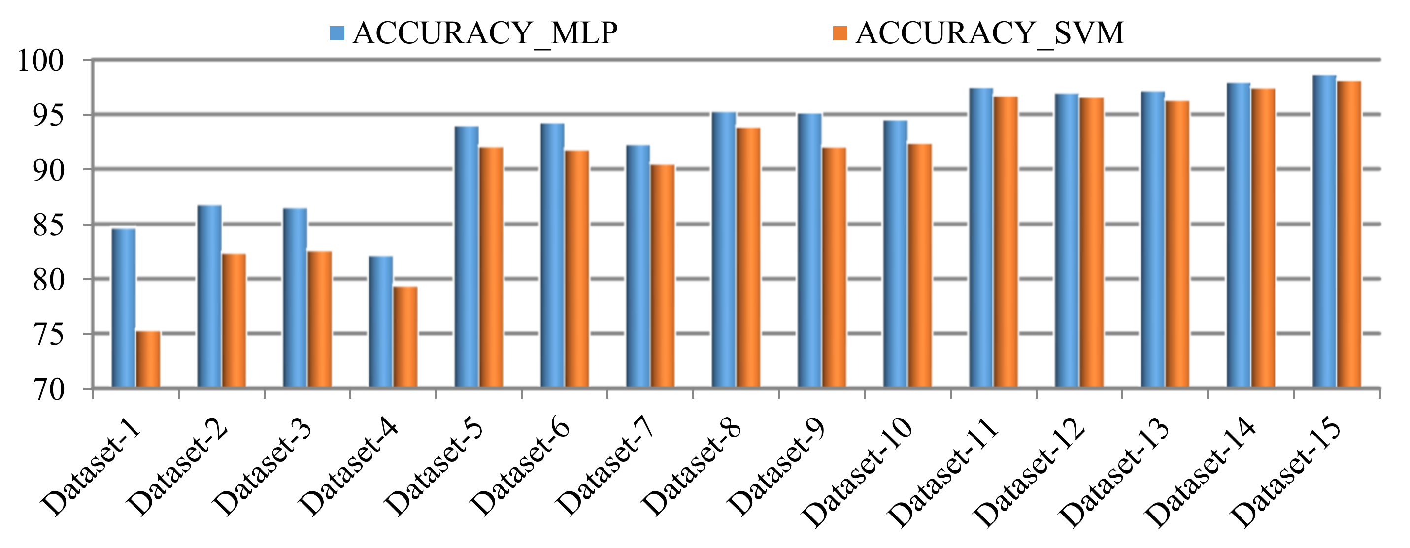
| 1 | D1 | 84.70 | 75.37 |
| 2 | D2 | 86.85 | 82.44 |
| 3 | D3 | 86.59 | 82.66 |
| 4 | D4 | 82.22 | 79.44 |
| 5 | D5 | 94.07 | 92.14 |
| 6 | D6 | 94.33 | 91.85 |
| 7 | D7 | 92.33 | 90.55 |
| 8 | D8 | 95.37 | 93.92 |
| 9 | D9 | 95.22 | 92.11 |
| 10 | D10 | 94.59 | 92.44 |
| 11 | D11 | 97.55 | 96.77 |
| 12 | D12 | 97.03 | 96.66 |
| 13 | D13 | 97.25 | 96.37 |
| 14 | D14 | 98.03 | 97.51 |
| 15 | D15 | 98.73 | 98.18 |
| Cls. No. | Dev. Char | D1 | D2 | D3 | D4 | D5 | D6 | D7 | D8 | D9 | D10 | D11 | D12 | D13 | D14 | D15 | Avg. |
|---|---|---|---|---|---|---|---|---|---|---|---|---|---|---|---|---|---|
| 0 | क | 0.93 | 0.97 | 0.90 | 0.83 | 0.97 | 0.97 | 0.96 | 0.99 | 0.96 | 1.00 | 1.00 | 0.97 | 1.00 | 0.99 | 1.00 | 0.96 |
| 1 | ख | 0.78 | 0.91 | 0.86 | 0.92 | 0.93 | 0.99 | 0.93 | 0.94 | 0.96 | 0.99 | 0.95 | 1.00 | 0.95 | 0.98 | 0.99 | 0.94 |
| 2 | ग | 0.88 | 0.87 | 0.85 | 0.96 | 0.92 | 0.99 | 0.88 | 0.97 | 0.97 | 0.97 | 0.97 | 1.00 | 0.99 | 1.00 | 0.99 | 0.95 |
| 3 | घ | 0.71 | 0.92 | 0.80 | 0.68 | 0.96 | 0.90 | 0.87 | 0.94 | 0.92 | 0.89 | 0.97 | 0.88 | 0.93 | 0.99 | 0.97 | 0.89 |
| 4 | ङ | 0.85 | 0.80 | 0.93 | 0.68 | 0.94 | 0.94 | 0.85 | 0.91 | 0.91 | 0.93 | 0.97 | 0.95 | 1.00 | 0.99 | 0.99 | 0.91 |
| 5 | च | 0.91 | 0.99 | 0.96 | 0.79 | 0.96 | 1.00 | 0.99 | 1.00 | 0.95 | 0.97 | 1.00 | 1.00 | 1.00 | 0.99 | 1.00 | 0.97 |
| 6 | छ | 0.90 | 0.83 | 0.85 | 0.90 | 0.99 | 0.94 | 0.95 | 0.96 | 0.98 | 0.91 | 0.98 | 0.98 | 0.96 | 1.00 | 0.99 | 0.94 |
| 7 | ज | 0.89 | 0.93 | 0.89 | 0.82 | 0.95 | 0.97 | 0.97 | 0.97 | 0.96 | 0.99 | 0.99 | 0.99 | 0.97 | 1.00 | 0.99 | 0.95 |
| 8 | झ | 0.96 | 0.95 | 0.96 | 0.89 | 0.95 | 0.99 | 0.95 | 0.97 | 1.00 | 0.97 | 1.00 | 1.00 | 0.98 | 1.00 | 1.00 | 0.97 |
| 9 | ञ | 0.91 | 0.91 | 0.94 | 0.89 | 0.96 | 0.94 | 0.96 | 0.98 | 1.00 | 0.98 | 0.96 | 0.99 | 0.99 | 1.00 | 0.99 | 0.96 |
| 10 | ट | 0.87 | 0.91 | 0.86 | 0.90 | 1.00 | 0.95 | 0.94 | 0.97 | 0.99 | 0.94 | 1.00 | 0.98 | 0.99 | 1.00 | 0.99 | 0.95 |
| 11 | ठ | 0.90 | 0.94 | 0.90 | 0.86 | 0.91 | 0.96 | 0.94 | 0.98 | 0.99 | 1.00 | 1.00 | 1.00 | 1.00 | 1.00 | 1.00 | 0.96 |
| 12 | ड | 0.87 | 0.84 | 0.87 | 0.78 | 0.93 | 0.89 | 0.91 | 0.96 | 0.99 | 0.94 | 0.97 | 0.94 | 0.97 | 0.99 | 0.99 | 0.92 |
| 13 | ढ | 0.85 | 0.78 | 0.89 | 0.90 | 0.94 | 0.93 | 0.95 | 0.94 | 0.94 | 0.94 | 0.97 | 0.97 | 0.99 | 0.93 | 0.99 | 0.93 |
| 14 | ण | 0.86 | 0.95 | 0.96 | 0.88 | 0.92 | 0.98 | 0.97 | 0.99 | 1.00 | 1.00 | 0.97 | 0.98 | 0.99 | 1.00 | 0.99 | 0.96 |
| 15 | त | 0.95 | 0.95 | 0.96 | 0.77 | 0.97 | 0.94 | 0.96 | 0.95 | 0.93 | 0.96 | 0.97 | 1.00 | 0.99 | 0.97 | 0.99 | 0.95 |
| 16 | थ | 0.90 | 0.84 | 0.84 | 0.74 | 0.97 | 0.93 | 0.94 | 0.95 | 0.94 | 0.90 | 1.00 | 0.96 | 0.97 | 0.98 | 0.98 | 0.92 |
| 17 | द | 0.91 | 0.85 | 0.82 | 0.75 | 0.85 | 0.95 | 0.89 | 0.96 | 0.87 | 0.85 | 0.92 | 0.94 | 0.94 | 0.95 | 0.98 | 0.90 |
| 18 | ध | 0.80 | 0.84 | 0.84 | 0.85 | 0.89 | 0.93 | 0.92 | 0.93 | 0.95 | 0.91 | 0.96 | 0.97 | 0.95 | 0.93 | 0.98 | 0.91 |
| 19 | न | 0.91 | 0.84 | 0.90 | 0.79 | 0.95 | 0.95 | 0.88 | 0.95 | 0.91 | 0.92 | 0.97 | 1.00 | 0.99 | 0.95 | 1.00 | 0.93 |
| 20 | प | 0.85 | 0.91 | 0.86 | 0.82 | 0.93 | 0.93 | 0.91 | 0.98 | 0.96 | 0.96 | 1.00 | 1.00 | 0.98 | 1.00 | 1.00 | 0.94 |
| 21 | फ | 0.90 | 0.94 | 0.92 | 0.81 | 0.99 | 0.99 | 0.95 | 0.98 | 0.97 | 0.99 | 1.00 | 0.99 | 0.98 | 0.96 | 1.00 | 0.96 |
| 22 | ब | 0.74 | 0.85 | 0.86 | 0.81 | 0.90 | 0.92 | 0.93 | 0.91 | 0.89 | 0.92 | 0.96 | 0.99 | 0.95 | 1.00 | 0.98 | 0.91 |
| 23 | भ | 0.82 | 0.78 | 0.79 | 0.76 | 0.89 | 0.93 | 0.92 | 0.90 | 0.90 | 0.91 | 1.00 | 0.97 | 0.97 | 0.99 | 0.98 | 0.90 |
| 24 | म | 0.81 | 0.83 | 0.81 | 0.86 | 0.91 | 0.96 | 0.91 | 0.93 | 0.95 | 0.98 | 0.96 | 0.94 | 0.94 | 0.97 | 0.99 | 0.92 |
| 25 | य | 0.80 | 0.87 | 0.83 | 0.83 | 0.89 | 0.92 | 0.93 | 0.90 | 0.92 | 0.88 | 0.92 | 0.94 | 0.93 | 0.96 | 0.96 | 0.90 |
| 26 | र | 0.90 | 0.88 | 0.89 | 0.72 | 0.96 | 0.93 | 0.95 | 0.99 | 0.99 | 0.98 | 0.99 | 0.99 | 1.00 | 1.00 | 0.99 | 0.94 |
| 27 | ल | 0.89 | 0.89 | 0.87 | 0.85 | 0.99 | 0.93 | 0.91 | 0.99 | 0.98 | 0.97 | 0.97 | 1.00 | 0.98 | 1.00 | 0.99 | 0.95 |
| 28 | व | 0.66 | 0.74 | 0.85 | 0.79 | 0.87 | 0.86 | 0.85 | 0.91 | 0.93 | 0.96 | 0.97 | 0.96 | 0.93 | 0.99 | 0.97 | 0.88 |
| 29 | श | 0.81 | 0.87 | 0.85 | 0.84 | 1.00 | 0.92 | 0.95 | 0.97 | 0.95 | 0.99 | 1.00 | 0.97 | 0.99 | 1.00 | 0.99 | 0.94 |
| 30 | ष | 0.81 | 0.85 | 0.87 | 0.84 | 0.99 | 0.96 | 0.90 | 0.97 | 1.00 | 0.93 | 0.99 | 0.98 | 0.99 | 0.99 | 0.99 | 0.94 |
| 31 | स | 0.80 | 0.76 | 0.76 | 0.81 | 0.95 | 0.90 | 0.88 | 0.92 | 0.93 | 0.94 | 1.00 | 0.92 | 0.96 | 0.99 | 0.98 | 0.90 |
| 32 | ह | 0.82 | 0.88 | 0.73 | 0.94 | 0.87 | 0.92 | 0.85 | 0.96 | 0.89 | 0.91 | 0.94 | 0.96 | 0.95 | 0.89 | 0.98 | 0.90 |
| 33 | क्ष | 0.77 | 0.82 | 0.88 | 0.77 | 0.97 | 0.95 | 0.89 | 0.92 | 0.99 | 0.92 | 0.99 | 0.89 | 0.97 | 0.95 | 0.99 | 0.91 |
| 34 | त्र | 0.75 | 0.82 | 0.86 | 0.88 | 0.95 | 0.97 | 0.92 | 0.95 | 0.98 | 0.97 | 1.00 | 0.99 | 0.99 | 0.99 | 0.99 | 0.93 |
| 35 | ज्ञ | 0.96 | 0.79 | 0.86 | 0.76 | 0.96 | 0.97 | 0.95 | 0.95 | 0.95 | 0.95 | 0.95 | 0.97 | 0.99 | 1.00 | 0.98 | 0.93 |
| Cls. No. | Dev.Char | D1 | D2 | D3 | D4 | D5 | D6 | D7 | D8 | D9 | D10 | D11 | D12 | D13 | D14 | D15 | Avg. |
|---|---|---|---|---|---|---|---|---|---|---|---|---|---|---|---|---|---|
| 0 | क | 0.89 | 0.90 | 0.93 | 0.74 | 0.97 | 0.96 | 0.95 | 0.99 | 0.99 | 0.97 | 1.00 | 1.00 | 0.98 | 0.96 | 1.00 | 0.95 |
| 1 | ख | 0.86 | 0.90 | 0.92 | 0.90 | 0.92 | 0.95 | 0.95 | 0.96 | 1.00 | 0.99 | 1.00 | 0.97 | 0.99 | 0.96 | 0.99 | 0.95 |
| 2 | ग | 0.83 | 0.87 | 0.91 | 0.84 | 0.97 | 0.94 | 0.98 | 0.98 | 0.99 | 0.98 | 0.99 | 0.94 | 0.99 | 1.00 | 0.99 | 0.95 |
| 3 | घ | 0.81 | 0.90 | 0.79 | 0.77 | 0.91 | 0.92 | 0.87 | 0.93 | 0.99 | 0.88 | 0.98 | 0.91 | 0.93 | 0.96 | 0.97 | 0.90 |
| 4 | ङ | 0.86 | 0.93 | 0.90 | 0.85 | 0.97 | 0.89 | 0.90 | 0.99 | 0.95 | 0.97 | 0.94 | 0.98 | 0.96 | 0.97 | 0.98 | 0.94 |
| 5 | च | 0.86 | 0.89 | 0.91 | 0.89 | 0.94 | 0.97 | 0.97 | 0.97 | 0.98 | 0.97 | 0.99 | 0.99 | 1.00 | 0.99 | 1.00 | 0.95 |
| 6 | छ | 0.87 | 0.83 | 0.91 | 0.85 | 0.95 | 0.94 | 0.95 | 0.97 | 0.95 | 0.84 | 0.95 | 0.95 | 0.96 | 0.95 | 0.98 | 0.92 |
| 7 | ज | 0.90 | 0.83 | 0.82 | 0.89 | 0.93 | 0.97 | 1.00 | 1.00 | 0.97 | 0.93 | 0.96 | 0.99 | 0.97 | 0.99 | 0.99 | 0.94 |
| 8 | झ | 0.97 | 0.96 | 0.96 | 0.88 | 0.98 | 0.99 | 0.97 | 0.95 | 0.97 | 0.99 | 1.00 | 0.99 | 1.00 | 1.00 | 1.00 | 0.97 |
| 9 | ञ | 0.89 | 0.93 | 0.83 | 0.85 | 0.94 | 0.97 | 0.91 | 0.95 | 0.94 | 0.97 | 0.99 | 0.96 | 0.99 | 0.99 | 0.99 | 0.94 |
| 10 | ट | 0.92 | 0.91 | 0.98 | 0.80 | 0.94 | 0.94 | 1.00 | 0.99 | 0.95 | 0.99 | 0.98 | 0.98 | 0.99 | 1.00 | 0.99 | 0.96 |
| 11 | ठ | 0.83 | 0.89 | 1.00 | 0.98 | 0.97 | 0.96 | 0.97 | 0.97 | 0.99 | 0.94 | 1.00 | 1.00 | 0.99 | 1.00 | 1.00 | 0.97 |
| 12 | ड | 0.86 | 0.93 | 0.80 | 0.89 | 0.88 | 0.97 | 0.88 | 0.93 | 0.97 | 0.93 | 1.00 | 1.00 | 0.98 | 0.98 | 0.98 | 0.93 |
| 13 | ढ | 0.90 | 0.87 | 0.86 | 0.80 | 0.95 | 0.93 | 0.92 | 0.97 | 0.95 | 0.94 | 0.96 | 1.00 | 0.97 | 0.96 | 0.99 | 0.93 |
| 14 | ण | 0.83 | 0.90 | 0.92 | 0.95 | 0.96 | 0.95 | 0.97 | 0.98 | 0.97 | 0.97 | 0.99 | 1.00 | 0.97 | 0.97 | 1.00 | 0.96 |
| 15 | त | 0.94 | 0.88 | 0.90 | 0.83 | 0.99 | 0.97 | 0.93 | 0.99 | 0.96 | 0.99 | 0.98 | 1.00 | 0.97 | 0.99 | 1.00 | 0.95 |
| 16 | थ | 0.85 | 0.86 | 0.82 | 0.75 | 0.89 | 0.96 | 0.94 | 0.95 | 0.93 | 0.88 | 0.98 | 0.99 | 0.93 | 0.98 | 0.98 | 0.91 |
| 17 | द | 0.85 | 0.74 | 0.85 | 0.69 | 0.95 | 0.95 | 0.87 | 0.97 | 0.96 | 0.92 | 0.96 | 0.93 | 0.97 | 0.93 | 0.98 | 0.90 |
| 18 | ध | 0.77 | 0.90 | 0.86 | 0.83 | 0.95 | 0.94 | 0.91 | 0.94 | 0.95 | 0.93 | 0.96 | 0.93 | 0.96 | 0.97 | 0.98 | 0.92 |
| 19 | न | 0.83 | 0.85 | 0.88 | 0.78 | 0.97 | 0.95 | 0.91 | 0.96 | 0.92 | 0.99 | 0.99 | 0.97 | 0.99 | 0.96 | 0.99 | 0.93 |
| 20 | प | 0.78 | 0.92 | 0.92 | 0.81 | 0.94 | 0.96 | 0.91 | 0.97 | 0.93 | 0.96 | 0.96 | 0.99 | 0.98 | 1.00 | 0.99 | 0.93 |
| 21 | फ | 0.87 | 0.96 | 0.86 | 0.83 | 0.99 | 0.97 | 0.97 | 0.98 | 0.99 | 0.96 | 0.97 | 1.00 | 0.99 | 1.00 | 1.00 | 0.96 |
| 22 | ब | 0.74 | 0.83 | 0.88 | 0.81 | 0.91 | 0.95 | 0.91 | 0.86 | 0.96 | 0.95 | 0.94 | 0.95 | 0.97 | 1.00 | 0.97 | 0.91 |
| 23 | भ | 0.76 | 0.82 | 0.76 | 0.81 | 0.94 | 0.88 | 0.95 | 0.91 | 0.95 | 0.97 | 0.95 | 0.92 | 0.93 | 0.97 | 0.98 | 0.90 |
| 24 | म | 0.84 | 0.82 | 0.90 | 0.88 | 0.94 | 0.93 | 0.89 | 0.88 | 0.91 | 0.96 | 0.95 | 1.00 | 0.98 | 1.00 | 0.98 | 0.92 |
| 25 | य | 0.78 | 0.83 | 0.83 | 0.77 | 0.87 | 0.89 | 0.86 | 0.94 | 0.92 | 0.92 | 0.99 | 0.99 | 0.98 | 1.00 | 0.97 | 0.90 |
| 26 | र | 0.85 | 0.84 | 0.81 | 0.83 | 0.92 | 0.94 | 0.95 | 1.00 | 0.96 | 1.00 | 0.99 | 0.97 | 0.94 | 0.99 | 0.99 | 0.93 |
| 27 | ल | 0.94 | 0.91 | 0.94 | 0.85 | 0.98 | 1.00 | 0.95 | 0.95 | 0.92 | 0.97 | 0.97 | 0.99 | 1.00 | 1.00 | 0.99 | 0.96 |
| 28 | व | 0.78 | 0.85 | 0.82 | 0.72 | 0.81 | 0.89 | 0.88 | 0.97 | 0.87 | 0.93 | 0.97 | 0.96 | 0.93 | 0.98 | 0.98 | 0.89 |
| 29 | श | 0.93 | 0.87 | 0.89 | 0.83 | 0.94 | 0.95 | 0.96 | 0.90 | 0.91 | 0.87 | 0.97 | 0.95 | 1.00 | 0.96 | 0.99 | 0.93 |
| 30 | ष | 0.85 | 0.86 | 0.87 | 0.82 | 0.97 | 0.95 | 0.93 | 0.95 | 0.95 | 0.97 | 0.97 | 0.99 | 0.97 | 0.99 | 0.99 | 0.94 |
| 31 | स | 0.75 | 0.75 | 0.76 | 0.83 | 0.92 | 0.91 | 0.84 | 0.93 | 0.91 | 0.88 | 0.99 | 0.95 | 0.93 | 0.97 | 0.98 | 0.89 |
| 32 | ह | 0.82 | 0.77 | 0.75 | 0.73 | 0.96 | 0.89 | 0.78 | 0.92 | 0.92 | 0.85 | 0.94 | 0.93 | 0.97 | 1.00 | 0.99 | 0.88 |
| 33 | क्ष | 0.87 | 0.86 | 0.87 | 0.80 | 0.93 | 0.94 | 0.88 | 0.93 | 0.96 | 0.96 | 1.00 | 0.97 | 0.97 | 1.00 | 0.98 | 0.93 |
| 34 | त्र | 0.83 | 0.82 | 0.85 | 0.79 | 0.94 | 0.95 | 0.94 | 0.95 | 0.98 | 0.97 | 0.97 | 0.95 | 1.00 | 0.99 | 0.98 | 0.93 |
| 35 | ज्ञ | 0.83 | 0.86 | 0.87 | 0.75 | 0.95 | 0.94 | 0.91 | 0.95 | 0.96 | 0.97 | 0.99 | 0.96 | 1.00 | 0.97 | 0.98 | 0.93 |
| Cls. No. | Dev.Char | D1 | D2 | D3 | D4 | D5 | D6 | D7 | D8 | D9 | D10 | D11 | D12 | D13 | D14 | D15 | Avg. |
|---|---|---|---|---|---|---|---|---|---|---|---|---|---|---|---|---|---|
| 0 | क | 0.91 | 0.94 | 0.92 | 0.78 | 0.97 | 0.96 | 0.95 | 0.99 | 0.98 | 0.98 | 1.00 | 0.98 | 0.99 | 0.98 | 1.00 | 0.96 |
| 1 | ख | 0.82 | 0.91 | 0.88 | 0.91 | 0.93 | 0.97 | 0.94 | 0.95 | 0.98 | 0.99 | 0.97 | 0.99 | 0.97 | 0.97 | 0.99 | 0.94 |
| 2 | ग | 0.85 | 0.87 | 0.88 | 0.90 | 0.94 | 0.96 | 0.93 | 0.98 | 0.98 | 0.98 | 0.98 | 0.97 | 0.99 | 1.00 | 0.99 | 0.95 |
| 3 | घ | 0.75 | 0.91 | 0.79 | 0.72 | 0.94 | 0.91 | 0.87 | 0.93 | 0.95 | 0.88 | 0.97 | 0.89 | 0.93 | 0.97 | 0.97 | 0.89 |
| 4 | ङ | 0.86 | 0.86 | 0.92 | 0.76 | 0.96 | 0.91 | 0.88 | 0.94 | 0.93 | 0.95 | 0.96 | 0.97 | 0.98 | 0.98 | 0.99 | 0.92 |
| 5 | च | 0.88 | 0.94 | 0.93 | 0.84 | 0.95 | 0.99 | 0.98 | 0.99 | 0.97 | 0.97 | 0.99 | 0.99 | 1.00 | 0.99 | 1.00 | 0.96 |
| 6 | छ | 0.89 | 0.83 | 0.88 | 0.87 | 0.97 | 0.94 | 0.95 | 0.97 | 0.97 | 0.87 | 0.97 | 0.97 | 0.96 | 0.98 | 0.98 | 0.93 |
| 7 | ज | 0.90 | 0.88 | 0.85 | 0.85 | 0.94 | 0.97 | 0.99 | 0.98 | 0.97 | 0.96 | 0.97 | 0.99 | 0.97 | 0.99 | 0.99 | 0.95 |
| 8 | झ | 0.97 | 0.95 | 0.96 | 0.88 | 0.96 | 0.99 | 0.96 | 0.96 | 0.99 | 0.98 | 1.00 | 0.99 | 0.99 | 1.00 | 1.00 | 0.97 |
| 9 | ञ | 0.90 | 0.92 | 0.88 | 0.87 | 0.95 | 0.96 | 0.93 | 0.96 | 0.97 | 0.97 | 0.97 | 0.97 | 0.99 | 0.99 | 0.99 | 0.95 |
| 10 | ट | 0.89 | 0.91 | 0.91 | 0.85 | 0.97 | 0.94 | 0.97 | 0.98 | 0.97 | 0.96 | 0.99 | 0.98 | 0.99 | 1.00 | 0.99 | 0.95 |
| 11 | ठ | 0.86 | 0.91 | 0.95 | 0.92 | 0.94 | 0.96 | 0.95 | 0.98 | 0.99 | 0.97 | 1.00 | 1.00 | 0.99 | 1.00 | 1.00 | 0.96 |
| 12 | ड | 0.86 | 0.88 | 0.83 | 0.83 | 0.90 | 0.93 | 0.90 | 0.95 | 0.98 | 0.94 | 0.98 | 0.97 | 0.97 | 0.98 | 0.98 | 0.93 |
| 13 | ढ | 0.87 | 0.82 | 0.88 | 0.85 | 0.95 | 0.93 | 0.93 | 0.95 | 0.94 | 0.94 | 0.97 | 0.98 | 0.98 | 0.95 | 0.99 | 0.93 |
| 14 | ण | 0.84 | 0.92 | 0.94 | 0.91 | 0.94 | 0.96 | 0.97 | 0.98 | 0.98 | 0.98 | 0.98 | 0.99 | 0.98 | 0.99 | 1.00 | 0.96 |
| 15 | त | 0.94 | 0.91 | 0.93 | 0.80 | 0.98 | 0.96 | 0.95 | 0.97 | 0.94 | 0.97 | 0.97 | 1.00 | 0.98 | 0.98 | 0.99 | 0.95 |
| 16 | थ | 0.88 | 0.85 | 0.83 | 0.74 | 0.93 | 0.95 | 0.94 | 0.95 | 0.93 | 0.89 | 0.99 | 0.97 | 0.95 | 0.98 | 0.98 | 0.92 |
| 17 | द | 0.88 | 0.79 | 0.84 | 0.72 | 0.90 | 0.95 | 0.88 | 0.97 | 0.92 | 0.88 | 0.94 | 0.93 | 0.96 | 0.94 | 0.98 | 0.90 |
| 18 | ध | 0.79 | 0.87 | 0.85 | 0.84 | 0.92 | 0.93 | 0.92 | 0.94 | 0.95 | 0.92 | 0.96 | 0.95 | 0.96 | 0.95 | 0.98 | 0.92 |
| 19 | न | 0.87 | 0.85 | 0.89 | 0.79 | 0.96 | 0.95 | 0.90 | 0.96 | 0.91 | 0.95 | 0.98 | 0.99 | 0.99 | 0.96 | 0.99 | 0.93 |
| 20 | प | 0.81 | 0.91 | 0.89 | 0.81 | 0.94 | 0.94 | 0.91 | 0.98 | 0.95 | 0.96 | 0.98 | 0.99 | 0.98 | 1.00 | 0.99 | 0.94 |
| 21 | फ | 0.89 | 0.95 | 0.89 | 0.82 | 0.99 | 0.98 | 0.96 | 0.98 | 0.98 | 0.98 | 0.98 | 0.99 | 0.98 | 0.98 | 1.00 | 0.96 |
| 22 | ब | 0.74 | 0.84 | 0.87 | 0.81 | 0.91 | 0.93 | 0.92 | 0.89 | 0.93 | 0.93 | 0.95 | 0.97 | 0.96 | 1.00 | 0.98 | 0.91 |
| 23 | भ | 0.79 | 0.80 | 0.77 | 0.78 | 0.91 | 0.91 | 0.93 | 0.90 | 0.92 | 0.94 | 0.98 | 0.95 | 0.95 | 0.98 | 0.98 | 0.90 |
| 24 | म | 0.83 | 0.82 | 0.85 | 0.87 | 0.93 | 0.94 | 0.90 | 0.90 | 0.93 | 0.97 | 0.96 | 0.97 | 0.96 | 0.99 | 0.98 | 0.92 |
| 25 | य | 0.79 | 0.85 | 0.83 | 0.80 | 0.88 | 0.91 | 0.90 | 0.92 | 0.92 | 0.90 | 0.95 | 0.96 | 0.95 | 0.98 | 0.96 | 0.90 |
| 26 | र | 0.87 | 0.86 | 0.85 | 0.77 | 0.94 | 0.94 | 0.95 | 0.99 | 0.97 | 0.99 | 0.99 | 0.98 | 0.97 | 0.99 | 0.99 | 0.94 |
| 27 | ल | 0.91 | 0.90 | 0.91 | 0.85 | 0.98 | 0.96 | 0.93 | 0.97 | 0.95 | 0.97 | 0.97 | 0.99 | 0.99 | 1.00 | 0.99 | 0.95 |
| 28 | व | 0.72 | 0.79 | 0.83 | 0.75 | 0.84 | 0.88 | 0.86 | 0.93 | 0.90 | 0.94 | 0.97 | 0.96 | 0.93 | 0.98 | 0.98 | 0.88 |
| 29 | श | 0.87 | 0.87 | 0.87 | 0.83 | 0.97 | 0.94 | 0.96 | 0.93 | 0.93 | 0.93 | 0.99 | 0.96 | 0.99 | 0.98 | 0.99 | 0.93 |
| 30 | ष | 0.83 | 0.86 | 0.87 | 0.83 | 0.98 | 0.95 | 0.92 | 0.96 | 0.98 | 0.95 | 0.98 | 0.98 | 0.98 | 0.99 | 0.99 | 0.94 |
| 31 | स | 0.77 | 0.75 | 0.76 | 0.82 | 0.93 | 0.91 | 0.86 | 0.93 | 0.92 | 0.91 | 0.99 | 0.93 | 0.94 | 0.98 | 0.98 | 0.89 |
| 32 | ह | 0.82 | 0.82 | 0.74 | 0.82 | 0.91 | 0.91 | 0.81 | 0.94 | 0.90 | 0.88 | 0.94 | 0.95 | 0.96 | 0.94 | 0.99 | 0.89 |
| 33 | क्ष | 0.82 | 0.84 | 0.88 | 0.79 | 0.95 | 0.94 | 0.88 | 0.93 | 0.97 | 0.94 | 0.99 | 0.93 | 0.97 | 0.97 | 0.98 | 0.92 |
| 34 | त्र | 0.79 | 0.82 | 0.85 | 0.83 | 0.95 | 0.96 | 0.93 | 0.95 | 0.98 | 0.97 | 0.99 | 0.97 | 0.99 | 0.99 | 0.99 | 0.93 |
| 35 | ज्ञ | 0.89 | 0.83 | 0.86 | 0.76 | 0.96 | 0.95 | 0.93 | 0.95 | 0.95 | 0.96 | 0.97 | 0.97 | 0.99 | 0.99 | 0.98 | 0.93 |
| Cls. No. | Dev.Char | D1 | D2 | D3 | D4 | D5 | D6 | D7 | D8 | D9 | D10 | D11 | D12 | D13 | D14 | D15 | Avg. |
|---|---|---|---|---|---|---|---|---|---|---|---|---|---|---|---|---|---|
| 0 | क | 0.84 | 0.87 | 0.89 | 0.76 | 0.97 | 0.91 | 0.96 | 0.98 | 0.91 | 0.98 | 0.99 | 0.97 | 1.00 | 1.00 | 1.00 | 0.94 |
| 1 | ख | 0.69 | 0.79 | 0.83 | 0.80 | 0.91 | 0.90 | 0.92 | 0.94 | 0.91 | 0.96 | 0.99 | 0.97 | 0.95 | 0.99 | 0.99 | 0.90 |
| 2 | ग | 0.77 | 0.85 | 0.79 | 0.88 | 0.85 | 0.94 | 0.94 | 0.98 | 0.97 | 0.98 | 0.97 | 0.99 | 0.98 | 0.94 | 0.98 | 0.92 |
| 3 | घ | 0.54 | 0.73 | 0.65 | 0.52 | 0.84 | 0.80 | 0.77 | 0.83 | 0.79 | 0.78 | 0.92 | 0.86 | 0.89 | 0.96 | 0.93 | 0.79 |
| 4 | ङ | 0.70 | 0.76 | 0.83 | 0.66 | 0.86 | 0.90 | 0.84 | 0.90 | 0.90 | 0.88 | 0.99 | 0.95 | 0.98 | 0.95 | 0.98 | 0.87 |
| 5 | च | 0.86 | 0.94 | 0.88 | 0.83 | 0.96 | 0.97 | 0.97 | 0.96 | 0.95 | 0.90 | 0.98 | 0.99 | 1.00 | 0.99 | 1.00 | 0.95 |
| 6 | छ | 0.84 | 0.75 | 0.79 | 0.82 | 0.93 | 0.94 | 0.91 | 0.92 | 0.93 | 0.84 | 0.93 | 0.95 | 0.93 | 0.99 | 0.96 | 0.90 |
| 7 | ज | 0.83 | 0.83 | 0.85 | 0.81 | 0.95 | 0.99 | 0.95 | 0.93 | 0.90 | 0.95 | 0.97 | 0.99 | 1.00 | 1.00 | 0.99 | 0.93 |
| 8 | झ | 0.90 | 0.93 | 0.89 | 0.93 | 0.98 | 0.96 | 0.95 | 0.98 | 0.99 | 0.97 | 0.99 | 0.98 | 0.98 | 0.99 | 0.99 | 0.96 |
| 9 | ञ | 0.87 | 0.85 | 0.81 | 0.81 | 0.94 | 0.96 | 0.97 | 0.96 | 0.99 | 0.86 | 0.99 | 0.99 | 0.99 | 0.99 | 0.99 | 0.93 |
| 10 | ट | 0.86 | 0.86 | 0.89 | 0.88 | 0.96 | 0.95 | 0.91 | 0.93 | 0.94 | 0.94 | 1.00 | 0.98 | 0.99 | 0.99 | 0.99 | 0.94 |
| 11 | ठ | 0.78 | 0.90 | 0.94 | 0.89 | 0.94 | 0.97 | 0.92 | 1.00 | 0.98 | 1.00 | 1.00 | 1.00 | 0.99 | 0.99 | 1.00 | 0.95 |
| 12 | ड | 0.78 | 0.73 | 0.82 | 0.84 | 0.97 | 0.90 | 0.91 | 0.91 | 0.96 | 0.91 | 0.95 | 0.97 | 0.97 | 0.98 | 0.98 | 0.91 |
| 13 | ढ | 0.81 | 0.76 | 0.86 | 0.81 | 0.93 | 0.92 | 0.95 | 0.96 | 0.90 | 0.93 | 0.91 | 0.97 | 0.93 | 0.93 | 0.97 | 0.90 |
| 14 | ण | 0.83 | 0.96 | 0.89 | 0.89 | 0.86 | 0.96 | 0.96 | 0.99 | 0.97 | 0.98 | 0.99 | 1.00 | 1.00 | 1.00 | 1.00 | 0.95 |
| 15 | त | 0.82 | 0.89 | 0.89 | 0.74 | 0.96 | 0.91 | 0.90 | 0.96 | 0.94 | 0.94 | 0.98 | 0.99 | 0.97 | 0.99 | 0.99 | 0.92 |
| 16 | थ | 0.66 | 0.73 | 0.79 | 0.72 | 0.98 | 0.90 | 0.86 | 0.90 | 0.83 | 0.91 | 0.99 | 0.97 | 0.93 | 0.95 | 0.97 | 0.87 |
| 17 | द | 0.66 | 0.80 | 0.70 | 0.79 | 0.88 | 0.89 | 0.84 | 0.90 | 0.79 | 0.90 | 0.96 | 0.94 | 0.96 | 0.99 | 0.97 | 0.86 |
| 18 | ध | 0.74 | 0.76 | 0.87 | 0.77 | 0.88 | 0.93 | 0.90 | 0.92 | 0.93 | 0.86 | 0.97 | 0.91 | 0.92 | 0.94 | 0.95 | 0.88 |
| 19 | न | 0.75 | 0.81 | 0.87 | 0.80 | 0.92 | 0.94 | 0.87 | 0.98 | 0.88 | 0.90 | 0.97 | 0.99 | 0.97 | 0.96 | 1.00 | 0.91 |
| 20 | प | 0.57 | 0.85 | 0.89 | 0.73 | 0.94 | 0.91 | 0.88 | 0.93 | 0.96 | 0.97 | 1.00 | 0.96 | 0.98 | 1.00 | 0.99 | 0.90 |
| 21 | फ | 0.88 | 0.97 | 0.92 | 0.85 | 0.99 | 0.97 | 0.95 | 0.98 | 0.96 | 0.97 | 1.00 | 1.00 | 0.98 | 0.98 | 1.00 | 0.96 |
| 22 | ब | 0.68 | 0.78 | 0.79 | 0.82 | 0.91 | 0.88 | 0.96 | 0.91 | 0.84 | 0.94 | 0.92 | 0.97 | 0.97 | 0.98 | 0.98 | 0.89 |
| 23 | भ | 0.62 | 0.66 | 0.67 | 0.73 | 0.85 | 0.85 | 0.80 | 0.87 | 0.88 | 0.83 | 0.93 | 0.93 | 0.95 | 0.95 | 0.96 | 0.83 |
| 24 | म | 0.77 | 0.71 | 0.87 | 0.94 | 0.84 | 0.87 | 0.91 | 0.88 | 1.00 | 0.93 | 0.94 | 0.96 | 0.89 | 0.97 | 0.98 | 0.90 |
| 25 | य | 0.63 | 0.81 | 0.82 | 0.77 | 0.92 | 0.89 | 0.93 | 0.97 | 0.85 | 0.86 | 0.89 | 0.95 | 0.92 | 0.94 | 0.94 | 0.87 |
| 26 | र | 0.82 | 0.86 | 0.97 | 0.82 | 0.98 | 0.95 | 0.94 | 0.97 | 0.96 | 0.98 | 1.00 | 0.99 | 0.99 | 0.99 | 0.99 | 0.95 |
| 27 | ल | 0.84 | 0.94 | 0.92 | 0.84 | 0.99 | 0.96 | 0.95 | 1.00 | 1.00 | 0.98 | 1.00 | 1.00 | 1.00 | 1.00 | 0.99 | 0.96 |
| 28 | व | 0.64 | 0.73 | 0.76 | 0.73 | 0.85 | 0.85 | 0.81 | 0.91 | 0.90 | 0.91 | 0.97 | 0.93 | 0.90 | 0.98 | 0.97 | 0.86 |
| 29 | श | 0.79 | 0.91 | 0.79 | 0.87 | 0.92 | 0.90 | 0.91 | 0.96 | 0.90 | 0.97 | 0.97 | 1.00 | 0.96 | 1.00 | 0.99 | 0.92 |
| 30 | ष | 0.69 | 0.86 | 0.86 | 0.89 | 0.96 | 0.96 | 0.96 | 0.95 | 0.98 | 0.92 | 0.99 | 1.00 | 0.98 | 1.00 | 0.99 | 0.93 |
| 31 | स | 0.70 | 0.75 | 0.74 | 0.69 | 0.88 | 0.89 | 0.85 | 0.88 | 0.88 | 0.93 | 0.97 | 0.95 | 0.95 | 0.94 | 0.97 | 0.86 |
| 32 | ह | 0.73 | 0.85 | 0.75 | 0.74 | 0.84 | 0.87 | 0.89 | 0.96 | 0.89 | 0.88 | 0.94 | 0.92 | 0.93 | 0.94 | 0.97 | 0.87 |
| 33 | क्ष | 0.80 | 0.86 | 0.78 | 0.78 | 0.97 | 0.92 | 0.85 | 0.93 | 0.93 | 0.93 | 1.00 | 0.96 | 1.00 | 0.99 | 0.99 | 0.91 |
| 34 | त्र | 0.72 | 0.87 | 0.78 | 0.83 | 0.93 | 0.95 | 0.90 | 0.95 | 0.98 | 0.97 | 0.99 | 0.99 | 0.99 | 0.97 | 0.99 | 0.92 |
| 35 | ज्ञ | 0.88 | 0.76 | 0.81 | 0.68 | 0.97 | 0.95 | 0.95 | 0.95 | 0.94 | 0.92 | 0.98 | 0.96 | 1.00 | 0.97 | 0.99 | 0.91 |
| Cls. No. | Dev.Char | D1 | D2 | D3 | D4 | D5 | D6 | D7 | D8 | D9 | D10 | D11 | D12 | D13 | D14 | D15 | Avg. |
|---|---|---|---|---|---|---|---|---|---|---|---|---|---|---|---|---|---|
| 0 | क | 0.88 | 0.90 | 0.89 | 0.82 | 1.00 | 0.94 | 0.99 | 0.96 | 0.97 | 0.95 | 0.99 | 0.98 | 0.98 | 0.98 | 1.00 | 0.95 |
| 1 | ख | 0.82 | 0.91 | 0.87 | 0.85 | 0.96 | 0.94 | 0.92 | 0.96 | 0.99 | 0.99 | 1.00 | 1.00 | 1.00 | 0.99 | 0.99 | 0.95 |
| 2 | ग | 0.79 | 0.89 | 0.84 | 0.86 | 0.99 | 0.93 | 0.97 | 1.00 | 0.95 | 0.95 | 0.99 | 0.99 | 1.00 | 1.00 | 0.99 | 0.94 |
| 3 | घ | 0.68 | 0.77 | 0.80 | 0.67 | 0.85 | 0.96 | 0.86 | 0.91 | 0.96 | 0.82 | 0.91 | 0.91 | 0.91 | 0.96 | 0.94 | 0.86 |
| 4 | ङ | 0.70 | 0.82 | 0.89 | 0.77 | 0.94 | 0.89 | 0.89 | 0.96 | 0.95 | 0.96 | 0.96 | 0.98 | 0.98 | 0.97 | 0.98 | 0.91 |
| 5 | च | 0.91 | 0.89 | 0.95 | 0.89 | 0.98 | 0.94 | 0.96 | 1.00 | 0.94 | 0.96 | 0.98 | 0.99 | 0.97 | 0.99 | 1.00 | 0.96 |
| 6 | छ | 0.70 | 0.78 | 0.81 | 0.80 | 0.92 | 0.91 | 0.97 | 0.99 | 0.94 | 0.86 | 0.95 | 0.94 | 0.94 | 0.95 | 0.97 | 0.90 |
| 7 | ज | 0.90 | 0.86 | 0.82 | 0.89 | 0.95 | 0.97 | 0.97 | 0.95 | 0.99 | 0.87 | 0.99 | 0.97 | 1.00 | 0.97 | 1.00 | 0.94 |
| 8 | झ | 0.86 | 0.94 | 0.93 | 0.90 | 0.95 | 0.97 | 0.96 | 1.00 | 0.97 | 0.99 | 1.00 | 1.00 | 1.00 | 1.00 | 1.00 | 0.96 |
| 9 | ञ | 0.78 | 0.93 | 0.89 | 0.86 | 0.96 | 0.97 | 0.93 | 0.91 | 0.93 | 0.93 | 0.99 | 0.97 | 0.99 | 0.99 | 0.99 | 0.93 |
| 10 | ट | 0.90 | 0.94 | 0.93 | 0.73 | 0.94 | 0.97 | 0.99 | 0.99 | 0.93 | 0.98 | 0.97 | 1.00 | 0.97 | 1.00 | 0.99 | 0.95 |
| 11 | ठ | 0.80 | 0.87 | 0.97 | 0.98 | 0.97 | 0.95 | 0.92 | 0.97 | 0.98 | 1.00 | 0.99 | 0.99 | 1.00 | 0.97 | 1.00 | 0.96 |
| 12 | ड | 0.81 | 0.83 | 0.81 | 0.83 | 0.86 | 0.88 | 0.91 | 0.92 | 0.94 | 0.89 | 0.98 | 1.00 | 0.98 | 0.99 | 0.99 | 0.91 |
| 13 | ढ | 0.82 | 0.78 | 0.81 | 0.76 | 0.92 | 0.93 | 0.90 | 0.93 | 0.89 | 0.90 | 0.95 | 0.97 | 0.97 | 0.99 | 0.98 | 0.90 |
| 14 | ण | 0.67 | 0.90 | 0.90 | 0.89 | 0.97 | 0.93 | 0.95 | 0.99 | 1.00 | 1.00 | 0.99 | 1.00 | 0.96 | 0.95 | 1.00 | 0.94 |
| 15 | त | 0.95 | 0.92 | 0.86 | 0.83 | 0.96 | 0.96 | 0.95 | 0.99 | 0.94 | 0.97 | 0.99 | 0.99 | 0.97 | 0.98 | 0.99 | 0.95 |
| 16 | थ | 0.76 | 0.77 | 0.75 | 0.73 | 0.94 | 0.89 | 0.92 | 0.92 | 0.84 | 0.85 | 0.98 | 0.96 | 0.91 | 0.98 | 0.96 | 0.88 |
| 17 | द | 0.82 | 0.76 | 0.76 | 0.72 | 0.91 | 0.88 | 0.90 | 0.92 | 0.84 | 0.88 | 0.91 | 0.89 | 0.90 | 0.91 | 0.95 | 0.86 |
| 18 | ध | 0.60 | 0.84 | 0.78 | 0.73 | 0.91 | 0.84 | 0.83 | 0.94 | 0.89 | 0.88 | 0.96 | 0.93 | 0.95 | 0.96 | 0.96 | 0.87 |
| 19 | न | 0.79 | 0.87 | 0.81 | 0.75 | 0.92 | 0.96 | 0.91 | 0.95 | 0.92 | 0.95 | 0.97 | 1.00 | 0.97 | 0.99 | 0.99 | 0.92 |
| 20 | प | 0.63 | 0.90 | 0.90 | 0.82 | 0.86 | 0.94 | 0.88 | 0.93 | 0.89 | 0.96 | 0.98 | 1.00 | 0.95 | 0.98 | 0.98 | 0.91 |
| 21 | फ | 0.86 | 0.91 | 0.86 | 0.88 | 0.99 | 0.97 | 0.97 | 1.00 | 0.96 | 0.95 | 1.00 | 0.99 | 1.00 | 1.00 | 0.99 | 0.96 |
| 22 | ब | 0.59 | 0.68 | 0.81 | 0.78 | 0.87 | 0.89 | 0.93 | 0.88 | 0.89 | 0.91 | 0.94 | 0.95 | 0.91 | 0.97 | 0.97 | 0.86 |
| 23 | भ | 0.72 | 0.74 | 0.68 | 0.74 | 0.88 | 0.86 | 0.89 | 0.93 | 0.87 | 0.92 | 0.98 | 0.95 | 0.94 | 0.97 | 0.97 | 0.87 |
| 24 | म | 0.72 | 0.69 | 0.82 | 0.87 | 0.87 | 0.86 | 0.87 | 0.84 | 0.94 | 0.94 | 0.95 | 0.96 | 0.98 | 0.96 | 0.98 | 0.88 |
| 25 | य | 0.51 | 0.76 | 0.78 | 0.69 | 0.81 | 0.86 | 0.87 | 0.87 | 0.86 | 0.88 | 0.95 | 0.96 | 0.98 | 1.00 | 0.96 | 0.85 |
| 26 | र | 0.69 | 0.83 | 0.90 | 0.87 | 0.91 | 0.94 | 0.95 | 1.00 | 0.97 | 0.99 | 1.00 | 0.96 | 0.97 | 1.00 | 0.99 | 0.93 |
| 27 | ल | 0.87 | 0.88 | 0.92 | 0.87 | 0.98 | 0.97 | 0.91 | 0.97 | 0.93 | 0.99 | 0.98 | 0.99 | 0.97 | 1.00 | 1.00 | 0.95 |
| 28 | व | 0.63 | 0.70 | 0.83 | 0.74 | 0.79 | 0.85 | 0.79 | 0.94 | 0.85 | 0.89 | 0.86 | 0.95 | 0.92 | 0.96 | 0.96 | 0.84 |
| 29 | श | 0.83 | 0.80 | 0.76 | 0.84 | 0.94 | 0.97 | 0.92 | 0.87 | 0.80 | 0.94 | 0.97 | 0.95 | 0.99 | 0.97 | 0.99 | 0.90 |
| 30 | ष | 0.68 | 0.81 | 0.83 | 0.79 | 0.92 | 0.88 | 0.90 | 0.95 | 0.94 | 0.95 | 0.96 | 0.95 | 0.93 | 0.99 | 0.99 | 0.90 |
| 31 | स | 0.59 | 0.70 | 0.66 | 0.71 | 0.89 | 0.84 | 0.75 | 0.88 | 0.87 | 0.87 | 0.97 | 0.96 | 0.94 | 0.93 | 0.97 | 0.84 |
| 32 | ह | 0.74 | 0.76 | 0.72 | 0.66 | 0.90 | 0.91 | 0.75 | 0.85 | 0.87 | 0.81 | 0.96 | 0.95 | 0.95 | 0.99 | 0.97 | 0.85 |
| 33 | क्ष | 0.83 | 0.72 | 0.87 | 0.67 | 0.93 | 0.91 | 0.84 | 0.92 | 0.87 | 0.91 | 0.99 | 0.97 | 0.96 | 0.96 | 0.99 | 0.89 |
| 34 | त्र | 0.64 | 0.79 | 0.80 | 0.83 | 0.93 | 0.91 | 0.92 | 0.93 | 0.98 | 0.94 | 0.97 | 0.92 | 0.97 | 0.97 | 0.99 | 0.90 |
| 35 | ज्ञ | 0.76 | 0.74 | 0.69 | 0.65 | 0.91 | 0.93 | 0.88 | 0.90 | 0.89 | 0.89 | 0.99 | 0.97 | 0.99 | 0.97 | 0.99 | 0.88 |
| Cls. No. | Dev.Char | D1 | D2 | D3 | D4 | D5 | D6 | D7 | D8 | D9 | D10 | D11 | D12 | D13 | D14 | D15 | Avg |
|---|---|---|---|---|---|---|---|---|---|---|---|---|---|---|---|---|---|
| 0 | क | 0.86 | 0.88 | 0.89 | 0.79 | 0.99 | 0.93 | 0.97 | 0.97 | 0.94 | 0.96 | 0.99 | 0.97 | 0.99 | 0.99 | 1.00 | 0.94 |
| 1 | ख | 0.75 | 0.85 | 0.85 | 0.82 | 0.94 | 0.92 | 0.92 | 0.95 | 0.95 | 0.97 | 0.99 | 0.99 | 0.98 | 0.99 | 0.99 | 0.92 |
| 2 | ग | 0.78 | 0.87 | 0.82 | 0.87 | 0.91 | 0.93 | 0.96 | 0.99 | 0.96 | 0.97 | 0.98 | 0.99 | 0.99 | 0.97 | 0.99 | 0.93 |
| 3 | घ | 0.60 | 0.75 | 0.72 | 0.58 | 0.84 | 0.87 | 0.81 | 0.87 | 0.86 | 0.80 | 0.92 | 0.88 | 0.90 | 0.96 | 0.94 | 0.82 |
| 4 | ङ | 0.70 | 0.79 | 0.86 | 0.71 | 0.89 | 0.89 | 0.86 | 0.93 | 0.92 | 0.92 | 0.97 | 0.97 | 0.98 | 0.96 | 0.98 | 0.89 |
| 5 | च | 0.89 | 0.91 | 0.91 | 0.86 | 0.97 | 0.96 | 0.97 | 0.98 | 0.95 | 0.93 | 0.98 | 0.99 | 0.98 | 0.99 | 1.00 | 0.95 |
| 6 | छ | 0.76 | 0.77 | 0.80 | 0.81 | 0.92 | 0.92 | 0.94 | 0.95 | 0.94 | 0.85 | 0.94 | 0.95 | 0.94 | 0.97 | 0.96 | 0.89 |
| 7 | ज | 0.87 | 0.84 | 0.84 | 0.85 | 0.95 | 0.98 | 0.96 | 0.94 | 0.94 | 0.90 | 0.98 | 0.98 | 1.00 | 0.99 | 0.99 | 0.93 |
| 8 | झ | 0.88 | 0.94 | 0.91 | 0.92 | 0.96 | 0.97 | 0.96 | 0.99 | 0.98 | 0.98 | 0.99 | 0.99 | 0.99 | 0.99 | 1.00 | 0.96 |
| 9 | ञ | 0.83 | 0.89 | 0.85 | 0.83 | 0.95 | 0.96 | 0.95 | 0.93 | 0.96 | 0.89 | 0.99 | 0.98 | 0.99 | 0.99 | 0.99 | 0.93 |
| 10 | ट | 0.88 | 0.90 | 0.91 | 0.80 | 0.95 | 0.96 | 0.95 | 0.96 | 0.93 | 0.96 | 0.98 | 0.99 | 0.98 | 0.99 | 0.99 | 0.94 |
| 11 | ठ | 0.79 | 0.89 | 0.95 | 0.93 | 0.95 | 0.96 | 0.92 | 0.98 | 0.98 | 1.00 | 0.99 | 0.99 | 0.99 | 0.98 | 1.00 | 0.95 |
| 12 | ड | 0.79 | 0.78 | 0.81 | 0.83 | 0.91 | 0.89 | 0.91 | 0.91 | 0.95 | 0.90 | 0.96 | 0.98 | 0.97 | 0.98 | 0.98 | 0.90 |
| 13 | ढ | 0.82 | 0.77 | 0.83 | 0.79 | 0.92 | 0.93 | 0.93 | 0.95 | 0.89 | 0.91 | 0.93 | 0.97 | 0.95 | 0.96 | 0.98 | 0.90 |
| 14 | ण | 0.74 | 0.93 | 0.90 | 0.89 | 0.91 | 0.95 | 0.96 | 0.99 | 0.98 | 0.99 | 0.99 | 1.00 | 0.98 | 0.97 | 1.00 | 0.95 |
| 15 | त | 0.88 | 0.91 | 0.87 | 0.78 | 0.96 | 0.94 | 0.92 | 0.98 | 0.94 | 0.96 | 0.98 | 0.99 | 0.97 | 0.98 | 0.99 | 0.94 |
| 16 | थ | 0.70 | 0.75 | 0.77 | 0.73 | 0.96 | 0.90 | 0.89 | 0.91 | 0.84 | 0.88 | 0.98 | 0.96 | 0.92 | 0.97 | 0.97 | 0.88 |
| 17 | द | 0.73 | 0.78 | 0.73 | 0.75 | 0.89 | 0.89 | 0.87 | 0.91 | 0.81 | 0.89 | 0.93 | 0.91 | 0.93 | 0.95 | 0.96 | 0.86 |
| 18 | ध | 0.67 | 0.80 | 0.82 | 0.75 | 0.90 | 0.88 | 0.86 | 0.93 | 0.91 | 0.87 | 0.97 | 0.92 | 0.94 | 0.95 | 0.96 | 0.88 |
| 19 | न | 0.77 | 0.84 | 0.84 | 0.77 | 0.92 | 0.95 | 0.89 | 0.96 | 0.90 | 0.92 | 0.97 | 0.99 | 0.97 | 0.98 | 0.99 | 0.91 |
| 20 | प | 0.60 | 0.88 | 0.90 | 0.78 | 0.90 | 0.92 | 0.88 | 0.93 | 0.92 | 0.97 | 0.99 | 0.98 | 0.96 | 0.99 | 0.99 | 0.91 |
| 21 | फ | 0.87 | 0.94 | 0.89 | 0.87 | 0.99 | 0.97 | 0.96 | 0.99 | 0.96 | 0.96 | 1.00 | 0.99 | 0.99 | 0.99 | 1.00 | 0.96 |
| 22 | ब | 0.63 | 0.72 | 0.80 | 0.80 | 0.89 | 0.89 | 0.95 | 0.90 | 0.86 | 0.92 | 0.93 | 0.96 | 0.94 | 0.98 | 0.97 | 0.88 |
| 23 | भ | 0.66 | 0.69 | 0.68 | 0.73 | 0.87 | 0.85 | 0.84 | 0.90 | 0.87 | 0.87 | 0.95 | 0.94 | 0.94 | 0.96 | 0.97 | 0.85 |
| 24 | म | 0.75 | 0.70 | 0.85 | 0.90 | 0.85 | 0.87 | 0.89 | 0.86 | 0.97 | 0.93 | 0.94 | 0.96 | 0.94 | 0.97 | 0.98 | 0.89 |
| 25 | य | 0.56 | 0.78 | 0.80 | 0.73 | 0.86 | 0.87 | 0.90 | 0.92 | 0.86 | 0.87 | 0.92 | 0.95 | 0.95 | 0.97 | 0.95 | 0.86 |
| 26 | र | 0.75 | 0.84 | 0.94 | 0.85 | 0.94 | 0.95 | 0.95 | 0.99 | 0.96 | 0.98 | 1.00 | 0.97 | 0.98 | 0.99 | 0.99 | 0.94 |
| 27 | ल | 0.86 | 0.91 | 0.92 | 0.85 | 0.98 | 0.96 | 0.93 | 0.99 | 0.96 | 0.98 | 0.99 | 0.99 | 0.98 | 1.00 | 1.00 | 0.95 |
| 28 | व | 0.63 | 0.72 | 0.80 | 0.73 | 0.82 | 0.85 | 0.80 | 0.93 | 0.88 | 0.90 | 0.91 | 0.94 | 0.91 | 0.97 | 0.97 | 0.85 |
| 29 | श | 0.81 | 0.85 | 0.77 | 0.85 | 0.93 | 0.93 | 0.92 | 0.91 | 0.85 | 0.95 | 0.97 | 0.97 | 0.97 | 0.99 | 0.99 | 0.91 |
| 30 | ष | 0.68 | 0.84 | 0.84 | 0.84 | 0.94 | 0.92 | 0.93 | 0.95 | 0.96 | 0.94 | 0.97 | 0.98 | 0.95 | 0.99 | 0.99 | 0.91 |
| 31 | स | 0.64 | 0.72 | 0.70 | 0.70 | 0.89 | 0.87 | 0.79 | 0.88 | 0.88 | 0.90 | 0.97 | 0.95 | 0.95 | 0.94 | 0.97 | 0.85 |
| 32 | ह | 0.74 | 0.81 | 0.74 | 0.70 | 0.87 | 0.89 | 0.81 | 0.90 | 0.88 | 0.84 | 0.95 | 0.94 | 0.94 | 0.96 | 0.97 | 0.86 |
| 33 | क्ष | 0.81 | 0.79 | 0.82 | 0.72 | 0.95 | 0.92 | 0.85 | 0.93 | 0.90 | 0.92 | 0.99 | 0.97 | 0.98 | 0.97 | 0.99 | 0.90 |
| 34 | त्र | 0.68 | 0.83 | 0.79 | 0.83 | 0.93 | 0.93 | 0.91 | 0.94 | 0.98 | 0.96 | 0.98 | 0.95 | 0.98 | 0.97 | 0.99 | 0.91 |
| 35 | ज्ञ | 0.81 | 0.75 | 0.75 | 0.67 | 0.94 | 0.94 | 0.91 | 0.92 | 0.92 | 0.90 | 0.98 | 0.97 | 0.99 | 0.97 | 0.99 | 0.89 |
| Sl. No. | Feature Type | Feature-Extraction Time (ms) | PCA Computation Time (ms) | Total Time (ms) |
|---|---|---|---|---|
| 1 | Bior-1.3 | 2.28 | 0.15 | 2.43 |
| 2 | VGG-19 | 0.10 | 0.69 | 0.79 |
| 3 | ResNet-50 | 0.08 | 0.40 | 0.48 |
| 4 | InceptionNet-V3 | 0.17 | 0.40 | 0.57 |
| Net time | 4.27 | |||
| Dataset Type | Mean Recognition-Time Per Character (Msec.) | |
|---|---|---|
| MLP Classifier | SVM Classifier | |
| Dataset 15 | 6.38 | 17.27 |
| Classifier | Characters |
|---|---|
| MLP | झ(Jha), ठ(Thha), च(Cha), ण(Adna), फ(Pha), क(Ka), ट(Taa), त(Ta), ल(La), ञ(Yna). |
| SVM | झ(Jha), फ(Pha), ठ(Thha), ल(La), च(Cha), ण(Adna), ट(Taa), क(Ka), र(Ra), त(Ta). |
| Classifier | Characters |
|---|---|
| MLP | थ(Tha), ध(Dha), ब(Ba), य(Ya), भ(Bha), द(Da), घ(Gha), स(Sa), ह(Ha), व(Wa). |
| SVM | ब(Ba), थ(Tha), ध(Dha), ह(Ha), द(Da), य(Ya), व(Wa), स(Sa), भ(Bha), घ(Gha). |
| Scheme 1. | Particular | Features Used | Classif. Scheme | No. of Test Samples | No. of Features for Classif. | Max. Recogn. Test-Acc. (%) | Data Set Used |
|---|---|---|---|---|---|---|---|
| 1 | Arora et al. 2008 [57] | Line fitting, intersection-points, shadow and chain code-based features | MLP | 1568 | 296 | 92.8 | [57] |
| 2 | Satish Kumar [58] | Gradient, neighborhood pixels weight, and distance transform-based features | SVM | 25,000 | 192 | 94.3 | [58] |
| 3 | Singh et al. 2011 [59] | Curvelet transform-based features | KNN | 7965 | 190 | 93.8 | [59] |
| 4 | Dixit et al. 2014 [27]. | Wavelet transform-based features | MLP | 600 | 256 | 70 | [27] |
| 5 | Jangid et al. 2014 [60] | Local auto-correlation of gradient | SVM | NA | 612 | 95.21 | [61] |
| 6 | Khanduja et al. 2015 [15]. | Hybrid of structural and statistical features | MLP | 4000 | 462 | 91.4 | [61] |
| 7 | Singh et al. 2015 [28]. | Chain code, zone-based centroid, background directional distribution and distance profile features | MLP and SVM | 4000 | 625 | 97.61 (SVM) | [28] |
| 8 | Jangid et al. 2016 [17]. | Fisher discriminant-based features | SVM | 10,850 | 256 | 96.58 | [62] |
| 9 | Sarkhel et al. 2017 [30]. | CNN-based features | SVM | 3894 | 4096, 2560 & 1792 | 95.180 | [63] |
| 10 | Nikita Singh, 2018 [16] | Histogram of gradients | MLP | 900 | 1224 | 97.5 | [16] |
| 11 | Gupta et al. 2019 [29] | HOG, convex hull, and longest run-based features | SVM | 10,800 | 5568 | 94.15 | [55] |
| 12 | Yadav et al. 2017 [64] | Projection profile-based features with HOG | Quadratic SVM | 4428 | NA | 96.6 | [62] |
| 13 | Proposed scheme | Hybrid of BDWT and DCNN-based features | MLP and SVM | 18,000 | 160 | 98.73 (MLP) | [55] |
Publisher’s Note: MDPI stays neutral with regard to jurisdictional claims in published maps and institutional affiliations. |
© 2021 by the authors. Licensee MDPI, Basel, Switzerland. This article is an open access article distributed under the terms and conditions of the Creative Commons Attribution (CC BY) license (https://creativecommons.org/licenses/by/4.0/).
Share and Cite
Rajpal, D.; Garg, A.R.; Mahela, O.P.; Alhelou, H.H.; Siano, P. A Fusion-Based Hybrid-Feature Approach for Recognition of Unconstrained Offline Handwritten Hindi Characters. Future Internet 2021, 13, 239. https://0-doi-org.brum.beds.ac.uk/10.3390/fi13090239
Rajpal D, Garg AR, Mahela OP, Alhelou HH, Siano P. A Fusion-Based Hybrid-Feature Approach for Recognition of Unconstrained Offline Handwritten Hindi Characters. Future Internet. 2021; 13(9):239. https://0-doi-org.brum.beds.ac.uk/10.3390/fi13090239
Chicago/Turabian StyleRajpal, Danveer, Akhil Ranjan Garg, Om Prakash Mahela, Hassan Haes Alhelou, and Pierluigi Siano. 2021. "A Fusion-Based Hybrid-Feature Approach for Recognition of Unconstrained Offline Handwritten Hindi Characters" Future Internet 13, no. 9: 239. https://0-doi-org.brum.beds.ac.uk/10.3390/fi13090239