
Solar Radiation Forecasting by Pearson Correlation Using LSTM Neural Network and ANFIS Method: Application in the West-Central Jordan


 ,
,  , and
, and
Abstract
:
1. Introduction
Related Work
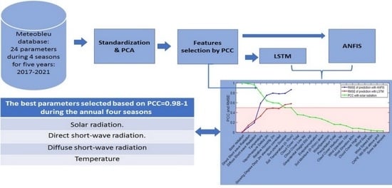
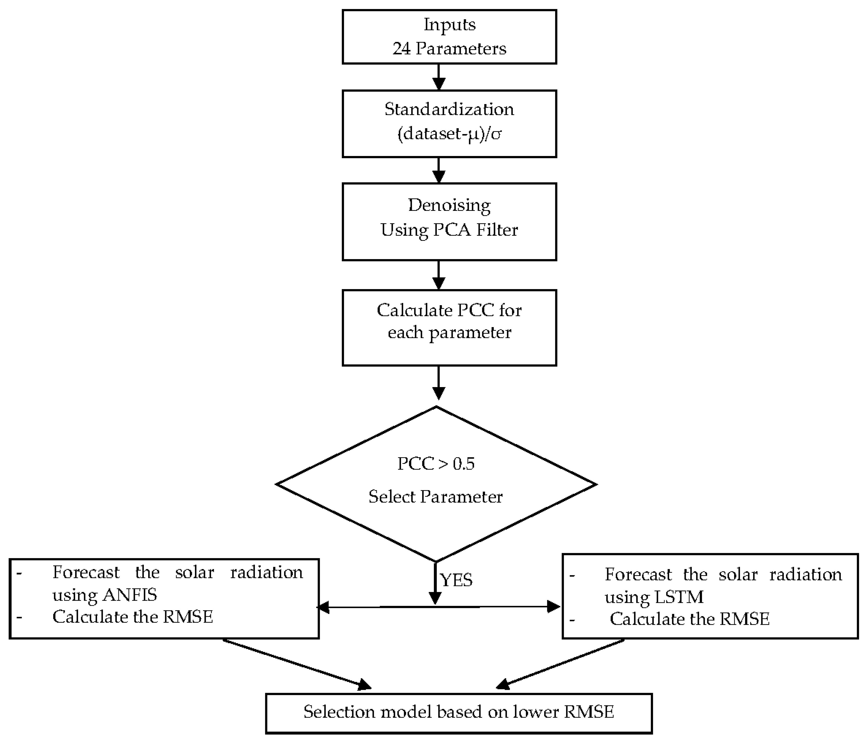
2. Materials and Methods
2.1. Data Standardization
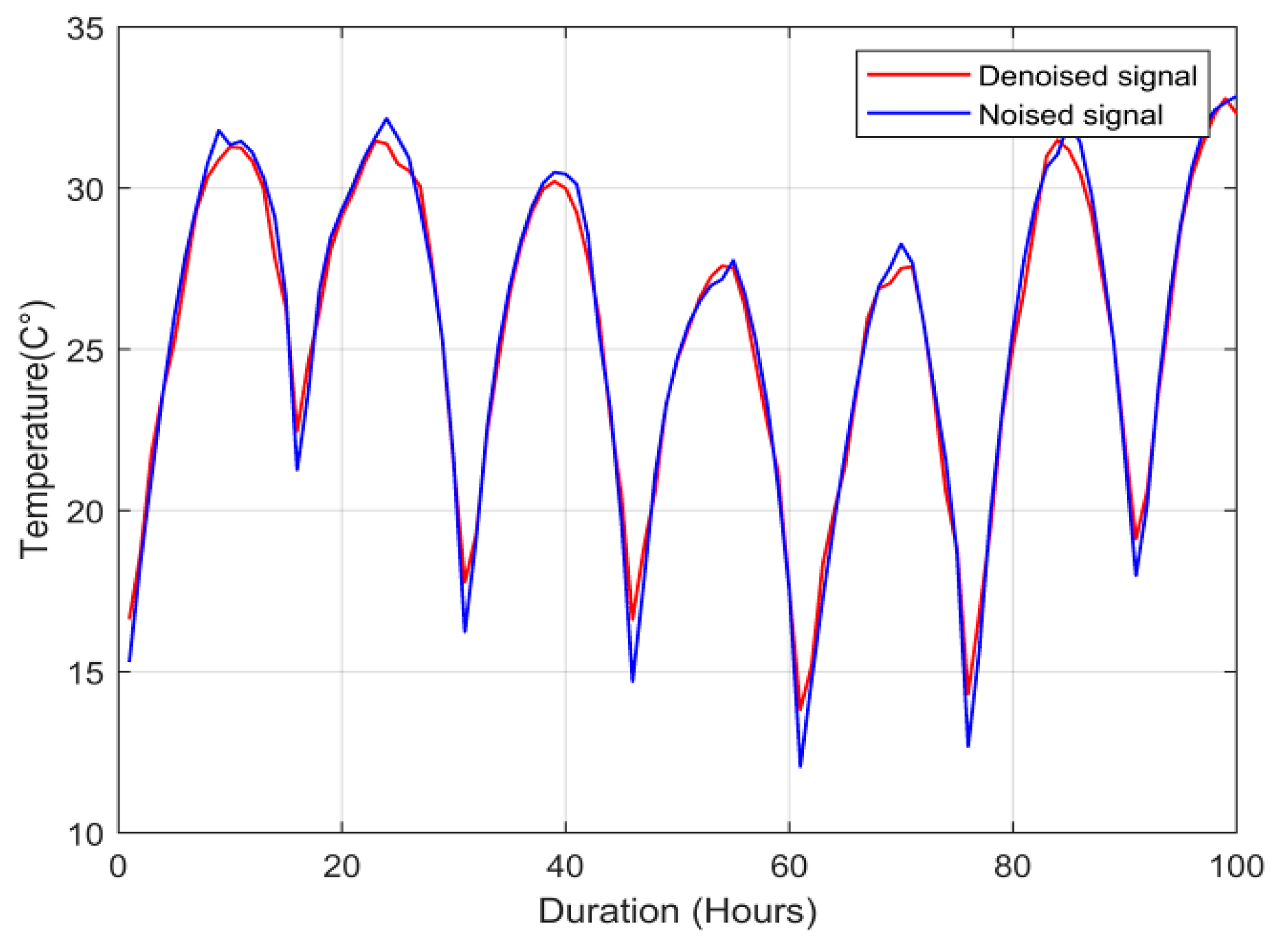
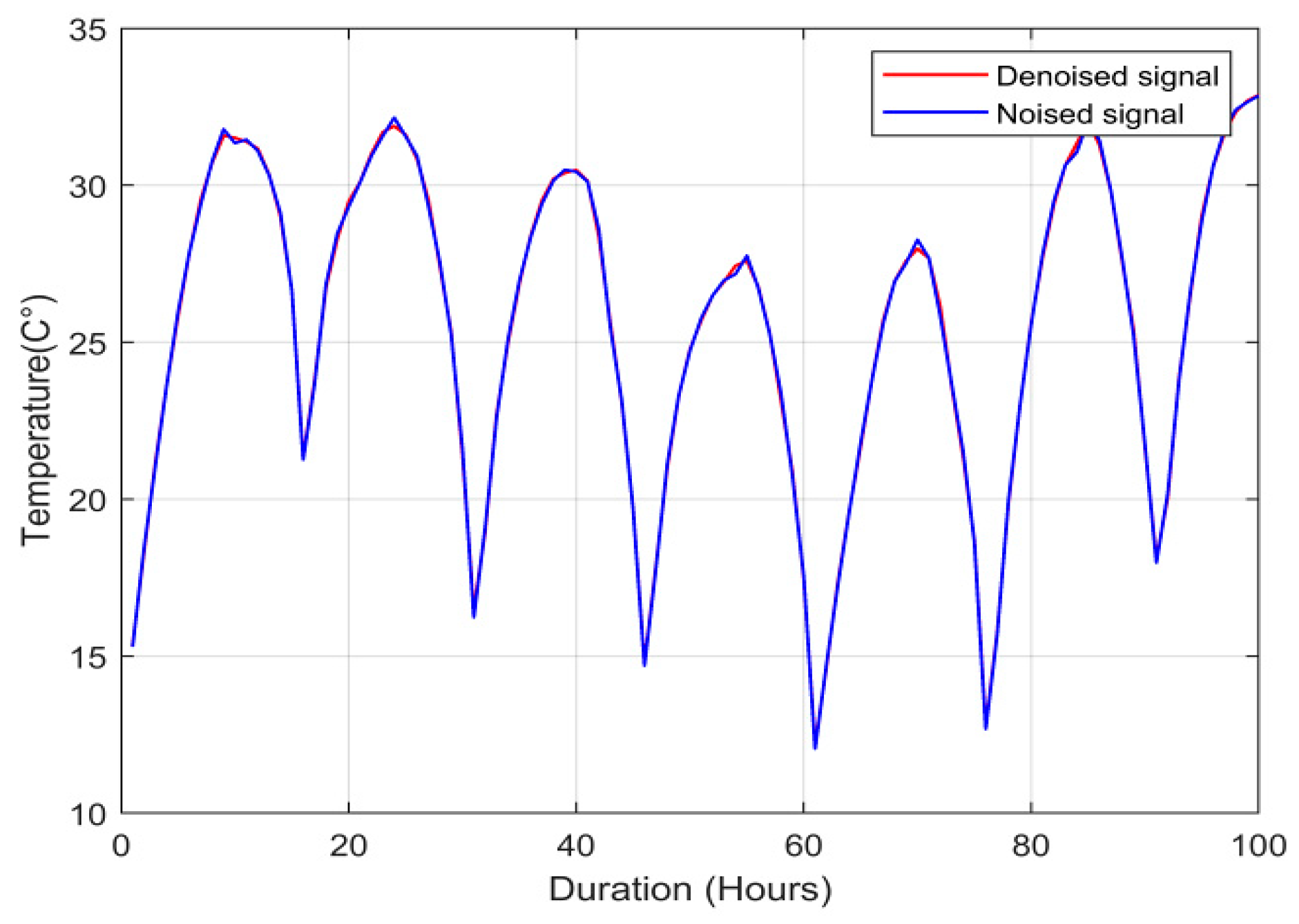
2.2. Principal Component Analysis (PCA) for Noise Filtering
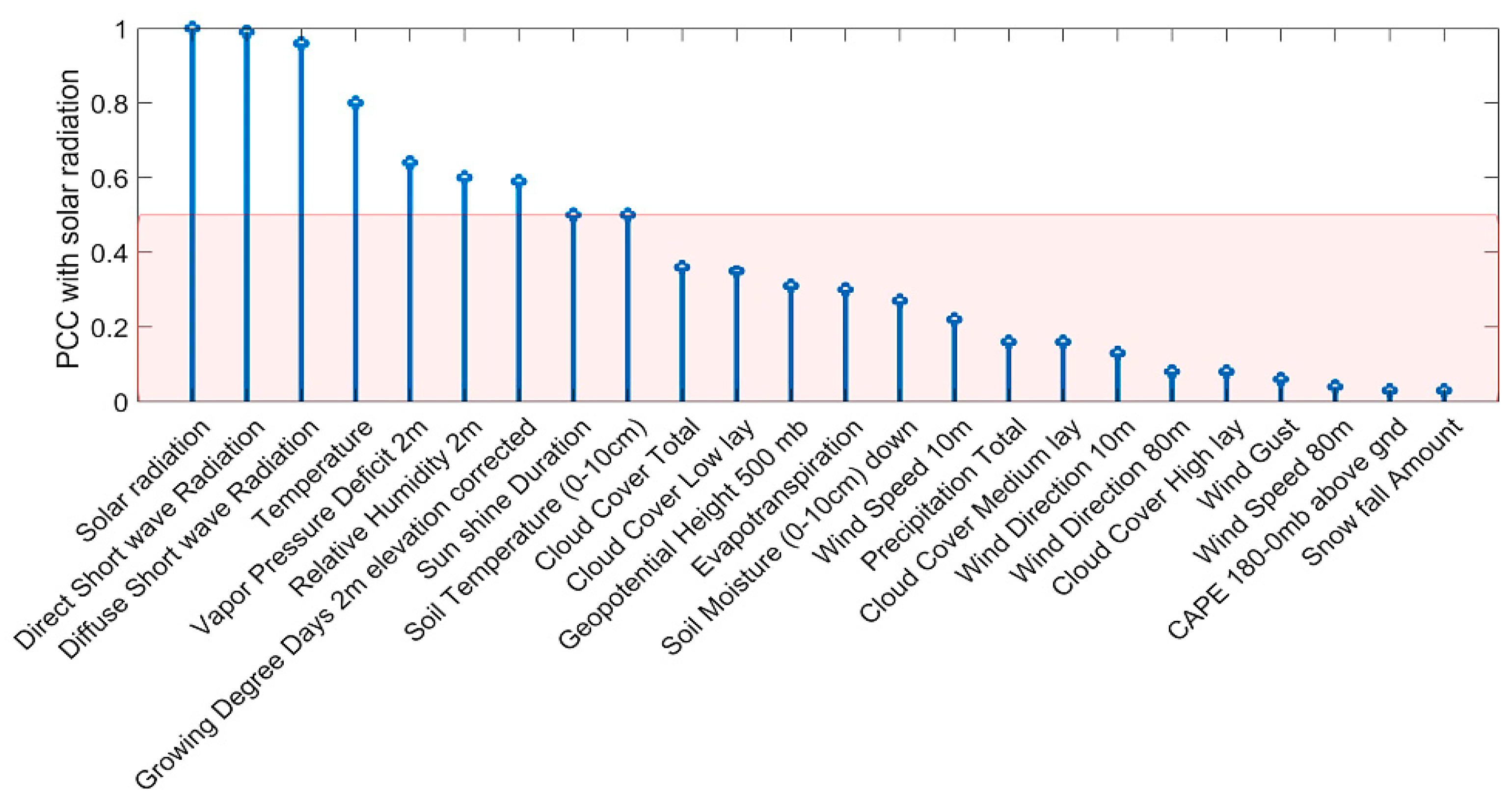
2.3. Feature Selection
2.4. Evaluation Measures
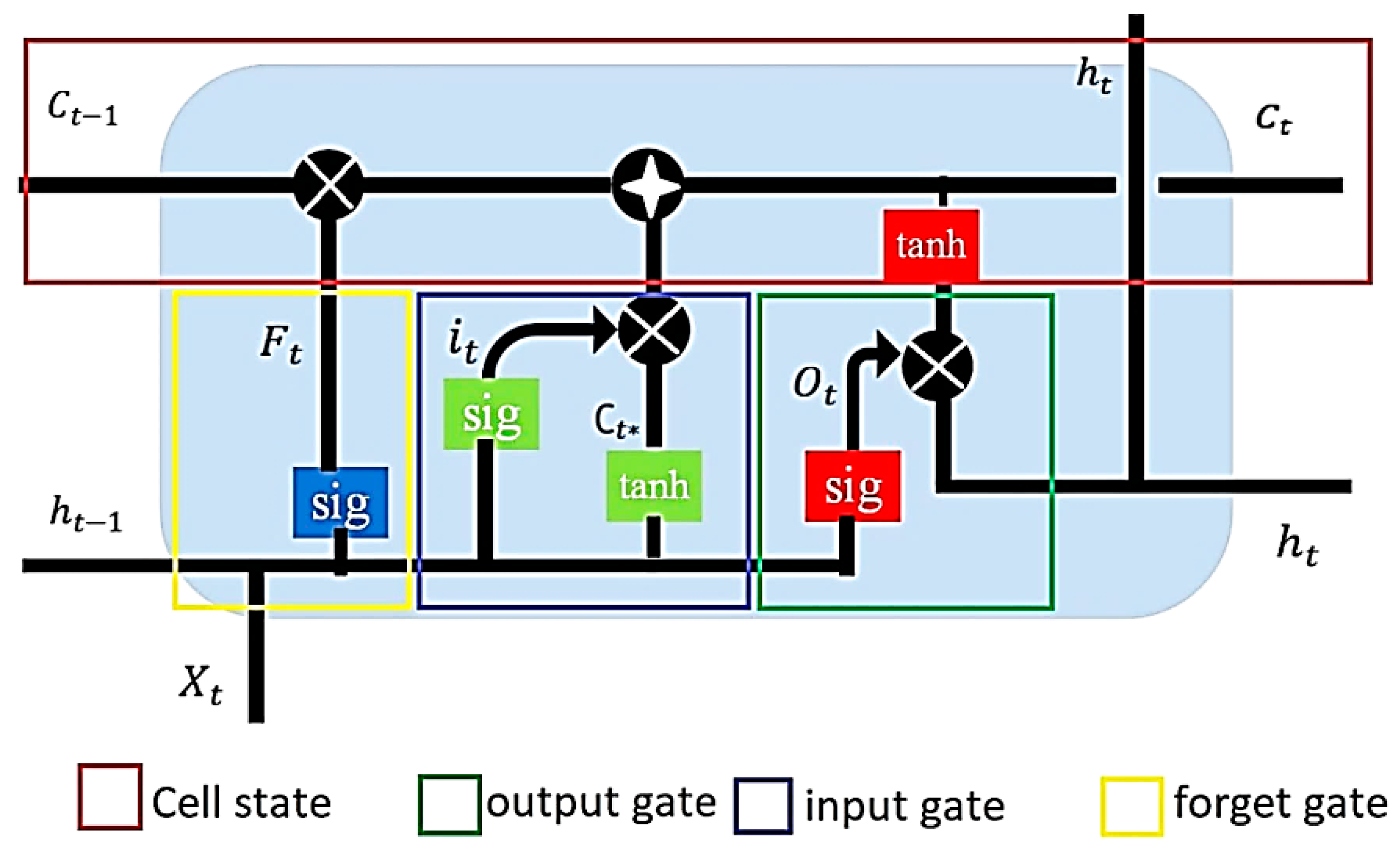
2.5. Long Short-Term Memory (LSTM) Network
- -
- Forget gate: its function is to decide whether to keep or forget the information. Only information from previously hidden layers and current input remain with the sigmoid function. Any value closer to one will remain, while values closer to zero will disappear:where is the input vector, are the output of the previous block, W and U the weight matrices of the hidden state and input respectively for each gate, is the sigmoid activation function.
- -
- Input Gate: the front door helps to update the cell condition. Current input and previous state information go through the sigmoid function, which updates the value by multiplying it by zero and one. Likewise, for network regulation, data also pass through the tanh function (Equation (9)); is the input gate vector.The cell state vector aggregates the two components (old memory via the forget gate and new memory via the input gate)is a memory from the previous block, is defined as a memory from the current block; the “∗” operator is the Hadamard product.
- -
- Output Gate: the next hidden state is set in the output gate. The sigmoid output has to be multiplied by the tanh function; the result of this multiplication decides which information the hidden state h_t should carry. This hidden state is used for the prediction. After, the new hidden state and cell state will move on to the next step:where is the output gate vector, and the current block output. Table 2 illustrates the used training hyper-parameters for the LSTM neural network.
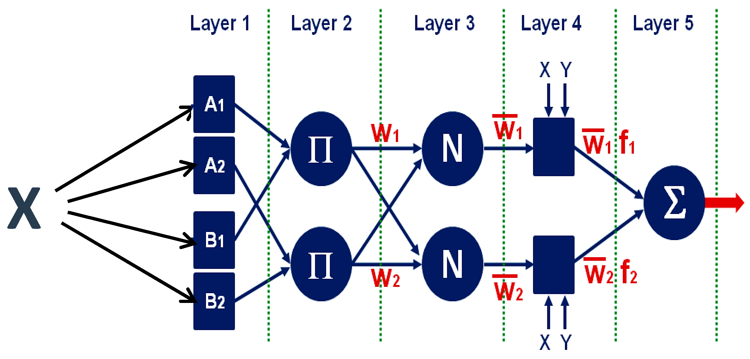
2.6. Adaptive Neuro-Fuzzy Inference System (ANFIS)
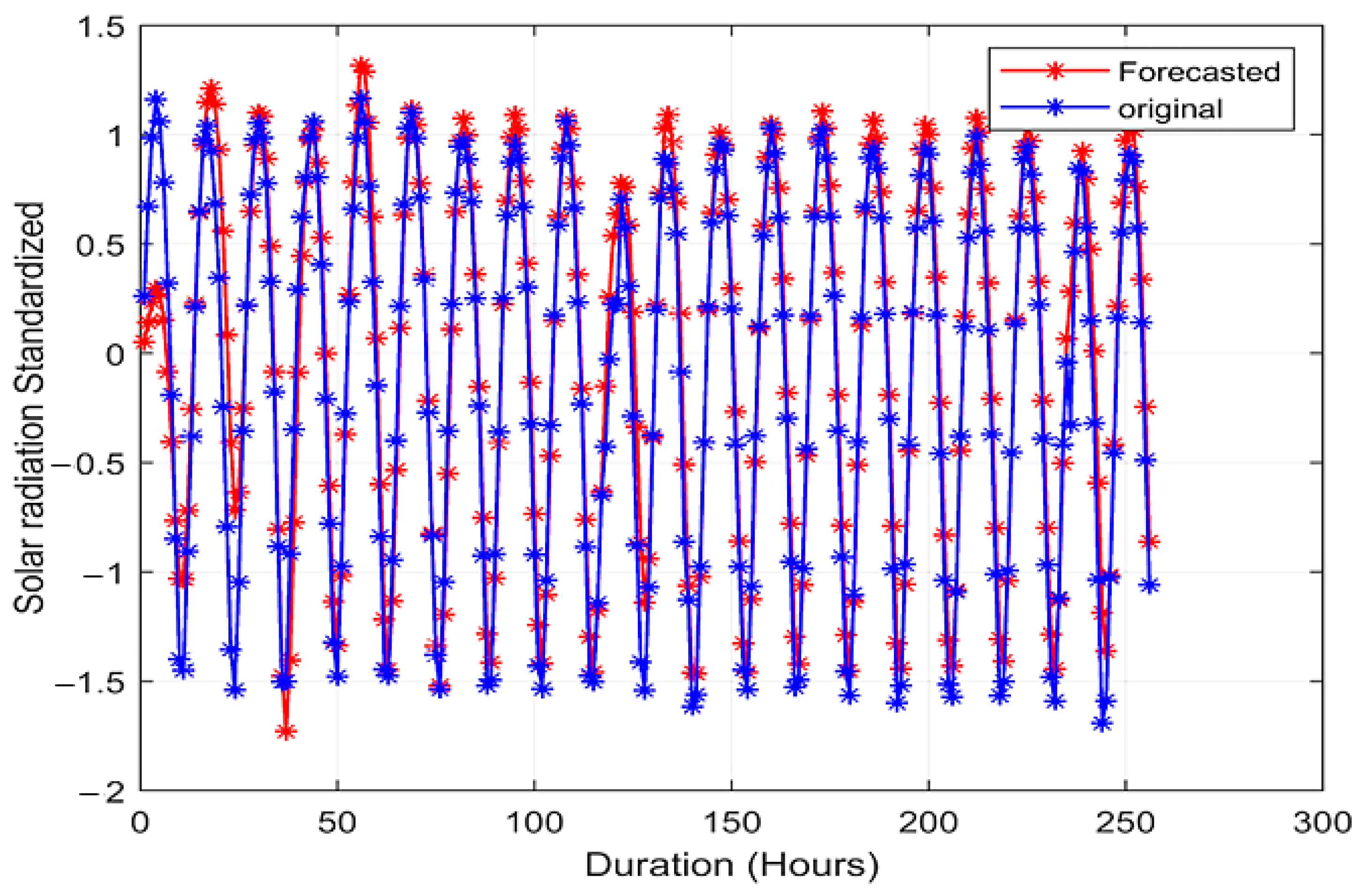
3. Results
4. Discussion
5. Conclusions
Author Contributions
Funding
Institutional Review Board Statement
Informed Consent Statement
Data Availability Statement
Conflicts of Interest
Abbreviations
| Acronyms | Extended Meaning of the Acronym |
| LSTM | Long short-term memory |
| ANFIS | Adaptive neuro fuzzy inference system |
| PCC | Pearson correlation coefficient |
| PCA | Principal Component Analysis |
| PV | Photovoltaic |
| ML | Machine learning |
| DL | Deep learning |
| GDP | Gross Domestic Product |
| VPD | Vapor pressure deficit |
| CAPE | Convective available potential energy |
| RMSE | Root-Mean-Square Error |
| SVM | Support Vector Machines |
| RF | Random Forest |
| CNN | Convolutional Neural Network |
| ARTS | Auto-regressive time-series |
| ANN | Artificial Neural Network |
| MAE | Mean Absolute Error |
| NNM | Neural network models |
| SVD | Singular value decomposition |
| NIPALS | Nonlinear iterative partial least squares |
| SAO | Successive average orthogonalization |
| MLP | Multilayer perceptron |
| RNN | Recurrent neural network |
| GRU | Gated recurrent unit |
| ARX | Autoregressive-exogenous |
| LR | Linear regression |
References
- Sayed, E.T.; Wilberforce, T.; Elsaid, K.; Rabaia, M.K.H.; Abdelkareem, M.A.; Chae, K.-J.; Olabi, A.G. A critical review on environmental impacts of renewable energy systems and mitigation strategies: Wind, hydro, biomass and geothermal. Sci. Total Environ. 2021, 766, 144505. [Google Scholar] [CrossRef] [PubMed]
- de Araujo, J.M.S. Improvement of Coding for Solar Radiation Forecasting in Dili Timor Leste—A WRF Case Study. J. Power Energy Eng. 2021, 9, 7–20. [Google Scholar] [CrossRef]
- Ziane, A.; Necaibia, A.; Sahouane, N.; Dabou, R.; Mostefaoui, M.; Bouraiou, A.; Khelifi, S.; Rouabhia, A.; Blal, M. Photovoltaic output power performance assessment and forecasting: Impact of meteorological variables. Sol. Energy 2021, 220, 745–757. [Google Scholar] [CrossRef]
- Alawasa, K.M.; Al-Odienat, A.I. Power quality characteristics of residential grid-connected inverter ofphotovoltaic solar system. In Proceedings of the 2017 IEEE 6th International Conference on Renewable Energy Research and Applications (ICRERA), San Diego, CA, USA, 5–8 November 2017; pp. 1097–1101. [Google Scholar] [CrossRef]
- Gielen, D.; Boshell, F.; Saygin, D.; Bazilian, M.D.; Wagner, N.; Gorini, R. The role of renewable energy in the global energy transformation. Energy Strategy Rev. 2019, 24, 38–50. [Google Scholar] [CrossRef]
- Strielkowski, W.; Civin, L.; Tarkhanova, E.; Tvaronaviciene, M.; Petrenko, Y. Renewable Energy in the Sustainable Development of Electrical Power Sector: A Review unit. Energies 2021, 14, 8240. [Google Scholar] [CrossRef]
- Lay-Ekuakille, A.; Ciaccioli, A.; Griffo, G.; Visconti, P.; Andria, G. Effects of Dust on Photovoltaic Measurements: A Comparative Study. Measurement 2018, 113, 181–188. [Google Scholar] [CrossRef]
- McGee, T.G.; Mori, K. The Management of Urbanization, Development, and Environmental Change in the Megacities of Asia in the Twenty-First Century. In Living in the Megacity: Towards Sustainable Urban Environments; Springer: Tokyo, Japan, 2021; Volume 17, Chapter 2; ISBN 978-4-431-56899-5. [Google Scholar] [CrossRef]
- Wilson, G.A.; Bryant, R.L. Environmental Management: New Directions for the Twenty-First Century; Routledge: London, UK, 2021; ISBN 9780203974988. [Google Scholar] [CrossRef]
- Ismail, A.M.; Ramirez-Iniguez, R.; Asif, M.; Munir, A.B.; Muhammad-Sukki, F. Progress of solar photovoltaic in ASEAN countries: A review. Renew. Sustain. Energy Rev. 2015, 48, 399–412. [Google Scholar] [CrossRef]
- Al-Odienat, A.; Al-Maitah, K. A modified Active Frequency Drift Method for Islanding Detection. In Proceedings of the 2021 12th International Renewable Engineering Conference (IREC), Amman, Jordan, 14–15 April 2021; pp. 1–6. [Google Scholar] [CrossRef]
- Srivastava, R.; Tiwari, A.N.; Giri, V.K. Prediction of Electricity Generation using Solar Radiation Forecasting Data. In Proceedings of the 2020 International Conference on Electrical and Electronics Engineering (ICE3), Gorakhpur, India, 14–15 February 2020. [Google Scholar] [CrossRef]
- Alawasa, K.M.; Al-Odienat, A.I. Power Quality Investigation of Single Phase Grid-connected Inverter of Photovoltaic System. J. Eng. Technol. Sci. 2019, 51, 597–614. [Google Scholar] [CrossRef]
- Castangia, M.; Aliberti, A.; Bottaccioli, L.; Macii, E.; Patti, E. A compound of feature selection techniques to improve solar radiation forecasting. Expert Syst. Appl. 2021, 178, 114979. [Google Scholar] [CrossRef]
- Prado-Rujas, I.I.; García-Dopico, A.; Serrano, E.; Pérez, M.S. A Flexible and Robust Deep Learning-Based System for Solar Irradiance Forecasting. IEEE Access 2021, 9, 12348–12361. [Google Scholar] [CrossRef]
- Yan, K.; Shen, H.; Wang, L.; Zhou, H.; Xu, M.; Mo, Y. Short-term solar irradiance forecasting based on a hybrid deep learning methodology. Information 2020, 11, 32. [Google Scholar] [CrossRef] [Green Version]
- Yen, C.F.; Hsieh, H.-Y.; Su, K.-W.; Yu, M.-C.; Leu, J.-S. Solar Power Prediction via Support Vector Machine and Random Forest. E3S Web Conf. 2018, 69, 01004. [Google Scholar] [CrossRef] [Green Version]
- Lee, W.; Kim, K.; Park, J.; Kim, J.; Kim, Y. Forecasting solar power using long-short term memory and convolutional neural networks. IEEE Access 2018, 6, 73068–73080. [Google Scholar] [CrossRef]
- Poolla, C.; Ishihara, A.K. Localized solar power prediction based on weather data from local history and global forecasts. In Proceedings of the 2018 IEEE 7th World Conference on Photovoltaic Energy Conversion (WCPEC) (A Joint Conference of 45th IEEE PVSC, 28th PVSEC, 34th EU PVSEC), Waikoloa, HI, USA, 10–15 June 2018; pp. 2341–2345. [Google Scholar] [CrossRef] [Green Version]
- Han, J.; Park, W.-K. A Solar Radiation Prediction Model Using Weather Forecast Data and Regional Atmospheric Data. In Proceedings of the 2018 IEEE 7th World Conference on Photovoltaic Energy Conversion (WCPEC) (A Joint Conference of 45th IEEE PVSC, 28th PVSEC & 34th EU PVSEC), Waikoloa, HI, USA, 10–15 June 2018; pp. 2313–2316. [Google Scholar] [CrossRef]
- Wang, Y.; Chen, Y.; Liu, H.; Ma, X.; Su, X.; Liu, Q. Day-Ahead Photovoltaic Power Forcasting Using Convolutional-LSTM Networks. In Proceedings of the 3rd Asia Energy and Electrical Engineering Symposium (AEEES), Chengdu, China, 26–29 March 2021; pp. 917–921. [Google Scholar] [CrossRef]
- Munir, M.A.; Khattak, A.; Imran, K.; Ulasyar, A.; Khan, A. Solar PV Generation Forecast Model Based on the Most Effective Weather Parameters. In Proceedings of the 2019 International Conference on Electrical, Communication, and Computer Engineering (ICECCE), Swat, Pakistan, 24–25 July 2019; pp. 1–5. [Google Scholar] [CrossRef]
- Obiora, C.N.; Ali, A.; Hasan, A.N. Estimation of Hourly Global Solar Radiation Using Deep Learning Algorithms. In Proceedings of the 2020 11th International Renewable Energy Congress (IREC), Hammamet, Tunisia, 29–31 October 2020; pp. 1–6. [Google Scholar] [CrossRef]
- de Guia, J.D.; Concepcion, R.S.; Calinao, H.A.; Alejandrino, J.; Dadios, E.P.; Sybingco, E. Using Stacked Long Short Term Memory with Principal Component Analysis for Short Term Prediction of Solar Irradiance based on Weather Patterns. In Proceedings of the 2020 IEEE Region 10 Conference (TENCON), Osaka, Japan, 16–19 November 2020. [Google Scholar] [CrossRef]
- Zou, M.; Fang, D.; Harrison, G.; Djokic, S. Weather Based Day-Ahead and Week-Ahead Load Forecasting using Deep Recurrent Neural Network. In Proceedings of the 2019 IEEE 5th International Forum on Research and Technology for Society and Industry (RTSI), Florence, Italy, 9–12 September 2019; pp. 341–346. [Google Scholar] [CrossRef]
- Tiwari, S.; Sabzehgar, R.; Rasouli, M. Short term solar irradiance forecast based on image processing and cloud motion detection. In Proceedings of the 2019 IEEE Texas Power and Energy Conference (TPEC), College Station, TX, USA, 7–8 February 2019; pp. 1–6. [Google Scholar] [CrossRef]
- Alvarez, L.F.J.; González, S.R.; López, A.D.; Delgado, D.A.H.; Espinosa, R.; Gutiérrez, S. Renewable Energy Prediction through Machine Learning Algorithms. In Proceedings of the 2020 IEEE ANDESCON, Quito, Ecuador, 13–16 October 2020; pp. 1–6. [Google Scholar] [CrossRef]
- Huang, C.-J.; Ma, Y.; Chen, Y.-H. Solar Radiation Forecasting based on Neural Network in Guangzhou. In Proceedings of the 2020 International Automatic Control Conference (CACS), Hsinchu, Taiwan, 4–7 November 2020; pp. 1–5. [Google Scholar] [CrossRef]
- Alomari, M.H.; Adeeb, J.; Younis, O. Solar photovoltaic power forecasting in jordan using artificial neural networks. Int. J. Electr. Comput. Eng. 2018, 8, 497–504. [Google Scholar] [CrossRef]
- Al-Sbou, Y.A.; Alawasa, K.M. Nonlinear autoregressive recurrent neural network model for solar radiation prediction. Int. J. Appl. Eng. Res. 2017, 12, 4518–4527. [Google Scholar]
- Shboul, B.; Ismail, A.-A.; Michailos, S.; Ingham, D.; Ma, L.; Hughes, K.J.; Pourkashanian, M. A new ANN model for hourly solar radiation and wind speed prediction: A case study over the north & south of the Arabian Peninsula. Sustain. Energy Technol. Assess. 2021, 46, 101248. [Google Scholar] [CrossRef]
- Kassambara, A. Practical Guide to Cluster Analysis in R: Unsupervised Machine Learning; Statistical Tools for High-Throughput Data Analysis STHDA: Marseille, France, 2017; Volume 1, ISBN 978-1542462709. [Google Scholar]
- Huang, H.; Jia, R.; Shi, X.; Liang, J.; Dang, J. Feature selection and hyper parameters optimization for short-term wind power forecast. Appl. Intell. 2021, 51, 6752–6770. [Google Scholar] [CrossRef]
- Al-Odienat, A.; Gulrez, T. Inverse covariance principal component analysis for power system stability studies. Turk. J. Electr. Eng. Comput. Sci. 2014, 22, 57–65. [Google Scholar] [CrossRef]
- Gulrez, T.; Al-Odienat, A. A New Perspective on Principal Component Analysis using Inverse Covariance. Int. Arab J. Inf. Technol. 2015, 12, 104–109. [Google Scholar]
- Hu, C.; He, S.; Wang, Y. A classification method to detect faults in a rotating machinery based on kernelled support tensor machine and multilinear principal component analysis. Appl. Intell. 2021, 51, 2609–2621. [Google Scholar] [CrossRef]
- Mukherjee, A.; Kundu, P.K.; Das, A. A supervised principal component analysis-based approach of fault localization in transmission lines for single line to ground faults. Electr. Eng. 2021, 103, 2113–2126. [Google Scholar] [CrossRef]
- Guo, Y.; Zhou, Y.; Zhang, Z. Fault diagnosis of multi-channel data by the CNN with the multilinear principal component analysis. Measurement 2021, 171, 108513. [Google Scholar] [CrossRef]
- Shaker, H.; Zareipour, H.; Wood, D. A Data-driven Approach for Estimating the PowerGeneration of Invisible Solar Sites. IEEE Trans. Smart Grid 2016, 7, 2466–2476. [Google Scholar] [CrossRef]
- Zavareh, M.; Maggioni, V.; Sokolov, V. Investigating water quality data using principal component analysis and granger causality. Water 2021, 13, 343. [Google Scholar] [CrossRef]
- Wang, L.; Shi, J. A Comprehensive Application of Machine Learning Techniques for Short-Term Solar Radiation Prediction. Appl. Sci. 2021, 11, 5808. [Google Scholar] [CrossRef]
- Zhan, J.; Shi, H.; Wang, Y.; Yao, Y. Complex Principal Component Analysis of Antarctic Ice Sheet Mass Balance. Remote Sens. 2021, 13, 480. [Google Scholar] [CrossRef]
- Benesty, J.; Chen, J.; Huang, Y. On the importance of the Pearson correlation coefficient in noise reduction. IEEE Trans. Audio Speech Lang. Process. 2008, 16, 757–765. [Google Scholar] [CrossRef]
- Edelmann, D.; Móri, T.F.; Székely, G.J. On relationships between the Pearson and the distance correlation coefficients. Stat. Probab. Lett. 2021, 169, 108960. [Google Scholar] [CrossRef]
- Granados-López, D.; Suárez-García, A.; Díez-Mediavilla, M.; Alonso-Tristán, C. Feature selection for CIE standard sky classification. Sol. Energy 2021, 218, 95–107. [Google Scholar] [CrossRef]
- Gensler, A.; Henze, J.; Sick, B.; Raabe, N. Deep Learning for solar power forecasting—An approach using AutoEncoder and LSTM Neural Networks. In Proceedings of the 2016 IEEE International Conference on Systems, Man, and Cybernetics (SMC), Budapest, Hungary, 9–12 October 2016; pp. 002858–002865. [Google Scholar] [CrossRef]
- Chandola, D.; Gupta, H.; Tikkiwal, V.A.; Bohra, M.K. Multi-step ahead forecasting of global solar radiation for arid zones using deep learning. Procedia Comput. Sci. 2020, 167, 626–635. [Google Scholar] [CrossRef]
- Huynh, A.N.-L.; Deo, R.C.; An-Vo, D.-A.; Ali, M.; Raj, N.; Abdulla, S. Near real-time global solar radiation forecasting at multiple time-step horizons using the long short-term memory network. Energies 2020, 13, 3517. [Google Scholar] [CrossRef]
- Yang, H.-T.; Huang, C.-M.; Huang, Y.-C.; Pai, Y.-S. A weather-based hybrid method for 1-day ahead hourly forecasting of PV power output. IEEE Trans. Sustain. Energy 2014, 5, 917–926. [Google Scholar] [CrossRef]
- Zhu, T.; Guo, Y.; Li, Z.; Wang, C. Solar Radiation Prediction Based on Convolution Neural Network and Long Short-Term Memory. Energies 2021, 14, 8498. [Google Scholar] [CrossRef]
- Al-Naami, B.; Fraihat, H.; Gharaibeh, N.Y.; Al-Hinnawi, A.-R.M. A Framework Classification of Heart Sound Signals in PhysioNet Challenge 2016 Using High Order Statistics and Adaptive Neuro-Fuzzy Inference System. IEEE Access 2020, 8, 224852–224859. [Google Scholar] [CrossRef]
- Fraihat, H.; Madani, K.; Sabourin, C. Learning-based distance evaluation in robot vision: A comparison of ANFIS, MLP, SVR and bilinear interpolation models. In Proceedings of the 2015 7th International Joint Conference on Computational Intelligence (IJCCI), Lisbon, Portugal, 12–14 November 2015; pp. 168–173. [Google Scholar]
- Gbémou, S.; Eynard, J.; Thil, S.; Guillot, E.; Grieu, S. A Comparative Study of Machine Learning-Based Methods for Global Horizontal Irradiance Forecasting. Energies 2021, 14, 3192. [Google Scholar] [CrossRef]
- Rushdi, M.A.; Yoshida, S.; Watanabe, K.; Ohya, Y. Machine Learning Approaches for Thermal Updraft Prediction in Wind Solar Tower Systems. Renew. Energy 2021, 177, 1001–1013. [Google Scholar] [CrossRef]
- Visconti, P.; De Fazio, R.; Cafagna, D.; Velazquez, R.; Lay-Ekuakille, A. A Survey on Ageing Mechanisms in II and III-Generation PV Modules: Accurate Matrix-Method Based Energy Prediction Through Short-Term Performance Measures. Int. J. Renew. Energy Res. 2021, 11, 178–194. [Google Scholar]
- Fan, G.-F.; Yu, M.; Dong, S.-Q.; Yeh, Y.-H.; Hong, W.-C. Forecasting short-term electricity load using hybrid support vector regression with grey catastrophe and random forest modeling. Util. Policy 2021, 73, 101294. [Google Scholar] [CrossRef]


| Number | Parameter |
|---|---|
| 1 | Solar radiation (sum of direct and diffuse short-wave radiation) (W/m2) |
| 2 | Direct short-wave radiation |
| 3 | Diffuse short-wave radiation |
| 4 | Temperature (2 m above ground) |
| 5 | Vapor pressure deficit (VPD) at 2 m |
| 6 | Relative humidity (2 m above ground) |
| 7 | Growing degree days (2 m) estimates plants’ growth and development, depending on the temperature variation |
| 8 | Sunshine duration |
| 9 | Soil temperature (0–10 cm under the ground level) |
| 10 | Total cloud cover (percent) |
| 11 | Low cloud cover (percent) |
| 12 | Geopotential (height 500 mb) represents the average air temperature in the vertical column |
| 13 | Evapotranspiration represents the sum of evaporation from the land surface plus transpiration from plants |
| 14 | Soil moisture (0–10 cm under the ground level) |
| 15 | Wind speed (10 m above ground) |
| 16 | Total precipitation amount (mm/m2) |
| 17 | Medium cloud cover (percent) |
| 18 | Snowfall amount (cm/m2) |
| 19 | Wind direction (80 m above ground) |
| 20 | High cloud cover (percent) |
| 21 | Wind gust (10 m above ground) |
| 22 | Wind speed (80 m above ground) |
| 23 | Convective available potential energy CAPE (180 mb) measures the air parcel’s potential energy per kilogram of the air mass. High CAPE value means that atmosphere is unstable and would produce a strong updraft. |
| 24 | Wind Direction (10 m above ground) |
| Parameters | Value |
|---|---|
| Optimizer | Adam |
| Epoch | 250 |
| Learning rate | 0.0001 |
| Hidden units | 200 |
| Gradient threshold | 0.01 |
| Layers | Regression |
| Input size | 1 |
| Output response size | 1 |
| Name | FIS |
|---|---|
| Type | Sugeno |
| And-Method | Prod: |
| Or-Method | Probor |
| DefuzzMethod | Wtaver (Weighted average of all rule outputs) |
| ImpMethod | Prod |
| AggMethod | Sum |
| Input Size | 1 |
| Output Response size | 1 |
| Rules | 7 |
| Epoch | 250 |
| Ranges of influence | 0.4 |
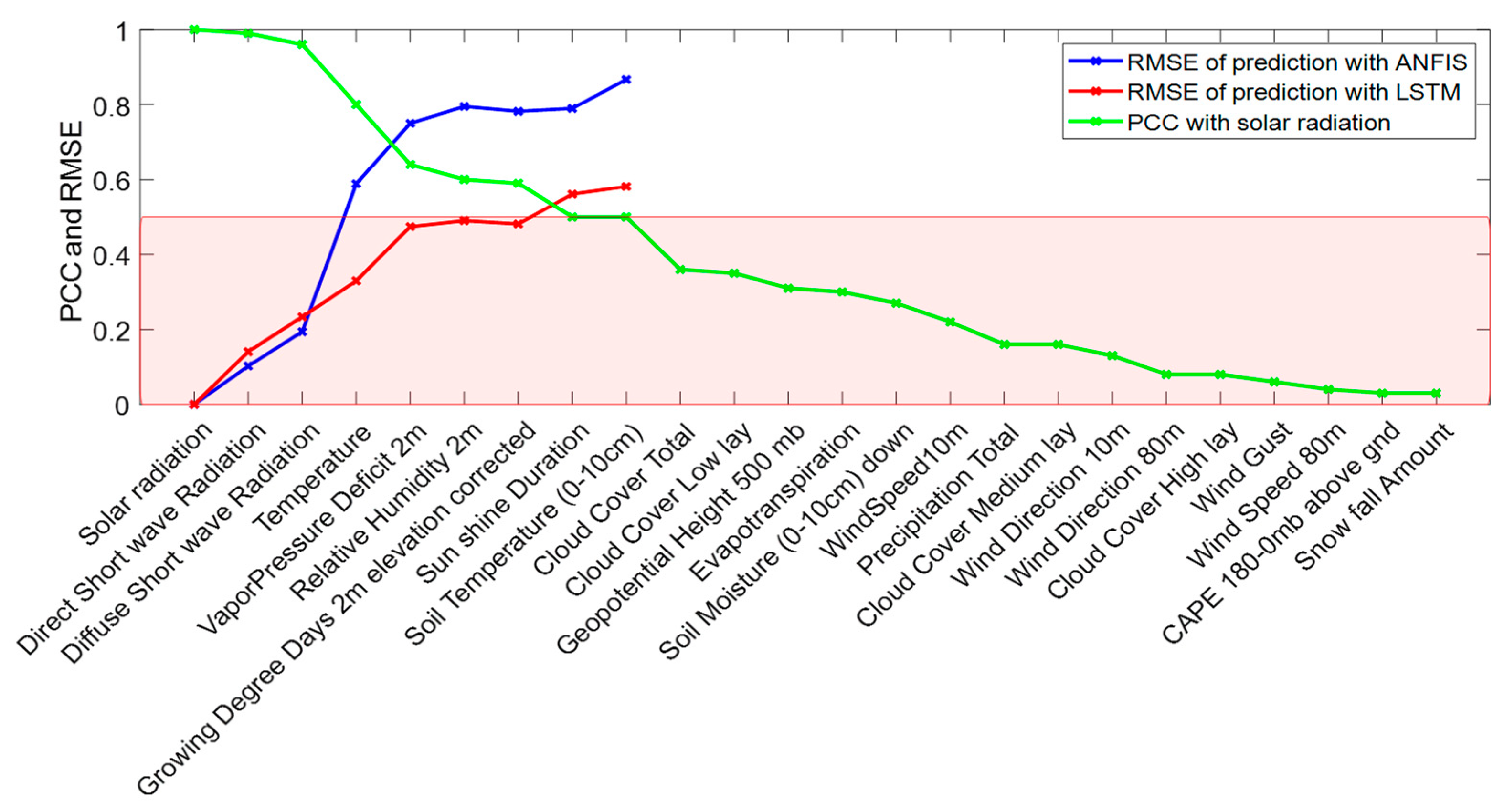
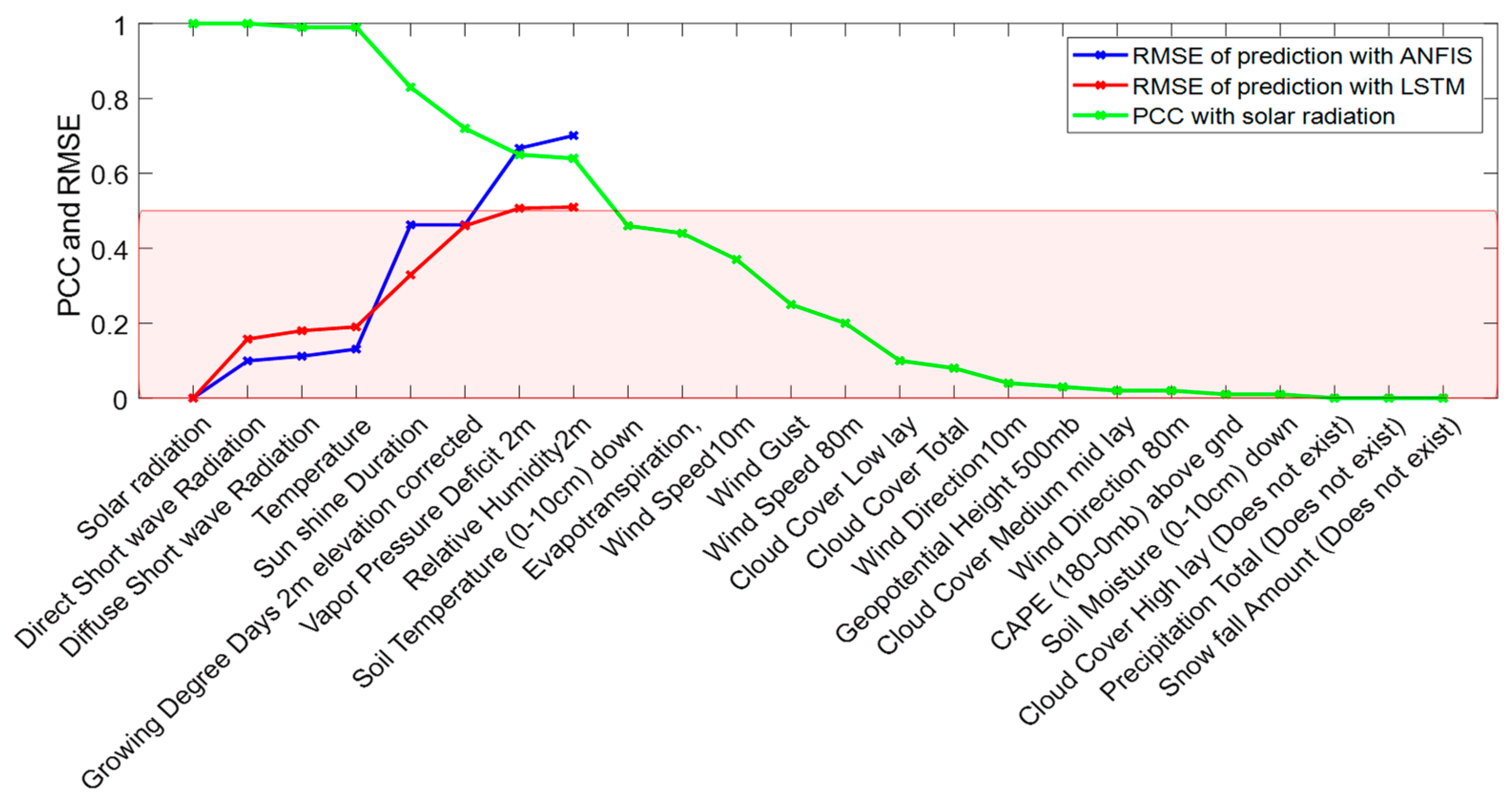
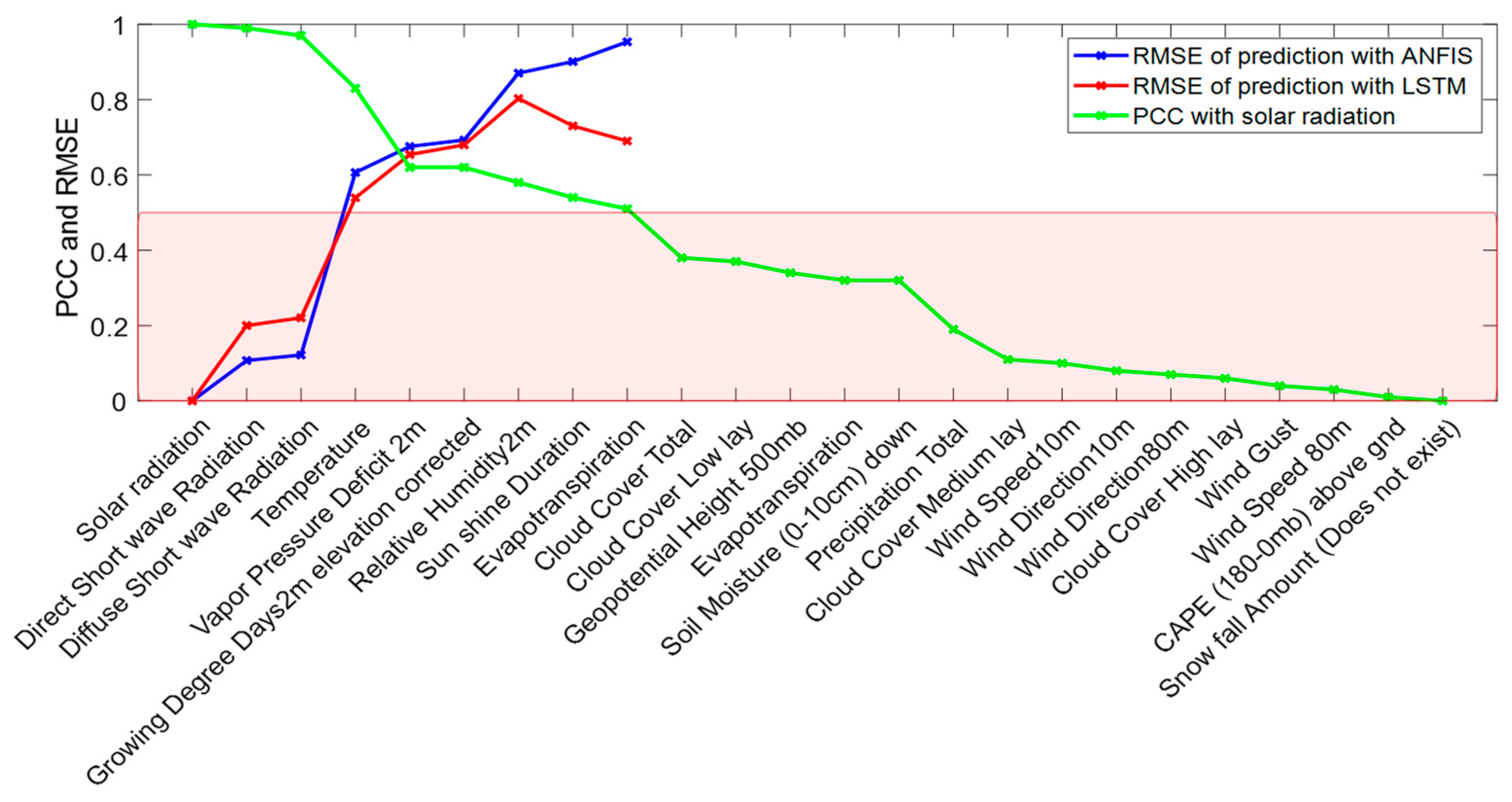
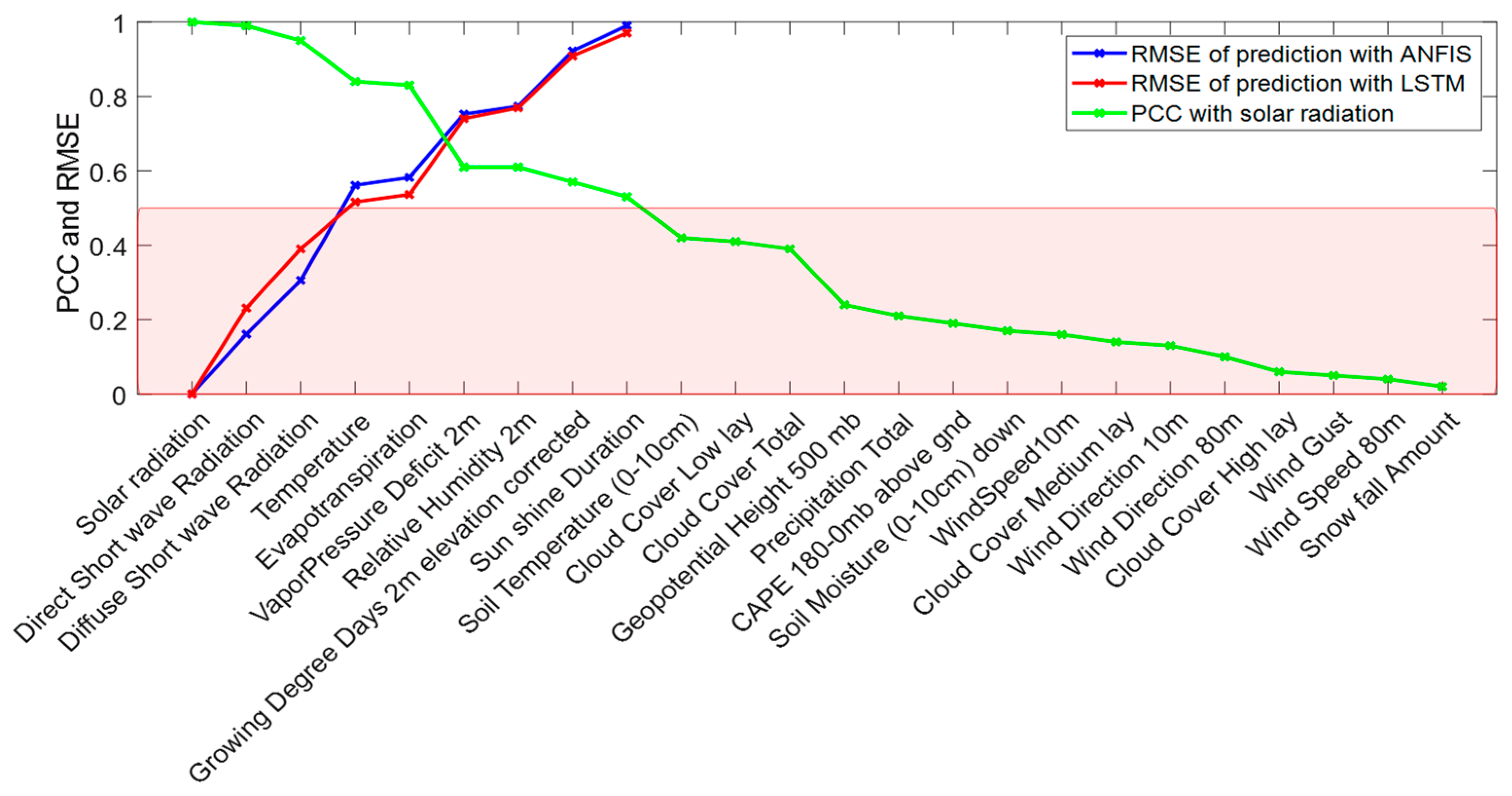
| Season | Parameters | PCC Value | Parameters | PCC Value |
|---|---|---|---|---|
| Summer | Solar radiation | 0.98 ÷ 1 | Sunshine duration | 0.5 ÷ 0.8 |
| Direct short-wave radiation | Growing degree days 2 m elevation | |||
| Diffuse short-wave radiation | Vapor pressure deficit at 2 m | |||
| Temperature | Relative humidity at 2 m | |||
| Autumn | Solar radiation | 0.98 ÷ 1 | Temperature | 0.5 ÷ 0.8 |
| Direct short-wave radiation | Vapor pressure deficit at 2 m | |||
| Diffuse short-wave radiation | Growing degree days at 2 m elevation | |||
| Relative humidity at 2 m | ||||
| Sunshine duration | ||||
| Evapotranspiration | ||||
| Winter | Solar radiation | 0.95 ÷ 1 | Temperature | 0.5 ÷ 0.8 |
| Direct short-wave radiation | Evapotranspiration | |||
| Diffuse short-wave radiation | Vapor pressure deficit at 2 m | |||
| Relative humidity at 2 m | ||||
| Growing degree days at 2 m elevation | ||||
| Sunshine duration | ||||
| Spring | Solar radiation | 0.98 ÷ 1 | Temperature | 0.5 ÷ 0.8 |
| Direct short-wave radiation | Vapor pressure deficit at 2 m | |||
| Diffuse short-wave radiation | Growing degree days at 2 m elevation | |||
| Relative humidity at 2 m |
| Reference | Test Location | Time Duration of the Study | Employed Parameters as Inputs | Machine Learning Models | Evaluation Criteria |
|---|---|---|---|---|---|
| Prado-Rujas et al. [15] | Oahu island (Hawaii) | Twenty months | Global Horizontal Irradiance (GHI), wind, longitude, latitude | RNN, LSTM, BiLSTM | RMSE less than 15% |
| Yan et al. [16] | Nevada desert, USA | One year (seasonal analysis) | Sun position, temperature, wind speed, and cloud movement. | Gated recurrent unit (GRU) NM, LSTM, | Best RMSE = 11.44 (in winter) |
| Yen et al. [17] | Southern Taiwan | Seventeen months | Temperature, humidity, rainfall, and wind speed. | SVM, RF | Best RMSE = 1.3912 |
| Lee et al. [18] | South Korea | Three years | Temperature, wind speed, humidity, and ground temperature | CNN, LSTM | Best RMSE = 0.0987 |
| Poolla et al. [19] | USA (California) | Six months | Solar irradiance, temperature, and windspeed spanning | Autoregressive ARX model | Best RMSE = 1.63 (wind) |
| Wang et al. [21] | India | One year | Historical power, solar irradiance, panel temperature. | LSTM, Conv-LSTM A-S | Best RMSE = 0.12 (Conv-LSTM-S) |
| Munir et al. [22] | Pakistan | One year | Temperature, dew point, relative humidity, and wind speed | Artificial Neural Network (ANN) | Average MAPE = 14.33% |
| Obiora et al. [23] | Johannesburg (South Africa) | Five years | Temperature, relative humidity, solar radiation, and sunshine duration | LSTM, CNN, ConvLSTM, and hybrid CNN-LSTM | Best RMSE = 7.18 (ConvLSTM) |
| de Guia et al. [24] | Morong, (Philippines) | Six month | Humidity, station temperature, ambient temperature, station altitude, sea level, absolute pressure and wind speed | ANN, CNN, bidirectional and stacked LSTM. | Best MAE = 41.738 |
| Zou et al. [25] | Scotland | Five years | Temperature, precipitation, and wind speed | Bidirectional LSTM | MAE = 0.525 (Day-ahead) 0.708 (Week-ahead) |
| Tiwari et al. [26] | Johannesburg (South Africa) | Five years | Temperature, relative humidity, solar radiation, sunshine duration | Convolutional LSTM | NRMSE = 1.62%. |
| Alvarez et al. [27] | Aguascalientes (Mexico) | Six months | Wind velocity and direction, irradiance, temperature, humidity, pressure | SVM, Linear Regression (LR) and NNMs | Mean Squared Error (MSE) 0.2222 |
| Alomari et al. [29] | Center Jordan | Thirty months | Solar radiation | ANN | RMSE = 0.0721 |
| Al-Sbou et al. [30] | South Jordan | One year | Solar radiation | ANN | MSE = 0.00237 |
| Shboul et al. [31] | North, south, center Jordan | Twenty years | Wind, air temperature, solar radiation | ANN | MAPE values < 3% |
| This research work | West-central Jordan | Five years | The 24 parameters listed in Table 1 | ANFIS, LSTM | RMSE in the range 0.04–0.8 MSE in the range 0.0016–0.64 MAE in the range 0.034–0.86 |
Publisher’s Note: MDPI stays neutral with regard to jurisdictional claims in published maps and institutional affiliations. |
© 2022 by the authors. Licensee MDPI, Basel, Switzerland. This article is an open access article distributed under the terms and conditions of the Creative Commons Attribution (CC BY) license (https://creativecommons.org/licenses/by/4.0/).
Share and Cite
Fraihat, H.; Almbaideen, A.A.; Al-Odienat, A.; Al-Naami, B.; De Fazio, R.; Visconti, P. Solar Radiation Forecasting by Pearson Correlation Using LSTM Neural Network and ANFIS Method: Application in the West-Central Jordan. Future Internet 2022, 14, 79. https://0-doi-org.brum.beds.ac.uk/10.3390/fi14030079
Fraihat H, Almbaideen AA, Al-Odienat A, Al-Naami B, De Fazio R, Visconti P. Solar Radiation Forecasting by Pearson Correlation Using LSTM Neural Network and ANFIS Method: Application in the West-Central Jordan. Future Internet. 2022; 14(3):79. https://0-doi-org.brum.beds.ac.uk/10.3390/fi14030079
Chicago/Turabian StyleFraihat, Hossam, Amneh A. Almbaideen, Abdullah Al-Odienat, Bassam Al-Naami, Roberto De Fazio, and Paolo Visconti. 2022. "Solar Radiation Forecasting by Pearson Correlation Using LSTM Neural Network and ANFIS Method: Application in the West-Central Jordan" Future Internet 14, no. 3: 79. https://0-doi-org.brum.beds.ac.uk/10.3390/fi14030079