
A Density-Based Random Forest for Imbalanced Data Classification


1
School of Computer Engineering & Science, Shanghai University, 99 Shangda Rd., Shanghai 200444, China
2
Materials Genome Institute, Shanghai University, 99 Shangda Rd., Shanghai 200444, China
3
Zhejiang Laboratory, Hangzhou 311100, China
*
Author to whom correspondence should be addressed.
Future Internet 2022, 14(3), 90; https://0-doi-org.brum.beds.ac.uk/10.3390/fi14030090
Submission received: 31 January 2022
/
Revised: 8 March 2022
/
Accepted: 9 March 2022
/
Published: 14 March 2022
(This article belongs to the Special Issue AI, Machine Learning and Data Analytics for Wireless Communications)
Abstract
:Many machine learning problem domains, such as the detection of fraud, spam, outliers, and anomalies, tend to involve inherently imbalanced class distributions of samples. However, most classification algorithms assume equivalent sample sizes for each class. Therefore, imbalanced classification datasets pose a significant challenge in prediction modeling. Herein, we propose a density-based random forest algorithm (DBRF) to improve the prediction performance, especially for minority classes. DBRF is designed to recognize boundary samples as the most difficult to classify and then use a density-based method to augment them. Subsequently, two different random forest classifiers were constructed to model the augmented boundary samples and the original dataset dependently, and the final output was determined using a bagging technique. A real-world material classification dataset and 33 open public imbalanced datasets were used to evaluate the performance of DBRF. On the 34 datasets, DBRF could achieve improvements of 2–15% over random forest in terms of the F1-measure and G-mean. The experimental results proved the ability of DBRF to solve the problem of classifying objects located on the class boundary, including objects of minority classes, by taking into account the density of objects in space.

1. Introduction
Real-world datasets generally exhibit notable imbalances between different data classes, and the effectiveness of computational classification methods is typically limited by this uneven distribution. For example, in medical cancer detection from testing data [1], relatively few samples may be expected to be detected as cancer patients, whereas most samples are normal. Similar examples have been noted in the fields of intrusion detection [2], fraud identification [3], and credit loans [4], among others. Most classification algorithms are proposed based on balanced data, and their performance is reduced when processing imbalanced data. Samples are primarily divided into majority and minority types in imbalanced datasets, according to the number of samples. Given that most classification algorithms focus on overall accuracy as their key evaluation metric, they tend to perform better when classifying samples as belonging to the majority class and heavily neglect the minority class. However, the negative effect of majority classes misclassification is less important than that of minority classes in some real application scenarios. Therefore, the development of new or improved methods to reduce the misclassification of minority classes is required.
The primary motivation of this work is to improve the prediction on minority samples in imbalanced datasets. The main idea of our proposed method is to integrate the ideas of data density with random forest classifiers to address the imbalance problem. This increases the training opportunity for minority class sets and boundary samples to reduce the misclassification of minority classes in imbalanced data. Specifically, we propose the density-based random forest (DBRF) integration method. The DBRF classifier model constructs a density domain in the sample datasets, defined as the collection of all minority and boundary samples. The poor performance of prior models is not caused by the number of categories, but rather the potential ambiguity of the decision boundary between categories. Therefore, we used ensemble learning, i.e., a random forest algorithm, to perform additional training for boundary and minority samples to improve the prediction accuracy of the model on minority samples. First, we define boundary and density domains. Then, the original dataset and these two domains are used to build the DBRF model. While improving on the sample diversity of prior models, the proposed approach is also biased toward minority samples. The contributions of this study are summarized below:
- (1)
- We used a method to identify the boundary minority samples and remove noise minority samples. The method determines whether a minority sample is a boundary minority sample or a noise sample based on the number of majority samples in its nearest neighbor samples;
- (2)
- We applied a density-based method to identify the boundary samples by boundary minority samples. The density-based method identifies the class boundary samples by taking into account the density of objects in space, as is done when solving the clustering problem with the DBSCAN algorithm;
- (3)
- A density-based random forest (DBRF) is proposed to deal with the imbalanced data problem. There are two types of classifiers in DBRF. One is built from the original dataset, and the other is constructed with boundary class samples identified by the density method, including minority class samples;
- (4)
- The performance of DBRF was evaluated based on the public binary-class-imbalanced datasets. We also compared DBRF with other common algorithms.
The remainder of this paper is organized as follows. Section 2 briefly reviews the relevant problems in this area and some related state-of-the-art approaches. Section 3 describes the improved DBRF method. Section 4 provides the experimental results and analyzes the differences between DBRF and other methods. Section 6 concludes the work and discusses some possible directions for future research.
2. Related Work
Conventional machine learning algorithms are predominantly based on balanced data; when the input data are imbalanced between classes, they cannot perform well. Generally, methods for processing imbalanced data may be divided into two categories: methods that operate at the data processing level and methods that operate at the algorithm framework level.
2.1. Data-Level Imbalanced Data Processing
At the data level, oversampling and undersampling are the main categories of methods used to process imbalanced data [5]. Oversampling balances the number of classes by duplicating the minority class samples, but this may lead to overfitting. Undersampling involves balancing the training sets by deleting some majority class samples. However, some useful information may be lost in this process, leading to underfitting.
The synthetic minority oversampling technique (SMOTE) [6] is common in practical applications. It is designed to use the nearest neighbor algorithm to select randomly N samples from the k nearest neighbors for linear interpolation, which can balance the categories in the original dataset by adding new minority class samples. Many novel methods have been proposed to further improve on this idea [7,8,9].
In classification, boundary samples are typically more likely to be misclassified. Therefore, the borderline SMOTE algorithm [10] was proposed based on the SMOTE algorithm. In contrast to other oversampling methods, the algorithm uses only relatively few class samples from the boundary samples to construct new samples.
The ADASYN algorithm [11] extends each minority class sample according to the density distribution of the training set with different weights to balance the training set. In contrast, DBRF uses the density method to find all the samples at the boundary without re-synthesizing new data points.
The compressed nearest neighbor rule (CNNR) [12] was developed to remove redundant information by undersampling the majority samples using the one-nearest neighbor algorithm and removing the majority samples far from the decision boundary. Then, a reduced dataset E is obtained from the original dataset . Because the CNNR method selects samples randomly, it causes unnecessary samples, such as noise, to remain in E.
The TomekLinks algorithm [13] is an undersampling algorithm for removing noise and boundary samples. Given two samples and from different classes, represents the distance between the two samples. If no sample x meets the conditions that or , the sample pair constitutes a TomekLink. Either one of the two samples in TomekLink is noise or both are on the boundary of the two types. Using this property, the method can delete the noise and redundant samples by constituting the TomekLinks.
The one-sided selection algorithm (OSS) [14] attempts intelligent undersampling of most classes by removing redundant data or artificial noise.
The edited nearest neighbor (ENN) algorithm [15] reduces majority samples through a 3NN method. First, the ENN finds three samples that have the nearest distances to a certain sample x. Then, if two or more of them have a different class than the sample x, the sample x is deleted. Because most samples are often surrounded by majority classes, relatively few majority samples are deleted by the ENN algorithm. Therefore, the neighborhood cleaning rule [16] was modified from the ENN. If the sample is a majority sample, it will do the same as the ENN. Majority samples are removed if the sample is a minority sample and more than two of three samples chosen by the 3NN are majority samples.
2.2. Algorithm-Level Methods for Imbalanced Data
Three approaches for imbalanced datasets at the algorithmic level are predominantly used: cost-sensitive learning [17], ensemble learning [18], and single-class classification [19]. Cost-sensitive learning methods apply various misclassification costs to classification decision-making. The goal is to minimize the overall misclassification cost rather than reduce the error rate. When the amount of data between categories is severely imbalanced, the classifier tends to predict all testing data as belonging to a majority category. To solve this problem, a classification method based on distinction is no longer applicable; therefore, a method based on learning recognition and single-class learning is proposed herein. The single-class learning method is designed to learn only the samples of the target class of interest, that is to train only the samples of majority classes and to fully learn their features. The goal is to identify the majority class sample from the test sample instead of distinguishing whether a sample belongs to the minority or majority class. A new sample is distinguished by comparing the similarities between the sample and the target class.
In ensemble learning, multiple basic learners are combined to obtain better generalization performance than a single classifier [18]. Three approaches have been explored for ensemble-learning-based imbalanced data processing: data resampling combined with ensemble learning, cost-sensitive learning combined with ensemble learning, and increasing the diversity of classifiers in ensemble learning. SMOTEBoost [20] is a combination of SMOTE and AdaBoost [21]. First, the SMOTE algorithm is used to generate new minority samples in each iteration. Then, the minority samples receive more attention in the next iteration. Because each base classifier is constructed using different training sets, this method improves the decision domain after the vote integration. Chen et al. [22] developed a method that combines oversampling and undersampling and is effective for highly imbalanced data. First, it balances the sample set with undersampling and then optimizes the basic properties of the dataset, such as the data distribution and diversity, by oversampling.
The AdaCost algorithm [23] improves the recall rate and accuracy of the boosting algorithm [24] by introducing the misclassification cost of each training sample during the weight update of the boosting algorithm. In AdaCost, the weight update rule is as follows: (1) if the weak classifier misclassifies the samples with higher misclassification cost, its weight is increased; (2) if it classifies correctly, its weight is decreased.
Chen et al. [25] proposed the random forest variants balanced random forest (BRF) and weighted random forest (WRF). BRF performs the random replication of the minority class when constructing the training subset. WRF integrates the idea of cost-sensitive learning with random forest classifiers, that is increasing the weight of minority classes. Meanwhile, during voting, the weight multiplied by the number of votes is used as the final result. The weight is updated using the out-of-bag error data. These methods improve the data prediction of the algorithm.
The imbalance problem involves other factors in addition to class bias, such as class overlap, decision boundaries, and sample distribution. Choudhary and Shukla [26] proposed an algorithm that decomposes the complex imbalance problem into simpler sub-problems by a fuzzy clustering method and then assigns weights to each sub-classifier for voting classification.
Biased random forest (BRAF) [27] reduces the prediction error rate of minority classes by increasing the diversity of ensemble learning. First, undersampling is used to construct the critical areas on the original dataset. Then, the critical areas are used to train the subtree. Finally, the trained subtree is merged with the standard random forest. A new method based on an information granule (IGRF) [28] applied the idea of BRAF to crime detection. The IGRF process combines information granularity and the series of crime pairs in k neighbors to form the critical areas. Then, the same procedure as BRAF is used to construct the model.
With the widespread use of deep learning, some scholars have studied the class-balanced loss function, distinct block processing of images, data augmentation techniques, etc. Olusola et al. [29] proposed a novel data augmentation technique based on covariate synthesis minority oversampling (SMOTE) to address data scarcity and category imbalance. Jeyaprakash et al. [30] proposed an efficient malware detection system based on deep learning to address imbalances in malware datasets. Oyewola et al. [31] proposed a novel deep residual convolutional neural network (DRNN) for cassava mosaic disease detection in cassava leaf images. Inzamam et al. [32] proposed a new data augmentation technique that uses the secondary dataset RVL-CDIP to normalize imbalanced datasets.
To sum up, on the data level, oversampling methods (SMOTE, ADASYN, etc.) balance the dataset for classification by adding minority samples. If there are too many noise samples in the minority samples, the distribution of the original dataset will change after the sample expansion. Undersampling methods (ENN, etc.) balance the dataset by reducing the number of majority samples. For highly imbalanced datasets, deleting too many valid samples makes it impossible to fully train the dataset. On the algorithm level, BRAF finds the k-nearest majority neighbors for each minority sample. Then, it merges the k-nearest majority neighbors with the minority samples directly to construct critical areas. The method used in BRAF cannot identify boundary samples accurately and introduces noise and redundant samples. It also impacts the subsequent classifications. To solve this problem, we propose a DBRF algorithm. DBRF obtains a random forest using the density distribution method to build the density domain based on BRAF. DBRF constructs the density domain based on the boundary minority samples. The aim of the study was to locate samples lacking a clear decision boundary and enhance the ability to identify them.
3. Methods
Inspired by the borderline SMOTE [10], DBSCAN [33], and BRAF [27] algorithms, we herein propose DBRF to solve the problem of insufficient prediction accuracy for minority classes in imbalanced datasets. The DBRF algorithm has two main purposes. (1) Additional training is performed on boundary samples. In the imbalanced dataset, the main factor resulting in the poor performance of prior models is not the balance of the number of categories between classes, but the ambiguity of the decision boundaries between the categories. Therefore, additional training can be performed on the boundary samples to reduce the prediction error rate of the minority class by increasing the diversity of the model. (2) The additional training samples are constructed to meet the minority sample distribution as much as possible through the density method, aiming to accurately locate samples with unclear decision boundaries, referred to as boundary samples.
Therefore, our objective was to locate boundary samples as accurately as possible. We define two domains: boundary and density domains. These domains are constructed to locate the boundary samples more accurately for additional training. The boundary domain functions to determine the boundary minority samples. We aimed to find the boundary minorities to determine the final dataset for additional training because it is mainly used to improve the prediction of minority classes. The density domain functions to locate the boundary samples, that is the final dataset, for additional training. The density domain serves to determine the majority class samples by density, that is the majority class samples according to the distribution of the boundary minority class samples. Figure 1 shows an imbalanced dataset. In Figure 1, the green, gray, and red points represent the samples used for additional training.
3.1. Definition
3.1.1. Boundary Domain
This is a set of minority samples and requires that the number of majority samples in the m-nearest neighbors of the minority samples be greater than the number of minority samples.
In Equation (1), represents the i-th sample in minority class , s represents the total number of minority samples, m represents the number of neighboring samples to be selected, D represents the original dataset, represents the Euclidean distance from sample to all samples in the original dataset D, and represents the number of samples of the majority class in the first m samples near the sample .
3.1.2. Direct Density-Reachability and Density-Reachability
Before introducing the density domain, we introduce two core concepts defined in DBSCAN: direct density-reachability and density-reachability. These two concepts are used when defining the density domain:
- -
- Direct density-reachability: If , and , then sample is directly-reachable by the density of , where , . Here, represents the set of majority class samples, represents the distance between samples and , represents the maximum distance that can reach, represents a set of majority samples whose distance from sample is less than or equal to , and represents the total number of sets. represents the minimum number of sets whose distances between the samples in the set and sample are less than or equal to ;
- -
- Density-reachability: For samples and , if there are sample sequences where , , and is directly density-reachable by , then it is said that is density-reachable by .
3.1.3. Density Domain
This is a set consisting of the majority class samples around the boundary domain and the minority class samples in the original dataset. More specifically,
In Equation (2), represents the minority class set, and Z represents all sample sets whose density can be reached by the boundary domain samples. Therefore, Z can be defined by Equation (3), where is the set of majority class samples.
Figure 2 shows an example of direct density-reachability and density-reachability.
The most notable aspect of the proposed approach is the integration of oversampling and undersampling. However, the distinction between the process of DBRF and undersampling and oversampling is that DBRF uses the characteristics of ensemble learning to improve the results at the algorithmic model level, rather than at the data processing level.
3.2. DBRF Algorithm
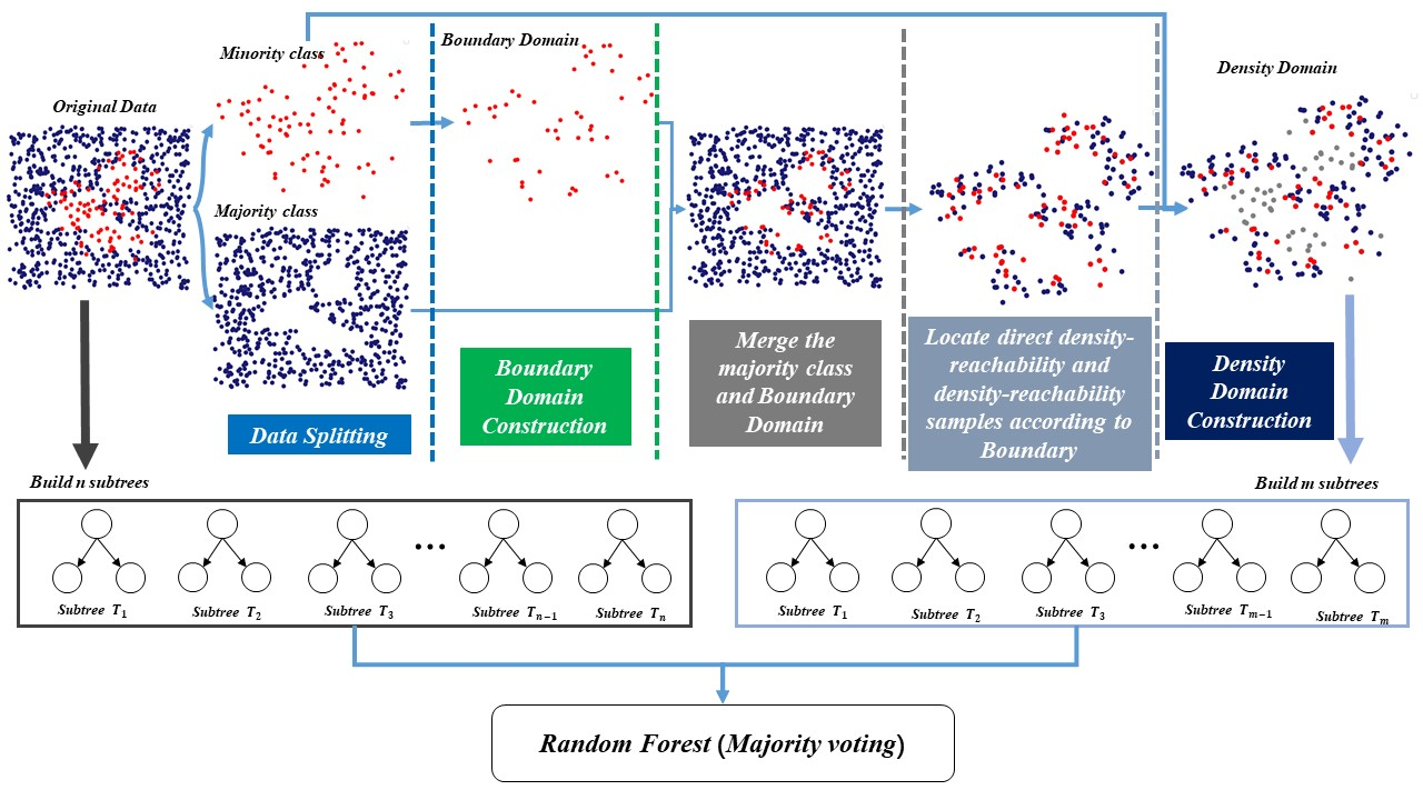
An overview of the entire DBRF procedure is shown in Figure 3, divided into four steps: data splitting, boundary domain construction, density domain construction, and model merging.The details of the algorithm are presented in Algorithm 1.
For data splitting, the original dataset was divided into majority and minority sets. The details of the algorithm are presented in Algorithm 2. The boundary domain construction first counts , which is the number of majority classes in m neighbors of a single minority sample in the original dataset. Then, if , the sample is added to the boundary domain. This is shown by the gray triangles in Figure 1. The details of the algorithm are presented in Algorithm 3.
Density domain construction determines the majority class samples based on the distribution of the boundary minority class samples. DBRF uses the clustering method to identify the boundary samples from boundary minority samples, as is done when solving the clustering problem with the DBSCAN algorithm. Then, it merges them with the minority class to build the density domain. The green, gray, and red sample points in Figure 1 represent the density domain. The details of the algorithm are presented in Algorithm 4.
| Algorithm 1Density-based random forest (DBRF). |
|
| Algorithm 2Data splitting. |
|
| Algorithm 3Boundary domain construction. |
|
| Algorithm 4Density domain construction. |
|
4. Experimental Setup and Results’ Analysis
4.1. Experimental Dataset
In this study, imbalanced datasets from different areas were used to evaluate the DBRF algorithm with three categories of data. Dataset (A) contained metal glass, vehicle evaluation, and Haberman’s survival. The metal glass data were obtained from [34]. The vehicle evaluation and Haberman’s survival data were obtained from the UCI open database [35]. Dataset (B) contained a combination of 19 real datasets. Dataset (C) contained 12 synthetic datasets. The 19 real datasets and 12 synthetic datasets were obtained from the Keel database [36].
For Dataset (A), vehicle assessment and Haberman’s survival were classified into two categories. The metal glass data were classified into three categories—crystalline alloy (CRA), ribbon metallic glass (RMG), and bulk metallic glass (BMG)—in a ratio of 6:3:1. BMG has excellent material properties, whereas the others do not, such as wear resistance and high yield strength [34,37,38,39]. Therefore, we focused more on BMGs.
For Dataset (B), each of the 19 real datasets was a two-category dataset, and the imbalance ratio was distributed from 1.82 to 25.58. For each of the datasets, the number of samples ranged from 173 to 5472.
For Dataset (C), the 12 synthetic datasets were divided into three categories: clover, paw, and subclus. To increase the classification difficulty, the degree of confusion in the minority and majority classes in each category was increased by 30%, 50%, and 70%, respectively. Each dataset was a two-category dataset with 800 samples, and the imbalance ratio was 1:7. The detailed information of the datasets is shown in Table 1, including the imbalance ratio, sample size, number of minority classes, dataset names, number of features, and number of majority classes.
The experimental environment was Windows 10, 64 bit edition, with Python 3.7.7, sklearn 0.23.2, pandas 1.0.5, and imblearn 0.7.0.
4.2. Algorithm Evaluation Indicators
The performance metrics compared in this study were principally the overall accuracy rate (accuracy), recall, precision, F1-measure (F1), and G-mean (GM). Ten-fold cross evaluation was performed for each dataset. F1 is based on the harmonic average of recall and precision. GM attempts to maximize the accuracy of each class while maintaining a balance of accuracy. For imbalanced data, it is typically inadvisable to evaluate the performance of classifier models in terms of accuracy. In Equation (8), m represents the total number of categories. F1 and GM are unbiased evaluation indicators for imbalanced classification. In imbalanced classification tasks, F1 and GM can better evaluate model performance compared to accuracy, recall, and precision; therefore, we mainly compared F1 and GM. Table 2 shows the confusion matrix used in the two-class classification in this experiment [40]. True positive (TP) indicates the number of samples in which the original class and predicted class are both minority classes. False positive (FP) indicates the number of samples in which the original class is a majority class, whereas the predicted class is a minority class. True negative (TN) indicates the number of samples in which the original class and the predicted class are both majority classes. False negative (FN) indicates the number of samples in which original class is the minority class, whereas the predicted class is the majority.
4.3. Experimental Results and Analysis
4.3.1. Parameter Setting on and p
We compared the random forest and DBRF algorithms on the metal glass, vehicle evaluation, and Haberman’s survival data. To make the experimental results more comparable, the relevant parameters involved in the models were consistent. The RF model only involves the number of trees . The DBRF model involves neighborhood distance , minimum number of samples in the domain , allocation ratio of trees p, and number of trees .
In DBRF, owing to the different datasets, the neighborhood distance correspondingly differed. First, was set as the average of the nearest neighbor distances of 20 majority class samples of a certain minority sample. Then, we adjusted the parameter based on . Figure 4 shows the trend of the density domain as changes. Figure 4 indicates that as increases, the majority class samples gradually increased until all the majority class samples were selected. With the increase of the selected majority class samples, the role played by the density domain gradually became smaller, which deviated from our aim in proposing DBRF to improve the prediction of minority classes through additional training boundary samples. Therefore, choosing a suitable significantly impacts the performance of predictions involving minority classes.
Figure 5 presents the experimental results obtained on the metal glass, vehicle evaluation, and Haberman’s survival data with different values of . Each point in the figure represents the average value of the ten-fold cross-validation experiments. The experimental results were consistent with our expectations. For example, as increased, the accuracy gradually increased, whereas F1 and GM gradually decreased. This means that the role of the density domain gradually weakened. When all the samples were included, it was equivalent to training a random forest classifier with the original dataset, nullifying the performance improvement of the proposed approach.
For the metal glass dataset, GM decreased as increased, whereas F1 and Accuracy increased. The main reason for the growth of F1 is that as the number of majority classes increased, the model’s prediction accuracy gradually increased for the majority class and gradually decreased for the minority class samples. The increase in the majority class compensated for the decreases in the minority class, resulting in an increase in F1 with increasing .
For the Haberman’s survival dataset, both GM and F1 decreased with increasing , and accuracy increased with increasing . The experimental results were consistent with our expectations.
For the vehicle evaluation dataset, accuracy, F1, and GM first decreased and then gradually stabilized as increased. This shows that for the vehicle evaluation dataset could only be adjusted to one. When , the density domain contained all the majority samples. Therefore, there was a sharp drop when and .
Figure 6 presents the results obtained on the metal glass, vehicle evaluation, and Haberman’s survival datasets with different values of p. It can be observed that the overall accuracy decreased as p increased in Figure 6. Although the recall of the minority class increased with increasing p, the majority class was also miscategorized. Through F1 and GM, the results showed that after , the performance of the model began to decline, mainly because the prediction accuracy of the majority class began to decline. Therefore, for the metal glass dataset, p was set at 0.4.
In Figure 6, for the vehicle evaluation dataset, it can be observed that DBRF outperformed the base model RF for F1 and GM. The reason that DBRF was higher in F1, GM, and accuracy than those of RF was mainly that the TP of the other two models was very low, while DBRF compensated for the drop in FP due to the increase in TP. Therefore, the F1 and GM of DBRF were higher than those of RF. Therefore, the best p value for the vehicle evaluation dataset was 0.5.
In Figure 6, for the Haberman’s survival dataset, it can be seen that the F1 and GM of DBRF were higher than those of RF. To avoid losing too much overall accuracy, we set . When , the F1 and GM of the DBRF were improved, and the overall accuracy loss was less.
Figure 7 shows a box plot of the 10-fold cross-validation on the three datasets with the best p and . Figure 7 indicates that the maximum value of DBRF was larger than that of the base algorithm RF, and the minimum value was larger than that of RF. In addition, the distribution of the 10 experimental results revealed that DBRF was relatively stable.
4.3.2. Performance on Public Imbalanced Datasets
In this experiment, we first compared random forest with DBRF and then the random forest combined with oversampling methods through the remaining 19 datasets and 12 synthetic datasets. The oversampling methods included SMOTE, borderline SMOTE, and ADASYN. The comparison experiment was conducted to evaluate whether DBRF is effective at handling imbalanced datasets.
In Table 3, (A) shows the F1 and GM results for metal glass, vehicle evaluation, and Haberman’s survival. Figure 8 shows the averaging confusion matrices of metal glass. In Figure 8, DBRF exhibited better prediction accuracy for BMG than RF. Compared to other algorithms, DBRF was less competitive, but had better performance on F1 and GM. Figure 9 shows the averaging AUC curve and ROC of metal glass. DBRF had good performance on the AUC and ROC curve compared with the other algorithms.
In Table 3, (B) shows the F1 and GM results for the 19 public imbalanced datasets. DBRF improved F1 by 2–5% compared with the other models. DBRF was more competitive than the other models in most imbalanced datasets. ADASYN + RF, RF, b-SMOTE + RF, and ADASYN + RF were more competitive than DBRF on glasses1, dermatology, page-blocks0, Vehicle0, Vehicle1, and Vehicle2. DBRF improved the GM by 2–6% compared with the other models. Specifically, DBRF was more competitive than RF on the 19 public imbalanced datasets. SMOTE + RF, b-SMOTE + RF, and ADASYN + RF outperformed DBRF on glassed1, car-good, car-vgood, page-blocks0, Vehicle0, Vehicle1, and Vehicle2.
In Table 3, (C) shows the average value of 12 synthetic datasets after 10-fold cross-validation. Among all 12 datasets, the difficulty increased with the number of interference samples. For example, in Paw0, the boundary between the minority class and the majority class was clear, and F1 and GM were generally high. However, in the Paw70 dataset, the boundary was unclear. As the number of interference samples increased, F1 and GM began to decline, indicating that the decision boundary between the minority class and the majority class began to become difficult to distinguish. For F1 and GM, DBRF was best on most datasets. In particular, DBRF was more competitive than RF on GM. This indicates that our proposed model can achieve an improvement in the minority class prediction accuracy over prior methods while remaining relatively stable even when the decision boundary is very difficult to distinguish.
Table 4 shows the average time during training for RF, DBRF, SMOTE + RF, b-SMOTE + RF, and ADASYN + RF. As the number of features and samples in the dataset increased, DBRF took more time to train the model than other algorithms. In particular, DBRF took twice the time of RF on the metal glass and page-blocks0 datasets.
We used the Wilcoxon signed rank test, which is a non-parametric test, to statistically analyze the results of the experiments on 34 datasets. The function of the Wilcoxon signed-rank test is to determine whether the corresponding overall distribution of the data is the same without assuming that the data obey a normal distribution. In this test, the confidence interval was set at 0.05. When the test yields a p-value significantly less than 0.05, the two methods are significantly different. From Table 5, it can be seen that the p-values for DBRF versus RF, SMOTE + RF, b-SMOTE + RF, and ADASYN + RF were all less than 0.05. This suggests that the differences between them were significant. It also indicates that DBRF was more competitive than the other models in handling imbalanced data.
5. Discussion
Despite its performance, DBRF has the following limitations:
- (1)
- Parameter setting problem. DBRF has two parameters, and p. Figure 4, Figure 5 and Figure 6 show that different parameters need to be set for different datasets. If is too large, the density domain will have all samples in the dataset. This results in the failure of DBRF to classify the minority class. Choosing which parameters to use to train the model requires some tuning experience;
- (2)
- Questions about datasets. For this question, there are two main problems: (a) Time-consuming problem. DBRF can effectively train large datasets, but it takes much time in the training process. Metal glass is a dataset with 98 features and 5936 samples. It is the largest of the 34 datasets. According to the experimental results in Table 2, DBRF took more time to train on it than other algorithms. Therefore, for large datasets with high-dimensional features, the training time of DBRF will obviously become long; (b) The number of minority class samples problem. DBRF will be ineffective if the dataset has few minority class samples. Owing to the excessively scattered distribution of minority class samples, they will be deleted as noise samples when DBRF constructs the boundary domain. This will lead to an inability to build the density domain. Our proposed method will not work;
- (3)
- The problem of unclear decision boundaries between minority classes. DBRF cannot solve this problem. DBRF can just deal with the problem of the unclear decision boundary between majority samples and minority samples. This is because DBRF takes one class from the minority class group separately as the only minority class for density domain construction.
6. Conclusions and Future Work
We proposed a density-based random forest algorithm (DBRF) to improve the prediction performance, especially for minority classes. We aimed to improve the original random forest algorithm in a way that enhances its performance on imbalanced sets. To achieve this aim, we proposed to borrow some ideas from the DBSCAN algorithm. In particular, we took into account the density of objects in space to improve the prediction performance, especially for minority classes. At the same time, we considered already known approaches for the development of classifiers for imbalanced datasets, including the SMOTE algorithm. DBRF was designed to recognize boundary objects, and it uses a density-based method to recognize them. Two different random forest classifiers were constructed to model the augmented boundary objects and the original dataset dependently, and the final output was determined using a bagging technique. Table 3 shows the average of 34 public imbalanced datasets. Our proposed method (DBRF) was the best among the five algorithms. On F1, DBRF improved classification by 1.7–2.5% on average. On GM, DBRF there was an improvement of approximately 1–2.5% on average. The experimental results proved the ability of the proposed algorithm (DBRF) to solve the problem of classifying objects located on the class boundary, including objects of minority classes, by taking into account the density of objects in space (as is done when solving the clustering problem with the DBSCAN algorithm).
Several directions deserve further study in the future. First, in imbalanced data processing, the imbalance is caused by a variety of factors. To address this problem, the integration of domain knowledge into the classification models is very important. Second, we used a random forest classifier as the basic model, which suggests that our density-based method may also be effective for other models, such as XGBoost, LightGBM, and neural networks. Finally, data labeling is time-consuming; thus, methods to utilize the unlabeled data in imbalanced data classification also constitute an interesting potential avenue for future research.
Author Contributions
Conceptualization, Q.Q.; Data curation, J.D.; Software, J.D.; Supervision, Q.Q.; Writing—original draft, J.D.; Writing—review & editing, Q.Q. All authors have read and agreed to the published version of the manuscript.
Funding
This work was sponsored by the National Key Research and Development Program of China (Grant No. 2018YFB0704400), the Key Program of Science and Technology of Yunnan Province (No. 202102AB080019-3, 202002AB080001-2), the Key Research Project of Zhejiang Laboratory (No. 2021PE0AC02), and the Key Project of Shanghai Zhangjiang National Independent Innovation Demonstration Zone (No. ZJ2021-ZD-006).
Data Availability Statement
All the datasets and source code that support the experimental findings can be accessed at: https://github.com/qq-shu/DBRF (accessed on 8 May 2021).
Acknowledgments
The authors gratefully appreciate the anonymous Reviewers for their valuable comments.
Conflicts of Interest
The authors declare no conflict of interest.
References
- Zhang, J.; Cao, P.; Gross, D.P.; Zaiane, O.R. On the application of multi-class classification in physical therapy recommendation. Health Sci. Syst. 2013, 1, 15. [Google Scholar] [CrossRef] [Green Version]
- Zhang, Y.; Zhang, H.; Zhang, X.; Qi, D. Deep learning intrusion detection model based on optimized imbalanced network data. In Proceedings of the 2018 IEEE 18th International Conference on Communication Technology (ICCT), Chongqing, China, 8–11 October 2018. [Google Scholar]
- Bian, Y.; Cheng, M.; Yang, C.; Yuan, Y.; Li, Q.; Zhao, J.L.; Liang, L. Financial fraud detection: A new ensemble learning approach for imbalanced data. In Proceedings of the 20th Pacific Asia Conference on Information Systems (PACIS 2016), Chiayi, Taiwan, 27 June–1 July 2016; p. 315. [Google Scholar]
- Plant, C.; Böhm, C.; Tilg, B.; Baumgartner, C. Enhancing instance-based classification with local density: A new algorithm for classifying unbalanced biomedical data. Bioinformatics 2006, 22, 981–988. [Google Scholar] [CrossRef] [Green Version]
- Yap, B.W.; Rani, K.A.; Rahman, H.A.A.; Fong, S.; Khairudin, Z.; Abdullah, N.N. An application of oversampling, undersampling, bagging and boosting in handling imbalanced datasets. In Proceedings of the First International Conference on Advanced Data and Information Engineering (DaEng-2013), Kuala Lumpur, Malaysia, 16–18 December 2013; Springer: Berlin/Heidelberg, Germany, 2014; pp. 13–22. [Google Scholar]
- Chawla, N.V.; Bowyer, K.W.; Hall, L.O.; Kegelmeyer, W.P. Smote: Synthetic minority over-sampling technique. J. Artif. Res. 2002, 16, 321–357. [Google Scholar] [CrossRef]
- Bunkhumpornpat, C.; Sinapiromsaran, K.; Lursinsap, C. Dbsmote: Density-based synthetic minority over-sampling technique. Appl. Intell. 2012, 36, 664–684. [Google Scholar] [CrossRef]
- Ma, L.; Fan, S. Cure-smote algorithm and hybrid algorithm for feature selection and parameter optimization based on random forests. BMC Bioinform. 2017, 18, 169. [Google Scholar] [CrossRef] [PubMed] [Green Version]
- Gao, M.; Aiqiang, X.U.; Qing, X.U. Fault detection method of electronic equipment based on sl-smote and cs-rvm. Comput. Eng. Appl. 2019, 55, 185–192. [Google Scholar]
- Han, H.; Wang, W.-Y.; Mao, B.-H. Borderline-smote: A new over-sampling method in imbalanced datasets learning. In Proceedings of the International Conference on Intelligent Computing, Hefei, China, 23–26 August 2005; Springer: Berlin/Heidelberg, Germany, 2005; pp. 878–887. [Google Scholar]
- He, H.; Bai, Y.; Garcia, E.A.; Li, S. Adasyn: Adaptive synthetic sampling approach for imbalanced learning. In Proceedings of the 2008 IEEE International Joint Conference on Neural Networks (IEEE World Congress on Computational Intelligence), Hong Kong, 1–8 June 2008; pp. 322–1328. [Google Scholar]
- Batista, G.E.; Prati, R.C.; Monard, M.C. A study of the behavior of several methods for balancing machine learning training data. ACM Sigkdd Explor. Newsl. 2004, 6, 20–29. [Google Scholar] [CrossRef]
- Tomek, I. Two modifications of cnn. IEEE Trans. Syst. Man Cybern. 1976, SMC-6, 769–772. [Google Scholar]
- Kubat, M.; Matwin, S. Addressing the curse of imbalanced training sets: One-sided selection. Icml 1997, 97, 179–186. [Google Scholar]
- Wilson, D.L. Asymptotic properties of nearest neighbor rules using edited data. IEEE Trans. Syst. Man Cybern. 1972, SMC-2, 408–421. [Google Scholar] [CrossRef] [Green Version]
- Laurikkala, J. Improving identification of difficult small classes by balancing class distribution. In Proceedings of the Conference on Artificial Intelligence in Medicine in Europe, Cascais, Portugal, 1–4 July 2001; Springer: Berlin/Heidelberg, Germany, 2001; pp. 63–66. [Google Scholar]
- Zhou, Z.-H.; Liu, X.-Y. Training cost-sensitive neural networks with methods addressing the class imbalance problem. IEEE Trans. Knowl. Data Eng. 2005, 18, 63–77. [Google Scholar] [CrossRef]
- Zhou, Z.-H. Ensemble Learning: Foundations and Algorithms; Electronic Industry Press: Beijing, China, 2020. [Google Scholar]
- Raskutti, B.; Kowalczyk, A. Extreme re-balancing for svms: A case study. ACM Sigkdd Explor. Newsl. 2004, 6, 60–69. [Google Scholar] [CrossRef]
- Chawla, N.V.; Lazarevic, A.; Hall, L.O.; Bowyer, K.W. Smoteboost: Improving prediction of the minority class in boosting. In Proceedings of the European Conference on Principles of Data Mining and Knowledge Discovery, Antwerp, Belgium, 15–19 September 2003; Springer: Berlin/Heidelberg, Germany, 2003; pp. 107–119. [Google Scholar]
- Freund, Y.; Schapire, R.E. A decision-theoretic generalization of on-line learning and an application to boosting. J. Ournal Comput. And Syst. Sci. 1997, 55, 119–139. [Google Scholar] [CrossRef] [Green Version]
- Chen, Z.; Duan, J.; Kang, L.; Qiu, G.-Q. A hybrid data-level ensemble to enable learning from highly imbalanced dataset. Inf. Sci. 2021, 554, 157–176. [Google Scholar] [CrossRef]
- Fan, W.; Stolfo, S.J.; Zhang, J.; Chan, P.K. Adacost: Misclassification cost-sensitive boosting. Icml 1999, 99, 97–105. [Google Scholar]
- Schapire, R.E.; Freund, Y. Boosting: Foundations and algorithms. Kybernetes 2013, 42, 164–166. [Google Scholar] [CrossRef]
- Chen, C.; Breiman, L. Using Random Forest to Learn Imbalanced Data; University of California: Berkeley, CA, USA, 2004. [Google Scholar]
- Choudhary, R.; Shukla, S. A clustering based ensemble of weighted kernelized extreme learning machine for class imbalance learning. Expert Syst. Appl. 2021, 164, 114041. [Google Scholar] [CrossRef]
- Bader-El-Den, M.; Teitei, E.; Perry, T. Biased random forest for dealing with the class imbalance problem. IEEE Trans. Neural Netw. Learn. Syst. 2018, 30, 2163–2172. [Google Scholar] [CrossRef] [Green Version]
- Li, Y.-S.; Chi, H.; Shao, X.-Y.; Qi, M.-L.; Xu, B.-G. A novel random forest approach for imbalance problem in crime linkage. Knowl.-Based Syst. 2020, 195, 105738. [Google Scholar] [CrossRef]
- Oyewola, D.O.; Dada, E.G.; Misra, S.; Damaeviius, R. Detecting cassava mosaic disease using a deep residual convolutional neural network with distinct block processing. PeerJ Comput. Sci. 2021, 7, E352. [Google Scholar] [CrossRef]
- Hemalatha, J.; Roseline, S.A.; Geetha, S.; Kadry, S.; Damaeviius, R. An Efficient DenseNet-Based Deep Learning Model for Malware Detection. Entropy 2021, 23, 344. [Google Scholar] [CrossRef] [PubMed]
- Alli, O.O.A.; Damaeviius, R.; Misra, S.; Rytis, M.; Alli, A.A. Malignant skin melanoma detection using image augmentation by oversampling in nonlinear lower-dimensional embedding manifold. Turk. J. Electr. Eng. Comput. Sci. 2021, 2021, 2600–2614. [Google Scholar] [CrossRef]
- Nasir, I.M.; Khan, M.A.; Yasmin, M.; Shah, J.H.; Damasevicius, R. Pearson Correlation-Based Feature Selection for Document Classification Using Balanced Training. Sensors 2020, 20, 6793. [Google Scholar] [CrossRef] [PubMed]
- Ester, M.; Kriegel, H.-P.; Sander, J.; Xu, X. A density-based algorithm for discovering clusters in large spatial databases with noise. Kdd 1996, 96, 226–231. [Google Scholar]
- Zhang, L.; Huang, H. Micro machining of bulk metallic glasses: A review. Int. J. Adv. Manuf. Technol. 2018, 100, 637–661. [Google Scholar] [CrossRef]
- Dua, D.; Graff, C. UCI Machine Learning Repository. 2017. Available online: http://archive.ics.uci.edu/ml (accessed on 8 May 2012).
- Alcalá-Fdez, J.; Fernandez, A.; Luengo, J.; Derrac, J.; García, S.; Sánchez, L.; Herrera, F. Keel data-mining software tool: Data set repository, integration of algorithms and experimental analysis framework. Crit. Rev. Solid State Mater. Sci. 2011, 17, 255–287. [Google Scholar]
- Mehdi, J.Z.; Gideon, P.K.; Paulo, B.; Mohsen, S.; John, L.; Cui, F. A critical review on metallic glasses as structural materials for cardiovascular stent applications. J. Funct. Biomater. 2018, 9, 19. [Google Scholar]
- Khan, M.M.; Nemati, A.; Rahman, Z.U.; Shah, U.H.; Asgar, H.; Haider, W. Recent advancements in bulk metallic glasses and their applications: A review. Crit. Rev. Solid State Mater. Sci. 2018, 43, 233–268. [Google Scholar] [CrossRef]
- Nair, B.; Priyadarshini, B.G. Process, structure, property and applications of metallic glasses. AIMS Mater. Sci. 2016, 3, 1022–1053. [Google Scholar] [CrossRef]
- Zhou, Z.-H. Machine Learning; Tsinghua University Press: Beijing, China, 2016. [Google Scholar]
Figure 1.
Illustrative diagram of the process for determining boundary samples. Here, the triangles represent the minority class samples and the circles represent the majority class samples. The blue circles are the majority class with a clear decision boundary, and the red triangles are the minority class with a clear decision boundary. The gray triangles indicate the boundary minority samples, i.e., the boundary domain. The green circles indicate the boundary majority class samples. The red triangles, gray triangles, and green circles constitute the overall density domain.

Figure 2.
Example of direct density-reachability and density-reachability, supposing . The dotted line indicates the maximum distance from the sample. “▲” is the sample in the boundary domain, and the “circle shape” is the majority class. is directly density-reachable by , and is density-reachable by .

Figure 3.
Framework of the density-based random forest (DBRF) algorithm.

Figure 4.
Data visual distribution for synthetic dataset paw50 with different . Here, (a) is the original dataset; the red point is the minority class, and the blue point is the majority class. In (b–f), the red and gray points are the minority class samples in the entire dataset, whereas the green and blue points are the majority class samples in the entire dataset. The red points show the boundary domain. The gray points show the minority class with a clear decision boundary. The green points show the majority class selected by the DBRF algorithm. The green, red, and gray points form the density domain.

Figure 5.
Three real-world datasets on (a) the metal glass, (b) Haberman’s survival, and (c) vehicle evaluation with different . The horizontal axis is the , and the vertical axis shows the F1, GM, and accuracy.
Figure 5.
Three real-world datasets on (a) the metal glass, (b) Haberman’s survival, and (c) vehicle evaluation with different . The horizontal axis is the , and the vertical axis shows the F1, GM, and accuracy.

Figure 6.
Three real-world datasets on the (a) metal glass, (b) vehicle evaluation, and (c) Haberman’s survival with different p. F1 focused on the minority class: comparisons with different p. The horizontal axis is p, and the vertical axis is accuracy, F1, and GM in the different sub-figures. For metal glass, ; for Haberman’s survival, ; for vehicle evaluation, .

Figure 7.
Box plot of 10-fold cross-validation on the on the (a) metal glass, (b) vehicle evaluation, and (c) Harberman’s suvival with the best p and .
Figure 7.
Box plot of 10-fold cross-validation on the on the (a) metal glass, (b) vehicle evaluation, and (c) Harberman’s suvival with the best p and .

Figure 8.
Averaging confusion matrices of (a) RF; (b) DBRF; (c) SMOTE + RF; (d) bSMOTE + RF; (e) ADASYN + RF. “BMG” is the minority class.
Figure 8.
Averaging confusion matrices of (a) RF; (b) DBRF; (c) SMOTE + RF; (d) bSMOTE + RF; (e) ADASYN + RF. “BMG” is the minority class.

Figure 9.
Averaging AUC curve and ROC of metal glass.


Table 1.
Detailed description of the three experimental datasets.
| Dataset Name | Sample Size | Feature Number | Majority Class Number | Minority Class Number | Imbalance Ratio | |
|---|---|---|---|---|---|---|
| A | Metal glass | 5936 | 98 | 3708 | 675 | 5.493 |
| Vehicle evaluation | 1728 | 6 | 1210 | 518 | 2.3359 | |
| Haberman survival | 306 | 4 | 225 | 81 | 2.7778 | |
| B | glasses0 | 214 | 9 | 144 | 70 | 2.06 |
| glasses1 | 214 | 9 | 138 | 76 | 1.82 | |
| glasses5 | 214 | 9 | 205 | 9 | 22.81 | |
| Ecoli1 | 336 | 7 | 259 | 77 | 3.36 | |
| Ecoli2 | 336 | 7 | 284 | 52 | 5.46 | |
| Ecoli3 | 336 | 7 | 301 | 35 | 8.19 | |
| Ecoli0-1 | 244 | 7 | 220 | 24 | 9.17 | |
| car-good | 1728 | 6 | 1659 | 69 | 24 | |
| car-vgood | 1728 | 6 | 1663 | 65 | 25.58 | |
| cleveland | 173 | 13 | 160 | 13 | 12,62 | |
| dermatology | 358 | 34 | 338 | 20 | 16.9 | |
| page-blocks0 | 5472 | 10 | 4913 | 559 | 8.77 | |
| Vehicle0 | 846 | 18 | 647 | 199 | 3.23 | |
| Vehicle1 | 846 | 18 | 629 | 217 | 2.52 | |
| Vehicle2 | 846 | 18 | 628 | 218 | 2.52 | |
| Vehicle3 | 846 | 18 | 634 | 212 | 2.52 | |
| Wisconsin | 683 | 9 | 444 | 239 | 1.86 | |
| Yeast1 | 1484 | 8 | 1055 | 429 | 2.46 | |
| Connectionist Bench | 990 | 13 | 900 | 90 | 10 | |
| C | Clover0 | 800 | 2 | 700 | 100 | 7 |
| Clover30 | 800 | 2 | 700 | 100 | 7 | |
| Clover50 | 800 | 2 | 700 | 100 | 7 | |
| Clover70 | 800 | 2 | 700 | 100 | 7 | |
| Subclus0 | 800 | 2 | 700 | 100 | 7 | |
| Subclus30 | 800 | 2 | 700 | 100 | 7 | |
| Subclus50 | 800 | 2 | 700 | 100 | 7 | |
| Subclus70 | 800 | 2 | 700 | 100 | 7 | |
| Paw0 | 800 | 2 | 700 | 100 | 7 | |
| Paw30 | 800 | 2 | 700 | 100 | 7 | |
| Paw50 | 800 | 2 | 700 | 100 | 7 | |
| Paw70 | 800 | 2 | 700 | 100 | 7 |
Table 2.
Confusion matrix.
| Predict | |||
|---|---|---|---|
| Minority Class | Majority Class | ||
| Actual | Minority class | TP | FN |
| Majority class | FP | TN | |
Table 3.
Comparison of random forest, SMOTE + RF, b-SMOTE + RF, ADASYN + RF, and DBRF on three dataset categories. The bold results in the table are optimal after 10-fold cross-validation. DBRF’s parameter values are , , p = 0.4–0.6, and = 0.5–50. RF denotes random forest. SMOTE + RF signifies that each dataset was balanced with SMOTE, then classified with RF. b-SMOTE + RF signifies that each dataset was balanced with borderline SMOTE, then classified with RF. ADASYN + RF signifies that each dataset was balanced with ADASYN, then classified with RF.
| Dataset | RF | DBRF | SMOTE + RF | b-SMOTE + RF | ADASYN + RF | ||||||
|---|---|---|---|---|---|---|---|---|---|---|---|
| F1 | GM | F1 | GM | F1 | GM | F1 | GM | F1 | GM | ||
| A | metal glass | 0.889 ± 0.01 | 0.871 ± 0.02 | 0.894 ± 0.01 | 0.892 ± 0.02 | 0.858 ± 0.01 | 0.879 ± 0.01 | 0.857 ± 0.02 | 0.877 ± 0.01 | 0.838 ± 0.01 | 0.879 ± 0.02 |
| vehicle evaluation | 0.824 ± 0.03 | 0.826 ± 0.03 | 0.875 ± 0.02 | 0.910 ± 0.02 | 0.862 ± 0.03 | 0.887 ± 0.03 | 0.865 ± 0.03 | 0.890 ± 0.03 | 0.865 ± 0.02 | 0.895 ± 0.02 | |
| Haberman’s survival | 0.541 ± 0.08 | 0.435 ± 0.17 | 0.603 ± 0.08 | 0.615 ± 0.07 | 0.533 ± 0.07 | 0.526 ± 0.08 | 0.524 ± 0.07 | 0.512 ± 0.1 | 0.551 ± 0.09 | 0.558 ± 0.11 | |
| B | glasses0 | 0.830 ± 0.11 | 0.812 ± 0.14 | 0.858 ± 0.1 | 0.854 ± 0.11 | 0.835 ± 0.1 | 0.838 ± 0.11 | 0.823 ± 0.1 | 0.833 ± 0.1 | 0.831 ± 0.1 | 0.850 ± 0.09 |
| glasses1 | 0.839 ± 0.08 | 0.825 ± 0.09 | 0.818 ± 0.09 | 0.819 ± 0.09 | 0.821 ± 0.06 | 0.819 ± 0.07 | 0.848 ± 0.07 | 0.845 ± 0.08 | 0.845 ± 0.08 | 0.850 ± 0.08 | |
| glasses5 | 0.651 ± 0.22 | 0.340 ± 0.45 | 0.737 ± 0.26 | 0.497 ± 0.52 | 0.693 ± 0.22 | 0.421 ± 0.46 | 0.692 ± 0.22 | 0.421 ± 0.46 | 0.693 ± 0.22 | 0.426 ± 0.47 | |
| Ecoli1 | 0.843 ± 0.07 | 0.844 ± 0.10 | 0.870 ± 0.05 | 0.910 ± 0.05 | 0.862 ± 0.07 | 0.889 ± 0.06 | 0.869 ± 0.06 | 0.901 ± 0.06 | 0.849 ± 0.06 | 0.853 ± 0.08 | |
| Ecoli2 | 0.874 ± 0.08 | 0.826 ± 0.12 | 0.891 ± 0.09 | 0.891 ± 0.12 | 0.878 ± 0.09 | 0.863 ± 0.12 | 0.868 ± 0.09 | 0.833 ± 0.11 | 0.839 ± 0.08 | 0.844 ± 0.12 | |
| Ecoli3 | 0.745 ± 0.17 | 0.593 ± 0.34 | 0.805 ± 0.14 | 0.808 ± 0.28 | 0.803 ± 0.14 | 0.801 ± 0.28 | 0.765 ± 0.17 | 0.623 ± 0.34 | 0.763 ± 0.12 | 0.793 ± 0.29 | |
| Ecoli0-1 | 0.816 ± 0.13 | 0.775 ± 0.28 | 0.853 ± 0.15 | 0.783 ± 0.29 | 0.837 ± 0.14 | 0.824 ± 0.29 | 0.827 ± 0.14 | 0.809 ± 0.29 | 0.829 ± 0.14 | 0.822 ± 0.29 | |
| car-good | 0.921 ± 0.06 | 0.861 ± 0.09 | 0.946 ± 0.04 | 0.903 ± 0.07 | 0.910 ± 0.04 | 0.991 ± 0 | 0.927 ± 0.04 | 0.993 ± 0 | 0.917 ± 0.03 | 0.992 ± 0 | |
| car-vgood | 0.966 ± 0.04 | 0.94 ± 0.07 | 0.974 ± 0.03 | 0.970 ± 0.04 | 0.949 ± 0.05 | 0.996 ± 0.01 | 0.948 ± 0.06 | 0.996 ± 0.01 | 0.963 ± 0.05 | 0.997 ± 0 | |
| cleveland | 0.565 ± 0.18 | 0.171 ± 0.35 | 0.749 ± 0.22 | 0.523 ± 0.44 | 0.697 ± 0.21 | 0.423 ± 0.43 | 0.697 ± 0.21 | 0.423 ± 0.43 | 0.628 ± 0.18 | 0.299 ± 0.38 | |
| dermatology | 0.550 ± 0.14 | 0.141 ± 0.3 | 0.724 ± 0.18 | 0.608 ± 0.43 | 0.749 ± 0.23 | 0.523 ± 0.46 | 0.731 ± 0.22 | 0.520 ± 0.46 | 0.739 ± 0.23 | 0.521 ± 0.46 | |
| page-blocks0 | 0.936 ± 0.02 | 0.930 ± 0.02 | 0.932 ± 0.02 | 0.939 ± 0.02 | 0.927 ± 0.02 | 0.956 ± 0.02 | 0.925 ± 0.02 | 0.957 ± 0.02 | 0.910 ± 0.02 | 0.960 ± 0.01 | |
| Vehicle0 | 0.965 ± 0.02 | 0.966 ± 0.02 | 0.961 ± 0.02 | 0.960 ± 0.02 | 0.945 ± 0.03 | 0.962 ± 0.03 | 0.950 ± 0.02 | 0.965 ± 0.03 | 0.950 ± 0.02 | 0.969 ± 0.02 | |
| Vehicle1 | 0.704 ± 0.05 | 0.661 ± 0.06 | 0.721 ± 0.03 | 0.736 ± 0.04 | 0.743 ± 0.03 | 0.773 ± 0.04 | 0.743 ± 0.03 | 0.775 ± 0.04 | 0.760 ± 0.03 | 0.796 ± 0.03 | |
| Vehicle2 | 0.982 ± 0.02 | 0.977 ± 0.03 | 0.980 ± 0.02 | 0.976 ± 0.03 | 0.982 ± 0.01 | 0.984 ± 0.02 | 0.983 ± 0.01 | 0.985 ± 0.01 | 0.983 ± 0.01 | 0.984 ± 0.02 | |
| Vehicle3 | 0.684 ± 0.08 | 0.609 ± 0.11 | 0.723 ± 0.05 | 0.749 ± 0.07 | 0.672 ± 0.06 | 0.621 ± 0.09 | 0.716 ± 0.05 | 0.737 ± 0.06 | 0.719 ± 0.05 | 0.749 ± 0.07 | |
| Wisconsin | 0.971 ± 0.02 | 0.973 ± 0.02 | 0.972 ± 0.02 | 0.978 ± 0.02 | 0.966 ± 0.02 | 0.970 ± 0.02 | 0.963 ± 0.02 | 0.969 ± 0.02 | 0.966 ± 0.02 | 0.972 ± 0.02 | |
| Yeast1 | 0.709 ± 0.05 | 0.664 ± 0.07 | 0.718 ± 0.04 | 0.727 ± 0.05 | 0.717 ± 0.05 | 0.727 ± 0.06 | 0.717 ± 0.04 | 0.689 ± 0.05 | 0.706 ± 0.03 | 0.721 ± 0.04 | |
| Connectionist Bench | 0.982 ± 0.03 | 0.971 ± 0.05 | 0.990 ± 0.02 | 0.993 ± 0.02 | 0.987 ± 0.02 | 0.987 ± 0.02 | 0.965 ± 0.03 | 0.989 ± 0.02 | 0.989 ± 0.02 | 0.987 ± 0.03 | |
| C | 03subcl0 | 0.907 ± 0.04 | 0.901 ± 0.06 | 0.824 ± 0.07 | 0.941 ± 0.02 | 0.824 ± 0.06 | 0.930 ± 0.04 | 0.824 ± 0.06 | 0.930 ± 0.04 | 0.822 ± 0.06 | 0.924 ± 0.04 |
| 03subcl30 | 0.747 ± 0.14 | 0.645 ± 0.27 | 0.683 ± 0.06 | 0.828 ± 0.04 | 0.700 ± 0.07 | 0.822 ± 0.07 | 0.701 ± 0.06 | 0.823 ± 0.07 | 0.675 ± 0.07 | 0.812 ± 0.06 | |
| 03subcl50 | 0.682 ± 0.12 | 0.551 ± 0.25 | 0.701 ± 0.06 | 0.751 ± 0.09 | 0.650 ± 0.06 | 0.796 ± 0.05 | 0.648 ± 0.07 | 0.791 ± 0.06 | 0.643 ± 0.05 | 0.799 ± 0.04 | |
| 03subcl70 | 0.592 ± 0.09 | 0.408 ± 0.25 | 0.641 ± 0.06 | 0.648 ± 0.14 | 0.627 ± 0.06 | 0.791 ± 0.04 | 0.628 ± 0.06 | 0.791 ± 0.05 | 0.628 ± 0.06 | 0.794 ± 0.05 | |
| 04clover0 | 0.878 ± 0.05 | 0.859 ± 0.1 | 0.741 ± 0.04 | 0.886 ± 0.04 | 0.710 ± 0.06 | 0.863 ± 0.06 | 0.712 ± 0.07 | 0.864 ± 0.06 | 0.706 ± 0.05 | 0.862 ± 0.06 | |
| 04clover30 | 0.758 ± 0.08 | 0.687 ± 0.13 | 0.687 ± 0.07 | 0.832 ± 0.08 | 0.672 ± 0.05 | 0.815 ± 0.08 | 0.674 ± 0.06 | 0.815 ± 0.08 | 0.642 ± 0.04 | 0.805 ± 0.06 | |
| 04clover50 | 0.628 ± 0.09 | 0.480 ± 0.15 | 0.679 ± 0.06 | 0.806 ± 0.06 | 0.638 ± 0.06 | 0.800 ± 0.07 | 0.642 ± 0.06 | 0.804 ± 0.07 | 0.640 ± 0.06 | 0.805 ± 0.07 | |
| 04clover70 | 0.594 ± 0.08 | 0.421 ± 0.11 | 0.656 ± 0.06 | 0.761 ± 0.09 | 0.646 ± 0.06 | 0.799 ± 0.06 | 0.632 ± 0.06 | 0.781 ± 0.07 | 0.615 ± 0.07 | 0.776 ± 0.09 | |
| paw0 | 0.939 ± 0.04 | 0.932 ± 0.04 | 0.889 ± 0.08 | 0.956 ± 0.03 | 0.778 ± 0.07 | 0.907 ± 0.04 | 0.778 ± 0.07 | 0.907 ± 0.04 | 0.781 ± 0.06 | 0.916 ± 0.03 | |
| paw30 | 0.830 ± 0.06 | 0.793 ± 0.1 | 0.817 ± 0.04 | 0.836 ± 0.07 | 0.705 ± 0.06 | 0.830 ± 0.06 | 0.708 ± 0.05 | 0.835 ± 0.05 | 0.665 ± 0.05 | 0.822 ± 0.04 | |
| paw50 | 0.757 ± 0.09 | 0.693 ± 0.16 | 0.743 ± 0.04 | 0.832 ± 0.06 | 0.669 ± 0.07 | 0.814 ± 0.05 | 0.673 ± 0.07 | 0.817 ± 0.07 | 0.652 ± 0.06 | 0.820 ± 0.04 | |
| paw70 | 0.668 ± 0.05 | 0.599 ± 0.12 | 0.666 ± 0.09 | 0.818 ± 0.07 | 0.654 ± 0.07 | 0.814 ± 0.05 | 0.656 ± 0.07 | 0.816 ± 0.05 | 0.645 ± 0.08 | 0.809 ± 0.06 | |
| Average | 0.787 | 0.704 | 0.804 | 0.820 | 0.779 | 0.811 | 0.779 | 0.808 | 0.772 | 0.812 | |
Table 4.
Average time spent by the RF, DBRF, SMOTE + RF, b-SMOTE + RF, and ADASYN + RF training datasets. The results are in seconds.
Table 4.
Average time spent by the RF, DBRF, SMOTE + RF, b-SMOTE + RF, and ADASYN + RF training datasets. The results are in seconds.
| RF | DBRF | SMOTE + RF | b-SMOTE + RF | ADASYN + RF | ||
|---|---|---|---|---|---|---|
| A | metal glass | 3.038 | 8.190 | 4.672 | 4.572 | 4.630 |
| vehicle evaluation | 0.140 | 0.374 | 0.159 | 0.162 | 0.222 | |
| Haberman’s survival | 0.120 | 0.379 | 0.127 | 0.126 | 0.165 | |
| B | glasses0 | 0.120 | 0.380 | 0.131 | 0.131 | 0.153 |
| glasses1 | 0.123 | 0.409 | 0.131 | 0.130 | 0.148 | |
| glasses5 | 0.114 | 0.381 | 0.126 | 0.125 | 0.143 | |
| Ecoli1 | 0.121 | 0.386 | 0.132 | 0.131 | 0.192 | |
| Ecoli2 | 0.119 | 0.379 | 0.134 | 0.134 | 0.198 | |
| Ecoli3 | 0.118 | 0.381 | 0.140 | 0.138 | 0.202 | |
| Ecoli0-1 | 0.115 | 0.368 | 0.126 | 0.125 | 0.164 | |
| car-good | 0.134 | 0.359 | 0.165 | 0.164 | 0.195 | |
| car-vgood | 0.128 | 0.370 | 0.157 | 0.160 | 0.160 | |
| cleveland | 0.113 | 0.355 | 0.125 | 0.124 | 0.183 | |
| dermatology | 0.117 | 0.357 | 0.128 | 0.126 | 0.146 | |
| page-blocks0 | 0.734 | 1.584 | 0.899 | 0.907 | 0.948 | |
| Vehicle0 | 0.149 | 0.478 | 0.181 | 0.226 | 0.187 | |
| Vehicle1 | 0.176 | 0.505 | 0.206 | 0.248 | 0.210 | |
| Vehicle2 | 0.176 | 0.505 | 0.206 | 0.248 | 0.210 | |
| Vehicle3 | 0.176 | 0.540 | 0.205 | 0.255 | 0.211 | |
| Wisconsin | 0.125 | 0.438 | 0.134 | 0.136 | 0.164 | |
| Yeast1 | 0.185 | 0.544 | 0.214 | 0.280 | 0.225 | |
| Connectionist Bench | 0.165 | 0.531 | 0.215 | 0.235 | 0.219 | |
| C | 03subcl0 | 0.163 | 0.353 | 0.145 | 0.145 | 0.147 |
| 03subcl30 | 0.166 | 0.368 | 0.151 | 0.147 | 0.150 | |
| 03subcl50 | 0.162 | 0.368 | 0.149 | 0.148 | 0.148 | |
| 03subcl70 | 0.166 | 0.371 | 0.148 | 0.147 | 0.149 | |
| 04clover0 | 0.164 | 0.360 | 0.147 | 0.147 | 0.148 | |
| 04clover30 | 0.167 | 0.365 | 0.148 | 0.147 | 0.149 | |
| 04clover50 | 0.166 | 0.366 | 0.151 | 0.150 | 0.150 | |
| 04clover70 | 0.168 | 0.369 | 0.151 | 0.149 | 0.150 | |
| paw0 | 0.151 | 0.349 | 0.145 | 0.146 | 0.146 | |
| paw30 | 0.165 | 0.364 | 0.149 | 0.147 | 0.148 | |
| paw50 | 0.167 | 0.370 | 0.149 | 0.148 | 0.149 | |
| paw70 | 0.168 | 0.369 | 0.149 | 0.149 | 0.151 |
Table 5.
Results of the Wilcoxon signed-rank test for F1 and GM of 34 datasets. W+ represents the positive differential rank sum. W− represents the negative differential rank sum.
Table 5.
Results of the Wilcoxon signed-rank test for F1 and GM of 34 datasets. W+ represents the positive differential rank sum. W− represents the negative differential rank sum.
| Comparison | W+ | W− | p-Value | Hypothesis (0.05) | |
|---|---|---|---|---|---|
| F1 | DBRF vs. RF | 370 | 191 | Rejected | |
| DBRF vs. SMOTE + RF | 492 | 69 | Rejected | ||
| DBRF vs. b-SMOTE+ RF | 498 | 63 | Rejected | ||
| DBRF vs. ADASYN + RF | 507 | 54 | Rejected | ||
| GM | DBRF vs. RF | 553 | 8 | Rejected | |
| DBRF vs. SMOTE + RF | 351 | 210 | Rejected | ||
| DBRF vs. b-SMOTE+ RF | 343 | 218 | Rejected | ||
| DBRF vs. ADASYN + RF | 331 | 230 | Rejected |
Publisher’s Note: MDPI stays neutral with regard to jurisdictional claims in published maps and institutional affiliations. |
© 2022 by the authors. Licensee MDPI, Basel, Switzerland. This article is an open access article distributed under the terms and conditions of the Creative Commons Attribution (CC BY) license (https://creativecommons.org/licenses/by/4.0/).
Share and Cite
MDPI and ACS Style
Dong, J.; Qian, Q. A Density-Based Random Forest for Imbalanced Data Classification. Future Internet 2022, 14, 90. https://0-doi-org.brum.beds.ac.uk/10.3390/fi14030090
AMA Style
Dong J, Qian Q. A Density-Based Random Forest for Imbalanced Data Classification. Future Internet. 2022; 14(3):90. https://0-doi-org.brum.beds.ac.uk/10.3390/fi14030090
Chicago/Turabian StyleDong, Jia, and Quan Qian. 2022. "A Density-Based Random Forest for Imbalanced Data Classification" Future Internet 14, no. 3: 90. https://0-doi-org.brum.beds.ac.uk/10.3390/fi14030090
Note that from the first issue of 2016, this journal uses article numbers instead of page numbers. See further details here.