

Business Intelligence through Machine Learning from Satellite Remote Sensing Data

Department of Electrical and Computer Engineering, University of Thessaly, 38221 Volos, Greece
*
Author to whom correspondence should be addressed.
Future Internet 2023, 15(11), 355; https://0-doi-org.brum.beds.ac.uk/10.3390/fi15110355
Submission received: 27 August 2023
/
Revised: 11 October 2023
/
Accepted: 17 October 2023
/
Published: 27 October 2023
(This article belongs to the Collection Computer Vision, Deep Learning and Machine Learning with Applications)
Abstract
:Several cities have been greatly affected by economic crisis, unregulated gentrification, and the pandemic, resulting in increased vacancy rates. Abandoned buildings have various negative implications on their neighborhoods, including an increased chance of fire and crime and a drastic reduction in their monetary value. This paper focuses on the use of satellite data and machine learning to provide insights for businesses and policymakers within Greece and beyond. Our objective is two-fold: to provide a comprehensive literature review on recent results concerning the opportunities offered by satellite images for business intelligence and to design and implement an open-source software system for the detection of abandoned or disused buildings based on nighttime lights and built-up area indices. Our preliminary experimentation provides promising results that can be used for location intelligence and beyond.
1. Introduction
Remote sensing (RS), while having a lot of interpretations, mainly refers to the acquisition of Earth surface features, objects, or phenomena, as well as information about their geophysical and biophysical properties with the use of propagated signals, such as electromagnetic radiation, without coming in contact with the object.
RS systems have been growing rapidly due to developments in sensor system technology and digital processing and include satellite- and aircraft-based sensor technologies. These systems allow data collection from all ranges of the electromagnetic spectrum, including energy emitted, reflected, and/or transmitted, which subsequently can be turned into information products. These products have features that make them important for systematic and/or managerial decision making regarding local area studies or worldwide analyses, using either manual or machine-assisted interpretation.
RS has been applied successfully in a plethora of fields, ranging from commerce to public policy, such as land surveying, planning, economic, humanitarian, and military applications. However, the complexity of these data makes their use quite difficult, since it requires background knowledge and computational ability to process them. Machine learning makes satellite data more accessible to businesses and, in particular, small and medium enterprises (SMEs) that do not have experience working with or benefiting from them. In this sense, apart from the traditional use of satellites in telecommunications, weather forecasting, and military, satellite data have a lot of interesting applications that can improve many fields that the majority of people take no notice of.
Furthermore, satellite data are commonly used nowadays by governments, big enterprises, or researchers to make informed decisions for large-scale regions. However, despite their importance, they were until recently mostly ignored by SMEs (in Greece and around the globe) due to a lack of information, expertise, and funds.
There is a demand for simple, easily accessible, and user-friendly environments to leverage satellite data. Such a platform should also be open-source so that its operational overhead can be alleviated to an extent appropriate for SMEs. There are numerous examples among the field of successful open-sourced geospatial analytic tools, such as Open Data Cube. This paper aims to design and implement a proof-of-concept open-source platform that assists the decision making and management of small and medium-scale businesses, as well as policymaking, through the use of satellite data and machine learning.
To prove our concept of business intelligence through remote sensing and to investigate the effectiveness of particular approaches, we focus on detecting abandoned buildings. The unregulated urbanization, the financial crisis that plagued Greece for almost a decade, and the economic implications of the COVID-19 health crisis have resulted in the emergence of disused and abandoned buildings. Abandoned buildings and unmaintained structures are a regular occurrence in urban centers. These vacant areas are responsible for increased crime rates (drug use, prostitution, etc.);increased danger to public health and safety, since they can be prone to collapsing and fires due to deterioration, devaluation of nearby property values; and generating low property taxes, increasing costs for local governments (to secure, inspect, provide additional police and fire services, etc.). Thus, abandoned buildings contribute to a decline in a city’s quality of life by providing an unappealing urban landscape for residents, visitors, and potential investors.
Although there are several ways to identify vacant properties, such as driving around an area of interest, reaching out to local authorities and banks, and even advertising, they cannot be automated, require the cooperation of said parties, and can often be ineffective. This may have negative results, especially in competitive markets where finding the property ahead of the competition may be crucial for a successful investment. Thus, a system able to automatically and accurately locate a vacant property in a specific area of interest could prove to be quite helpful for investors and local or government authorities that intend to alleviate the affected neighborhoods.
Furthermore, businesses could utilize the system as a means for better site selection. Business sites should, among other things, be placed in locations that forecast long-term economic growth and safety, as well as take advantage of financial incentives such as tax credits and tax breaks. So, the ability to leverage satellite data to make educated guesses when census data, such as crime rates, regional GDP, and population density, are outdated or unavailable can not only give a significant advantage over others but also reduce costs.
Most related remote sensing studies mostly focused on estimating vegetation and water levels. They have led to applications in various fields, such as those mentioned in our literature review. Traditional land use and land cover studies mostly focus on city expansion and suburban sprawl, while they pay almost no attention to the state of the buildings themselves. Recently, there have been studies focusing on building data extraction based on traditional image detection methods [1], using Google Street View images [2], or even images taken from mobile phones [3]. Nevertheless, they do not focus on the time series extracted from the derived spectral indices. Finally, studies that indeed use spectral indices derived from satellite images rely on difficult-to-access, very high-resolution images, resulting in expensive operational systems [4].
The main innovation of our study is that it proposes a system that offers an easily accessible platform that does not require either high-resolution images or high-computational resources for anyone interested in performing experiments related to abandoned buildings, enabling further research on the subject. So, our study contributes to the effectiveness of the application of remote sensing in understanding the implications of socioeconomic phenomena in general.
The rest of this paper is organized as follows. The next Section offers a brief introduction to remote sensing satellite data and an overview of important satellite characteristics and derived data products. In Section 3, we present a comprehensive literature review on the use of remote sensing machine learning for selected business intelligence sectors. Our model creation efforts, as well as the design and implementation of a prototype software system that they utilize, are given in Section 4. An extensive presentation of the experimentation and its evaluation is given in Section 5, together with the outcome reasoning. Section 6 contains our synopsis and plans for future work.
2. Satellite Systems in Remote Sensing
An artificial satellite is an item that is placed in orbit, usually with the use of a rocket, to be used in a variety of fields. It is typically equipped with an antenna that enables communication with a space station and a source of power (i.e., battery, solar panel, etc.), and it can operate individually or within a larger system. Their positioning varies as they are placed at different heights and follow different paths/orbits depending on their use case. Geostationary orbits (GEO), Low Earth Orbit (LEO) and Medium Earth Orbit (MEO), Polar Orbit and Sun-Synchronous Orbit (SSO), Transfer Orbit, Geostationary Transfer Orbit (GTO), and Lagrange points (L-points) are some of the common satellite orbits. LEO is relatively close to Earth, with an altitude of fewer than 1000 km, and Polar Orbit reaches down to 160 km, while GEO is where the satellite circles above the equator.
Since the launch of the first satellite in 1957, they have been used for various purposes, which can be categorized into communications, navigation, and weather satellites but also as military or civilian Earth observation satellites.
Satellites have a variety of features, the comprehension of which is important to select the best one for our use case. Therefore, next, we briefly present the main characteristics of the compounds that can impact our study and the accuracy of our analysis.
2.1. Satellite Sensors and Satellite Instruments
Satellite sensors are divided into active and passive depending on the way they transmit signals, while microwave remote sensing instruments are combinations of active and passive remote sensing.
- Active sensors are equipped with radiation-transmitting equipment, such as a transponder, which allows the transmission of a signal directed towards a target (usually Earth) and the detection of the target-reflected radiation to be measured by the sensor, emulating a source of light. They are fully functional at any time, since they are relatively independent of atmospheric scatterings and sunlight. These devices usually employ microwaves due to their relative immunity to weather conditions and different techniques based on broadcasts (e.g., light or waves) and measures (e.g., distance, height, atmospheric conditions, etc.). Some active sensors are SAR, Lidar, Sounder, and Scatterometer.
- Passive sensors measure naturally emitted energy, such as reflected sunlight, because they do not streamline their own energy to the investigated area. They require appropriate weather conditions and sunlight. Multispectral and hyperspectral sensors are used to measure the desired quantity using various band combinations. Passive remote sensing devices include (1) spectrometers to distinguish and analyze spectral bands; (2) radiometers to measure the strength of electromagnetic radiation in some spectral bands; (3) spectro-radiometers to measure parameters regarding cloud features, sea color, temperature, atmosphere chemical traces, or vegetation; (4) imaging radiometers that provide a 2D array of pixels for image generation; and (5) accelerometers to detect changes in speed to distinguish between those caused by the influence of gravity and those caused by atmosphere air drag on the satellite.
2.2. Resolutions of Satellite Instruments
Satellite imagery is a satellite product used by businesses and governments. Its resolution varies based on the instruments used and the altitude of the satellite’s orbit and can be split into five types:
- Spatial resolution is a satellite image’s pixel size representing the size of the surface area measured on the ground. This resolution refers to the smaller discernible feature of a satellite image. A spatial resolution of 10 m means that a pixel of the image represents a ground area of m.
- Spectral resolution is determined by the size of the wavelength interval and the number of intervals measured by the sensor. In other words, it refers to the sensor’s capacity to detect specific wavelengths of the electromagnetic spectrum. Higher spectral resolution segments the electromagnetic spectrum into finer wavelength ranges, allowing the identification of more specific classes (i.e., rock type vs. vegetation).
- Temporal resolution is defined by the time interval between imagery collection for the same surface location. Satellites’ ability to take photos of the same geographic region more regularly has drastically improved over the years, offering more accurate data.
- Radiometric resolution is the capacity of a sensor to capture a variety of brightness levels, such as contrast, and its actual bit depth. i.e., the number of gray-scale levels.
- Geometric resolution defines a sensor’s capability to successfully display a patch of the earth’s surface within a single pixel.
2.3. Spectral Bands and Spectral Indices
A spectral band is a defined portion of a spectral range that is generally used to attribute data collected from a sensor. Different satellite instruments measure the central wavelength (CW) for each band differently. For reference, NASA and ESA used different algorithms to measure CW for Landsat-8 and Sentinel-2. For Landsat-8, the center wavelength is calculated using the Full Width at Half Maximum (FWHM) method, which essentially uses the average from a large percentage of the centered distribution. The “lower and upper” values are the FWHM boundaries. On the contrary, center wavelength values, in the case of S-2 values, are calculated using the average derived from the metadata files for each satellite. These metadata indicate the minimum, maximum, and central values for each band. It seems that ESA uses a weighted average.
The spectral index is a quantity that depends on the various spectral bands of an image per pixel and is calculated using the band values. The selected bands differ depending on the index we would like to calculate; however, the majority of them are computed using the normalized difference formula : the difference between two selected bands normalized by their sum. This method minimizes the effects of illumination from shadows and clouds while also enhancing the spectral features that are not initially visible. There is a great variety of spectral indices used for different tasks. The Normalized Difference Vegetation Index (NDVI) and the Normalized Difference Water Index (NDWI) are some common spectral indices.
2.4. Overview of Major Satellite Missions and Their Derived RS Products
In this section, we introduce selected major satellite missions across the United States and Europe. We also introduce latency and processing levels related to data products and describe their use cases in remote sensing applications, as well as their differences.
At least 77 government space agencies are operating as of 2022, 6 of which (NASA (USA), ESA (EU), CNSA (China), ISRO (India), JAXA (Japan), and RFSA or Roscosmos (Russian)) have launch capabilities. Besides NASA, in the United States, two other major federal agencies are involved in Earth observation satellites, USGS and NOAA.
The USGS scans the whole surface of the earth with a 30 m resolution approximately every two weeks, including atmospherically corrected multispectral and thermal data, It has been used widely in remote sensing for shoreline mapping, forest monitoring, disaster management, and precision agriculture, to name a few.
The NOAA operational satellite system for environmental monitoring consists of geostationary and polar-orbiting satellites. The Geostationary Operational Environmental Satellite (GOES) server is mainly used for national, regional, and short-range warning and “nowcasting”, while the polar orbiting ones, such as Polar Operational Environmental Satellites (POES) and the Suomi National Polar Orbiting Partnership (Suomi-NPP), are used for long-term forecasting and environmental monitoring on a global scale.
The VIIRS, one of the key sensors of the Suomi-NPP satellite, has been actively used for fire monitoring, urban expansion, and economic development monitoring. It is a scanner radiometer that measures Earth radiation on the surface and atmosphere levels in the visible and infrared spectra. VIIRS has different spatial resolutions among the data that it collects among 22 different spectral bands of 750 m and 375 m at nadir. Its Day/Night Band (DNB), is ultrasensitive to low-light conditions and enables the generation of quality nighttime products with substantial improvements compared with older systems (DMSP/OSL).
EU features the EUMETSAT Polar System that consists of Metop, three polar-orbiting meteorological satellites that orbit the world via the poles from an altitude of 817 km and continuously collect data. These satellites carry eight main instruments, and their collected data are essential for climate monitoring and weather forecasting.
ESA operates the Copernicus Program, which includes the development of the sentinel satellites, a constellation of satellites responsible for various satellite missions of different purposes. For example, Sentinel 5p provides data for the quality of air, while Sentinel 3 is responsible for climate and environmental monitoring. For revisit and coverage purposes, each Sentinel mission is built on a constellation of two satellites that offer a higher temporal frequency. In the case of Sentinel-2, for example, S2-A and S2-B offer a combined 5-day revisit time.
Apart from the various government-launched successful satellite missions, many private organizations are also innovating the remote sensing space, offering very high spatial and temporal resolution imagery.
Planet Labs specializes in public Earth imaging that aims to provide daily monitoring of the entirety of Earth and pinpointing trends [5]. They design and manufacture Doves, which are Triple-CubeSat miniature satellites that get into orbit as payloads on other rocket launch missions and are equipped with high-performance devices (telescopes and cameras) that capture different swaths of Earth and send high-quality data to a ground station. Dove-collected images, which provide information for climate monitoring, precision agriculture, and urban planning, can be accessed online and sometimes fall under the open data access policy. They have roughly 200 satellites in orbit that offer crucial services for disaster management and decision making in general.
Airbus Defense and Space have launched more than fifty satellites, such as TerraSAR-X NG, featuring the X-band radar sensor, an instrument that allows the acquisition of images with different resolutions, swath widths, and polarizations, offering geometric accuracy unmatched by other space-borne sensors.
Another constellation of satellites is the Pleiades, which has found successful remote sensing applications in the fields of cartography, geological prospecting, agriculture, and civil protection. Pleiades features the High-Resolution Imager, which delivers very high optical resolutions of 0.5 m, making it an ideal data source for civil and military projects.
Data collected from satellite missions can be distributed raw or processed at various levels. Depending on the speed at which they become available to users, they can be split into different categories. Different data providers use different names for these categories. In the context of this paper, we use the terminology proposed by NASA. Since the terminology regarding data latency varies between the various Earth science data providers (e.g., NASA, NOAA, etc.), in the context of this paper, we use the one provided by NASA (https://earthdata.nasa.gov/learn/backgrounders/data-latency, accessed on 1 September 2023). One of the key differences between standard data products and Near-Real-Time (NRT) is that the latter makes use of predictive orbit information for geolocation. Furthermore, the NRT processing algorithm can use ancillary data from other sources whose accuracy may vary. The standard products, on the other hand, are processed utilizing precise geolocation and instrument calibration, and as a result, they offer a reliable, internally consistent record of Earth’s geophysical characteristics that can aid a scientific investigation. Even though NRT products may include information that makes their analysis harder, they can be very important in various applications.
3. State of the Art and Related Products
Remote sensing satellite data have found application in a plethora of different business intelligence fields. In this paper, we focus on the ones highly correlated with the Greek economy, such as the tourism and agriculture industries. We pay particular attention to applications related to nighttime lights and urbanization, which are good proxies of the economy.
3.1. Peer Review Literature
3.1.1. Satellite-Data-Driven Agriculture
There has been tremendous progress in remote sensing, enabling substantial spatial resolution, temporal frequency, and spectral availability of satellites. Experts in the agricultural field are committed to the evolution of traditional agriculture into precision agriculture (PA) driven by data. Deep Learning (DL) has been employed extensively in tasks regarding identification, classification, detection, quantification, and prediction. At the field scale, it can be used for predicting crop yield, as well as for land cover mapping and crop identification at the land scale.
Neural Network architectures, such as Convolutional Neural Networks (CNNs), and more recently techniques including Transfer Learning (TL), make up a powerful framework that allows real-time crop production prediction from RGB or spectral images. We further note that Transfer Learning is important, since it can be applied in order to transfer information gained from tasks where there is an abundance of large labeled datasets to other tasks where training data are scarce [6]. When the domains share many similarities, TL offers a quick and affordable solution to training data scarcity.
The ability of CNN-based frameworks to classify multispectral remote sensing data from SAT4 and SAT6 datasets has been evaluated in [7]. The proposed architectures achieved a classification accuracy of more than 99%, indicating the potential of deep layer architectures to design operational remote sensing classification tools back in 2016. Since then, the rapid advances in network architectures, and the computational power making the use of more deep layers feasible along with benchmark framework improvements, have managed to eliminate the effects of overfitting (i.e., the inability of a model to predict ‘unseen’ data) and to increase classification accuracy. One such example is Residual Neural Networks.
Ref. [8] uses WorldView-3 and PlanetScope imagery to derive raw multispectral and temporal satellite data to predict corn and soybean yield. Specifically, 4 and 25 sets of WorldView-3 and PlanetScope cloud-free images were acquired and fed into a 2D and 3D model that explained roughly 90% variance in field-scale yield. The 3D CNN performed better accuracy-wise on PlanetScope data than the 2D CNN due to its ability to digest temporal features extracted from said data.
However, most freely available satellite data originate from satellites with medium spatial and spectral resolution and may not be suitable for several scenarios of classification and monitoring [9,10]. In [11], a deep neural network model is developed to predict the output of wheat crops using MODIS data with spatial resolutions of 250 m, 500 m, and 1000 m, significantly coarser than Worldview-3. The proposed CNN-LSTM model works without the need for dimensionality reduction or feature extraction due to its ability to ‘digest’ raw satellite images
The paper by [12] focuses on quantifying the increase in precision that could be achieved by using NDVI derived from higher-resolution images, specifically masked for cropland. This study, based on the NDVI data of three different resolutions (250 m, 500 m, 1 km) in US states for over 11 years, monitors soybeans, corn, spring, and winter wheat. The developed regression models for each crop type showed improved R-squared scores as the spatial resolution increased.
Other studies [13,14,15] compare freely accessible satellite data (i.e., Sentinel-2, Landsat-8) with paid ones (i.e., Worldview) in different applications. Ref. [13] compares and evaluates Sentinel-2 satellite vegetation and spectral data with those of Dove nanosatellites, such as Planetscope, in the detection and mapping of Striga hernonthica weed. While Ps performed 5% better with a 92% accuracy in detecting the weed, the study demonstrates the ability of S2 to provide near-real-time field-level detection, a task that was quite difficult with previous multispectral sensors.
It is also worth mentioning that image quality acquired from multispectral, hyperspectral, and RGB cameras depends on weather conditions, making the Synthetic Aperture Radar (SAR) images an essential tools for RS in agriculture. However, backscatter noise for vegetation dynamics often results in difficulties in image interpretation. Deep Learning frameworks for object detection have been proposed to overcome this problem [16].
Ref. [17] suggests an improved MCNN-Seq model to forecast optical time series using SAR data even when optical data are not available. They used Sentinel-1 SAR and Sentinel-2 optical images collected over a period of two months each. However, the coarse spatial resolution and low temporal resolution of satellite imagery make it difficult to obtain multitemporal, large-volume, and high-quality datasets, which impedes the application of Deep Learning in low-resolution satellite-borne remote sensing, making them insufficient for small-scaled detailed observations.
Thus, grape yield prediction and vineyard monitoring are important to maintain quality while not impeding the supply chain, providing farmers with the ability to better manage their fields and obtain higher income. Yield prediction maps also allow them to view spatial variations across their field and determine the best harvesting time and marketing strategy, which are greatly affected by the grape’s growth stages. Different methods are employed to estimate yield; nevertheless, because of constraints related to time and labor, large-scale estimation is problematic.
Machine learning and satellite remote sensing can provide quick and accurate assessments over wide areas for less money and in less time. Specifically, ref. [18] attempts to monitor vine growth in a Protected Designation of Origin (PDO) zone using freely available and high-temporal-resolution Sentinel-2 imagery. They selected 27 vineyards for their study and calculated vegetation indices (i.e., NDVI, EVI) for each one. The results indicate a high negative correlation with the elevation topographic parameter during the flowering stage of the vines. The performed ANOVA between the vegetation indices of each subregion also showed that they have statistically significant differences, with most of them being able to detect the fruit at the flowering and harvest stage but only NDVI and Red-Edge band Vis during the veraison period (the onset of the ripening of the grapes). These data proved to be useful for monitoring on a regional scale, since the S2 imagery captured all vineyards at the same time and under the same atmospheric conditions.
Machine learning models for yield prediction using vegetation index time series are proposed in [19]. They used Landsat 8 surface reflectance products during 2017–2019 and built a regression analysis model to map NDVI, LAI, and NDWI. The exponential smoothing methods and moving averages used on the satellite images detected different stages of growth. The indices were highly correlated at the time that canopy expansion reached its maximum. The ANN approach indicated the superiority of NDVI, which had the highest accuracy across all years, with R equal to , , and , respectively. The models were evaluated with ground-truth yield datasets. The results of this research showcase that Landsat vegetation indicators can be used to calculate site-specific vineyard management and forecast yields.
Ref. [20] examines the capability of Sentinel-2 to infer field-size dryland wheat yields, as well as how using a simulated crop water stress index could improve predictability (SI). The S2-derived VIs observed from 103 study fields over the period between the 2016 and 2017 cropping seasons explained approximately 70% of the variance, showing fairly high accuracy in predicting yield. The best model with RMSE = 0.54 t/ha featured a combination of OSAVI, CI, and SI.
For the administration of cotton agriculture and international trade, accurate and prompt distribution monitoring is mandatory.
Ref. [21] uses unsupervised classification to evaluate the potential of freely accessible satellite imagery for cotton root rot detection over methods involving aerial multispectral imagery. Although Sentinel-2A missed some small rot patches, overall, it outperformed the airborne images on both field and regional levels. These findings show that images acquired through the Copernicus program may be utilized to identify cotton root rot and provide prescription maps for disease treatment at specific locations.
However, most prior studies on cotton identification using remotely sensed pictures have relied heavily on training samples, which are time-consuming and expensive to obtain. To get around this restriction, ref. [22] attempts to develop a new index to identify cotton within an area of interest, termed the Cotton Mapping Index (CMI). Time series generated from S-1 SAR and S-2 MSI images were used for automatic cotton mapping and were assessed on both American and Chinese locations, achieving an accuracy of % for cotton classification. The advantage of the suggested index over traditional supervised classifiers such as Random Forests is that it requires no training samples and can obtain the map of cotton distribution before the harvest. We therefore claim that CMI calculated from Sentinel imagery can be used for accurate cotton mapping.
Reliable crop yield prediction at the field level is crucial for managing difficulties and mitigating climate variability and change impacts during production. While the studies that were already presented achieved considerable results, we note that there is still a lack of accurate disaster vulnerability models that can be used to estimate yield losses and their pure insurance rate, which will ultimately assist the farmers and public sectors in planning their crops.
3.1.2. Urbanization: Effects on Greece and Solutions Provided by Satellite Imagery
Urbanization in developed countries is known to be accompanied by economic expansion and industrialization [23]. While urbanization is positively correlated with economic growth, the Greek (just like in several other countries) urban system is characterized mainly by the growing dynamism of one or two metropolitan areas accommodating half of the country’s population. Moreover, lack of metropolitan governance, lack of land use regulation, lack of adequate infrastructure [24], and unregulated urban development, in general, have led to multiple deprivations in the capital city of Athens, unable to compete with other major cities in the majority of sectors [25] (https://urbact.eu/greece, accessed on 1 September 2023). It is thus mandatory to develop models that can assist policymakers in facilitating urbanization in a way that contributes to economic growth, employment growth, and environmental sustainability, rather than the pursuit of speeding up the process of urbanization [26].
Ref. [27] uses Landsat 5 TM and Landsat 8 OLI images to investigate the spatial distribution and modeling of changes in urban landscapes, as well as their economic impact. Their Markov model with NDVI masks achieved a score of in differentiating LULC classes and correlating them with economic changes in their area of study (Lahore District).
Moreover, ref. [28] takes advantage of Landsat time series characteristics and proposes a method for the extraction of economic features based on Earth’s morphological changes due to regional economic growth. After collecting the Landsat data, they analyzed the correlation between economic indices and land use types. The proposed model showed the importance of construction land to infer the Gross Domain Product of an area. Although these studies prove the effectiveness of Landsat products in detecting changes in land use and land cover, worldwide-scale urbanization has brought about diverse types of urban LULC changes. These issues have been mostly understudied, with the focus of past research being on urban growth [29].
Another area that has gained interest in the past years is nighttime lights and their capability of detecting changes in LULC as well as the economy. The efforts in [29] focus on filling gaps in the literature by proposing a framework using VIIRS monthly time series to characterize diverse urban land changes. They fit the VIIRS-derived data to a Logistic–Harmonic model, taking into account the uniqueness of urban land change and the temporal information of the VIIRS time series. They produced BU area maps and disentangled the observed changes into five categories. The results show that classification based on temporal features’ classification can significantly improve the accuracy of mapping regions with heterogeneous BU and NBU landscapes and promote temporal consistency and classification efficiency.
Ref. [30] estimates city growth using nighttime lights. After preprocessing the data with propriety techniques in order to correct blurring, saturation, and compatibility issues with other satellite temporal and spatial resolutions, they developed a protocol to isolate stable nighttime lit pixels that constitute an urban footprint. Their measured metropolitan area size can be used along with geo-referenced population datasets (i.e., GHSL) and calculate the rate of urbanization and urban density.
Although the VIIRS instrument has outperformed the DMSP OLS nighttime lights in terms of image quality and has found extensive use in urban and economic studies, the fact that it is relatively new compared with the latter means there is still space for research and improvement.
Ref. [31] proves the ability of VIIRS to estimate cross-sectional and Gross Domain Product time series compared with NTLs derived from DMSP OLS across the US and metropolitan areas. VIIRS showcased better results when predicting GDP for MSAS, suggesting a higher correlation with urban sectors than rural ones. This is in accordance with the results of previous studies for DMSP OLS nighttime lights. Additionally, VIIRS lights predict metropolitan statistical areas’ GDP with higher accuracy compared with state GDP, suggesting that nighttime lights may be related to a bigger extent to urban sectors than rural ones. It is important to take into consideration possible biases that can impact hypothesis testing when trying to understand socioeconomic phenomena based on nighttime lights.
Apart from the possible existence of bias in economic prediction through nighttime lights, there are also potential nonlinearity and measurement errors in the light production function. Ref. [32] studies DMSP nighttime lights for the economic evaluation of small geographies across six counties with high statistical capacity, i.e., their ability to gather, examine, and share high-quality information on their people and economy. Their results indicate the inability of nighttime lights to respond to higher baseline GDP changes, higher population densities, or agricultural GDP. While changes in night luminosity correlate with GDP changes, even in small geographical spaces, the documented nonlinearity implies that some studies may be unable to identify policy-relevant effects or misinterpret this as the treatment effect of their model’s variables in areas where lights do not react much to economic activity.
Urban areas can reflect the spatial distribution of commercial activities via nighttime lights, but data collection difficulties make traditional methods unable to easily detect them. Ref. [33] proposes a method for urban commercial area detection through the use of NTL satellite imagery. First, they preprocessed the images by setting the brightness value range between 0 and 255, a step necessary for improved cluster analysis efficiency. Then, they performed an exploratory data analysis where spatial patterns and optimal distribution characteristics were identified. Finally, after discerning hotspots through clustering analysis, they constructed standard deviation ellipses to detect the direction/ trend of the development of commercial areas. Comparing the results of their study with ground-truth data, nighttime lights can indeed identify urban commercial areas, but the accuracy can be hindered by various factors, including weather conditions and vegetation coverage.
Gross Domain Product enables policymakers and organizations to identify the state of the economy, i.e., if it is contracting or expanding. Satellite imagery offers the ability to estimate the Gross Domain Product almost in real time and even in small geographical areas compared with traditional statistical analyses, thus allowing businesses and economists to analyze the impact of changes (e.g., taxes, economic shocks, etc.) with relatively high precision.
3.1.3. Tourism Intelligence through Satellite Data
Tourism has been a valuable source of revenue within Greek economic activity, being one of its most important economic sectors. Greece, just like many other countries around the globe, has been a major tourist destination and attraction, with the number of tourists increasing each year dramatically according to data from the World Bank, hitting a record high of 33.1 mil international arrivals in 2018 [34].
It is thus important to find ways to create an environment where tourism and tourism-related businesses can flourish while accounting for safety, enough accommodation, and easy transportation. Tourism planning and administration can benefit from quick, affordable, and easy identification of popular tourist destinations. Using open-source, Near-Real-Time data sources like social media, many studies have been conducted to examine and assess a location’s tourism circumstances. Up until recently, research heavily relied on the annual stats of small sample sizes and/or on the integration of high-resolution statistical datasets and generally conventional big data sources that ignore spatial heterogeneity and drivers of tourism demand, while also being often unavailable [35,36]. Remote sensing satellite data, which offer Near-Real-Time data over large-scale geographies and are good indicators of the economy and spatial distribution, have been used for tourism intelligence.
Tourism’s spatial dispersion significantly affects both its operational effectiveness and regional relevance, and the continuous satellite observation and in-depth study of nighttime lights can pave the way to clarify human activities and socioeconomic dynamics.
The ability of nighttime light emission to estimate the touristic activity within European countries was examined by [37]. The correlation of touristic activity with seasonal changes in nighttime light satellite imagery collected between 2012 and 2013 from both DMSP-OLS and VIIRS was investigated.
To evaluate their findings, they used statistical tourism data on the country level, which after preprocessing with GIS, were used in linear and geographically weighted regression. The results of their statistical tests show that there is a strong correlation between nighttime light emissions and tourist activity. The GWR has proven to be a useful tool for examining this relationship, but some additional factors should be taken into account before judging its ability and accuracy.
In a similar fashion, ref. [38] uses OLS and GWR to investigate nighttime light’s seasonal changes and their relation to tourism in 112 regions of Hunan Province, China. According to their studies’ results, the intensity of luminous radiation is highly correlated with tourism points of interest. Furthermore, spatial heterogeneity and seasonal differences in tourism activities’ were also observed across different regions. These findings, related to the social environment and resource allocation, can be helpful when studying tourism at the county level.
Ref. [39] demonstrates the capability of nighttime lights and crowd-sourced data (i.e., OpenStreetMaps, Twitter) to detect tourism areas of interest. They generated active tweet clusters through the DBSCAN clustering algorithm to identify the touristic places where essential facilities related to travelers’ needs were available. They then examined the adequacy of NTL remotely sensed data to recognize proper tourism areas in Nepal, where social media penetration is relatively low. They successfully detected important tourism areas in remote and urban regions with an F1 score of .
Greek tourist resorts and attractions are distributed mainly across coastal areas. The preservation of these areas, as well as measures to ensure safety and conditions that will not hinder access by tourists, is really important. Nearshore bathymetry estimation is crucial for understanding coastal processes and enabling many industries, including offshore construction, fishery, and tourism, among others. Common survey methods, based on monitoring via ships or airplanes, are costly and time-consuming. Moreover, currently, the estimation of bathymetry usually requires in situ depth measurements in order to train inversion models, a difficult or even impossible process for many areas. Cover maps regarding seagrass and corals have been created using machine learning and Senintel-2 MSI data to support coastal management of small islands [40]. Apart from traditional machine learning techniques, Deep Learning techniques have been used in ocean remote sensing, making the precise, efficient, and intelligent mining of ocean data possible [41].
Ref. [42] showcases the ability of Sentinel-2 to find patches of plastic in coastal waters. Their study indicated the detectability of floating macroplastics and their distinction from naturally occurring objects (i.e., seaweed) in optical satellite data. They used a combination of the novel spectral index, the Floating Debris Index (FDI), and the Naive Bayes classifier to highlight the existence of plastic debris, with an accuracy of 86% in all their case study areas.
Ref. [43] implements both unsupervised and supervised classification algorithms for the same task using multispectral Sentinel-2 remote sensing imagery from Cyprus and Greece.
Their models have been developed using a mix of six reflectance data bands and the NDVI and FDI indices, which were proven to be the most effective at spotting floating plastics. Their results vary depending on the algorithms they use, with support vector regression having the highest accuracy. It should be noted though that they use a small number of grids to train and evaluate their models, possibly hindering their performance.
Ref. [44] investigates the data fusion of S-2 and ICESat-2 data for vathymetric inversion. Their results were compared with data collected from an integrated lidar system called CZMIL; they had an RMSE of 0.35 m in waters with similarities in turbidity and bottom reflectivity. This demonstrates the ability of the fused imagery to estimate the depth of water of optically clear coastal waters.
Apart from traditional tourism, rural tourism has gained interest among native tourists. Rural tourism can support sustainable development but also combat the impeding economic growth that comes from the extreme urbanization that has plagued Greece [26].
Ref. [45] studies the effects of rural tourism using multisource data, including satellite images. Specifically, they investigated changes and their drivers in the morphology and social evolution of the countryside from a touristification perspective. Results from their specific study area, Jinshitan, which showcased nonagricultural employment increase, support the notion that rural revitalization can be beneficial to rural communities, enabling their economic growth.
Since tourists’ preferences regularly shift in reaction to new risks, safety in tourist areas is of the utmost significance. Given how dangerous they can be, natural hazards must be taken into account in efforts to promote safe travel. Systems that monitor and forecast extreme natural phenomena in points of tourist and cultural interest allow for effective risk management and response.
Ref. [46] integrates satellite imagery and meteorological forecasts to develop an early warning and incident response system for the protection of tourists in outdoor Greece. The system includes wildfire, flood, and extreme weather warning modules. Their findings may be applied to the creation of further natural risk management strategies for cultural and natural heritage sites.
These studies and their outcomes for the implementation of satellite remote sensing in regions of touristic interest can provide valuable information for Greece’s stakeholders. Tourism planners and policymakers, as well as entities of the private sector, can use satellite imagery for decision making regarding site selection, investment, and general improvement of the country’s highest revenue-generating economic sector.
3.1.4. Site Selection for Renewable Energy Platforms via Satellite Imagery
One of the goals of sustainable development is affordable and clean energy (SGD7). Europe has consistently increased its renewable energy production and, in 2020, it represented 22.1 % of the energy consumed in the whole continent, which is almost 2 percentage points above the target of 20 %. Greece has seen an unprecedented increase in renewable energy consumption in the past decade, with renewable energy source shares being nearly doubled. According to the World Bank and Eurostat data, this increase went from 6.9% in 2004 to 15.5 % in 2017, and 21.7% of gross final energy consumption exceeded the set goal.
The Greek energy sector, however, still largely depends on imported fossil fuels. As of 2017, almost half of its energy needs were covered by petroleum products, used in the transport sector but also converted into electricity. Greece’s electrical independence relies heavily on lignite, making it one of the only nine EU member states that still produce it endogenously and place it among the top three countries that still use it for electricity consumption and heat (https://ec.europa.eu/eurostat/statistics-explained/index.php?title=Production_of_lignite_in_the_EU_-_statistics, accessed on 1 September 2023). However, there have been concerns with the surge in solar plant installation, including possible instability in ecologically fragile regions (i.e., biodiversity loss, local climatic change, and food sovereignty). In order to better monitor and prevent these problems, geo-referenced data are a necessity, which are unfortunately lacking. High-quality data to build accurate models for predicting the behavior of solar radiation are required for optimal solar energy systems management. The impact of a PV plants’ installation can be monitored efficiently with the use of spatial distribution and dynamic data generated through remote sensing.
The need for Greece to abide by the EU standards and the decreasing consumption of fossil fuels, the fact that the energy sector has a higher contribution to gross value added than most European countries, and the generation potential of electricity due to its climate along with government support make Greece a great place for investment and economic growth. A lot of public and private organizations have invested in solar and wind renewable energy (https://www.enterprisegreece.gov.gr/en/invest-in-greece/sectors-for-growth/energy, accessed on 1 September 2023). Next we present some applications of data-driven remote sensing for photovoltaic and wind turbine site selection as well as monitoring environmental change detection due to the extensive use of lignite.
Ref. [47] proposes an ML methodology for site selection and solar radiation forecasting. Specifically, they combined solar radiation ground-truth data and satellite solar radiation data from geostationary meteorological satellites to obtain long-term solar information with improved spatiotemporal information (site adaptation). Then, they constructed an LSTM Deep Learning model that takes these improved data as input and makes accurate predictions regarding solar radiation over a particular region, offering an almost 40% performance increase over traditional statistical methods.
Ref. [48] uses freely accessible Landsat 8 OLI images to identify and map the spatial distribution of photovoltaic (PV) plants on a local and global scale. They combined spectral bands and indices for PV extraction, such as NDVI, BI, and BUAI, from the satellite imagery and fed them to high-performance machine learning models. The XGBoost performed better in the raster-based extraction of PV plants with 99.65% accuracy but was unable to identify distributed power plants due to the images’ limiting spatial resolution.
Apart from solar panel plantations, Greece has the appropriate topology for the installation of Offshore Wind Farms (OWFs) and wind turbines in general for long-term energy production [49,50,51]. The fact is that there has been a growing interest in the installation of OWFs, since they offer available free space for large-scale construction, reduction, and avoidance of environmental disturbance due to noise, lights, and changes in topology. Greece has many uninhabited islands that could prove to be ideal for OFWs.Through observational activities and data from remote sensing, suitable locations across vast oceanic areas can be found, evaluated, and identified.
Ref. [52] evaluates the potential of Sentinel-1 data to assess the wind source potential on the island of Sardinia using a machine learning forecasting model. The model blends wind speed assessment, mapping, and forecasting to identify offshore and nearshore wind potential through the use of image processing methods, Adaptive Neuro-Fuzzy Inference, and the Bat algorithm. Ten hotspots have been recognized as being particularly intriguing due to their high energy potential, making them possible locations for the future installation of Wind Turbine Generators (WTGs).
Please note that machine learning can be applied to almost any step of satellite remote sensing, already exhibiting several success stories in areas not directly connected to business intelligence.
3.2. Existing Commercial Software and Services
Apart from the various accomplished case studies within the research sphere, there are various companies that offer proprietary software or services in order to assist various businesses in their efforts to modernize and improve. A selected and indicative list of such companies is given below:
- Descartes Lab offers a plethora of business intelligence services through the use of satellite imagery and their fusion with their clients’ integral data. Their clients range from privately owned businesses to governments, and they have solutions for mining, agriculture, and other areas. An interesting case study of Descartes Labs is their use of the Google Cloud Platform to provide accurate predictions for global food supplies and detect early warnings of famine (https://cloud.google.com/customers/descartes-labs, accessed on 1 September 2023).
- LiveEO offers satellite monitoring solutions for various industries, including the monitoring of various infrastructures. They can detect changes in very high-resolution images and create risk-monitoring models.
- Blackshark.ai is a geospatial platform that combines satellite imagery and machine learning to provide insights into infrastructure at a global scale. Their AI-enriched methods have the ability to complement missing image attributes. They offer various enterprise solutions such as visualization, simulation, and mapping, updated in real time. An interesting application of Blackshark.ai is the display of the entire planet Earth in Microsoft’s Flight Simulator game.
- Iceye is a small and agile radar satellite constellation that provides effective change detection of any location on Earth multiple times during the day and night, independent of weather conditions. Iceye has been used by the insurance industry, and their SAR ecosystem may well support government agencies, environmental groups, emergency response units, and companies in general.
- AgroApps is a Greek company that provides crop and weather monitoring and forecasting services using ML and satellite imagery.
- Agrotech is similar to AgroApps; it is a Greek company that uses satellite imagery to monitor crop growth cycles for optimal fertilizer use.
3.3. State of the Art: Key Takeaways
Taking all of the above into consideration, we realize the importance of satellite remote sensing and machine learning. We presented various successful applications from the agriculture, tourism, energy production, and urban studies domains that can greatly benefit many countries. These studies offer insights into the efficient combination of data science and satellite imagery by providing information about the many satellite data products and their benefits and limitations. Various spectral indices have been evaluated depending on the case study, including vegetation, water, and imperviousness, with NDVI being the most commonly used across all sectors. This is probably due to its conceptual simplicity and ‘tangibility’. Moreover, nighttime light imagery, even with its reduced spatial resolution, can be a good estimator of economic growth and human activity in the majority of sectors.
These various studies also provide methodologies for satellite data acquisition and prepossessing techniques and machine learning model evaluation metrics. Through this, albeit not extensive, literature review, we can derive the growing interest in the use of Landsat and Sentinel products. These images are of high to medium spatial resolution and, compared with private endeavors, can be limiting in cases where extremely high precision is required (e.g., military). On the other hand, they are free even for commercial usage and hence easily accessible by most businesses and organizations. Their accessibility and interoperability, which were showcased via their combination in several research works, coupled with their proven ability to estimate economic trends and detect and forecast changes in Earth’s landscape, as well as human activity, make them ideal for our software.
Additionally, the increasing use of Deep Learning methods, as well as the rethinking of older machine learning methods (e.g., Random Forests) in the remote sensing sphere, is another main point in the existing literature. Both approaches have their advantages and disadvantages (e.g., computational constraints, simplicity, robustness, scalability, etc.), but both can automate several procedures while offering knowledge for decision making in the public and private sectors. In the case of our approach, taking these characteristics into account, we chose to implement shallow machine learning methods that do not require huge computational capabilities. This is due to the fact that our proposed software needs to be able to execute in completely free cloud platforms that often have restrictions.
Finally, as far as Greece is concerned, the solutions provided by ‘local’ companies are, to the best of our knowledge, narrowly limited to the agricultural and weather forecasting sectors. Furthermore, and this is prevalent in all the aforementioned commercial products, they are ‘locked’ behind paywalls, making them prohibitive for the majority of SMEs.
4. System Design and Implementation
We designed and implemented a software system that provides information for business intelligence and policymaking through the use of spatial satellite data and machine learning. Our proposed system is open-source and open-architecture, and its main feature is its ability to detect abandoned buildings over an area of interest and display them to the user over map imagery. What differentiates it from similar recent software [4,53] is the fact that it uses freely available satellite imagery and explores areas where ground-truth data are scarce.
Another key difference is its extensibility, since new applications do not require changes in the core architecture. Thus, the software is suitable for SMEs that do not have the expertise to implement their own solutions but also do not have the ability to invest in commercial solutions. Leveraging our platform, they can make informed decisions about optimal site selection and thus reduce the costs of outsourcing it.
4.1. Data Collection
Our methodology leverages nighttime light data from the VIIRS instrument aboard the Suomi-NPP satellite and various spectral indices derived from Sentinel-2 surface reflectance imagery, since it has been proven that both can be used for the successful detection of urbanization population density and economic activity. This has also been confirmed through our experimentation given in Section 5.
The data are collected through Google Earth Engine (GEE), a cloud platform engineered by Google, that combines a huge catalog of satellite imagery from various sources, such as NOAA, NASA, and USGS. It also features preprocessed geospatial datasets that make large-scale analysis possible. Scientists, researchers, and developers use Earth Engine to detect changes, map trends, and quantify differences on Earth’s surface [54]. Earth Engine is available for commercial use, while remaining free for academic and research use.
We chose GEE over other platforms, such as Sentinel Hub, because of its ease of use, its clear documentation, and its huge user community. GEE also provides an API for easier integration with Python, which is our programming language of choice because of its data science libraries. Finally, the fact that GEE is capable of executing the majority of the needed computations on the cloud (albeit with some limitations) makes it ideal for the platform we envisioned, i.e., one that is accessible by anyone, without the need for a powerful computational system or abundance of storage. Finally, GEE is enhanced by contributions from the open-source community, with libraries such as geemap and eemont which are the main tools we used.
Using the eemont and Awesome Spectral Indices libraries, we can calculate the time series for the average radiance from the VIIRS DNB collection, NDVI, NDBI, EMBI, PISI, VgNIRBI, VrNIRBI spectral indices. We chose these indices because they have been used extensively in applications where the evaluation of vegetation and impervious surfaces over an area of interest is important. eemont extends the original GEE capabilities by adding automation of various kinds, such as histogram matching for data fusion, panchromatic sharpening, and cloud masking.
The prefecture of Magnesia and the city of Volos (where we are located) were selected as our study case area. Unfortunately, we were unable to extract ground-truth data regarding abandoned buildings for our study area, Volos municipality, Greece. Ground-truth data are essential to train and evaluate our machine learning model’s performance. To accomodate this, we explored two solutions. The first one involves the collection and use of data from other regions. The second methodology focused on the acquisition of crowd-sourced data for not-abandoned buildings and a really small hand-labeled dataset for vacant ones. Both methodologies follow a similar structure based on the existing literature, where house and land vacancy are in general correlated with increased vegetation [4] as well as nighttime light radiance [55].
For our first method, we selected datasets from the city of Chicago that had ground-truth labels, as well as the exact geometry features of each building. Specifically, the Chicago dataset was pulled from the city’s data portal and includes requests such as water quality reports, illegal construction, etc., and has been updated daily since the end of 2018. This dataset contained requests for abandoned buildings and vacant land; however, there was not a feature for not-abandoned buildings, so we assumed that requests related to water quality and illegal building were indications of their existence. There is a similar dataset for Philadelphia https://www.opendataphilly.org/dataset/vacant-property-indicators (accessed on 19 May 2023) that enjoys more or less the same characteristics, although with a rather limited size. We also created a small dataset of hand-labeled features for the city of Volos.
For the second method, we obtained data for nonvacant buildings from OpenStreetMaps using the Turbo Overpass API. These data include spatial information for residential areas, public facilities (e.g., schools), and amenities (e.g., cafes). As for the abandoned buildings’ data, we hand-crafted a small dataset by searching through the city of Volos and generating their coordinates through geojson.io.
4.2. Data Preprocessing
The preprocessing pipeline, depicted in Figure 1, consists of cloud masking, scaling the images retrieved via GEE, creating monthly image composites, and finally combing our retrieved time series into one single dataset, ready to be fed into the classifiers. Cloud masking is a vital preprocessing step in any geospatial analysis application (https://medium.com/google-earth/more-accurate-and-flexible-cloud-masking-for-sentinel-2-images-766897a9ba5f, accessed on 1 September 2023), since clouds captured in satellite imagery can interfere with the results of our analysis. To solve this problem, we chose the Sentinel-2 surface reflectance product, which offers information about the cloud probability within an image. It is a collection of cloud probability images, where for every image in the Sentinel-2 archive, a cloud probability per pixel at a 10 m scale is calculated through a joint effort between Sentinel Hub and Google. This provides a flexible method to mask cloudy pixels to create composites ready for classification tasks. While Sentinel-2 already offered the Quality Assurance band (QA60), a binary classifier for thick and cirrus clouds, the new algorithm called s2cloudless offers the ability to fine-tune the cloud masking procedure by choosing a probability threshold between 0 and 100.
To perform cloud masking for our Sentinel-2 images, we used the method provided by eemont (https://eemont.readthedocs.io/en/0.1.7/guide/maskingClouds.html, accessed on 1 September 2023). We used the default option to filter all the images with more than 60% cloud probability, a moderate threshold that captures the majority of cloudy pixels while not removing clear pixels from the images.
The second preprocessing step involves the Scale and Offset operations on the GEE images. Most images in Google Earth Engine are scaled to fit into the integer datatype. To obtain the original values, we multiplied them with the associated retrieved scalars. While the scaling procedure changes based on the bands and for the supported platforms (e.g., Landsat, Sentinel, etc.), the eemont method automates the scaling for all supported bands (https://eemont.readthedocs.io/en/0.2.0/guide/imageScaling.html, accessed on 1 September 2023).
Another important part of preprocessing is the creation of monthly composites. Sentinel-2 SR has a temporal resolution of 1 image every 5 days for the same region. On the other hand, VIIRS Monthly Composites are monthly average radiance composite images using nighttime data from the Visible Infrared Imaging Radiometer Suite (VIIRS) Day/Night Band (DNB).To be able to match these products, we used a library called wxee, which also extends GEE’s capabilities. Specifically, we generate time series for our selected spectral indices by performing a temporal aggregation from almost daily to monthly frequencies.
4.3. Machine Learning Models
For each of the aforementioned approaches for the detection of abandoned buildings, we utilized the Random Forest and the One-Class Support Vector Machine models. We constructed various classifiers provided by the sklearn python library to evaluate the effect of different band combinations as well as different parameter values on final performance.
Picking the indices manually is surely an exhausting and probably redundant process; so, we created the rest of the combinations based on the results of their correlation matrix, shown in Figure 2. Here, we should point out that it is worth comparing the correlation matrices related to the city of Chicago (on the left) with the city of Volos (on the right). It is known that when two features have a high correlation, we can omit one of them. While there are various techniques like dimensionality reduction, we decided to select the features manually based on our intuition, regarding both their usage and correlation. In our case, we disregarded the IBI index, since it contained outliers as well as features that have an absolute value of 50. Random Forest is an ensemble-based learning method that has found extensive applications in different domains, including remote sensing [13,56,57]. Random Forest algorithms have three main hyperparameters which need to be set before training. These include node size, the number of trees, and the number of features sampled.
The Random Forest algorithm is a combination of decision tree predictors, comprising a data sample drawn from a training set with replacement, called the bootstrap sample. One-third of the training sample is used as test data (out-of-bag sample (OOB)). Another instance of randomization is then injected into the dataset using feature bagging, which increases diversity and decreases the correlation among decision trees. The forecast determination will differ depending on the type of task (i.e., regression, classification). Individual decision trees will be averaged for a regression task, and a majority vote (i.e., the most common categorical variable) will produce the predicted class for a classification problem. Finally, the OOB sample is used for cross-validation, which finalizes the prediction process. Because the averaging of uncorrelated trees reduces variation and prediction error, Random Forests lessen the danger of overfitting. Furthermore, they are adaptable, because they can accommodate missing information and can be utilized in both classification and regression issues.
As we mentioned, hyperparameter optimization is an essential task in machine learning; so, we tried different combinations that would deliver the highest possible accuracy. Firstly, for each feature combination, we tested the number of tree estimators from 50 to 600 at 50-tree intervals and the depth parameter from 10 to 100 at increments of 10. The minimum number of data points placed in a node before the split, the minimum number of data points allowed in a leaf node, and the bootstrap method were kept the same during the whole optimization. For example, in the case of using all available features to build the classifier and increase the number of estimators, the model’s accuracy kept increasing till we reached the 450 threshold, and it started decreasing slightly after the 500 mark. At the same time, increasing the maximum number of levels in each decision tree increased the accuracy by a little till we reached a maximum of % at a max depth of 30, before the results started fluctuating at smaller values.
A similar process was followed for the tuning of the other classifiers. The results are summarized in Table 1. The parameter selection and the related accuracy are presented in Table 1.
Apart from the Random Forest method, we implemented an algorithm introduced by [58] called One-Class Support Vector Machine (OSVM). This technique is used to perform classification when the negative class is either absent, poorly sampled, or poorly characterized. The method solves this problem by defining a class boundary just with the knowledge of the provided positive class. This technique has found application in many fields, with concept learning and outlier detection being some of them [59].
In our case, the scarcity of abandoned buildings for our study area prevents us from using solely the aforementioned Random Forest classifier. In this context, and since data for nonvacant buildings are available, we chose to use OSVM. We set the not-abandoned buildings as the positive class and assumed that buildings that did not fulfill all the criteria set by the OSVM would be classified as negative, in other words, abandoned. The model was trained on various combinations of spectral indices and NTLs, with its accuracy varying.
To evaluate the performance of OSVM, we constructed a hand-labeled geo-referenced dataset for abandoned and not-abandoned buildings across the municipality of Volos. The dataset consists of the buildings’ geometries, which were extracted from OpenStreetMaps using the Overpass API and/or by hand where exact coordinates were not available.
Similarly, with the Random Forest approach, we performed some statistical tests on our selected parameters. Specifically, we used the Spearman and Pearson coefficients to check if their correlation was significant at a significance level (). The Null Hypothesis that the correlation coefficient was significantly different from 0 (no correlation) was rejected in all index combinations; so, their correlation matrix was also computed (Figure 2) to choose the ones that correlated less than .
4.4. User Interface
The user interface depicted in Figure 3 is based on the one provided in the geemap geospatial package [60,61] and deployed via Streamlit. This approach not only offers additional capabilities apart from the ones we implemented but also highlights our software’s openness and compatibility with existing ones. For the applications adapted to our needs, but not originally created by us, you can refer to the repository (https://github.com/giswqs/streamlit-geospatial, accessed on 1 September 2023). When the user first lands on the main page, they are greeted by a short description of the app. On their left side, they can choose between different applications, including Random Forest classification of abandoned buildings, One-Class SVM classification of abandoned buildings, Map Visualization, Timelapse, Marker Cluster for Greek Cities, and Population Heat-map for Greek Cities.
In the case of our applications regarding abandoned building detection, the user is asked to provide their desired geojson file. This file contains the spatial information for the area of interest (AoI). If no such file is available, they can generate one by simply drawing a polygon on the provided map, exporting it, and then uploading it. In addition, we have been experimenting with other ways (e.g., APIs for landviewer and geo4j) to further automate the generation of the geojson file with success.
After the AoI is selected, we can specify the number of equally sized grids to discretize the AoI. However, the number of polygons that the area can be split into is limited in the current implementation due to GEE’s computational limits. During the computation, the signal for each operation will be displayed on the main screen. When complete, the grids identified by our method will be displayed on a map as green or red polygons depending on the absence or existence of abandoned buildings, respectively. Moreover, the user could create time-lapses for the defined AoI by simply specifying their desired imagery source (e.g., VIIRS, Landsat, etc.), as well as the time frame. Moreover, the user should be able to just enter the desired location, such as country, city, etc., and let our system take care of the rest.
The user may in addition select one or more additional types of analysis related to Land Use and Land Cover (LULC) prediction, crop monitoring (we used NDVI/EVI or similar indexes to show current vegetation health and predict possible changes if possible), and finally checking nighttime lights and predicting the GDP of the desired area, inference population density, and other interesting facts about the AoI. The system could return related graphs (see, for example, Figure 4) of these Business-Intelligence related products or just give the user a simple answer.
5. Experimentation and Evaluation
Before proceeding with our model experimentation, we would like to validate the correlation of nighttime lights to human activity. Specifically, we generated a time series for the Oikonomaki street in Volos, which contains mostly cafes and nightlife amenities. The data were collected for the 2015 to 2022 period and their value changes in relation to various important events were evaluated (Figure 4). For example, the rise around the end of 2018 is connected with the increasing number of bars in the area, while the drop in 2020 is related to the COVID-19 pandemic and the lockdowns. This is also emphasized by the fact that we can see fluctuations after 2021, around the times that the lockdowns were relaxed. Apart from that, we also created some map visualizations for the whole region of Magnesia for the years from 2016 to 2021. The average radiance values were normalized by subtracting the mean values and dividing the results by the variance to make the relatively low-resolution viirs images more discernible. Although it is difficult to notice in the provided images (Figure 5), we can identify an increase in nighttime lights between these four years, possibly related to urban expansion and increasing human activity. Some lights became invisible in areas such as Trikeri, but that is probably an artifact of the normalization. The ability of our methods to detect abandoned buildings was evaluated through the platform we created and whose user interface is depicted in Figure 3. The experimentation followed the following steps. For each experiment, we selected areas with different characteristics, such as dense urban core, residential areas near city outskirts, and coastal areas within the Volos municipality. These areas were relatively big, containing roughly of the whole city. Each region of interest is split into smaller equally sized polygons (grids) using a fishnet method. This method takes as input the area of interest and discretizes it, according to user input, into n columns and k rows. As these numbers increase, the size of the polygons decreases in order so that we can fit more inside the initial area. We experimented with using different sizes, varying between , and . Next, we evaluated the capability of different classifiers to detect a building’s vacancy property on the set grids. In some interesting cases, where the models seemed to perform worse due to their placement inside the polygon, we evaluated them in smaller parts of these areas. The results vary greatly depending on the model, grid size, and selected features.
5.1. Random Forest Experiments
Using the constructed classifiers for the various feature combinations, we evaluated the ability of data from the metropolitan areas of foreign nations, where data are available, to generalize in an average-sized Greek city.
For our first experiment, we used a Random Forest classifier trained on all the features of the Chicago dataset we have constructed. The first area we experimented on was the city center, which contains the majority of the city’s cafes, pubs, and shops and where a large number of buildings in general are located. Selecting a fishnet, the model detects, as expected, a lot of False Positives, especially in not-well-lit areas, and while it detects many True Negatives (e.g., Koumoundourou street), most of them fell outside the selected area of interest. Increasing the number of discretization grids lead to an increase on the number of correctly classified areas and to an increase of False Positives, with some of Koumoundourou’s amenities being misclassified as abandoned. The area near Oikonomaki street was concerning as well, since the results were consistent with each grid size iteration; so, we evaluated this area independently. Selecting a fishnet, we noticed that the model misclassifies the majority of grids within this area. Grids with increased vegetation and no buildings were classified as not-abandoned (False Negative), while the rest of the grids were completely falsely detected as abandoned (False Positives). Increasing the number of grids lead to an increase on the number of correctly detected areas as not-abandoned, it did not detect vacant places, thus indicating the inability of the model to assert a property in dense urban areas.
The next area that assessed was the one expanding between the port, the Old Town, and Epta Platania, which is characterized as being mostly residential, with parks and the train and bus stations nearby. In this case, the model correctly detects the majority of areas with zero buildings, such as roads or parks, as abandoned, as well as schools and train and bus stations as not-abandoned. Many of the houses were also classified correctly as not-abandoned, indicating the ability to classify correctly nonvacant buildings in not-dense residential areas. While the various pubs and clubs of the Old Town were classified correctly, there was a part of the AoI that featured some restaurants that was detected as a False Positive. This is probably because this area is dimly lit and has increased vegetation.
Finally, we selected the coastal area of the city where we had the most True Positives and Negatives detected on a grid. The majority of areas without buildings are correctly categorized as abandoned and the majority of cafes by the coast as not-abandoned. Nevertheless, there were instances where some hotels were misclassified as abandoned. Generally, the model can detect the majority of nonvacant properties but fails to detect abandoned buildings confidently (Figure 6).
The second experiment involves the classifier with VgNIRBI spectral index and the average radiance. When split into fishnets, the previously misclassified restaurants and the museum in the Old Town area, were detected as not-abandoned and the completely barren areas (e.g., behind the bus station) as abandoned. On the other hand, areas that included amenities but fell into the same grid with barren land were misclassified, with the bus and train stations being the most interesting. The majority of houses were also misclassified. Increasing the grid size alleviated some of the issues regarding amenities, but the model could not identify the single-story houses as not-abandoned. The coastal area, consistently across all different grid sets, had the majority of False Positives, with most of the amenities being classified as abandoned and areas without buildings with mostly vegetation as not-abandoned.
This model performed the worst in the city center case, with the majority of grids being classified as False Positives. Overall, the model did not perform well and seems sensitive to changes in the landscape, making it inconsistent and generally unable to detect abandoned buildings.
The third experiment was performed using the NDVI and NDBI index combination. In all three areas, and with the three different fishnet sizes, the model was unable to not only detect abandoned houses but also identify the nonvacant ones correctly, a behavior not shared by previous models. Parts of the seaside area were identified as not-abandoned, while the nearby shops were. Moreover, the rest of the True Negative results seem random, with the only common part being the inclusion of roads.
In the fourth experiment, we evaluated the performance of NDVI and NDBI along with the average radiance. The model predicted the majority of split polygons in the various areas of interest as False Positives, as depicted in Figure 7. While in most cases the Random Forest models using spectral index and nighttime light radiance from Chicago seem to be capable of detecting the majority of not-abandoned buildings, they fail dramatically to identify the abandoned ones and thus are not suitable for our needs. This can be due to various reasons, such as our wrong assumptions regarding the index selection and errors during the computation of said indices. Apart from bias generated by our decisions and assessment of the results, the data themselves may vary significantly compared with the ones we are trying to test our methods on. To test this, we performed some statistical tests. The indices, derived from Chicago and Volos, were computed for the dates between 1 January 2021 and 1 May 2022 to counter possible outliers related to the pandemic and because of data availability.
Firstly, we performed a Levene test to check the variance in both cases. Since the returned p-value was equal to zero in all our cases, we rejected the Null Hypothesis and assumed that the two populations had significantly different variances. Next, we performed a t-test to assess the means of the two independent samples. Since this method assumes by default that the samples have equal variance, something not relevant in our case, we used Welch’s implementation. The calculated p-values were equal to zero at a level of significance (), and thus the samples have a statistically significant mean difference. Spectral data derived from Chicago were considerably different from the ones regarding our area of interest and thus not suitable for accurate classification tasks.
5.2. One-Class SVM Experiments
The second approach involves the use of One-Class SVM models using indices derived from the previously mentioned correlation tests. The model’s hyperparameters were set to default for most of the classifiers, with only one case where we decided to reduce the nu parameter by (https://scikit-learn.org/stable/modules/generated/sklearn.svm.OneClassSVM.html, accessed on 1 September 2023).
The experiment using just the EMBI index was conducted first. Using this method, with a fishnet in the city center area, resulted in the detection of some abandoned buildings but not to a satisfying degree. Some of the bars and restaurants, especially the ones including some vegetation, were misclassified as abandoned. Increasing the number of polygons provided similar results, with the only difference being that some buildings were classified correctly as True Negatives. Moving to the area with sparse buildings, the results were a bit more promising, with some unused storage buildings and pubs being classified correctly. Unfortunately, the model classified various houses as abandoned due to the increased presence of vegetation in their yards. Contrary to our expectations, increasing the number of polygons in this case provided worse results, with errors in some previously correctly detected areas. In the case of the coastal areas, the model performed similarly where increased vegetation was present but classified some of the cafes as abandoned. Generally, the model cannot provide adequate results for the detection of vacant buildings.
Since the EMBI made correct predictions but failed in cases of various buildings whose activity is more pronounced during the night, we combined it with the average radiance of nighttime lights. Checking the central area in various split instances, the majority of not-abandoned buildings were classified now correctly, including shops, pubs, and restaurants, independently of the vegetation presence. Some of the abandoned buildings or vacant lots were also categorized appropriately. When evaluating the area near the Old Town, the model’s predictive capability was hit. Most of the nightlife amenities, as well as department stores, were False Positives. The only instance where the model was accurate was in areas with no buildings.
The results in the coastal area followed the same pattern. Areas that are less busy during the night, such as restaurants, or that did not have a lot of buildings were classified as abandoned, regardless of other characteristics. However, this was also the case for some cafeterias. Splitting these larger areas to fit polygons more accurately did not improve the results by a lot.
Overall, the model seems sensitive to nightlights, and since it performed better than the previous ones, we decided to tune some of its parameters. To be precise, we modified the nu parameter specified in [62], which fine-tunes the trade-off between overfitting and generalization. Nu specifies a lower bound for the number of samples that are support vectors and an upper bound for the number of samples that are on the wrong side of the hyperplane. The default is . The nu parameter must be in the range . For instance, for an nu value of , the decision boundary will allow a maximum of 10% of the training samples to be incorrectly classified or to be regarded as outliers. After experimenting with different values of nu using our constructed Volos dataset, we decided to use a nu equal to to allow less of the training dataset to be misclassified and since it is less than the default value of .
In the area that covers the Old Town and Epta Platania, we noticed a big improvement in the classification of pubs and restaurants. All of the amenities in the Old Town and near the train station were True Negatives. Various points of interest were misclassified in bigger grids but showed considerable improvements as they decreased in size. Issues regarding vegetation were still present but at a smaller degree than previously.
The identification of amenities across the coastal area was consistent in all different fishnet sizes. The park near Agios Konstantinos was classified as abandoned on its whole in bigger-sized grids, but as we increased the number of polygons, the included buildings were classified correctly as not-abandoned. While there were cases of False Positives in areas with increased vegetation, this is due to how they are topologically located within the grids. Thus, since we were able to increase the grid number without exceeding the computational limits of GEE, we tested the area in a fishnet. The results concerning the amenities were similar, but there were also not-abandoned buildings with increased vegetation that were classified correctly.
Finally, the central area was classified with a low degree of identified False Positives or Negatives. The model was able to identify all cafes and restaurants that are prevalent in the area (Figure 8). Hyperparameter tuning using more sophisticated methods seems mandatory to evaluate our method more efficiently.
5.3. Ground-Truth Comparisons and Neural Network Implementation and Testing
Even though the One-ClassSVM approach seems promising for tackling the lack of ground-truth data for the city of Volos, we would like to present selected findings from the Chicago dataset. As mentioned, these were retrieved from the city’s open-data repository, and as such, we can efectivelly validate our models’ performance.
We performed various tests using different algorithms, including a Convolutional Neural Network and state-of-the-art time series classifiers (e.g., HIVE-COTE 2.0) from the sktime library, keeping their default parameters and calculating their accuracy, precision, and F1 score. Please recall that precision refers to how close measurements of the same item are to each other and that precision is independent of accuracy. We refer the reader to https://arxiv.org/abs/2104.07551 and https://inria.hal.science/hal-03558165/document (accessed on 1 September 2023) for all the details available. Our results are given in Table 2.
In Figure 9, we present the performance of the two classifiers through their maps resulting from two different experiments for each classifier (the top two for the Convolution Neural Network and the bottom two for the Time Series Forest Classifier. We mention that the general behavior depicted in these maps is indicative of the behavior of almost all the related experiments we performed.
Specifically, in these maps:
- Light green or light red dots represent abandoned buildings falsely classified as not-abandoned by our models.
- Dark green or dark red dots represent abandoned buildings correctly classified as abandoned by our models.
- Gray dots represent not-abandoned buildings falsely classified as abandoned by our models.
Certain issues or observations are worth mentioning. The Chicago dataset does not include polygon shapes for the individual buildings (valued for longitude and latitude on the x- and y-axis) but only points with their coordinates. This hinders the calculation of accurate time series for each building, since we can calculate only a part of it. A possible solution is to infer the building polygon and perform the computations involved, which is a rather demanding process.
A problem with the use of more advanced models is that they are resource-intensive and cannot be easily loaded on free cloud-based hosting platforms (e.g., streamlit).
5.4. Overall Evaluation of Our Methodology
Taking the above experiments into consideration, we can reach several conclusions, vital for the improvement of the current methodology. First of all, it can be derived that it is very difficult to use data originating from other cities, or at least ones that do not share similar characteristics. In the case of the Random Forest approach, Chicago and Volos unfortunately had statistically significant differences in the majority of indices and night light emission. Thus, the models created under the assumption that we could use these data failed to perform as intended across most experiments, and even when they did, their overall precision was not reassuring.
On the other hand, in the case of One-Class SVM, where data were collected from the case study area, the results were promising. In contrast with single urban extraction indices (e.g., EMBI case), nighttime lights seem essential in detecting abandoned or disused buildings. Using the combined approach resulted in considerably fewer False Positives or Negatives in the classification scheme of dense and coastal areas, where the model was able to detect various vacant properties. The model, while not adequate, performed better in suburban parts of the city than in other parts.
Both approaches were hindered, however, since the hyperparameter tuning process was unfortunately manual and intuitive we are far from sure that we have selected the best parameters. Moreover, all models seem to be affected by the size of the fishnet which splits the area of interest. In most cases, increasing the number of available polygons improved the model’s precision, but there were still various problems, such as the unwanted inclusion of roads, nearby barren land, or vegetation. Equal-sized polygons, while easier to implement, oftentimes cannot capture the characteristics of the AOI efficiently, creating ‘noise’ that the classifiers were sensitive to. Thankfully we can combat that by either using other shapes to split the area with or selecting the building’s exact shape and creating a mask. Ref. [63] proves the ability of polygonal grids to cover the areas of interest more efficiently across regions with different topologies, and ref. [4] uses high-resolution imagery to extract individual vacant house parcels.
Finally, there is possible bias and error introduced in the way we evaluate the performance of these algorithms in both cases. Since there was no available data for abandoned buildings, and the creation of a large dataset was a difficult process, we verified our results by either using Google Street View imagery, which can in many cases be outdated, or by visiting the sites ourselves. As crowd-sourcing platforms such as OpenStreetMaps and GeoWiki become more popular, a lot of stress can be alleviated [64,65].
6. Synopsis and Future Work
Satellite remote sensing has gained a lot of interest, with many successful applications in various different sectors and industries proving its importance. Satellite-produced data are difficult for a human to analyze and use efficiently; so, machine learning has been employed in the majority of geospatial analyses. In particular, it is widely accepted that small and medium enterprises cannot benefit from satellite-based business intelligence products.
In this paper, we first offer a comprehensive and up-to-date overview of existing research efforts, results, and tools for selected related BI products. We then focus on the particular BI service of the detection of abandoned buildings in a city, a task that seems to be much more challenging than several others.
More specifically, we discuss how satellite imagery and machine learning can be utilized in order to improve the sectors that greatly affect SMEs in general and the Greek economy in particular, focusing on agriculture and tourism. Apart from these, we introduced means, through satellite imagery, for better policymaking and management in Greece, which has been plagued with unregulated large-scale urbanization.
Motivated by the many remote sensing and machine learning achievements, we proposed a method to detect abandoned buildings in an area of interest. Abandoned buildings mainly result from the daunting economic situation in Greece and elsewhere, and their existence can impact the performance of several businesses.
Our research and development efforts are surely far from complete. They mostly focus on a single city. Nevertheless, according to our results, outlier detection seems promising for detecting vacant buildings.
Our proposed open-source software can identify vacant and disused buildings in areas with different topology properties successfully, making it a great tool for Business/Location Intelligence. Small and medium-scale businesses can use it in order to validate a location for its economic sustainability (via nighttime lights) and possible dangers due to abandoned buildings, while policymakers can identify problematic areas and proceed to take necessary action.
Light pollution can be described as the phenomenon of excessive or unwanted artificial light and may have multiple implications.
One case of light pollution is stray light. For an optical system, stray light implies unwanted rays reaching the detecting surfaces that come from an unintended source or from an intended source that follows an unintended path. For example, you might have a dark suburban backyard where a neighbor’s bright patio intrudes. This may have a serious impact on the satellite’s optical payload, and there have been various studies on the suppression of stray lights in order to improve measurement uncertainties; see, for example, [66].
Significant studies have already been devoted to stray light suppression in socioeconomic studies; see [67] and references therein. We clearly see the importance of reducing stray light in obtaining more accurate results for our study. Nevertheless, taking into account the low spatial resolution of our dataset, such an effort is beyond the scope of our paper.
One of our software’s fundamental issues is the way we split our areas of interest using equal-sized polygons. These shapes are neither effective nor efficient, in a variety of cases, to capture the characteristics of a building, resulting in misclassification. The use of alternative shapes such as hexagons should improve the model’s predictability significantly. Moreover, the current hyperparameter tuning methods are manual and thus not tested extensively. The use of Gridsearch Cross-Validation or similar but faster techniques (e.g., TuneSearchCV Bayesian Optimization) would enhance our model’s accuracy and counter overfitting.
Furthermore, further experimentation regarding preprocessing should be conducted in order to increase the information we can gain from free-of-cost satellite imagery. Methods that increase image resolution with the use of GANs and techniques that reduce image noise could improve the software’s performance. Alternatively, we could implement Deep Neural Networks, proposed in the existing literature, that take raw, unprocessed images as input and have promising results.
Finally, the proposed software currently suffers from inefficient accuracy metrics; hence, future work should use methods of automatic evaluation through existing very high-resolution image datasets, such as SAT4, SAT5, and Google Street View (https://github.com/Sardhendu/PropertyClassification, accessed on 1 September 2023).
It is worth noting that all software and data considered in this study are publicly available at https://github.com/ckyriakos/thesis_front_end (accessed on 1 September 2023). Furthermore, all references considered (regardless of whether they are presented explicitly in this paper or not) are also available at the above GitHub address.
Author Contributions
Conceptualization, M.V.; methodology, M.V. and C.K.; software, C.K.; validation, M.V. and C.K.; investigation, M.V. and C.K.; resources, M.V. and C.K.; writing—original draft preparation, C.K.; writing—review and editing, M.V.; visualization, M.V. and C.K.; supervision, M.V.; project administration, M.V. All authors have read and agreed to the published version of the manuscript.
Funding
The research efforts of M.V. have been cofinanced by the European Union and Greek National funds through the Operational Program Competitiveness, Entrepreneurship, and Innovation, under the call RESEARCH–CREATE–INNOVATE (Project acronym: IME, project code: T1EDK-02151).
Data Availability Statement
Publicly available datasets are analyzed in this study. This data can be found here: https://github.com/ckyriakos/thesis_front_end.
Conflicts of Interest
The authors declare no conflict of interest.
References
- Benchabana, A.; Kholladi, M.K.; Bensaci, R.; Khaldi, B. Building Detection in High-Resolution Remote Sensing Images by Enhancing Superpixel Segmentation and Classification Using Deep Learning Approaches. Buildings 2023, 13, 1649. [Google Scholar] [CrossRef]
- Zou, S.; Wang, L. Detecting individual abandoned houses from google street view: A hierarchical Deep Learning approach. ISPRS J. Photogramm. Remote Sens. 2021, 175, 298–310. [Google Scholar] [CrossRef]
- Informatics, U.; Li, Y.; Meng, X.; Zhao, H.; Li, W.; Long, Y. Identifying abandoned buildings in shrinking cities with mobile sensing images. Urban Inform. 2023, 2, 1–12. [Google Scholar] [CrossRef]
- Zou, S.; Wang, L. Individual Vacant House Detection in Very-High-Resolution Remote Sensing Images. Ann. Am. Assoc. Geogr. 2019, 110, 1–13. [Google Scholar] [CrossRef]
- Frazier, A.E.; Hemingway, B.L. A technical review of planet smallsat data: Practical considerations for processing and using planetscope imagery. Remote Sens. 2021, 13, 3930. [Google Scholar] [CrossRef]
- Zhuang, F.; Qi, Z.; Duan, K.; Xi, D.; Zhu, Y.; Zhu, H.; Xiong, H.; He, Q. A Comprehensive Survey on Transfer Learning. Proc. IEEE 2020, 109, 43–76. [Google Scholar] [CrossRef]
- van Klompenburg, T.; Kassahun, A.; Catal, C. Crop yield prediction using machine learning: A systematic literature review. Comput. Electron. Agric. 2020, 177, 105709. [Google Scholar] [CrossRef]
- Sagan, V.; Maimaitijiang, M.; Bhadra, S.; Maimaitiyiming, M.; Brown, D.R.; Sidike, P.; Fritschi, F.B. Field-scale crop yield prediction using multi-temporal WorldView-3 and PlanetScope satellite data and Deep Learning. ISPRS J. Photogramm. Remote Sens. 2021, 174, 265–281. [Google Scholar] [CrossRef]
- Mansaray, A.S.; Dzialowski, A.R.; Martin, M.E.; Wagner, K.L.; Gholizadeh, H.; Stoodley, S.H. Comparing planetscope to landsat-8 and sentinel-2 for sensing water quality in reservoirs in agricultural watersheds. Remote Sens. 2021, 13, 1847. [Google Scholar] [CrossRef]
- Moon, M.; Richardson, A.D.; Friedl, M.A. Multiscale assessment of land surface phenology from harmonized Landsat 8 and Sentinel-2, PlanetScope, and PhenoCam imagery. Remote Sens. Environ. 2021, 266, 112716. [Google Scholar] [CrossRef]
- Sharma, S.; Rai, S.; Krishnan, N.C. Wheat Crop Yield Prediction Using Deep LSTM Model. arXiv 2020, arXiv:2011.01498. [Google Scholar] [CrossRef]
- Roznik, M.; Boyd, M.; Porth, L. Improving crop yield estimation by applying higher resolution satellite NDVI imagery and high-resolution cropland masks. Remote Sens. Appl. Soc. Environ. 2022, 25, 100693. [Google Scholar] [CrossRef]
- Mudereri, B.T.; Dube, T.; Adel-Rahman, E.M.; Niassy, S.; Kimathi, E.; Khan, Z.; Landmann, T. A comparative analysis of planetscope and sentinel sentinel-2 space-borne sensors in mapping striga weed using guided regularised random forest classification ensemble. Int. Arch. Photogramm. Remote Sens. Spat. Inf. Sci. 2019, 42, 701–708. [Google Scholar] [CrossRef]
- Xian, G.; Shi, H.; Dewitz, J.; Wu, Z. Performances of WorldView 3, Sentinel 2, and Landsat 8 data in mapping impervious surface. Remote Sens. Appl. Soc. Environ. 2019, 15, 100246. [Google Scholar] [CrossRef]
- Wilson, K.L.; Wong, M.C.; Devred, E. Comparing Sentinel-2 and WorldView-3 Imagery for Coastal Bottom Habitat Mapping in Atlantic Canada. Remote Sens. 2022, 14, 1254. [Google Scholar] [CrossRef]
- Zhang, T.; Zhang, X.; Shi, J.; Wei, S. HyperLi-Net: A hyper-light Deep Learning network for high-accurate and high-speed ship detection from synthetic aperture radar imagery. ISPRS J. Photogramm. Remote Sens. 2020, 167, 123–153. [Google Scholar] [CrossRef]
- Zhao, W.; Qu, Y.; Chen, J.; Yuan, Z. Deeply synergistic optical and SAR time series for crop dynamic monitoring. Remote Sens. Environ. 2020, 247, 111952. [Google Scholar] [CrossRef]
- Tassopoulos, D.; Kalivas, D.; Giovos, R.; Lougkos, N.; Priovolou, A. Sentinel-2 imagery monitoring vine growth related to topography in a protected designation of origin region. Agriculture 2021, 11, 785. [Google Scholar] [CrossRef]
- Arab, S.T.; Noguchi, R.; Matsushita, S.; Ahamed, T. Prediction of grape yields from time-series vegetation indices using satellite remote sensing and a machine-learning approach. Remote Sens. Appl. Soc. Environ. 2021, 22, 100485. [Google Scholar] [CrossRef]
- Zhao, Y.; Potgieter, A.B.; Zhang, M.; Wu, B.; Hammer, G.L. Predicting wheat yield at the field scale by combining high-resolution Sentinel-2 satellite imagery and crop modelling. Remote Sens. 2020, 12, 1024. [Google Scholar] [CrossRef]
- Song, X.; Yang, C.; Wu, M.; Zhao, C.; Yang, G.; Hoffmann, W.C.; Huang, W. Evaluation of Sentinel-2A satellite imagery for mapping cotton root rot. Remote Sens. 2017, 9, 906. [Google Scholar] [CrossRef]
- Xun, L.; Zhang, J.; Cao, D.; Yang, S.; Yao, F. A novel cotton mapping index combining Sentinel-1 SAR and Sentinel-2 multispectral imagery. ISPRS J. Photogramm. Remote Sens. 2021, 181, 148–166. [Google Scholar] [CrossRef]
- Martin, P.; Ottaviano, G.I. Growth and agglomeration. Int. Econ. Rev. 2001, 42, 947–968. [Google Scholar] [CrossRef]
- Hastaoglou, V.; Hadjimichalis, C.; Kalogirou, N.; Papamichos, N. Urbanisation, Crisis and Urban Policy in Greece. Antipode 2006, 19, 154–177. [Google Scholar] [CrossRef]
- Karadimitriou, N.; Maloutas, T.; Arapoglou, V.P. Multiple deprivation and urban development in athens, greece: Spatial trends and the role of access to housing. Land 2021, 10, 290. [Google Scholar] [CrossRef]
- Nguyen, H.M.; Nguyen, L.D. The relationship between urbanization and economic growth an empirical study on ASEAN countries. Int. J. Soc. Econ. 2018, 45, 316–339. [Google Scholar] [CrossRef]
- Akbar, T.A.; Hassan, Q.K.; Ishaq, S.; Batool, M.; Butt, H.J.; Jabbar, H. Investigative spatial distribution and modelling of existing and future urban land changes and its impact on urbanization and economy. Remote Sens. 2019, 11, 105. [Google Scholar] [CrossRef]
- Chen, C.; Wang, L.; Chen, J.; Liu, Z.; Liu, Y.; Chu, Y. A seamless economical feature extraction method using Landsat time series data. Earth Sci. Inform. 2021, 14, 321–332. [Google Scholar] [CrossRef]
- Zheng, Q.; Weng, Q.; Wang, K. Characterizing urban land changes of 30 global megacities using nighttime light time series stacks. ISPRS J. Photogramm. Remote Sens. 2021, 173, 10–23. [Google Scholar] [CrossRef]
- Ch, R.; Martin, D.A.; Vargas, J.F. Measuring the size and growth of cities using nighttime light. J. Urban Econ. 2021, 125, 103254. [Google Scholar] [CrossRef]
- Chen, X.; Nordhaus, W.D. VIIRS nighttime lights in the estimation of cross-sectional and time-series GDP. Remote Sens. 2019, 11, 1057. [Google Scholar] [CrossRef]
- Bluhm, R.; McCord, G.C. What can we learn from nighttime lights for small geographies? measurement errors and heterogeneous elasticities. Remote Sens. 2022, 14, 1190. [Google Scholar] [CrossRef]
- Duan, X.; Hu, Q.; Zhao, P.; Wang, S.; Ai, M. An approach of identifying and extracting urban commercial areas using the nighttime lights satellite imagery. Remote Sens. 2020, 12, 1029. [Google Scholar] [CrossRef]
- Kasimati, E. Economic Impact of Tourism on Greece’s Economy: Cointegration and Causality Analysis. Int. Res. J. Financ. Econ. 2011, 79, 79–85. [Google Scholar]
- Batista e Silva, F.; Marín Herrera, M.A.; Rosina, K.; Ribeiro Barranco, R.; Freire, S.; Schiavina, M. Analysing spatiotemporal patterns of tourism in Europe at high-resolution with conventional and big data sources. Tour. Manag. 2018, 68, 101–115. [Google Scholar] [CrossRef]
- Ma, X.; Yang, Z.; Zheng, J. Analysis of spatial patterns and driving factors of provincial tourism demand in China. Sci. Rep. 2022, 12, 2260. [Google Scholar] [CrossRef]
- Krikigianni, E.; Tsiakos, C.; Chalkias, C. Estimating the relationship between touristic activities and night light emissions. Eur. J. Remote Sens. 2019, 52, 233–246. [Google Scholar] [CrossRef]
- Wei, J.; Zhong, Y.; Fan, J. Estimating the Spatial Heterogeneity and Seasonal Differences of the Contribution of Tourism Industry Activities to Night Light Index by POI. Sustainability 2022, 14, 692. [Google Scholar] [CrossRef]
- Devkota, B.; Miyazaki, H.; Witayangkurn, A.; Kim, S.M. Using volunteered geographic information and nighttime light remote sensing data to identify tourism areas of interest. Sustainability 2019, 11, 4718. [Google Scholar] [CrossRef]
- Lazuardi, W.; Wicaksono, P.; Marfai, M.A. Remote sensing for coral reef and seagrass cover mapping to support coastal management of small islands. IOP Conf. Ser. Earth Environ. Sci. 2021, 686, 012031. [Google Scholar] [CrossRef]
- Li, X.; Liu, B.; Zheng, G.; Ren, Y.; Zhang, S.; Liu, Y.; Gao, L.; Liu, Y.; Zhang, B.; Wang, F. Deep-learning-based information mining from ocean remote-sensing imagery. Natl. Sci. Rev. 2020, 7, 1584–1605. [Google Scholar] [CrossRef]
- Biermann, L.; Clewley, D.; Martinez-Vicente, V.; Topouzelis, K. Finding Plastic Patches in Coastal Waters Using Optical Satellite Data. Sci. Rep. 2020, 10, 5364. [Google Scholar] [CrossRef]
- Basu, B.; Sannigrahi, S.; Basu, A.S.; Pilla, F. Development of novel classification algorithms for detection of floating plastic debris in coastal waterbodies using multispectral sentinel-2 remote sensing imagery. Remote Sens. 2021, 13, 1598. [Google Scholar] [CrossRef]
- Albright, A.; Glennie, C. Nearshore Bathymetry from Fusion of Sentinel-2 and ICESat-2 Observations. IEEE Geosci. Remote Sens. Lett. 2021, 18, 900–904. [Google Scholar] [CrossRef]
- Yang, J.; Yang, R.; Chen, M.H.; Su, C.H.J.; Zhi, Y.; Xi, J. Effects of rural revitalization on rural tourism. J. Hosp. Tour. Manag. 2021, 47, 35–45. [Google Scholar] [CrossRef]
- Psaroudakis, C.; Xanthopoulos, G.; Stavrakoudis, D.; Barnias, A.; Varela, V.; Gkotsis, I.; Karvouniari, A.; Agorgianitis, S.; Chasiotis, I.; Vlachogiannis, D.; et al. Development of an early warning and incident response system for the protection of visitors from natural hazards in important outdoor sites in Greece. Sustainability 2021, 13, 5143. [Google Scholar] [CrossRef]
- Narvaez, G.; Giraldo, L.F.; Bressan, M.; Pantoja, A. Machine learning for site-adaptation and solar radiation forecasting. Renew. Energy 2021, 167, 333–342. [Google Scholar] [CrossRef]
- Chen, Z.; Kang, Y.; Sun, Z.; Wu, F.; Zhang, Q. Extraction of Photovoltaic Plants Using Machine Learning Methods: A Case Study of the Pilot Energy City of Golmud, China. Remote Sens. 2022, 14, 2697. [Google Scholar] [CrossRef]
- Fantidis, J.; Bandekas, D.; Vordos, N.; Karachalios, S. Wind Energy Potential in Greece Using a Small Wind Turbine. In Proceedings of the 4th WSEAS International Conference on Theoritical and Applied Mechanics (TAM ‘13), Cambridge, MA, USA, 30 January–1 February 2013. [Google Scholar]
- Bertsiou, M.M.; Theochari, A.P.; Baltas, E. Multi-criteria analysis and Geographic Information Systems methods for wind turbine siting in a North Aegean island. Energy Sci. Eng. 2021, 9, 4–18. [Google Scholar] [CrossRef]
- Nezhad, M.M.; Neshat, M.; Groppi, D.; Marzialetti, P.; Heydari, A.; Sylaios, G.; Garcia, D.A. A primary offshore wind farm site assessment using reanalysis data: A case study for Samothraki island. Renew. Energy 2021, 172, 667–679. [Google Scholar] [CrossRef]
- Majidi Nezhad, M.; Heydari, A.; Groppi, D.; Cumo, F.; Astiaso Garcia, D. Wind source potential assessment using Sentinel 1 satellite and a new forecasting model based on machine learning: A case study Sardinia islands. Renew. Energy 2020, 155, 212–224. [Google Scholar] [CrossRef]
- Xu, S.; Ehlers, M. Automatic detection of urban vacant land: An open-source approach for sustainable cities. Comput. Environ. Urban Syst. 2022, 91, 101729. [Google Scholar] [CrossRef]
- Mugiraneza, T.; Nascetti, A.; Ban, Y. Continuous monitoring of urban land cover change trajectories with landsat time series and landtrendr-google earth engine cloud computing. Remote Sens. 2020, 12, 2883. [Google Scholar] [CrossRef]
- Wang, L.; Fan, H.; Wang, Y. An estimation of housing vacancy rate using NPP-VIIRS night-time light data and OpenStreetMap data. Int. J. Remote Sens. 2019, 40, 8566–8588. [Google Scholar] [CrossRef]
- Nguyen, L.H.; Joshi, D.R.; Clay, D.E.; Henebry, G.M. Characterizing land cover/land use from multiple years of Landsat and MODIS time series: A novel approach using land surface phenology modeling and Random Forest classifier. Remote Sens. Environ. 2020, 238, 111017. [Google Scholar] [CrossRef]
- Valero Medina, J.A.; Alzate Atehortúa, B.E. Comparison of maximum likelihood, support vector machines, and Random Forest techniques in satellite images classification. Tecnura 2019, 23, 3–10. [Google Scholar] [CrossRef]
- Schölkopf, B.; Williamson, R.; Smola, A.; Shawe-Taylor, J.; Piatt, J. Support vector method for novelty detection. Adv. Neural Inf. Process. Syst. 1999, 12, 582–588. [Google Scholar]
- Khan, S.S.; Madden, M.G. One-class classification: Taxonomy of study and review of techniques. Knowl. Eng. Rev. 2014, 29, 345–374. [Google Scholar] [CrossRef]
- Wu, Q. geemap: A Python package for interactive mapping with Google Earth Engine. J. Open Source Softw. 2020, 5, 2305. [Google Scholar] [CrossRef]
- Wu, Q.; Lane, C.R.; Li, X.; Zhao, K.; Zhou, Y.; Clinton, N.; DeVries, B.; Golden, H.E.; Lang, M.W. Integrating LiDAR data and multi-temporal aerial imagery to map wetland inundation dynamics using Google Earth Engine. Remote Sens. Environ. 2019, 228, 1–13. [Google Scholar] [CrossRef]
- Chang, C.C.; Lin, C.J. Training ν-support vector classifiers: Theory and algorithms. Neural Comput. 2001, 13, 2119–2147. [Google Scholar] [CrossRef] [PubMed]
- Goldblatt, R.; Stuhlmacher, M.F.; Tellman, B.; Clinton, N.; Hanson, G.; Georgescu, M.; Wang, C.; Serrano-Candela, F.; Khandelwal, A.K.; Chen, W.-H.; et al. Mapping Urban Land Cover: A Novel Machine Learning Approach Using Landsat and Nighttime Lights.RSOE Technical Report, Number 021517; University of California San Diego: San Diego, CA, USA, 2017; Available online: https://gps.ucsd.edu/_files/faculty/hanson/hanson_research_RSOE_021517.pdf (accessed on 1 September 2023).
- Mazumdar, S.; Wrigley, S.; Ciravegna, F. Citizen science and crowdsourcing for earth observations: An analysis of stakeholder opinions on the present and future. Remote Sens. 2017, 9, 87. [Google Scholar] [CrossRef]
- See, L.; Schepaschenko, D.; Lesiv, M.; McCallum, I.; Fritz, S.; Comber, A.; Perger, C.; Schill, C.; Zhao, Y.; Maus, V.; et al. Building a hybrid land cover map with crowdsourcing and geographically weighted regression. ISPRS J. Photogramm. Remote Sens. 2015, 103, 48–56. [Google Scholar] [CrossRef]
- Wei, L.; Yang, L.; Fan, Y.P.; Cong, S.S.; Wang, Y.S. Research on Stray-Light Suppression Method for Large Off-Axis Three-Mirror Anastigmatic Space Camera. Sensors 2022, 22, 4772. [Google Scholar] [CrossRef]
- Lee, S.; Cao, C. Soumi NPP VIIRS Day/Night Band Stray Light Characterization and Correction Using Calibration View Data. Remote Sens. 2016, 8, 138. [Google Scholar] [CrossRef]
Figure 1.
Machine learning pipeline diagram.

Figure 2.
Correlation matrix for index time series generated for Chicago (left) and Volos (right).

Figure 3.
User interface snapshot.

Figure 4.
Average radiance plot for Oikonomaki street.

Figure 5.
Nighttime Llights over the Magnesia region before (left) and after (right) preprocessing.

Figure 6.
Experimentation results on central area using all spectral indices in Random Forest.

Figure 7.
Experimentation results on all areas (25 × 25) using NDVI/NDBI (top three pictures) and NDVI/NDBI/average radiance (bottom three) in Random Forests.
Figure 7.
Experimentation results on all areas (25 × 25) using NDVI/NDBI (top three pictures) and NDVI/NDBI/average radiance (bottom three) in Random Forests.

Figure 8.
Experimentation results on all areas (25 × 25) using EMBI index (top three pictures) and EMBI average radiance (bottom three) in One-Class SVM.
Figure 8.
Experimentation results on all areas (25 × 25) using EMBI index (top three pictures) and EMBI average radiance (bottom three) in One-Class SVM.

Figure 9.
Experimentation with Neural Net (on the two color labeled maps on the top of the figure) and with Time Series Forest (on the two color labeled maps on the bottom of the figure).
Figure 9.
Experimentation with Neural Net (on the two color labeled maps on the top of the figure) and with Time Series Forest (on the two color labeled maps on the bottom of the figure).


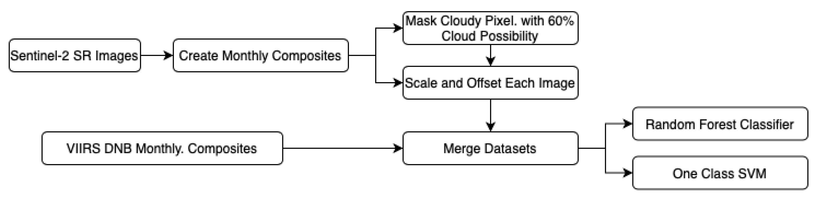
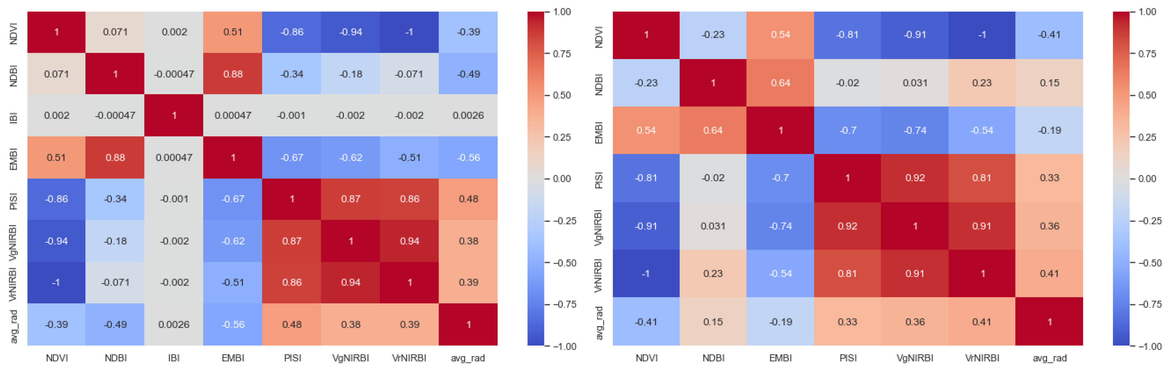
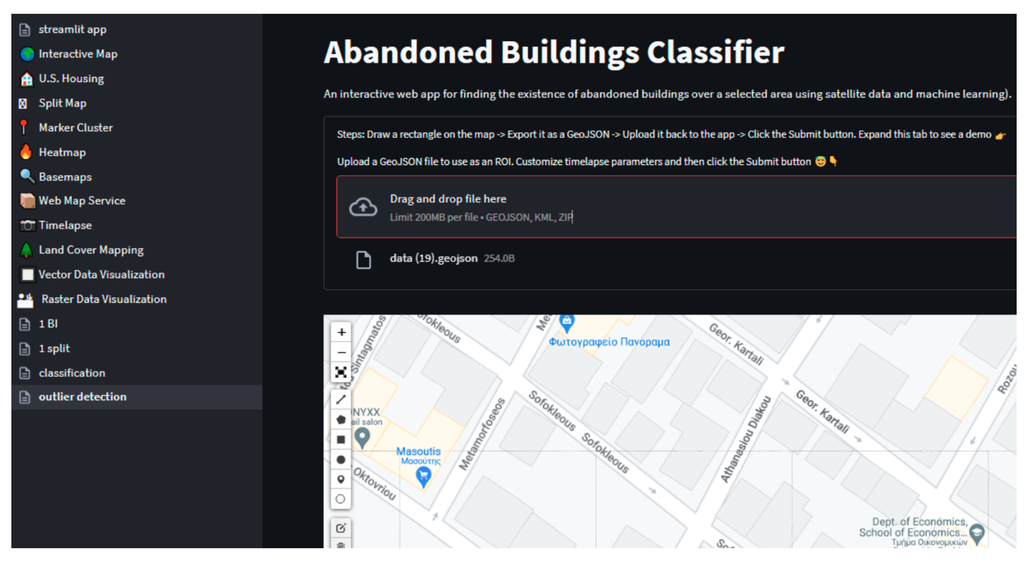
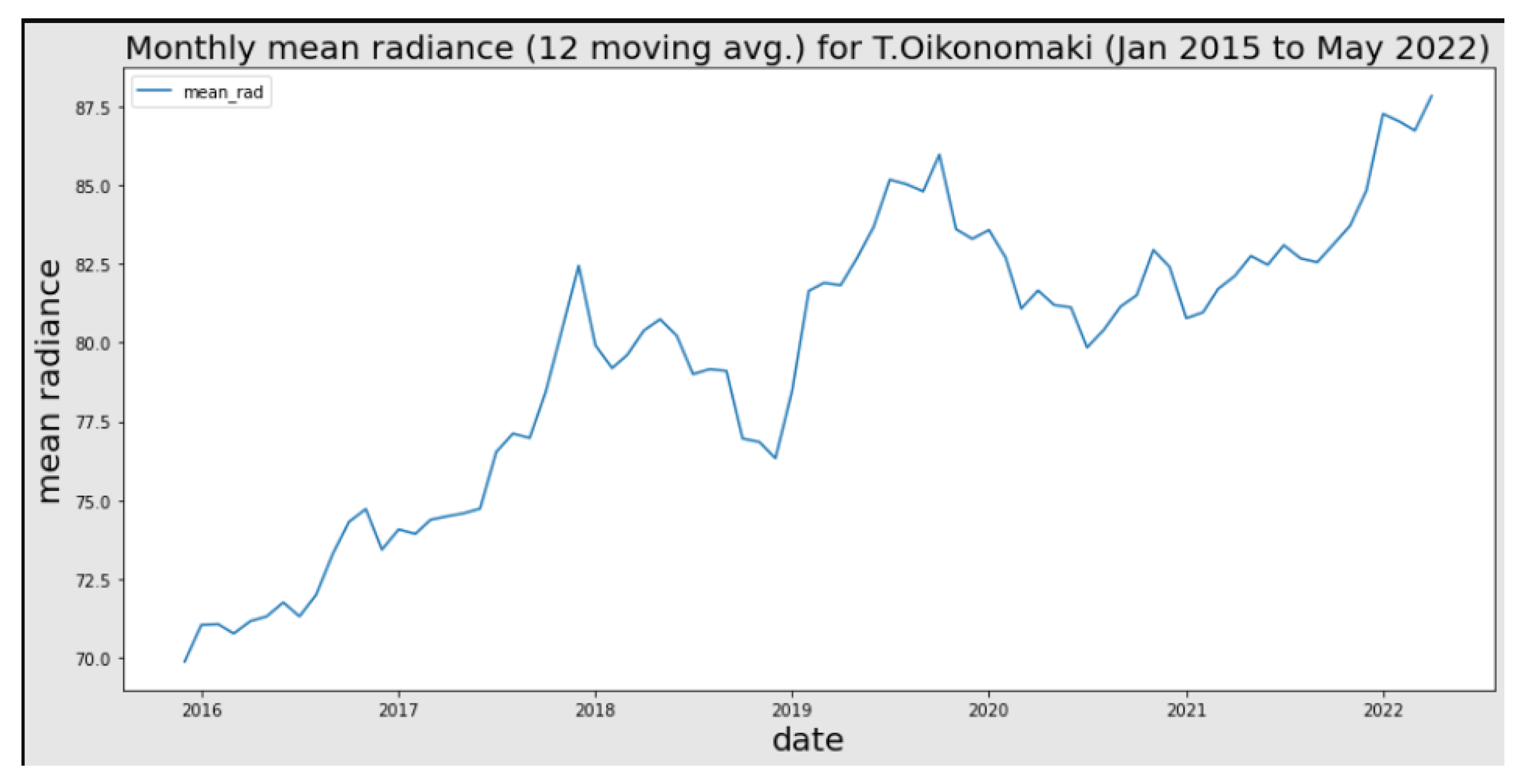
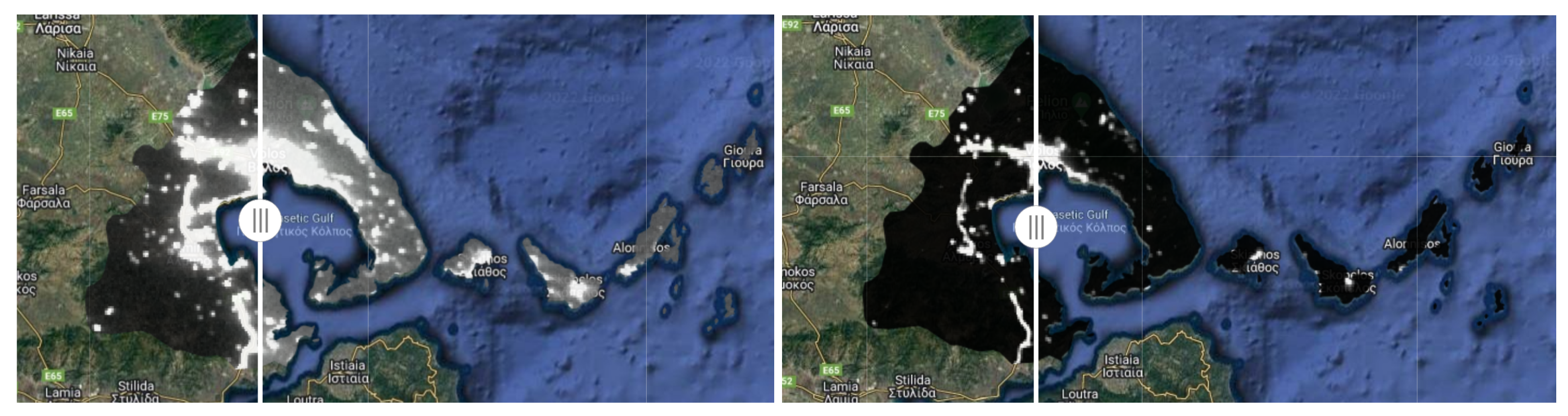
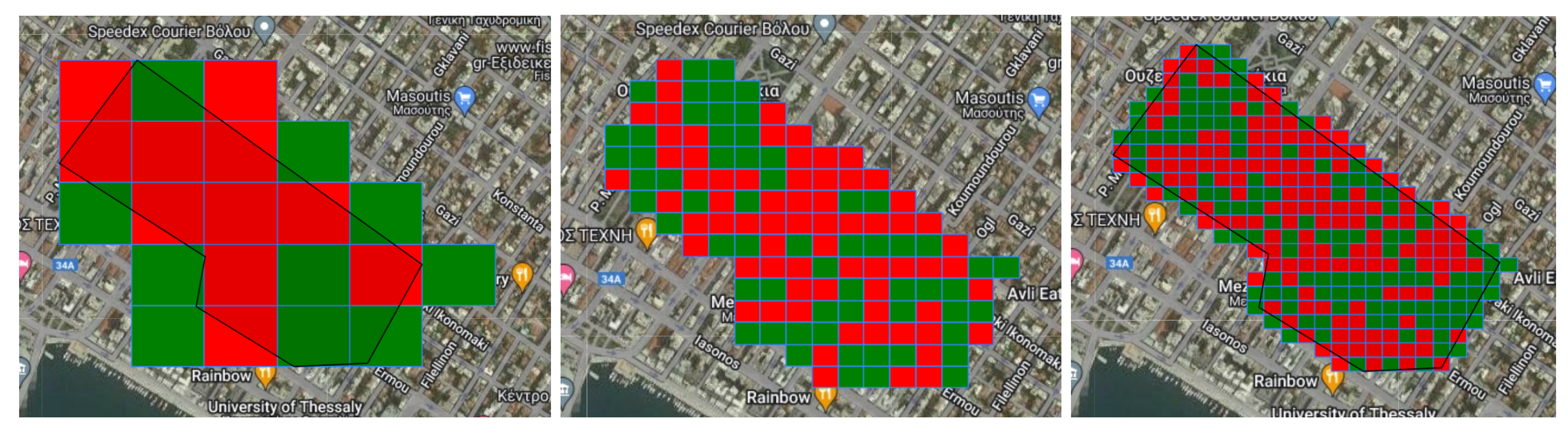
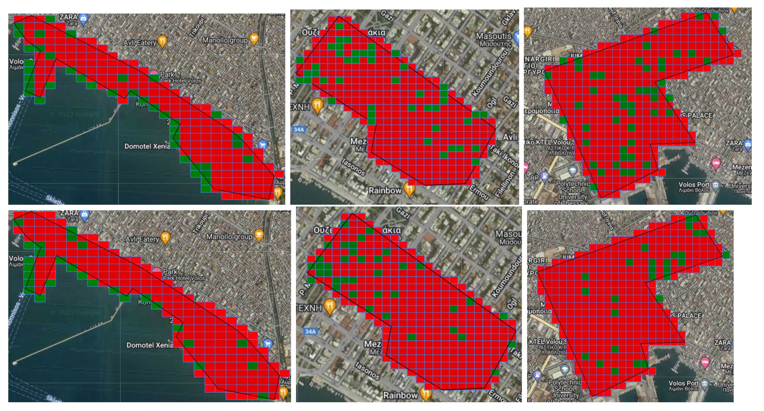
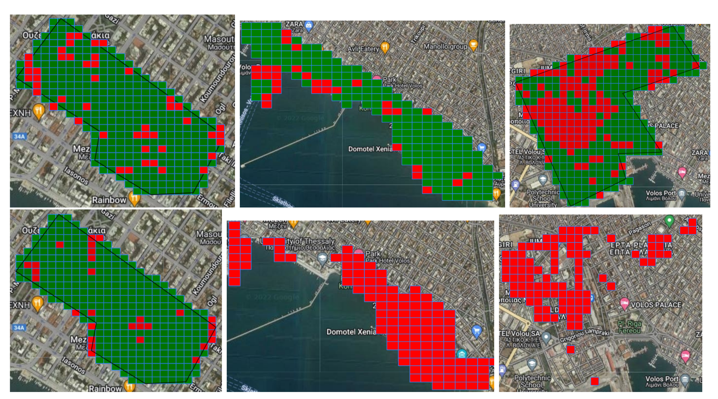
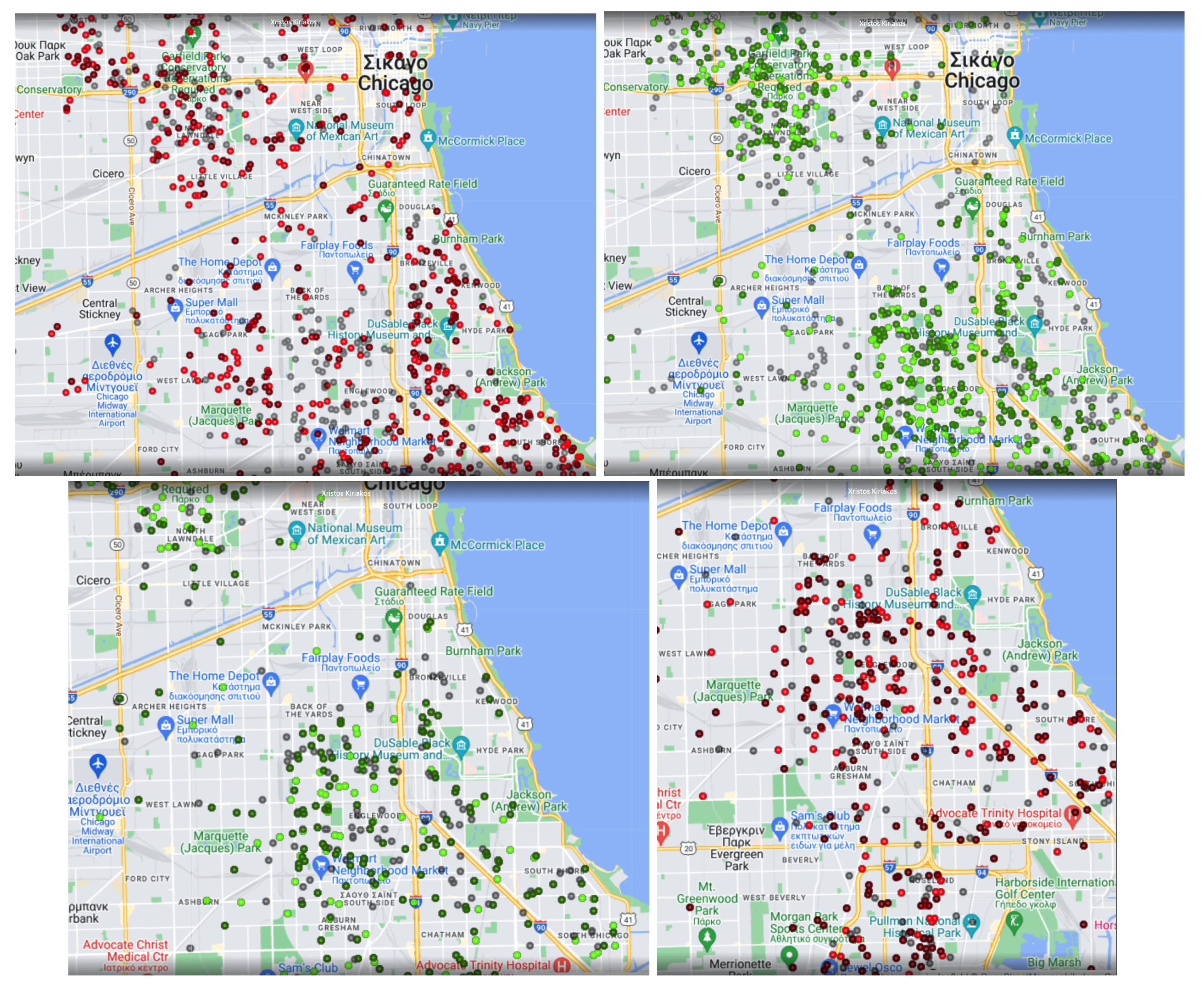
Table 1.
Selected Feature Combinations for Random Forest Experiments.
| Features | Parameters | RF Accuracy | |
|---|---|---|---|
| Max Depth | # of Estimators | ||
| NDVI, NDBI | 20 | 400 | 0.663% |
| NDVI, NDBI, Average Radiance | 20 | 350 | 0.681% |
| VgNIRBI, Average Radiance | 20 | 600 | 0.666% |
Table 2.
Performance comparison for the Convolution Neural Network and the Time Series Forest Classifier for the city of Chicago dataset.
Table 2.
Performance comparison for the Convolution Neural Network and the Time Series Forest Classifier for the city of Chicago dataset.
| Classifier | Accuracy | Precision | F1 |
|---|---|---|---|
| Convolution Neural Network | 0.641148 | 0.563805 | 0.409708 |
| Time Series Forest Classifier | 0.607582 | 0.609809 | 0.594830 |
Disclaimer/Publisher’s Note: The statements, opinions and data contained in all publications are solely those of the individual author(s) and contributor(s) and not of MDPI and/or the editor(s). MDPI and/or the editor(s) disclaim responsibility for any injury to people or property resulting from any ideas, methods, instructions or products referred to in the content. |
© 2023 by the authors. Licensee MDPI, Basel, Switzerland. This article is an open access article distributed under the terms and conditions of the Creative Commons Attribution (CC BY) license (https://creativecommons.org/licenses/by/4.0/).
Share and Cite
MDPI and ACS Style
Kyriakos, C.; Vavalis, M. Business Intelligence through Machine Learning from Satellite Remote Sensing Data. Future Internet 2023, 15, 355. https://0-doi-org.brum.beds.ac.uk/10.3390/fi15110355
AMA Style
Kyriakos C, Vavalis M. Business Intelligence through Machine Learning from Satellite Remote Sensing Data. Future Internet. 2023; 15(11):355. https://0-doi-org.brum.beds.ac.uk/10.3390/fi15110355
Chicago/Turabian StyleKyriakos, Christos, and Manolis Vavalis. 2023. "Business Intelligence through Machine Learning from Satellite Remote Sensing Data" Future Internet 15, no. 11: 355. https://0-doi-org.brum.beds.ac.uk/10.3390/fi15110355
Note that from the first issue of 2016, this journal uses article numbers instead of page numbers. See further details here.