1. Introduction
Economic and environmental sustainability analyses, also in conjoint applications, are recognized to be a fundamental support in decision-making among alternative projects characterized by technical options. These projects can be differentiated by diverse components. This is demonstrated by the wide international literature on the topic, and by the recent debate within scientific communities following international regulatory framework and energy-environmental policies, assuming a multidisciplinary research perspective [
1,
2].
ISO 15686:2008 Buildings and constructed assets—Service-life planning, part 5—Life-Cycle Costing [
3] indicates life cycle cost analysis (LCCA) as a tool for defining preferable projects according to the economic sustainability viewpoint, through global cost calculation [
4]. In recent applications, the LCCA approach is extended towards the economic-environmental sustainability of projects, through the calculation of a conjoint economic-environmental performance indicator [
5].
A crucial step in LCCA applications is the cost-estimating phase, developed through a preliminary activity for defining the life cycle cost estimates (LCCEs), as illustrated in the US Department of Energy (DOE) handbook guidance [
6]. The complexity in defining LCCEs is due to the presence of risk and uncertainty as “structural components” in input data, and, consequently, in the following LCCA applications. As proposed in previous studies, flexibility has to be introduced during input estimates, by means of deterministic approaches such as sensitivity analysis [
5]. The limits of the deterministic approach lead to the consideration of the potentialities of a probabilistic approach, as illustrated in [
7] in which probability analysis is proposed to introduce risk and uncertainty in LCCEs and LCCA, by modeling “critical cost items” in terms of their probability distributions. Specifically, a “hybrid” deterministic-probabilistic methodology is proposed to simultaneously model uncertainty in critical input cost items and uncertainty in relation to variables affected by uncertainty over time (e.g., technological components with uncertain durability).
As stressed in the mentioned study [
7], when modeling the durability of technological components the uncertainty is twofold: on one side, uncertainty affects the estimation of cost items (for example, the cost amount for maintenance/adaptation/replacement of components); on the other side, risk and uncertainty affect the building components service life estimation. In the study, the service lives of two alternative technological components are deterministically expressed through different lifespans. These lifespans correspond to different numbers of periods over the project time horizon. The main criticality is due to the deterministic nature of the input data related to lifespans: The possible variability of these variables in the system is not completely considered, with important consequences for decision-makers involved in the process.
From the discussion on the results of the mentioned step of research, it emerges that facing a twofold level of uncertainty implies difficulties during the LCCA modeling phase, and during the critical input calculation preliminary to the LCCA application. Starting from these premises, in the present research it is assumed that the durability of components and their relative service lives can influence both the model construction and, consequently, the model results, and, even more important according to an estimative viewpoint, are able to influence the estimated residual values.
The aim of this work is to present a methodological proposal to treat uncertainty not only related to the variability of the cost items amount, but also related to the service lives of the project technical components, or their durability, by introducing flexibility over time. The methodology proposed assumes the methodological framework presented in the above-mentioned study, and develops the input modeling through the Factor Method (FM) as illustrated in ISO 15686:2008 and in the recent literature on the topic. Furthermore, a step forward is presented: The stochastic approach to the FM for estimating the service lives of the components considered, in terms of probability distribution functions (PDFs), is proposed. Subsequently, the introduction of the estimated PDFs into the LCCA model is proposed. Coherently, the LCCA output is expressed through a PDF, by calculating the stochastic global cost distributions for two different options.
As a case study for the application, two different glass façades of an office building located in Turin (Northern Italy) are considered, based on two previously compared [
5,
7] alternative technical components—a timber frame and an aluminum frame—maintaining data and conditions.
The application demonstrates that the stochastic estimates of service lives, modeled through a stochastic approach to the FM application, are able to perturb significantly the LCCA model output. Results give full evidence of the capacity of lifespan variables to affect the global cost calculation, overcoming the effects of environmental elements—which have been explained in recent applications—and even the financial ones, in contrast with the consolidated empirical evidence. Furthermore, the study shows that beta and gamma distributions are preferable when introducing flexibility over time during the building construction processes, confirming the literature on the topic. The methodology adopted demonstrates to be an effective tool when in presence of alternative investment options, enforcing the decision-making process towards economic-environmental preferable solutions in a temporal perspective.
The paper is articulated as follows: In
Section 2, a literature and scientific background on the topic is presented. In
Section 3, the methodology is illustrated. In
Section 4, the case study is mentioned. In
Section 5, the results of the methodology application are presented and discussed.
Section 6 concludes the paper.
2. Literature Background
In recent decades, a wide literature has been produced on economic-environmental sustainability, stemming from international regulatory frameworks and guidelines. Energy and environmental policies are translated into methodological addresses, based on life cycle thinking and on circular economy principles. A vast debate has ensued, involving a multidisciplinary spectrum of scientific competences, paying special attention to the construction sector as it is responsible for the largest part of negative environmental externalities and energy consumption.
The economic viewpoint is central in the methodologies proposed by the norms and in the deriving literature, shifting the attention towards an economic-energy-environmental concept of sustainability, and focusing also on the potential consequences for real estate market dynamics and transaction prices [
8,
9,
10,
11,
12].
The “Real Estate Appraisal and Economic Evaluation of Projects” disciplinary research addresses a particular interest towards the international standards ISO 15686:2008, specifically part 5—“Life Cycle Costing”. This is one of the main reference documents for the development of recent studies and applications of LCCA, with some other founding documents [
13,
14,
15].
There is a focus on decision-making in the early design stages, in the presence of risk and uncertainty in input data; studies explore the use of risk analysis, also in conjunction with LCCA [
16,
17,
18,
19,
20,
21,
22,
23,
24,
25,
26,
27]. Furthermore, special attention by researchers is paid to the study of the preferable PDFs both in the case of stochastic input variables such as cost items (in many cases a triangular type of PDF is suggested), and in the case of stochastic variables referring to time, as, for example, cost items referred to the construction phase and affected by uncertainty over time (in this case, beta and gamma distributions are explored) [
22,
28,
29,
30,
31].
Moreover, other parts of the series ISO 15686:2008 are considered, being directly linked to issues faced in this work:
ISO 15686-1:2000, Building and constructed assets—Service Life planning—Part 1: General principles [
32];
ISO 15686-2:2001, Building and constructed assets—Service Life planning—Part 2: Service Life prediction procedures [
33];
ISO 15686-7:2006, Building and constructed assets—Service Life planning—Part 7: Performance Evaluation for Feed-back of Service Life data from practice [
34];
ISO 15686-8:2008, Building and constructed assets—Service Life planning Part 8: Reference Service Life and Service Life estimation [
35];
UNI 11156-3: 2006, Valutazione della durabilità dei componenti edilizi. Metodo per la valutazione della durata (vita utile) [
36].
As emerges from the ISO 15686-1:2000, the valuation of service life in the early design stages can be supported by the FM. The “simple” FM is described by several authors on the basis of the norms ISO 15686—part 1:2000 and UNI 11156:2006. Davies and Wyatt [
37] give a clear presentation of the model, in combination with the cluster mapping technique, focusing on the practical aspects in applying the ISO 15686 methodology in the building sector.
The FM presents a very simple methodological framework; meanwhile, it is affected by subjectivity. Furthermore, it is necessary to support standardized and scientifically validated methods for durability estimation, on the bases of a limited number of reference service lives (RSLs) considered as reference values. RSLs prediction is considered as a fundamental step in the literature, even if, in the case of a building component, it is very difficult to estimate: the behavior of the component over time must be foreseen. Nevertheless, service life prediction is fundamental for applying economic-energy-environmental sustainability valuation approaches—for example, life cycle assessment (LCA) and LCCA—and maintenance cost estimation activities, as in the present study. These approaches are founded on project life cycle prediction and on project sustainability, according to the building products durability requirements expressed by the recent EU guidelines and regulations. RSL must be defined in relation to a concrete and specific context (e.g., use, or specific technological configurations), and considering that a low variation in the input can cause a relevant variation in the output. According to the authors, the RSL is one of the most difficult variables to quantify, through:
Expert opinions and experiences, and knowledge of component behavior (in similar conditions);
Scientific research, technological information by producers, laboratory tests, and statistical analysis, etc.
The scientific literature presents different approaches for building construction service life estimation. A general distinction is made among [
38,
39]:
Deterministic approaches, for example, the “simple” FM, mathematically simple but not very affordable;
Probabilistic approaches, very affordable and detailed, but very expensive in terms of input data required and calculation;
Engineering approaches, for example, the engineering of the FM, able to maintain the simplicity of the method but reinforcing its affordability.
Assuming the difficulties in predicting service lives of building components, due to the high sensibility to even very low perturbations in the context of analysis, and assuming the potential degree of subjectivity of the simple FM, different approaches are proposed in the literature in order to manage the uncertain input estimates and/or develop advanced methodological steps for specific analysis [
40,
41,
42].
For example, the “Group of Durability” of the Politecnico di Milano, Italy, proposes to solve the FM through the engineering approach, based on “grids” defined on a performance basis [
43,
44]. In these studies, the grids are based on the characteristics of the building component able to influence its durability. Through this “performance approach” it is possible to reduce the subjectivity of the FM. Operatively, the performance approach is solved by using the corrective factors of the RSL, determined through experimentations, laboratory tests, simulations, and so on.
In each factor grid, variables that can significantly condition the components duration are considered, on the basis of seven factors, as indicated by the ISO 15686—part 8. Examples of an advanced FM and factor grids are presented in [
43]. Each factor is divided into a set of sub-factors, which put in evidence the elements capable of influencing the degradation process, accelerating, or diminishing the component performance, and to influence the durability of the single component/entire building. The factor grid construction is devoted to a group of experts, in order to lower, as much as possible, the subjectivity; the grid definition is based on the following main steps:
Building component description and context variability through the factors of the FM;
Relevant factors individuation, through scientific literature or experimental tests.
The authors point out that, being a presentational approach, the building is considered as a system of performances; the factor grid may be considered as a way to represent these performances over time. This implies the development of a performance analysis over time and critical value identification for each variable (critical performances). The minimum critical value calculated among all the considered variables represents the service life.
In developing the method, it must be considered that the possible selected factors and sub-factors for the service life estimation can be affected by uncertainty in the input data. For this reason, studies propose a stochastic approach to the FM; even if difficult, stochastic methods are very effective to treat uncertainty: The stochastic input parameters are considered as “modifying factors” in service life prediction. The authors [
45], presenting an application of the stochastic approach to the FM in the case of durability of rendered façades, sustain that the degradation process of building materials occurs as a stochastic phenomenon and, for that reason, deterministic models are not able to treat the random nature of degradation phenomena and buildings’ performances. The factors that can influence the durability are expressed by probability distributions and each option is associated to an ESL, through a probability distribution with an associated confidence interval. More precisely, each factor/sub-factor must be evaluated for each case and can be quantified with specific methods, including the distribution functions definition [
46].
3. Methodological Background
This work assumes the methodology illustrated in two previous studies, as mentioned in the introduction [
5,
7].
The first study proposes a “simplified” application of LCCA to identify the preferable solution between different technological options oriented at reducing environmental and economic impacts (including investment capital, maintenance, and end-of-life costs). The Standard ISO 15686-5:2008 [
3], the Standard EN 15459:2007 [
4], the relative Guidelines accompanying Commission Delegated Regulation (EU) No 244/2012 [
47], following the Directive 2010/31/EU—EPBD recast [
48], are followed to develop the methodology and the global cost calculation. The global cost calculation is expressed through a “synthetic economic-environmental indicator” including monetized environmental impacts (embodied energy—EE and embodied carbon—EC), disposal/dismantling costs and residual value. Two different technologies (components) are compared for selecting the most viable solution. The results of LCCA application are expressed through the quantitative indicator net present value. The application is implemented considering the same energy performance for each design option; there is a focus on the differences in the building components maintenance costs, and the end of life stage. Cost items related to the environmental impacts (monetized) are summed to global cost. Formally, the approach is resolved according to Equation (1):
where: C
GEnEc is the life cycle cost including environmental and economic indicators; C
I the investment costs; C
EE the costs related to embodied energy; C
EC the costs related to the embodied carbon; C
m the maintenance cost, C
r the replacement cost; C
dm the dismantling cost and C
dp the disposal cost; V
r the residual value; t the year in which the cost occurred and N the number of years of the entire period considered for the analysis; r the discount rate. A deterministic sensitivity analysis concludes the work.
In the second study, risk and uncertainty are included in the LCCA application, distinguishing between “uncertainty in cost-estimating”, expressed in terms of life cycle cost estimate (LCCEs) and “uncertainty in technical performance” referred to the life cycle cost analysis application (LCCA) [
6]. A formal quantitative risk analysis is resolved through the probability analysis approach (see the references mentioned in
Section 2).
A sensitivity analysis is used as the first step for selecting the input variables to be modeled through the probability analysis. In fact, through sensitivity analysis it is possible to identify the parameters to which the model predictions are most sensitive, or, in other terms, it allows the identification of the input distributions that are significant in determining the values of output variables. Probability analysis, in turn, is solved through the simulation method, producing probability functions for the most relevant (stochastic) variables and measuring their functional forms with the support of random number generation, and then by isolating and quantifying the marginal contribution of each variable. Notice that, in this context, stochastic variables are used to represent the variability in input and output values, when the presence of uncertainty requires the use of a range of values instead of point values. The ranges of values are expressed statistically through probability distribution functions. The functions are defined by means of numerical methods, based on the generation of random number sequences, and by testing out the randomness and validity of the starting conditions, and then by the extraction of sampling values for the reproduction of the variables (random variates).
Coherently, the model output is calculated in terms of stochastic global cost through the following Equation (2):
where
is the life cycle cost, including environmental and economic indicators expressed in stochastic terms;
is the stochastic investment costs;
is the stochastic costs related to embodied energy;
is the stochastic costs related to the embodied carbon;
is the stochastic maintenance cost,
is the stochastic replacement cost;
is the stochastic dismantling cost;
is the stochastic disposal cost; V
r is the residual value; t is the year in which the cost occurred; N is the number of years of the entire period considered for the analysis (representing the time required to renew and retrofit the building according to the regulations on energy consumptions and to the evolving functional requirements); and
is the stochastic discount rate. Notice that the residual value V
r is due to the difference between the entire period of the analysis and the specific service life of components object of the study; simplifying, the residual value is considered as a deterministic input. An empirical modality is adopted by defining three different lifespan scenarios, representing the possible temporal variability of the components. As a consequence, three different residual values are obtained. Notice that the determination of possible temporal variability of components is the most crucial aspect of the analysis, and its rational quantification will be the focus of the present work.
In the present work, a methodological step is proposed to model lifespans as stochastic input variables, by using the stochastic approach to the FM. This can be considered an advanced modality based on the “simple” FM.
Formally, the ISO 15686 presents a “generic model”, in which FM is used to estimate the service life of a building component by multiplying its RSL by a set of factors that can potentially influence the durability, related to specific conditions, as in the following Equation (3):
where ESL represents the estimated service life of a component, RSL represents the reference service life, A represents the quality of materials and components, B the design level, C the work execution level, D the indoor environment conditions, E the outdoor environment conditions, F the in-use conditions, G the maintenance level. The equation presented is a general framework, and each factor—defined for each specific application—is evaluated through the distribution functions definition.
As an assumption, due to the methodological purpose of the study, the values of the factors are not quantified on the basis of laboratory experiments on specific components, but on hypothesis based on data deducted by the literature.
According to a “technological” viewpoint, it would be advisable to individuate a set of sub-factors related to each factor in the Equation (3); these specific sub-factors, linearly combined, could represent the synthetic factors indicated by literature. In this work, a simplified solution is adopted, by assuming a hypothesis of the factors’ entity, in relation to the following qualitative considerations: Use conditions; use environment; component quality. The selection of the specific sub-factors is based on the literature on the topic.
The generic equation is adopted and, in our case, all factors are considered as stochastic input, exception for RSL (point data), as in Equation (4):
where
stands for stochastic estimated service life of a component, RSL represents the reference service life,
represents stochastically the quality of materials and components,
represents stochastically the design level,
represents stochastically the work execution level,
represents stochastically the indoor environment conditions,
represents stochastically the outdoor environment conditions,
represents stochastically the in-use conditions,
represents stochastically the maintenance level.
The stochastic ESL calculation permits to complete the Equation (2) as follows Equation (5):
where
is the life cycle cost, including environmental and economic indicators expressed in stochastic terms;
is the stochastic investment costs;
is the stochastic costs related to embodied energy;
is the stochastic costs related to the embodied carbon;
is the stochastic maintenance cost,
is the stochastic replacement cost;
is the stochastic dismantling cost;
is the stochastic disposal cost;
is the stochastic residual value; t is the year in which the cost occurred; N is the number of years of the entire period considered for the analysis; and
is the stochastic discount rate. Notice that, unlike in the Equation (2), the residual value is considered here as a stochastic input, being obtained through the stochastic ESL calculation.
Summing up, to resolve Equation (5) the same steps described in the previous work are proposed [
7], with the exception of the calculation of the stochastic residual value
solved by applying the stochastic FM. Note that there is a substantial difference in respect to the workflow adopted in the previous research. In the previous research, the time variable is modeled by introducing point estimates and by creating deterministic scenarios (all the other variables are stochastic). In this work, the point data is substituted by a variable service life, through a calculated PDF by means of the stochastic FM.
In detail, the steps of the analysis performed are the following:
Determination of the estimated service life through the stochastic approach to the Factor Method
- −
Step 1: Reference service life assumption. In this first step the RSL of the component is defined, through estimates based on empirical laboratory tests, generally developed by the manufacturers;
- −
Step 2: Individuation of the factors for FM application, on the basis of the literature on the topic and on a hypothesis based on data deducted by the literature; preliminary hypothesis for factor values determination (according to Equation (3)) and individuation of alternative scenarios;
- −
Step 3: individuation of the distribution type and PDFs calculation through Monte Carlo Method (MCM). This step is developed through iteration and sampling, according to the numerical methods;
- −
Step 4: Stochastic estimated service life calculation, through the MCM (according to Equation (4)), on the basis of the stochastic factors defined above;
- −
Step 5: Best-fit distribution calculation to obtain a PDF related to the EL. The preferable distribution function (best fit) is deducted by a ranking of distributions based on the results of statistic measures calculation (Chi-squared, Kolmogorov-Smirnov, Anderson-Darling, Root-Mean Squared Error), used for testing how the distribution fits the input data and to test the confidence on the distribution functions representativeness;
Introduction of stochastic service lives input data in life cycle cost analysis
- −
Step 6: Recalculation of the results of LCCA using the PDF of the EL as input data for the resolution of the Equation (5);
Calculation of LCCA results and final considerations
- −
Step 7: Defining the best-fitting distribution function for the output values (following the Step 5 procedure) calculated in Step 6 and results interpretation.
5. Application and Results
The methodology illustrated in
Section 3 is applied in the case study mentioned above. The results of the simulations performed through the software @Risk (by Palisade Corporation, Ithaca, NY, USA, release 7.5) are illustrated in the following subsections.
5.1. Determination of the Estimated Service Life through the Stochastic Approach to the Factor Method
As the first step, a RSL is assumed. In this case, a RSL of 20 years is adopted for both options (assuming the manufacturer’s indications as in the previous work, and making reference to the average service life for the considered class of components).
As the second step, the factor values are determined and grouped in three main “families”, according to the following general and preliminary hypothesis (as mentioned before, considering indicative values deducted from the literature):
Factors related to inherent quality characteristics (quality of components, design level, and work execution level): During the design and installation phase no relevant differences are detectable as respect the manufacturer’s indications. In other terms, no significant deviation is expected as respect the RSL (Factor values 1);
Factors related to environment (indoor environment and outdoor environment): A reduction in respect to the RSL is expected (Factor values less than 1), due to more severe environmental conditions in respect to the RSL ones (outdoor conditions worse than indoor conditions). Notice that the building is located in Turin’s suburban area, devoted to commercial-tertiary use, and for these reasons it is reasonable to foresee a reduction in RSL. Furthermore, a reduction in relation to the Factor E value is foreseen more significant for timber frames than aluminum frames, assuming that external pollution has more effect on timber than on the aluminum;
Factors related to operating conditions (in use conditions and maintenance level): An increase in respect to the RSL is expected (Factor values higher than 1), due to the foreseen presence of better operating conditions in respect to the RSL ones. In fact, a high level of quality of building and functions to be inserted are prefigured by the project.
It must be considered that the values indicated in
Table 1 are finalized to present a plausible picture of a concrete scenario, although they are not based on specific laboratory experiments or empirical evidence.
Furthermore, in the second step, two different scenarios are also prefigured, assuming more or less impactful Factors D, E, F and G:
Low-impact factor scenarios: a minor deviation from RSL is hypothesized, in reduction and increase (minor impact of environmental factors produces a reduction, and operative an increment);
High-impact factor scenarios: a greater deviation from RSL is hypothesized, in reduction and increase (higher impact of environmental factors—reduction and operative—increment).
Consequently, in the third step the factors are made stochastic, as previously mentioned, through the support of the Monte Carlo method simulation; notice that:
The factors can be expressed through a specific PDF. According to the literature, the lognormal distribution is the most frequently adopted and, in our case, the lognormal distribution is assumed for representing the factor’s values;
The lognormal distribution reflects the greatest probability that the component could have a service life lower than the RSL. Distribution curves are of the lognormal type, are skewed to the left, with maximum probability given by peaks of the curves. The right side of the distribution reveals also a low probability of service life values higher than RSL.
Table 2 and
Table 3 presents factor values and probability distributions calculated for the low and high scenario respectively.
The fourth step of the analysis consists of the stochastic estimated service life calculation, through the MCM, on the basis of the factors defined above.
Figure 2 and
Figure 3 present the PDFs, the relative cumulative functions, and statistics, for both scenarios (low and high).
Note that the E
L calculation is obtained by Equation (4). The calculated results, presented in
Figure 2 and
Figure 3, must be represented in the corresponding best-fit distribution curve in order to be modeled as input data into the LCCA application.
As the fifth step, it is now necessary to obtain a PDF related to the EL.
As shown in
Figure 4 and
Figure 5, the Pearson seems the best-fitting distribution (the lognormal results are the second best distribution). The parameters of the Pearson distribution are indicated in the figure; the different confidence intervals and distribution statistics are also indicated. Pearson is the best fit in both scenarios (low and high), in the case of timber and aluminum frames.
The Pearson distribution is obtained through the best-fitting procedure mentioned in
Section 3. Particularly, for example, in the case of the timber frame low-impact scenario, the Chi-squared statistic value amounts to 163.65 for the Pearson distribution, which is the preferable result in the ranking. In the same example, the lognormal distribution, with a Chi-squared value of 315.47, is the second one in the ranking.
The PDFs obtained and represented in
Figure 4 and
Figure 5 are introduced as input data into the LCCA application, as illustrated in the following sub-section.
5.2. Introduction of Stochastic Service Lives Input Data in Life Cycle Cost Analysis
The sixth step consists of the recalculation of the results of LCCA using the PDF of the E
L as input data for the calculation as in the Equation (5). Coherently with the previous study, the main assumptions about input data are illustrated in
Table 4.
Notice that the analysis is conducted on the elements with the same energy performance in order to identify the preferable component from a sustainability viewpoint. As in the previous application, account is taken for the embodied energy (EE) and the embodied carbon (EC) that the realization implies. EE and EC are considered in relation to both the service life of the components (in terms of maintenance costs, replacement costs, etc.) and to the end-of-life phase, focusing on the environmental impacts in the construction and execution phases.
In
Table 5 input data and probability distribution values are reported for the low scenario (for example).
Notice that the two Pearson distributions are inserted in the table. The other inputs are triangular type distributions.
Figure 6 depicts the outputs obtained through the MCM simulation, for timber frame and aluminum frame, for briefness only in relation to the low scenario.
In
Figure 7, for low- and high-impact factor scenarios for timber and aluminum frames, the input variables are ranked by their effect on output mean (graphically expressed through tornado graphs).
As evidenced in
Figure 8, the Spearman correlation coefficients calculated reveal the high impact of lifespan on the general results (the longest bar). The Spearman correlation coefficients are calculated for determining the correlation between the output value (stochastic global cost) and the samples for each input distribution. It is a value between −1 and 1, representing the desired degree of correlation between two variables (global cost and each input data) during sampling. Positive values indicate a positive relation between the variables; negative coefficient values indicate the opposite.
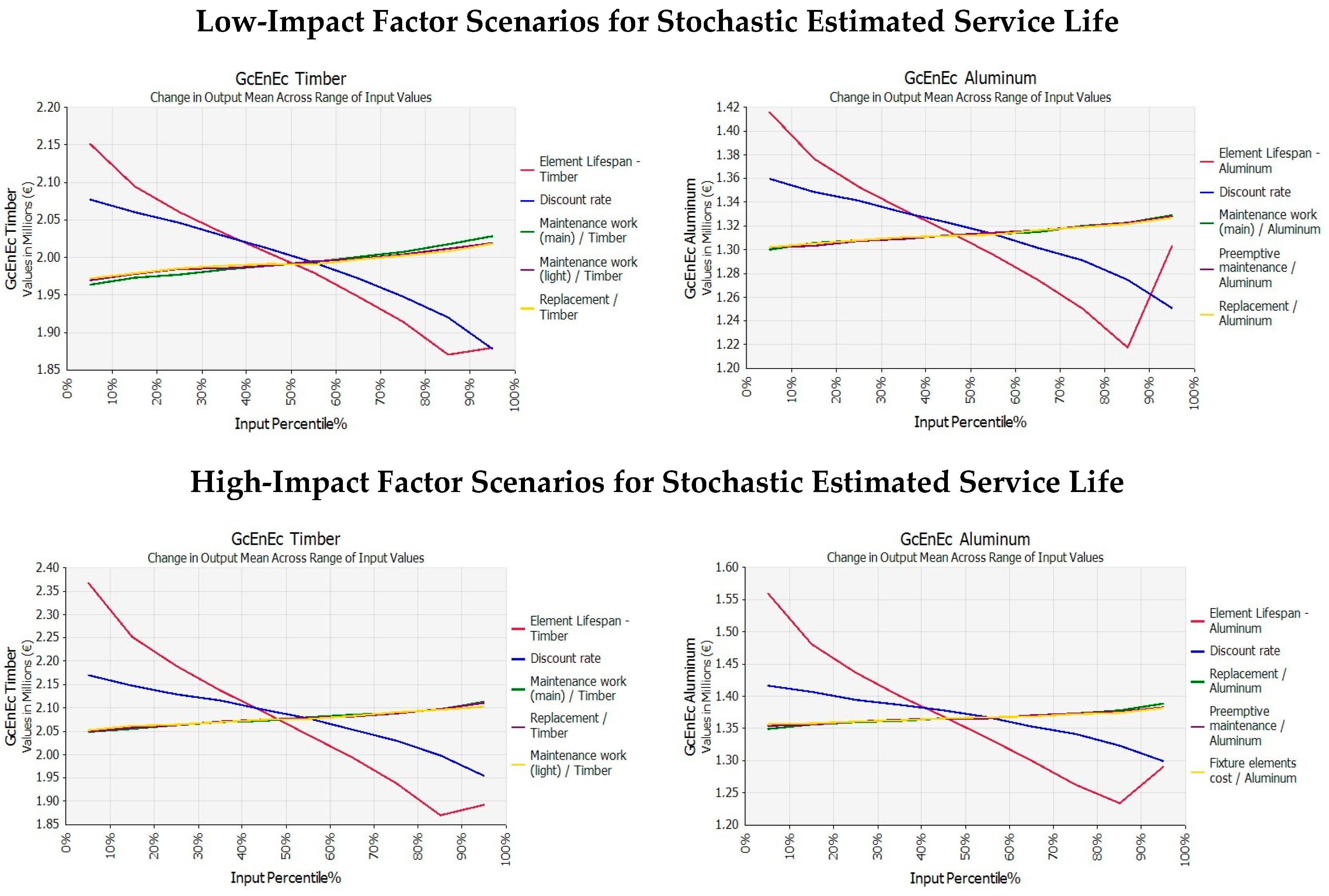
Similarly, the significant influence of lifespan on model output is confirmed by spider graphs (
Figure 9), with the most evident slope. In the previous article, it was not possible to analyze the impact of this specific input data, being considered deterministically. In this application, for both alternative technologies, lifespan represents the variable with the highest perturbation potentiality on LCCA output.
In conclusion, from the analysis emerges that the service life (lifespan), given the assumptions previously illustrated, is the most relevant input factor to the LCCA output calculation, maintaining fixed all the other input elements.
For this reason, it is advisable to recalculate the stochastic global cost as expressed by Equation (5), by introducing the r. The results of the calculation (by MCM simulation) are reported in following sub-section.
5.3. Calculation of LCCA Results and Final Considerations
Concluding the analysis, the simulation output results are compared as reported in
Table 6 and
Table 7, respectively for low-impact factor scenarios for stochastic ESL, timber and aluminum frames, and for high-impact factor scenarios for stochastic ESL, timber and aluminum frames.
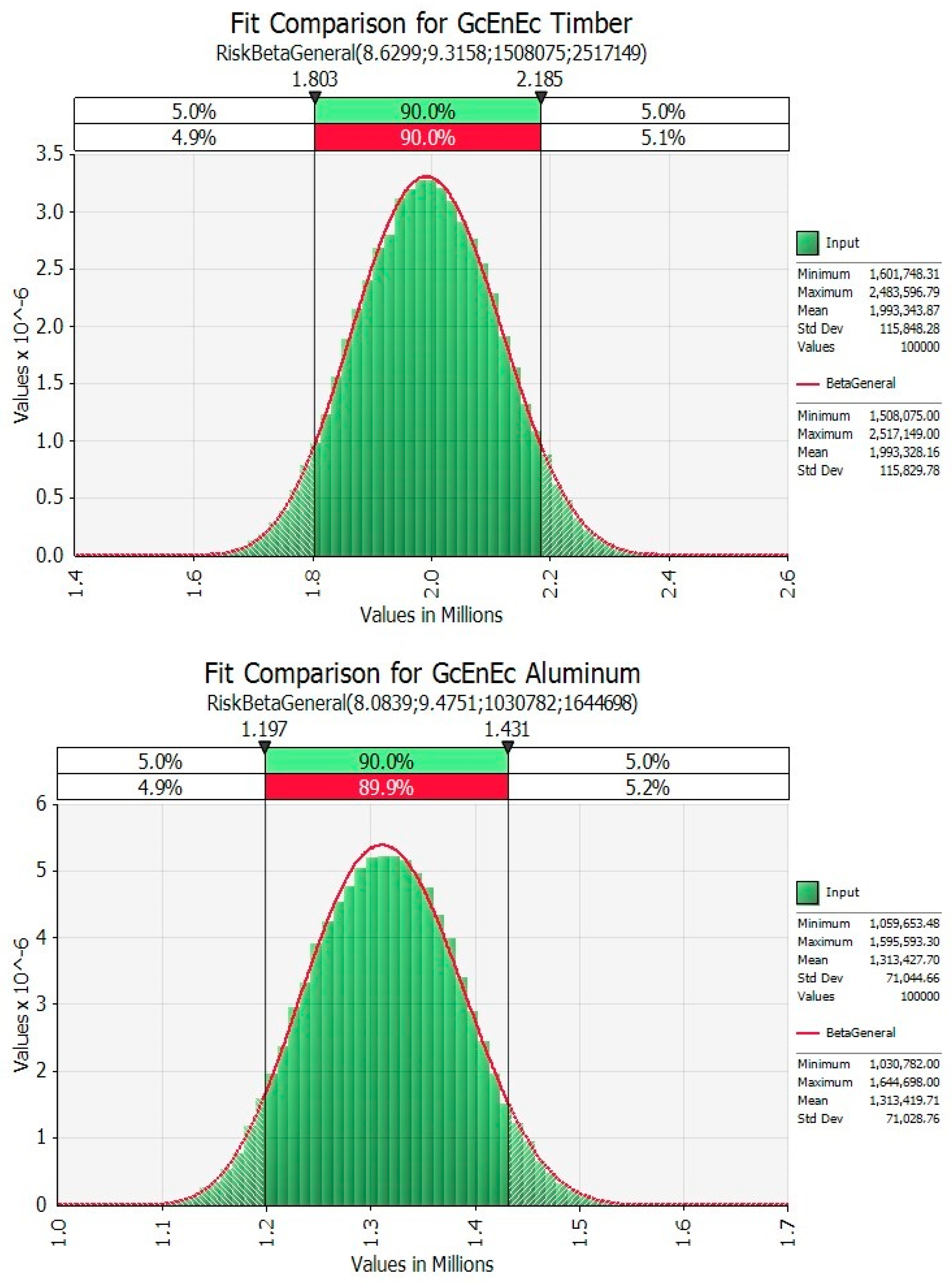
Figure 10 and
Figure 11 conclude the results presentation, with the seventh step, illustrating the best-fit distribution function for the output values above. In the cases of timber frame and aluminum frame low-impact factor scenarios, and timber frame low-impact factor scenarios, the beta distribution results fit best for the stochastic global cost values. Only in the case of aluminum frame high-impact factor scenarios, is the gamma distribution preferable for fitting the values distribution.
This result is perfectly coherent with the literature on the topic, suggesting that, in many cases, the beta and the gamma distributions are preferable for modeling uncertainty in time, by using stochastic variables and introducing flexibility over time during the building construction processes (see the references mentioned in
Section 2).
Lastly, it is worth mentioning that the presence of EL has a reflection also in improving the shape of PDF expressed through triangular type distributions (as a comparison with the previous work reveals).
6. Conclusions
The methodology proposed in this paper has been applied on a case study related to the selection of the preferable solution between two alternative technological components, in economic and environmental terms (a multifunctional building glass façade in Turin, Northern Italy). The same case study has been explored in two previous works of which this paper constitutes a further methodological development.
The economic and environmental sustainability of the project, has been analyzed with a synthetic “economic–environmental indicator”, calculated in terms of a stochastic global cost. In this work the calculation of the stochastic global cost has been implemented by also treating the residual value of the components as a stochastic variable. By assuming the ISO 15686 indications, the Factor Method has been proposed, through a stochastic approach.
The input for the application of the LCCA has been obtained through the application of probability analysis for defining the PDF of relevant cost items, and through the stochastic approach to the FM for modeling the uncertainty in the service life of components (durability).
The results reveal a relevant impact and utility in introducing flexibility in the lifespan of components, shifting from a deterministic to a probabilistic approach.
Considering the results of the regression analyses produced, it emerged that the uncertainty in the lifespan input variable can determine the largest perturbation on the output, in opposition to the frequent relevance of financial variables in long-term valuations such as LCCA applications. Cost items are relatively or poorly significant in the results, as in previous studies. Furthermore, from the study emerges that the beta and gamma distributions are confirmed to be the best fit when introducing flexibility over time during the building construction processes, confirming the literature on the topic.
Lastly, the methodology adopted demonstrates to be an effective tool when in the presence of alternative investment options related to technological alternatives enforcing decision-making in a temporal perspective.
As a conclusion, it must be stressed that the results can support the decision-making processes developed by public authorities and private operators, specifically through the implementation of policies and practices oriented to promote the integration of maintenance, repair, and replacement. In fact, since the early design phases, and during the building construction, a consciousness of the potential effects of the different technological scenarios, when in presence of uncertainty, can help in facing the risks introducing flexibility into the design process. Following the proposed methodology, more extensive experimentations could be developed considering other components or entire building systems, also referring to different building typologies; these could support the definition of policies extending to territorial sub-segments (for example, building districts or typologically homogeneous portions of territory), and are flexible both in respect to the market conditions and to the behavior of the component/system/building over time.


