Remote Sensing Detection of Vegetation and Landform Damages by Coal Mining on the Tibetan Plateau

 , ,
, ,
Abstract
:1. Introduction
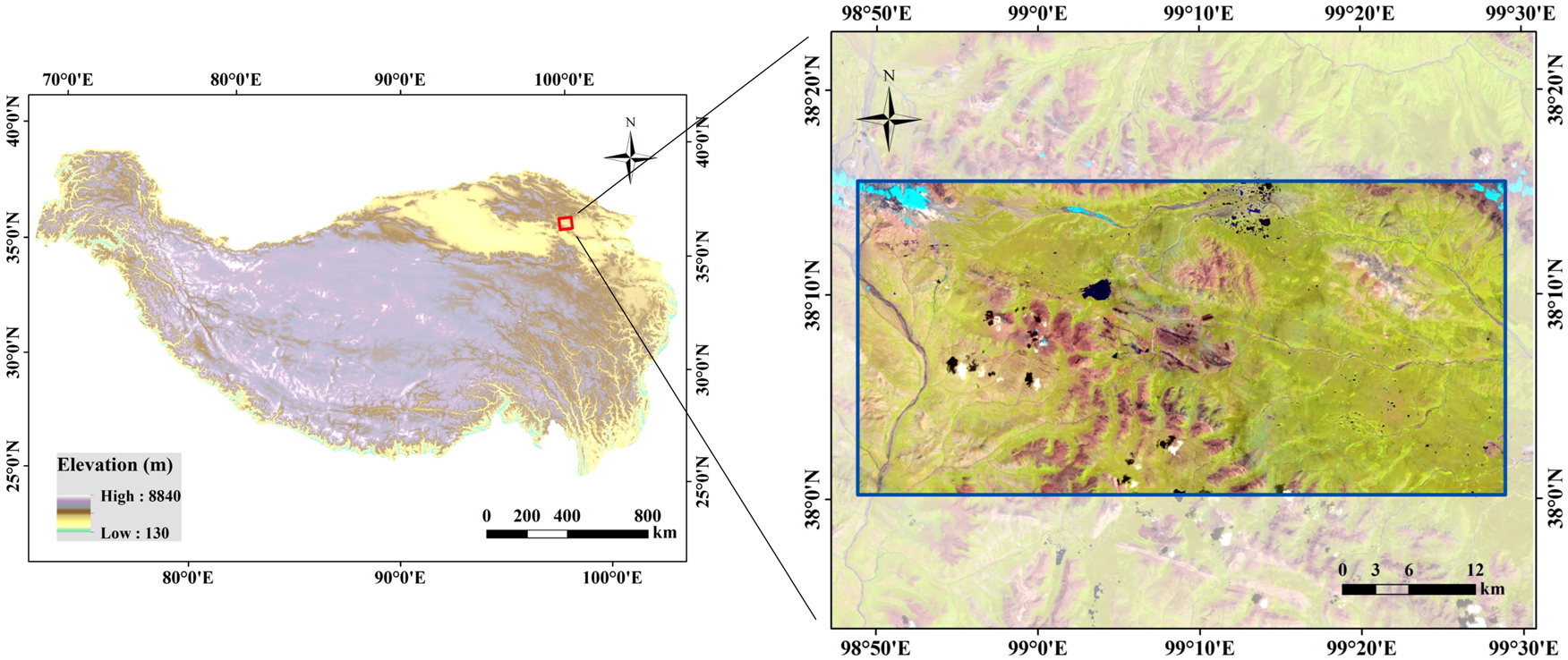
2. Study Area
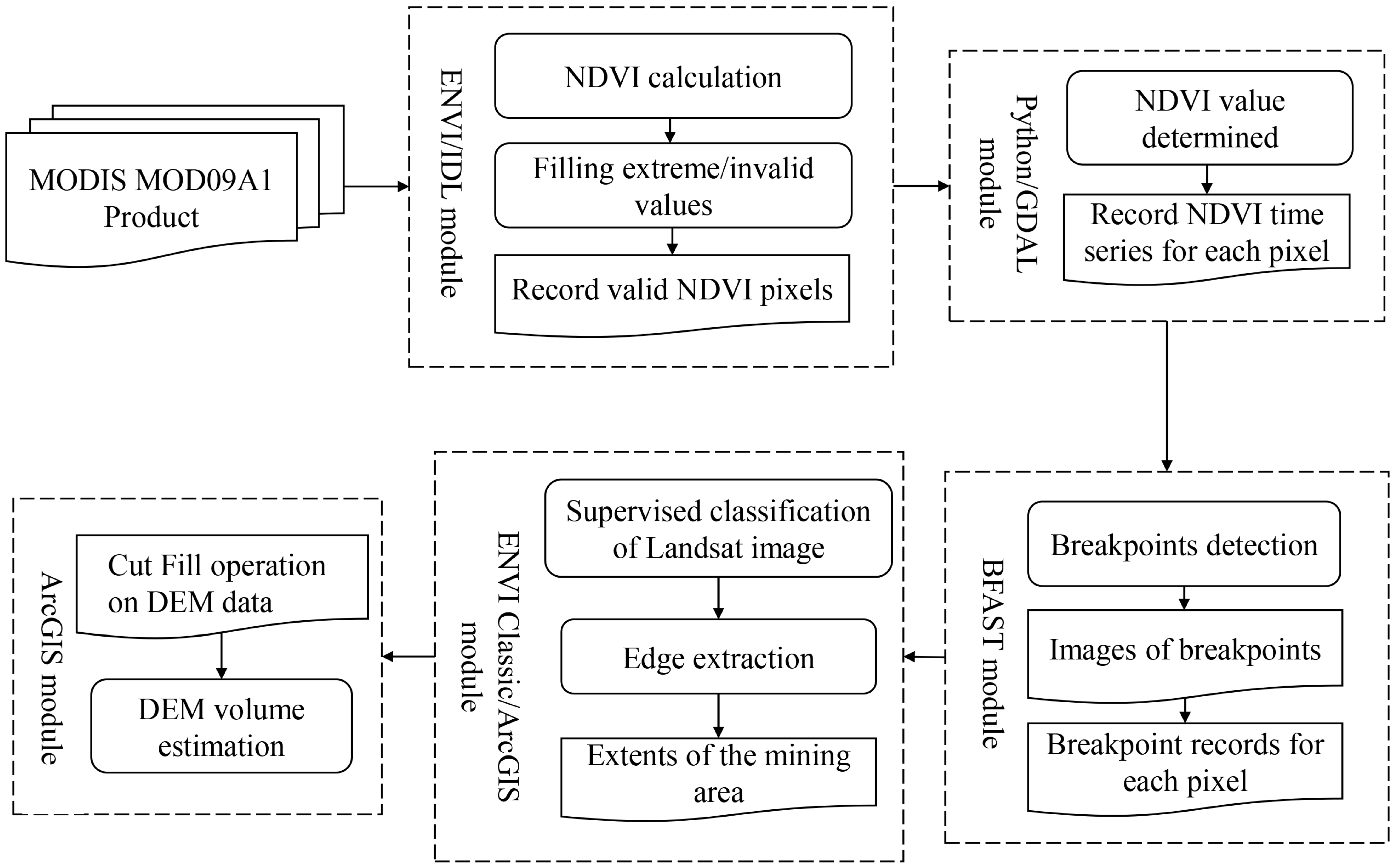
3. Data and Methodology
3.1. Data and Processing
3.2. Methods
3.2.1. Preprocessing of NDVI Time Series
3.2.2. Identification of Mining-Ruined Areas Based on BFAST-Detected NDVI Time Series
- (1)
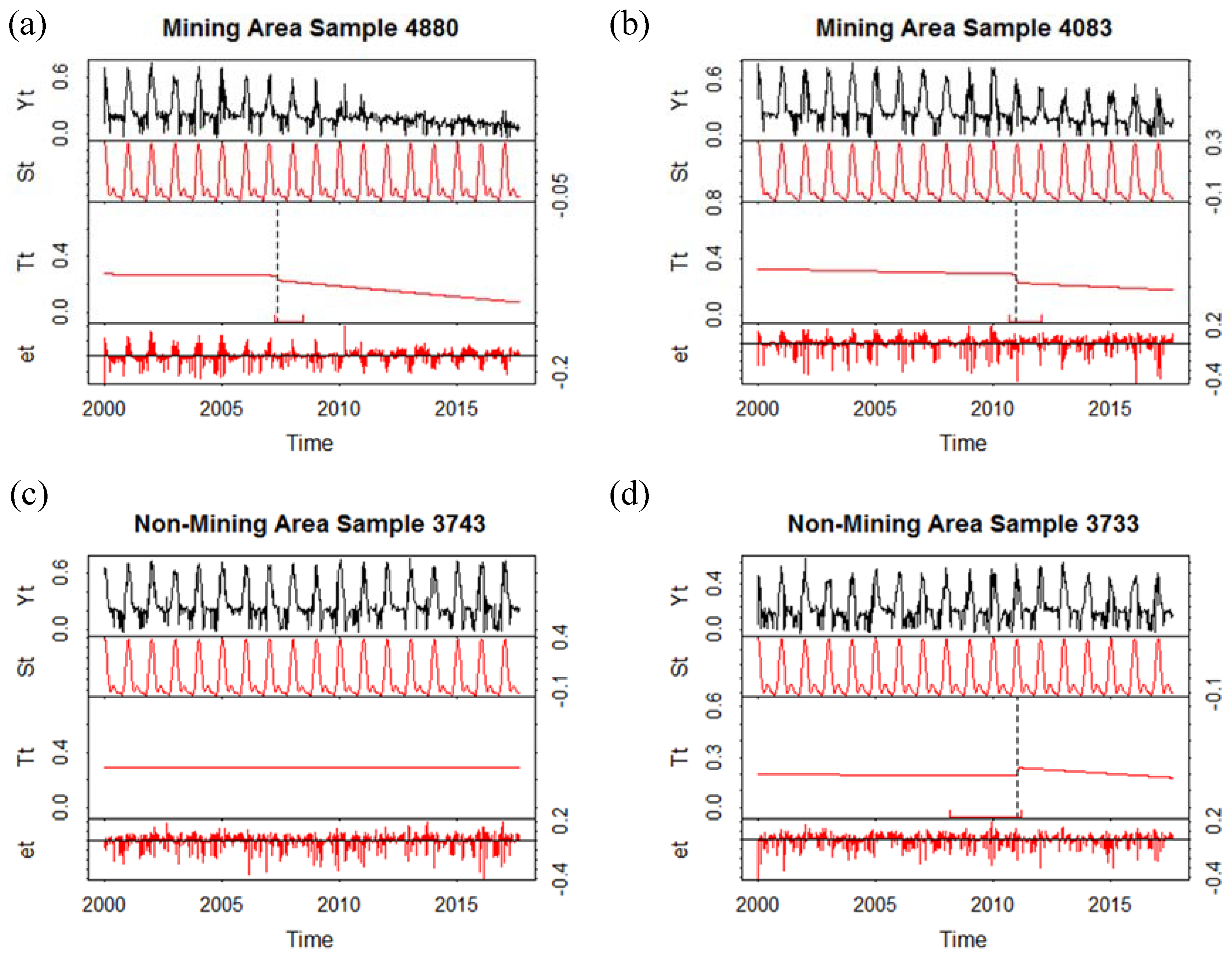
- There is one breakpoint detected in the time series. Assuming that one pixel is located in the new mining area, the NDVI time series of the pixel will show structural decreases after the mining activity. Based on the BFAST algorithm, one breakpoint should be detected if the mining-ruined areas have not yet recovered ecologically.
- (2)
- There is a decrease in NDVI magnitude in the trend components after the breakpoint. As the mining destruction of the land surface is an irreversible process in a short term and the value of NDVI after mining is generally lower than that in the beginning.where represents the last value in the trend component of the first segment, and denotes the first value in the trend component of the second segment.
- (3)
- The magnitude of the post-breakpoint NDVI decrease is larger than the threshold 0.1. We used the difference between the mean NDVI value in the first segment and the mean NDVI value in the last segment to measure the level of NDVI decrease before and after the breakpoints. With a large NDVI decrease, we assume the change is probably associated with coal mining. The optimum threshold value for the change magnitude was set to 0.1 based on our tests on the threshold sensitivity, which will be discussed in the next section.
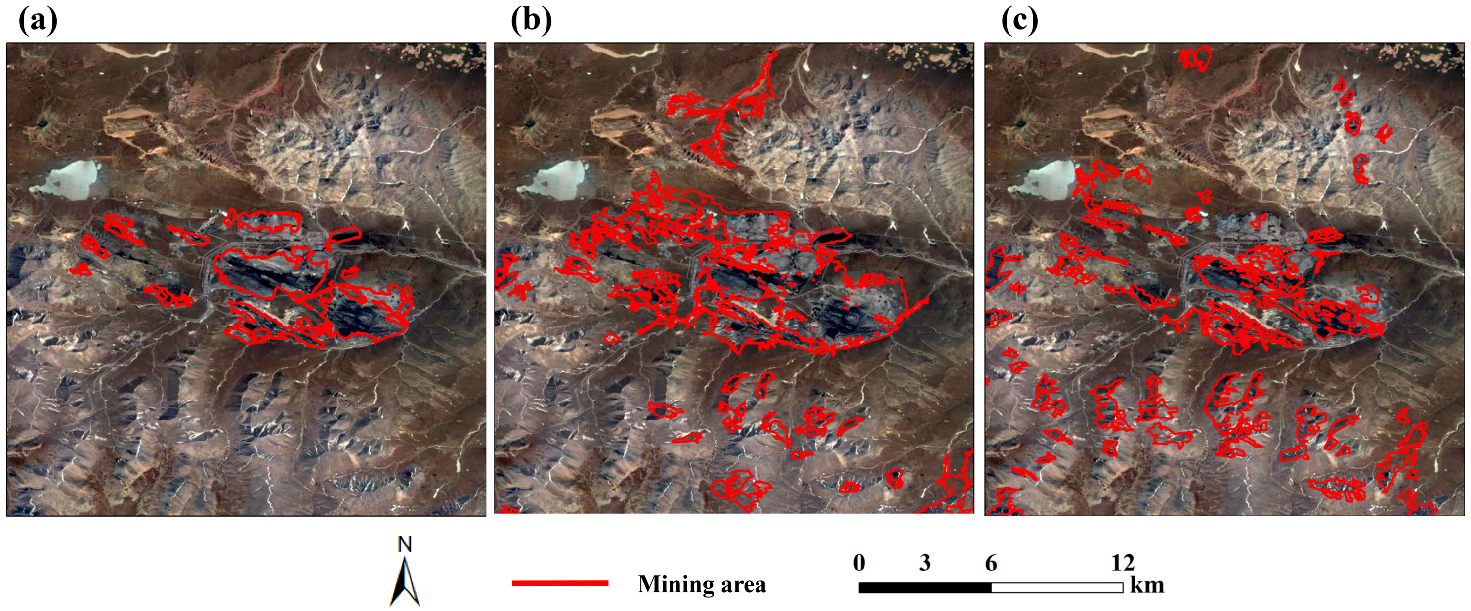
3.2.3. Extraction of Mining Areas from Landsat Imagery
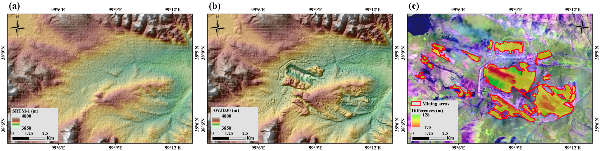
3.2.4. Estimation of Mining Landmass Volume
4. Results and Analyses
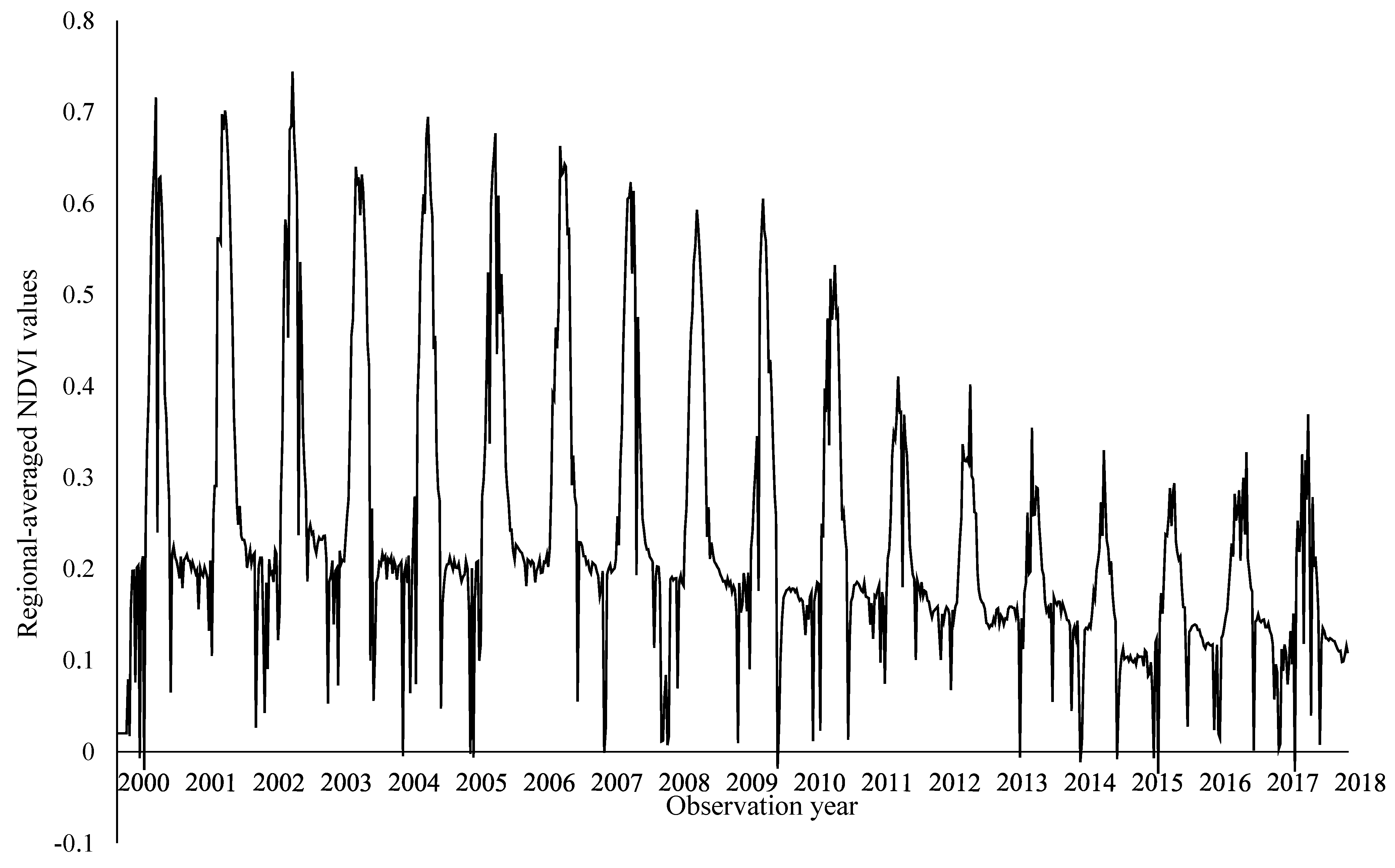
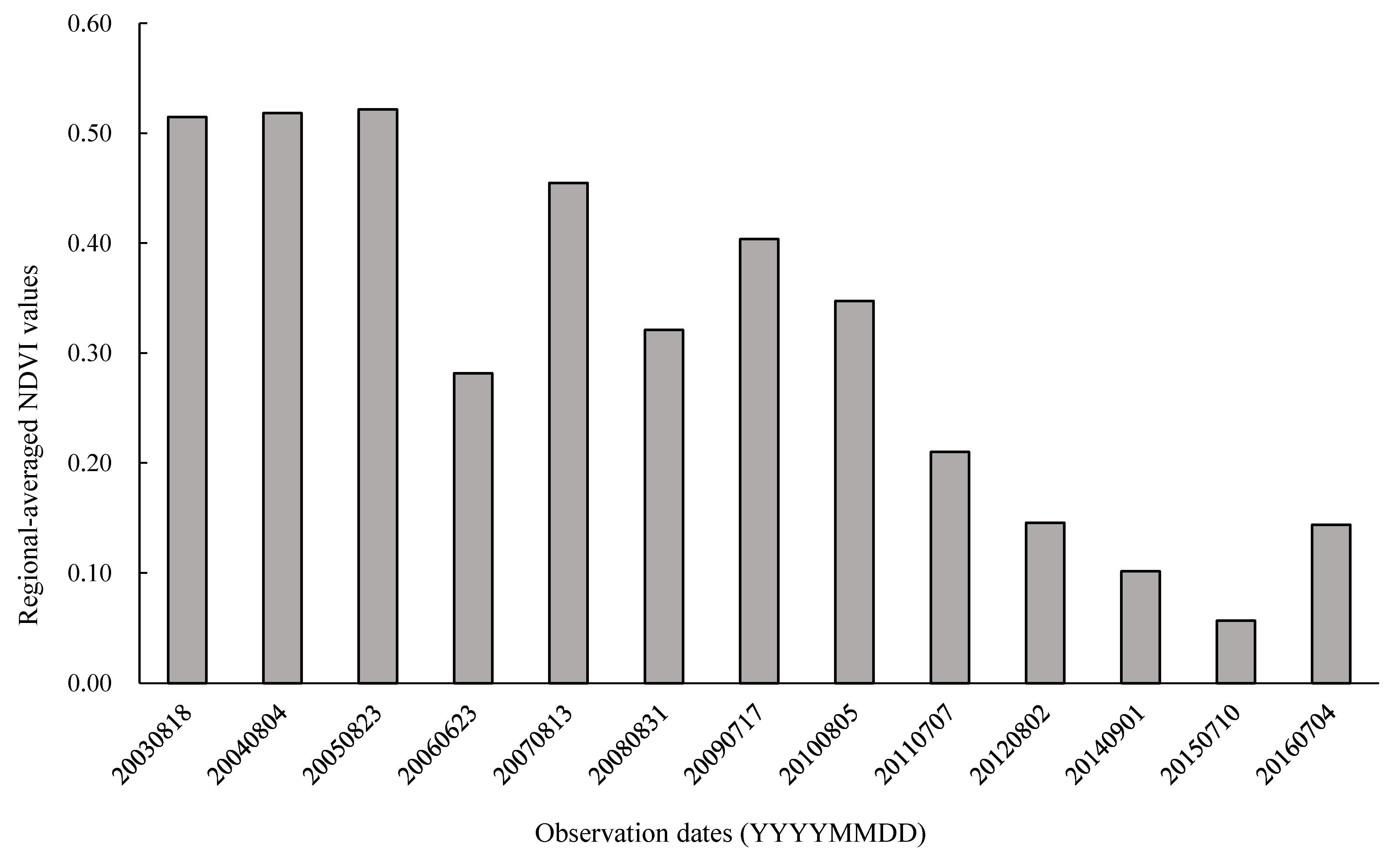
4.1. Abrupt Changes of NDVI Time Series Due to Mining Activities
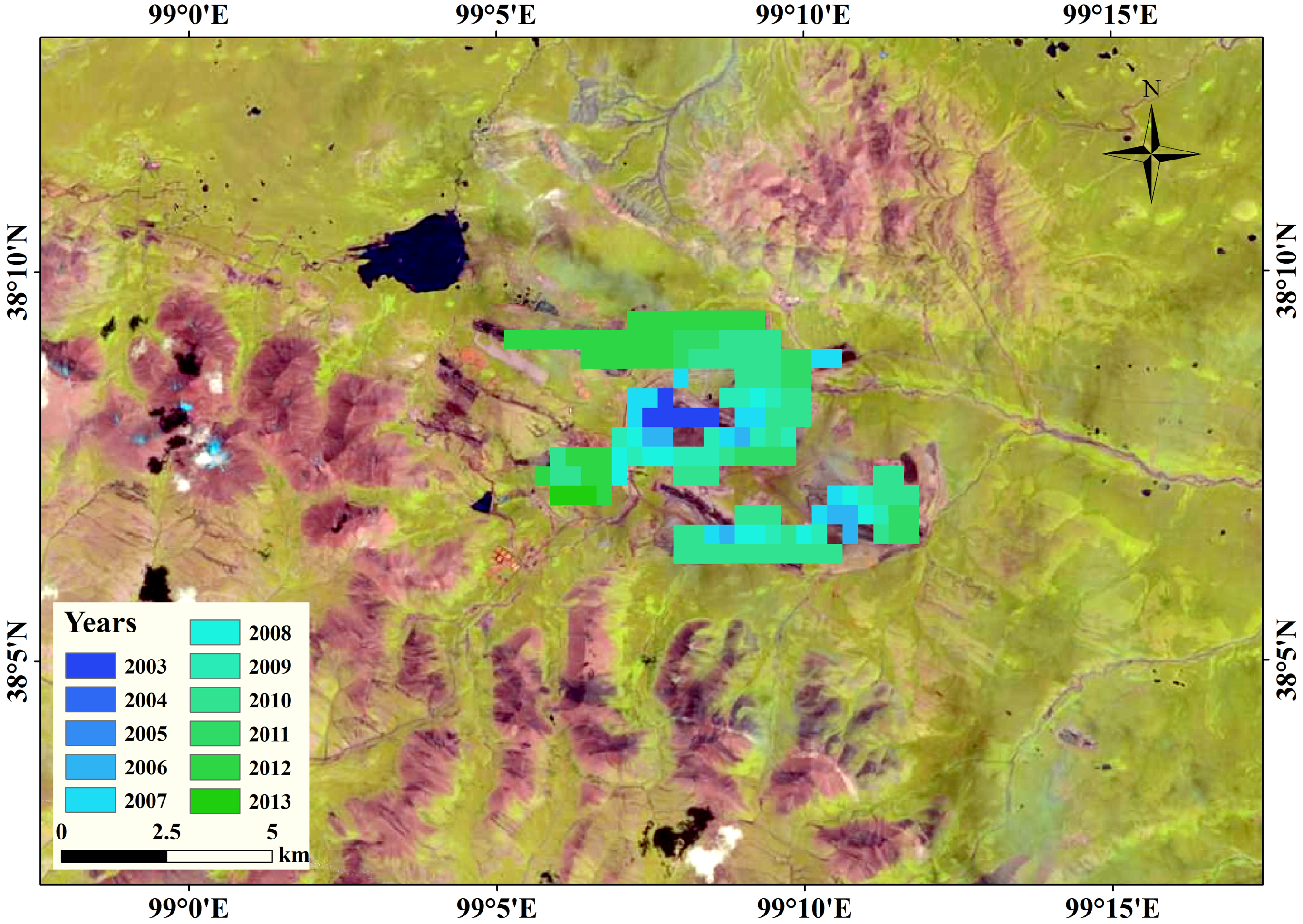
4.2. Mining-Induced Landmass Volume Changes
5. Discussions
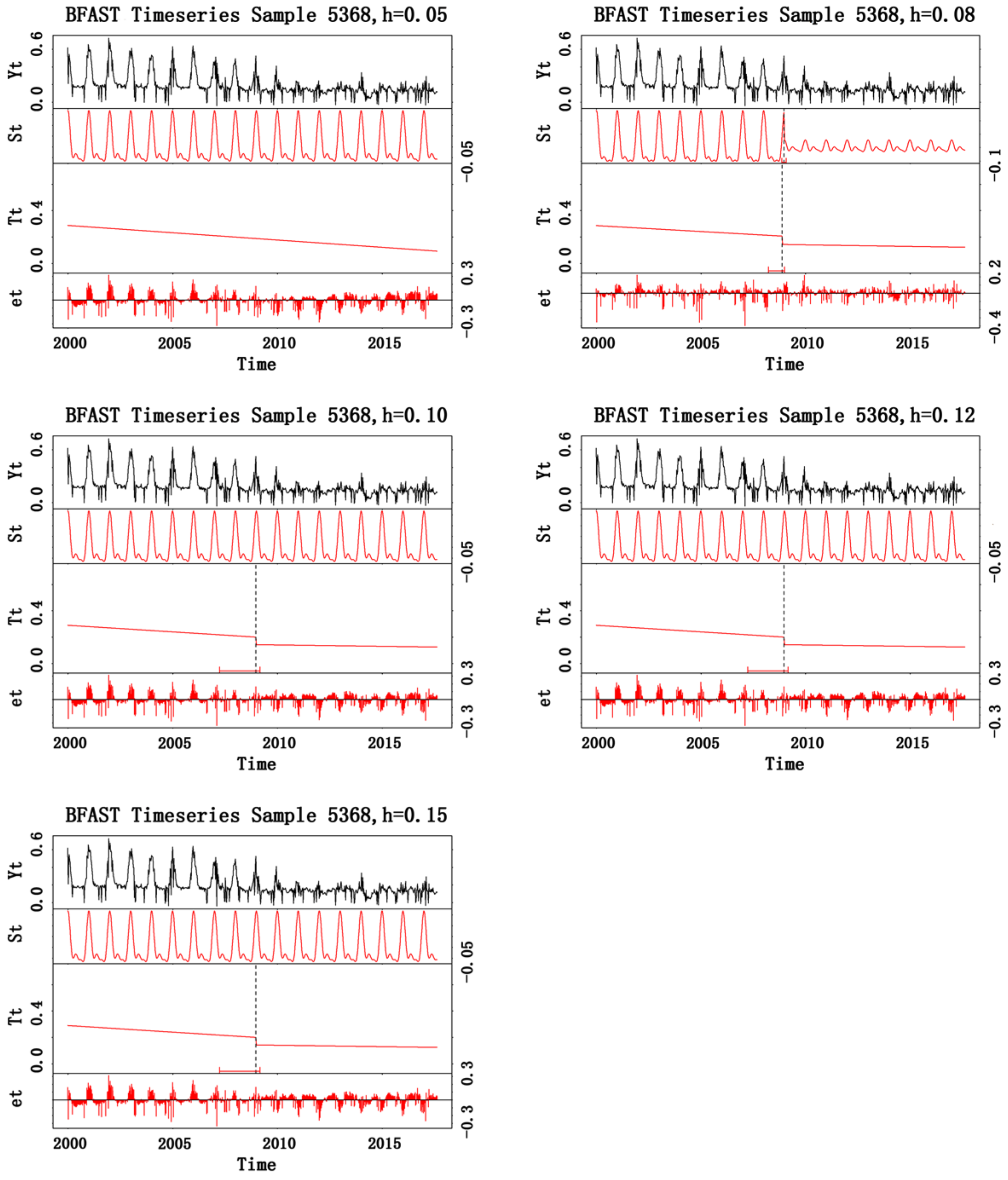
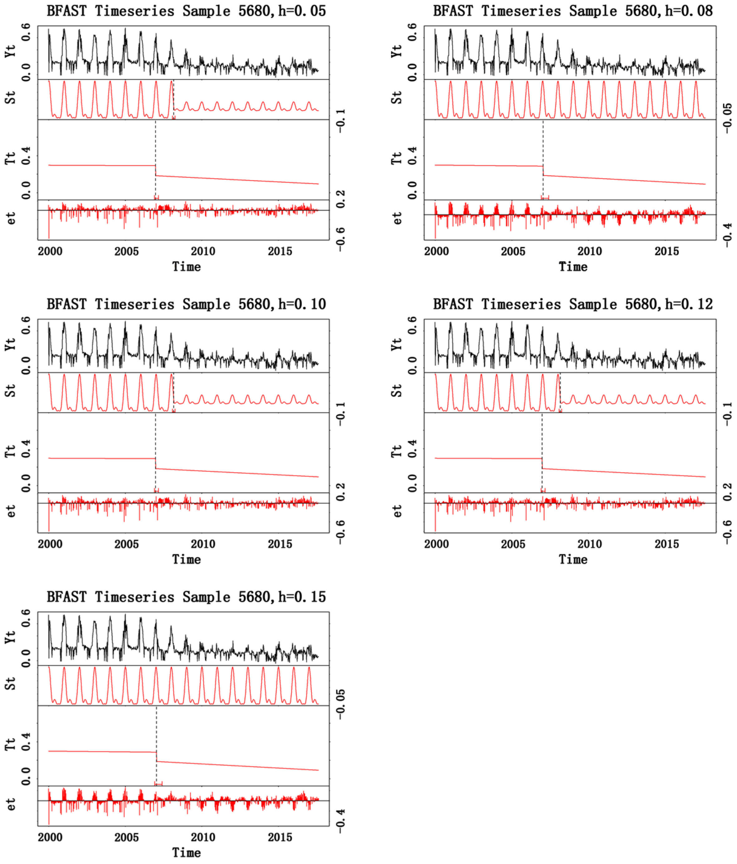
5.1. Sensitivity of BFAST Detection of Abrupt Changes
5.1.1. Sensitivity Test of the h Parameter in BFAST
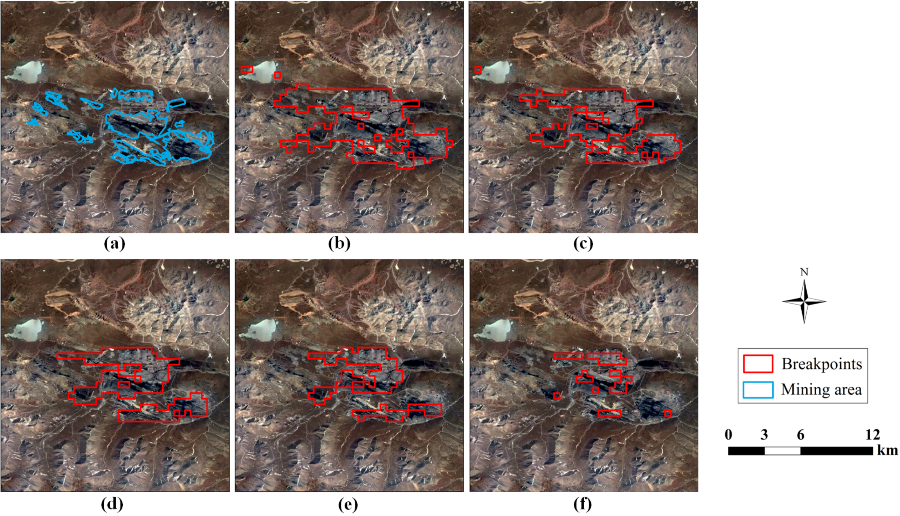
5.1.2. Sensitivity Test of the NDVI Different Threshold
5.2. Influences of Mining Activities on Environmental Damages on the TP
6. Conclusions
Author Contributions
Funding
Acknowledgments
Conflicts of Interest
References
- Yao, T.; Thompson, L.G.; Mosbrugger, V.; Zhang, F.; Ma, Y.; Luo, T.; Xu, B.; Yang, X.; Joswiak, D.R.; Wang, W. Third pole environment (TPE). Environ. Dev. 2012, 3, 52–64. [Google Scholar] [CrossRef]
- Qiu, J. China: The third pole. Nat. News 2008, 454, 393–396. [Google Scholar] [CrossRef] [PubMed] [Green Version]
- Wu, G.; Liu, Y.; Zhang, Q.; Duan, A.; Wang, T.; Wan, R.; Liu, X.; Li, W.; Wang, Z.; Liang, X. The influence of mechanical and thermal forcing by the Tibetan Plateau on Asian climate. J. Hydrometeorol. 2007, 8, 770–789. [Google Scholar] [CrossRef]
- Yang, K.; Wu, H.; Qin, J.; Lin, C.; Tang, W.; Chen, Y. Recent climate changes over the Tibetan Plateau and their impacts on energy and water cycle: A review. Glob. Planet. Chang. 2014, 112, 79–91. [Google Scholar] [CrossRef]
- Zeng, N.; Neelin, J.D.; Lau, K.-M.; Tucker, C.J. Enhancement of interdecadal climate variability in the Sahel by vegetation interaction. Science 1999, 286, 1537–1540. [Google Scholar] [CrossRef] [PubMed]
- Cornelissen, J.H.; Van Bodegom, P.M.; Aerts, R.; Callaghan, T.V.; Van Logtestijn, R.S.; Alatalo, J.; Stuart Chapin, F.; Gerdol, R.; Gudmundsson, J.; Gwynn-Jones, D. Global negative vegetation feedback to climate warming responses of leaf litter decomposition rates in cold biomes. Ecol. Lett. 2007, 10, 619–627. [Google Scholar] [CrossRef] [PubMed]
- Shen, M.; Piao, S.; Jeong, S.-J.; Zhou, L.; Zeng, Z.; Ciais, P.; Chen, D.; Huang, M.; Jin, C.-S.; Li, L.Z. Evaporative cooling over the Tibetan Plateau induced by vegetation growth. Proc. Natl. Acad. Sci. USA 2015, 112, 9299–9304. [Google Scholar] [CrossRef] [PubMed] [Green Version]
- Piao, S.; Cui, M.; Chen, A.; Wang, X.; Ciais, P.; Liu, J.; Tang, Y. Altitude and temperature dependence of change in the spring vegetation green-up date from 1982 to 2006 in the Qinghai-Xizang plateau. Agric. For. Meteorol. 2011, 151, 1599–1608. [Google Scholar] [CrossRef]
- Zhang, G.; Zhang, Y.; Dong, J.; Xiao, X. Green-up dates in the Tibetan Plateau have continuously advanced from 1982 to 2011. Proc. Natl. Acad. Sci. USA 2013, 110, 4309–4314. [Google Scholar] [CrossRef] [PubMed] [Green Version]
- Gao, Y.; Zhou, X.; Wang, Q.; Wang, C.; Zhan, Z.; Chen, L.; Yan, J.; Qu, R. Vegetation net primary productivity and its response to climate change during 2001–2008 in the Tibetan Plateau. Sci. Total. Environ. 2013, 444, 356–362. [Google Scholar] [CrossRef] [PubMed]
- Cheng, G.; Wu, T. Responses of permafrost to climate change and their environmental significance, Qinghai-Tibet Plateau. J. Geophys. Res. Earth Surf. 2007, 112, F02S03. [Google Scholar] [CrossRef]
- Yang, B.; He, M.; Shishov, V.; Tychkov, I.; Vaganov, E.; Rossi, S.; Ljungqvist, F.C.; Bräuning, A.; Grießinger, J. New perspective on spring vegetation phenology and global climate change based on Tibetan Plateau tree-ring data. Proc. Natl. Acad. Sci. USA 2017, 114, 6966–6971. [Google Scholar] [CrossRef] [PubMed] [Green Version]
- Zeng, C.; Wu, J.; Zhang, X. Effects of grazing on above-vs. Below-ground biomass allocation of alpine grasslands on the northern Tibetan Plateau. PLoS ONE 2015, 10, e0135173. [Google Scholar] [CrossRef] [PubMed]
- Kang, S.; Xu, Y.; You, Q.; Flügel, W.-A.; Pepin, N.; Yao, T. Review of climate and cryospheric change in the Tibetan Plateau. Environ. Res. Lett. 2010, 5, 015101. [Google Scholar] [CrossRef] [Green Version]
- Song, C.; Ke, L.; Richards, K.S.; Cui, Y. Homogenization of surface temperature data in high mountain Asia through comparison of reanalysis data and station observations. Int. J. Clim. 2016, 36, 1088–1101. [Google Scholar] [CrossRef]
- You, Q.; Min, J.; Zhang, W.; Pepin, N.; Kang, S. Comparison of multiple datasets with gridded precipitation observations over the Tibetan Plateau. Clim. Dyn. 2015, 45, 791–806. [Google Scholar] [CrossRef] [Green Version]
- Piao, S.; Tan, K.; Nan, H.; Ciais, P.; Fang, J.; Wang, T.; Vuichard, N.; Zhu, B. Impacts of climate and CO2 changes on the vegetation growth and carbon balance of Qinghai-Tibetan grasslands over the past five decades. Glob. Planet. Chang. 2012, 98, 73–80. [Google Scholar] [CrossRef]
- Lin, X.; Zhang, Z.; Wang, S.; Hu, Y.; Xu, G.; Luo, C.; Chang, X.; Duan, J.; Lin, Q.; Xu, B. Response of ecosystem respiration to warming and grazing during the growing seasons in the alpine meadow on the Tibetan Plateau. Agric. For. Meteorol. 2011, 151, 792–802. [Google Scholar] [CrossRef]
- Tan, K.; Ciais, P.; Piao, S.; Wu, X.; Tang, Y.; Vuichard, N.; Liang, S.; Fang, J. Application of the orchidee global vegetation model to evaluate biomass and soil carbon stocks of Qinghai-Tibetan grasslands. Glob. Biogeochem. Cycles 2010, 24. [Google Scholar] [CrossRef]
- Klein, J.A.; Harte, J.; Zhao, X.Q. Experimental warming causes large and rapid species loss, dampened by simulated grazing, on the Tibetan Plateau. Ecol. Lett. 2004, 7, 1170–1179. [Google Scholar] [CrossRef]
- Che, M.; Chen, B.; Innes, J.L.; Wang, G.; Dou, X.; Zhou, T.; Zhang, H.; Yan, J.; Xu, G.; Zhao, H. Spatial and temporal variations in the end date of the vegetation growing season throughout the Qinghai-Tibetan Plateau from 1982 to 2011. Agric. For. Meteorol. 2014, 189, 81–90. [Google Scholar] [CrossRef]
- Shen, M.; Zhang, G.; Cong, N.; Wang, S.; Kong, W.; Piao, S. Increasing altitudinal gradient of spring vegetation phenology during the last decade on the Qinghai-Tibetan Plateau. Agric. For. Meteorol. 2014, 189, 71–80. [Google Scholar] [CrossRef]
- Wu, J.; Zhang, X.; Shen, Z.; Shi, P.; Xu, X.; Li, X. Grazing-exclusion effects on aboveground biomass and water-use efficiency of alpine grasslands on the northern Tibetan Plateau. Rangel. Ecol. Manag. 2013, 66, 454–461. [Google Scholar] [CrossRef]
- An, R.; Wang, H.-L.; Feng, X.-Z.; Wu, H.; Wang, Z.; Wang, Y.; Shen, X.-J.; Lu, C.-H.; Quaye-Ballard, J.A.; Chen, Y.-H. Monitoring rangeland degradation using a novel local NPP scaling based scheme over the “Three-river headwaters” region, hinterland of the Qinghai-Tibetan Plateau. Quat. Int. 2017, 444, 97–114. [Google Scholar] [CrossRef]
- Chen, B.; Zhang, X.; Tao, J.; Wu, J.; Wang, J.; Shi, P.; Zhang, Y.; Yu, C. The impact of climate change and anthropogenic activities on alpine grassland over the Qinghai-Tibet Plateau. Agric. For. Meteorol. 2014, 189, 11–18. [Google Scholar] [CrossRef]
- Wu, J.; Feng, Y.; Zhang, X.; Wurst, S.; Tietjen, B.; Tarolli, P.; Song, C. Grazing exclusion by fencing non-linearly restored the degraded alpine grasslands on the Tibetan Plateau. Sci. Rep. 2017, 7, 15202. [Google Scholar] [CrossRef] [PubMed] [Green Version]
- Harris, R.B. Rangeland degradation on the Qinghai-Tibetan Plateau: A review of the evidence of its magnitude and causes. J. Arid Environ. 2010, 74, 1–12. [Google Scholar] [CrossRef]
- Tucker, C.J.; Pinzon, J.E.; Brown, M.E.; Slayback, D.A.; Pak, E.W.; Mahoney, R.; Vermote, E.F.; El Saleous, N. An extended AVHRR 8-km NDVI dataset compatible with MODIS and spot vegetation NDVI data. Int. J. Remote. Sens. 2005, 26, 4485–4498. [Google Scholar] [CrossRef]
- Watts, L.M.; Laffan, S.W. Effectiveness of the BFAST algorithm for detecting vegetation response patterns in a semi-arid region. Remote. Sens. Environ. 2014, 154, 234–245. [Google Scholar] [CrossRef]
- Tortini, R.; van Manen, S.; Parkes, B.; Carn, S. The impact of persistent volcanic degassing on vegetation: A case study at Turrialba volcano, Costa Rica. Int. J. Appl. Earth Obs. Geoinfor. 2017, 59, 92–103. [Google Scholar] [CrossRef]
- Verbesselt, J.; Hyndman, R.; Newnham, G.; Culvenor, D. Detecting trend and seasonal changes in satellite image time series. Remote. Sens. Environ. 2010, 114, 106–115. [Google Scholar] [CrossRef]
- Angert, A.; Biraud, S.; Bonfils, C.; Henning, C.; Buermann, W.; Pinzon, J.; Tucker, C.; Fung, I. Drier summers cancel out the CO2 uptake enhancement induced by warmer springs. Proc. Natl. Acad. Sci. USA 2005, 102, 10823–10827. [Google Scholar] [CrossRef] [PubMed]
- Scheffer, M.; Carpenter, S.; Foley, J.A.; Folke, C.; Walker, B. Catastrophic shifts in ecosystems. Nature 2001, 413, 591–596. [Google Scholar] [CrossRef] [PubMed]
- Zhao, M.; Running, S.W. Drought-induced reduction in global terrestrial net primary production from 2000 through 2009. Science 2010, 329, 940–943. [Google Scholar] [CrossRef] [PubMed]
- Verbesselt, J.; Hyndman, R.; Zeileis, A.; Culvenor, D. Phenological change detection while accounting for abrupt and gradual trends in satellite image time series. Remote. Sens. Environ. 2010, 114, 2970–2980. [Google Scholar] [CrossRef] [Green Version]
- Fang, H.; Xu, M.; Lin, Z.; Zhong, Q.; Bai, D.; Liu, J.; Pei, F.; He, M. Geophysical characteristics of gas hydrate in the Muli area, Qinghai province. J. Nat. Gas Sci. Eng. 2017, 37, 539–550. [Google Scholar] [CrossRef]
- Wang, T. Gas hydrate resource potential and its exploration and development prospect of the Muli coalfield in the northeast Tibetan Plateau. Energy Explor. Exploit. 2010, 28, 147–157. [Google Scholar] [CrossRef]
- Zhang, Q.-B.; Qiu, H. A millennium-long tree-ring chronology of sabina przewalskii on northeastern Qinghai-Tibetan Plateau. Dendrochronologia 2007, 24, 91–95. [Google Scholar] [CrossRef]
- Han, W.; Fang, J.; Guo, D.; Zhang, Y. Leaf nitrogen and phosphorus stoichiometry across 753 terrestrial plant species in China. New Phytol. 2005, 168, 377–385. [Google Scholar] [CrossRef] [PubMed] [Green Version]
- Wang, C.T.; Long, R.J.; Wang, Q.J.; Ding, L.M.; Wang, M.P. Effects of altitude on plant-species diversity and productivity in an alpine meadow, Qinghai-Tibetan Plateau. Aust. J. Bot. 2007, 55, 110–117. [Google Scholar] [CrossRef]
- Lunetta, R.S.; Knight, J.F.; Ediriwickrema, J.; Lyon, J.G.; Worthy, L.D. Land-cover change detection using multi-temporal MODIS NDVI data. Remote. Sens. Environ. 2006, 105, 142–154. [Google Scholar] [CrossRef]
- Beck, P.S.; Atzberger, C.; Høgda, K.A.; Johansen, B.; Skidmore, A.K. Improved monitoring of vegetation dynamics at very high latitudes: A new method using MODIS NDVI. Remote. Sens. Environ. 2006, 100, 321–334. [Google Scholar] [CrossRef]
- Vermote, E. MOD09A1 MODIS/Terra surface reflectance 8-day l3 global 500 m sin grid v006. NASA Eosdis Land Process. DAAC 2015, 10. [Google Scholar] [CrossRef]
- Tadono, T.; Takaku, J.; Tsutsui, K.; Oda, F.; Nagai, H. Status of ALOS World 3D (AW3D) Global DSM Generation. In Proceedings of the IEEE International Geoscience and Remote Sensing Symposium (IGARSS), Milan, Italy, 26–31 July 2015; pp. 3822–3825. [Google Scholar]
- Peng, J.; Liu, Z.; Liu, Y.; Wu, J.; Han, Y. Trend analysis of vegetation dynamics in Qinghai-Tibet Plateau using Hurst exponent. Ecol. Indic. 2012, 14, 28–39. [Google Scholar] [CrossRef]
- Shen, X.; An, R.; Feng, L.; Ye, N.; Zhu, L.; Li, M. Vegetation changes in the Three-river headwaters region of the Tibetan Plateau of China. Ecol. Indic. 2018, 93, 804–812. [Google Scholar] [CrossRef]
- Immerzeel, W.W.; Van Beek, L.P.; Bierkens, M.F. Climate change will affect the Asian water towers. Science 2010, 328, 1382–1385. [Google Scholar] [CrossRef] [PubMed]
- Huang, X.; Sillanpää, M.; Duo, B.; Gjessing, E.T. Water quality in the Tibetan Plateau: Metal contents of four selected rivers. Environ. Pollut. 2008, 156, 270–277. [Google Scholar] [CrossRef] [PubMed]
- Balerna, A.; Bernieri, E.; Pecci, M.; Polesello, S.; Smiraglia, C.; Valsecchi, S. Chemical and radio-chemical composition of freshsnow samples from northern slopes of Himalayas (cho oyu range, Tibet). Atmos. Environ. 2003, 37, 1573–1581. [Google Scholar] [CrossRef]
- Xiao, C.; Qin, D.; Yao, T.; Ren, J.; Li, Y. Spread of lead pollution over remote regions and upper troposphere: Glaciochemical evidence from polar regions and Tibetan Plateau. Bull. Environ. Contam. Toxicol. 2001, 66, 691–698. [Google Scholar] [CrossRef] [PubMed]
- Zhou, Y.; Guo, D.; Qiu, G.; Cheng, G.; Li, S. Permafrost in China; Science: Beijing, China, 2000; pp. 403–404. [Google Scholar]
- Cao, W.; Sheng, Y.; Qi, J.-L. Assessment of the permafrost environment in the Muli mining area in Qinghai province based on catastrophe progression method. J. China Coal Soc. 2008, 33, 881–886. [Google Scholar]
- Wang, G.; Yao, J.; Guo, Z.; Wu, Q.; Wang, Y. Human engineering activities on frozen soil ecosystem change and its effect on railway construction. Chin. Sci. Bull. 2004, 49, 1556–1564. [Google Scholar] [CrossRef]


| h | Trend Breakpoints | Seasonal Breakpoints | ||||
|---|---|---|---|---|---|---|
| Corresponding to Breakdates: | Corresponding to Breakdates: | |||||
| 2.5% | Breakpoints | 97.5% | 2.5% | Breakpoints | 97.5% | |
| 0.05 | None | None | ||||
| 0.08 | 29 Marth 2008 | 24 November 2008 | 1 January 2009 | 16 November 2008 | 26 December 2008 | 02 February 2009 |
| 0.10 | 30 Marth 2007 | 26 December 2008 | 06 Marth 2009 | None | ||
| 0.12 | 30 Marth 2007 | 26 December 2008 | 06 Marth 2009 | None | ||
| 0.15 | 30 Marth 2007 | 26 December 2008 | 06 Marth 2009 | None | ||
| h | Trend Breakpoints | Seasonal Breakpoints | ||||
|---|---|---|---|---|---|---|
| Corresponding to Breakdates: | Corresponding to Breakdates: | |||||
| 2.5% | Breakpoints | 97.5% | 2.5% | Breakpoints | 97.5% | |
| 0.05 | 3 December 2006 | 27 December 2006 | 6 Marth 2007 | 2 February 2008 | 5 March 2008 | 6 April 2008 |
| 0.08 | 11 December 2006 | 17 January 2007 | 2 June 2007 | None | ||
| 0.10 | 3 December 2006 | 27 December 2006 | 06 Marth 2007 | 2 February 2008 | 5 March 2008 | 6 April 2008 |
| 0.12 | 3 December 2006 | 27 December 2006 | 06 Marth 2007 | 2 February 2008 | 5 March 2008 | 6 April 2008 |
| 0.15 | 11 December 2006 | 17 January 2007 | 2 June 2007 | None | ||
| Threshold | 0.05 | 0.08 | 0.10 | 0.12 | 0.15 |
|---|---|---|---|---|---|
| Overall accuracy | 0.9670 | 0.9736 | 0.9760 | 0.9783 | 0.9779 |
| Kappa index | 0.5320 | 0.5560 | 0.5552 | 0.5029 | 0.2741 |
© 2018 by the authors. Licensee MDPI, Basel, Switzerland. This article is an open access article distributed under the terms and conditions of the Creative Commons Attribution (CC BY) license (http://creativecommons.org/licenses/by/4.0/).
Share and Cite
Wu, Q.; Liu, K.; Song, C.; Wang, J.; Ke, L.; Ma, R.; Zhang, W.; Pan, H.; Deng, X. Remote Sensing Detection of Vegetation and Landform Damages by Coal Mining on the Tibetan Plateau. Sustainability 2018, 10, 3851. https://0-doi-org.brum.beds.ac.uk/10.3390/su10113851
Wu Q, Liu K, Song C, Wang J, Ke L, Ma R, Zhang W, Pan H, Deng X. Remote Sensing Detection of Vegetation and Landform Damages by Coal Mining on the Tibetan Plateau. Sustainability. 2018; 10(11):3851. https://0-doi-org.brum.beds.ac.uk/10.3390/su10113851
Chicago/Turabian StyleWu, Qianhan, Kai Liu, Chunqiao Song, Jida Wang, Linghong Ke, Ronghua Ma, Wensong Zhang, Hang Pan, and Xinyuan Deng. 2018. "Remote Sensing Detection of Vegetation and Landform Damages by Coal Mining on the Tibetan Plateau" Sustainability 10, no. 11: 3851. https://0-doi-org.brum.beds.ac.uk/10.3390/su10113851