Berth Scheduling Problem Considering Traffic Limitations in the Navigation Channel

Abstract

In view of the trend of upsizing ships, the physical limitations of natural waterways, huge expenses, and unsustainable environmental impact of channel widening, this paper aims to provide a cost-efficient but applicable solution to improve the operational performance of container terminals that are enduring inefficiency caused by channel traffic limitations. We propose a novel berth scheduling problem considering the traffic limitations in the navigation channel, which appears in many cases including insufficient channel width, bad weather, poor visibility, channel accidents, maintenance dredging of the navigation channel, large vessels passing through the channel, and so on. To optimally utilize the berth and improve the service quality for customers, we propose a mixed-integer linear programming model to formulate the berth scheduling problem under the one-way ship traffic rule in the navigation channel. Furthermore, we develop a more generalized model which can cope with hybrid traffic in the navigation channel including one-way traffic, two-way traffic, and temporary closure of the navigation channel. For large-scale problems, a hybrid simulated annealing algorithm, which employs a problem-specific heuristic, is presented to reduce the computational time. Computational experiments are performed to evaluate the effectiveness and practicability of the proposed method.

1. Introduction

Maritime transportation has a major role in driving economic growth and globalization, as it accounts for four fifths of the world’s total merchandise trade [1]. It has been well documented that any operational inefficiency in container ports may cause a bottleneck in the global supply chain that damages to the efficiency and sustainability of international trade, especially that of the globalized manufacturing industry [2,3,4]. The optimal allocation of port resources is an important guarantee for the sustainable development of marine transportation industry [5].

In many container ports worldwide, including some of the top ranked ports in terms of throughput, vessels entering and leaving have to pass through navigation channels, which significantly limits the operational efficiency of container terminals. In recent years, vessels calling at terminals have dramatically increased in size and capacity attaining up to 21000 TEUs and larger sizes are being planned. The authorities of ports have been forced to invest heavily to accommodate these vessels by widening and deepening navigation channels. However, such channel improvements are costly and time-consuming, and always lag behind the continuous enlargement of vessel size. More importantly, the channel widening is not sustainable due to its environmental impacts and the physical limitations of natural waterways. For example, additional dredging needed in the channel widening has some persistent environmental effects, including damage to shallow-water estuarine ecosystems and take of imperiled species [6].

For the sake of navigation safety, traffic limitations in the navigation channels, such as the one way navigation rule and temporary closure of navigation channels, are commonly adopted in many cases including insufficient channel width, bad weather, poor visibility, channel accidents, maintenance dredging of the navigation channel [7], large vessels passing through the channel, and so on. For example, in the Port of Tianjin, one of the top 10 largest ports in the world both in terms of throughput and TEU handled [8], only one-way ship traffic is allowed in the navigation channel when there are strong winds, and if the wind speed reaches 20.8 m/s, no ship traffic is allowed in the navigation channel [9]. In one-way traffic periods, ship traffic can only move in one direction in the channel, alternating every 4 hours between outward traffic and inward traffic. In the Port of Guangzhou, the largest port in South China, one-way traffic is enforced when ships of more than 50,000 DWT pass through the channel from the Nansha port area to the Pearl River estuary [10]. There are also some ports, such as the Port of Tanjung Priok, the busiest and most advanced Indonesian seaport, whose navigation channel can only support one-way traffic due to the physical limitations of the natural waterway [11].

In practice, the efficiency of terminal operation is severely restricted by the traffic limitations of the navigation channel. For example, vessels calling at the port may have to wait a long time at the outer anchorage until the navigation channel becomes available for entering/inward traffic, even when the berth is available. Likewise, vessels having finished handling at the berth and ready for leaving may also have to wait a long time for the navigation channel to become available for leaving/outward traffic. Accordingly, the complexity of the berth scheduling problem in terminals is significantly increased and hard to cope with by approaches used in conventional berth scheduling studies. However, due to the trend of upsizing ships, the huge expense and environmental impact of channel widening and the physical limitations of natural waterways, more and more terminal operators will have to face this problem. The unnecessary waiting times of ships causes a negative economic and environmental impact related to fuel consumption and route timing [12]. In particular, the waiting time of the ships has an important influence on the volume emissions, where having flowing operations can help shipping companies to reduce emissions as well as help ports to have control over that [13].

Motivated by the aforementioned facts, this paper aims to provide a cost-efficient but applicable solution to improve the operational performance of container terminals that are enduring inefficiency caused by channel traffic limitations. To achieve this, we investigate a novel berth scheduling problem considering traffic limitations in the navigation channel (referred to as BSPCTW below). To better utilize the berth and improve the service quality for customers, we develop a mixed-integer linear programming model to optimize the berth scheduling under one-way ship traffic rule in the navigation channel. Then, we propose a more generalized model that can cope with hybrid traffic in the navigation channel including one-way traffic, two-way traffic and temporary closure of the navigation channel. Furthermore, we present an efficient hybrid meta-heuristic algorithm that can significantly reduce the solving time of the proposed model relative to CPLEX when the workload of berth is heavy.

The remainder of this paper is organized as follows. In Section 2, we review the literature related to this study. In Section 3, we describe the proposed problem, and present the basic model and the generalized model for the berth scheduling problem considering the traffic limitations in the navigation channel. Section 4 describes the hybrid meta-heuristic method that is used to solve the proposed problem. Section 5 presents the computational experiments and results. Finally, Section 6 draws the conclusions for this research.

2. Literature Review

To enhance the competitiveness of container terminals, terminal managers always attempt to maximize the efficiency of terminal operations by improving the utilization of terminal facilities. In this context, an ever increasing number of studies on modeling and optimization of terminal operations have appeared in the literature over the past two decades, including studies on berth scheduling [14], yard space allocation [15], crane scheduling [16], container stacking [17] and so on. Among all these problems, berth scheduling problem (BSP), which aims to optimally assign berthing times and positions to vessels, lies in the kernel position, because the berth plan is the basis for making almost all the other operation plans in container terminals, and it has a great influence on yard space allocation, quay/yard crane scheduling and even container stacking.

According to the classification proposed by Bierwirth and Meisel [14], a multitude of variants for the BSP have been studied. In general, the following classification schemes can be applied: (a) static versus dynamic vessel arrivals, (b) discrete versus continuous berthing space. In a static BSP, all of the vessels have already arrived at the port at the beginning of the planning horizon [18,19], whereas in a dynamic BSP, vessels can arrive at any moment of the planning horizon [20,21]. In the BSP with discrete berthing space (namely BSPD) studies, the quay is divided into a finite set of fixed-length berths (namely discrete berths) and each berth can only serve one vessel at a time, while in the BSP with continuous berthing space (namely BSPC) studies vessels are allowed to berth anywhere along the quay. In addition, BSP with hybrid berth space has also been studied [22], where the quay is partitioned into berths, but vessels may share a berth or one vessel may occupy more than one berth. A particular form of a hybrid berth is an indented berth where large vessels can be served from two oppositely located berths [23].

Obviously, relative to BSPD, BSPC provides more flexibility for berth scheduling and utilizes the quay space more effectively, but it also significantly increases the complexity of the problem, which makes the solving process much more difficult. To make full use of berth in container terminals, our research on the BSPCTW proposed in this paper is based on BSPC. Lim [24] first addressed BAPC and formulated the BAPC as a two-dimensional packing problem. Li et al. [19] consider the BSPC as a scheduling problem with a single processor through which multiple jobs can be processed simultaneously. Their model assumes that all vessels have arrived at the terminal before the berthing planning starts. They suggest a heuristic method to determine both the berthing times and the positions of vessels to minimize the makespan. Kim and Moon [25], Guan and Cheung [26] and Wang and Lim [27] consider a more general case of BSPC in which vessels are allowed to arrive at the terminal dynamically after the berthing planning starts. Several solution methods have been proposed for this problem, including a simulated annealing approach [25], a stochastic beam search algorithm [27] and a tree search procedure [26]. For a more comprehensive and detailed review of recent research on the BSPC, we refer the readers to Bierwirth and Meisel [23].

Some recent studies have focused on BSP in emergency or uncertain situations. Hendriks et al. [28], Xu et al. [29], Golias et al. [30], Zhen [31], and Shang et al. [32] focus on robust berth scheduling methods to mitigate the impact of uncertain delay of vessel arrivals and fluctuation of handling time. Xu et al. [33] investigate the collaborative emergency berth scheduling in the situation of unexpected shutdown of a terminal. Another strong research trend on BSP looks at collaboration between terminals [34,35,36] and between terminals and liner shipping companies [37,38,39,40,41].

The above-mentioned studies assume that vessels can enter the port at any time after their arrival and can leave the port at any time after they finish loading and unloading. However, as mentioned in Section 1, such an assumption is impractical in many cases.

Cordeau et al. [42] formulate BSPD considering the service time windows of ships and the availability time windows of berths. They assume that each vessel has a maximal allowable completion time and each berth has an earliest available time and a latest available time. Barros et al. [43], Xu et al. [44], Lalla-Ruiz et al. [45] and Du et al. [4] investigate the berth scheduling problem in tidal ports where the available depth at low tide is inadequate for sailing or berthing of vessels; this shares some similarities with our study. Barros et al. [43] consider a BSPD in tidal bulk ports. By assuming that high tide happens in 12-hour intervals and dividing the planning horizon into several tidal time windows (TTW) of equal length, they convert the problem into one of assigning each ship to a subset of TTW whose length corresponds to the handling time necessary for operation completion. Xu et al. [44] study a BSPD that considers the different water depths of berths (i.e., BAPTL), where the availability of berths is constrained by tide level. By dividing the time horizon into two periods (i.e., low tide period and high tide period), they formulate the problem as mixed integer linear programming models. Lalla-Ruiz et al. [45] propose an alternative mathematical formulation for BAPTL introduced by Xu et al. [44] based upon the generalized set partitioning problem, which allows to tackle the problem with the planning horizon of more than two periods and includes constraints related to berth and vessel time windows. Du et al. [4] factor the consideration of tides into BSPC and retrofit the model of BSPC as a nonlinear programming model. Model transformation tricks based on second-order cone programming are employed to treat the nonlinear intractability in the model.

The study presented in this paper differs from those of Cordeau et al. [42], Barros et al. [43], Xu et al. [44], Lalla-Ruiz et al. [45] and Du et al. [4] in several aspects: (1) The impact of shipping channel traffic restrictions such as one-way navigation restriction, temporary closure of channel and hybrid traffic restrictions, which are commonly imposed in many situations (as mentioned in Section 1), are incorporated in berth scheduling in this paper, whereas such problems are hard to cope with using the approaches presented in Cordeau et al. [42], Barros et al. [43], Xu et al. [44], Lalla-Ruiz et al. [45] and Du et al. [4]. (2) The models of Cordeau et al. [42], Barros et al. [43], Xu et al. [44] and Lalla-Ruiz et al. [45] are based on BSPD, whereas this study is based on BSPC, which can make better use of berth but is more complex and challenging in modeling and solving. (3) Different from Cordeau et al. [42], Xu et al. [44] and Lalla-Ruiz et al. [45], this study focuses on BSP that considers the availability of the navigation channel, rather than the availability of berths. (4) The decision of where berthing is not considered in the study of Barros et al. [43], which is essentially different from our study.

In addition, our research is also related to the study of the waterway ship scheduling problem. Lalla-Ruiz et al. [12] propose the waterway ship scheduling problem (WSSP) in order to schedule incoming and outgoing ships through different waterways for accessing or leaving the port. They formulate the problem as a MILP model. The objective is to minimize the total time required for the ships to pass through the waterways, which contributes to reduce vessel emissions while they are waiting at the anchorage either for entering or leaving. Hill et al. [46] propose a reformulation of the WSSP as a variant of the multi-mode resource-constrained project scheduling problem, which incorporates time-dependent resource capacities besides earliest and latest start times for the tasks.

The main contributions of this paper relative to the existing literature are summarized as follows:

• We are among the first to discuss the continuous berth scheduling problem (BSPC) that considers traffic limitations in the navigation channel such as the one-way navigation rule, temporary closure of the channel, and hybrid restrictions, which are commonly adopted in many situations in container ports (as mentioned in the third paragraph of Section 1).
• We develop a mixed-integer linear programming model that can formulate and resolve the continuous berth scheduling problem under the one-way ship traffic rule in the navigation channel, and further provide a more generalized model that copes well with hybrid traffic in the navigation channel, including one-way traffic, two-way traffic, and temporary closure of channel. Neither problem has been addressed or formulated in previous berth scheduling studies.
• By better scheduling the berth rather than simply widening the channel, which is unsustainable and costly, we provide a new perspective and solution to improve the performance of container terminals that are enduring inefficiency caused by channel traffic limitations.
• We provide an effective and efficient problem-specific algorithm to solve the proposed problems, which can significantly reduce the solving times relative to CPLEX when the workload of the berth is heavy.

3. Problem Formulation

This section presents mathematical models for two cases of the proposed problem. The first one is the model of continuous berth scheduling under one-way traffic restriction in the channel (referred to as the Basic Model below), and the second one is the continuous berth scheduling model that can cope with hybrid traffic restrictions in the channel (referred to as the Generalized Model).

3.1. Berth Scheduling Model under the One-way Traffic Rule in the Channel

One-way traffic restriction is the most commonly adopted measure to ensure the safety of navigation when the navigable channel in the port is of insufficient width, as exemplified in the case of the Port of Tanjung Priok in Section 1. In such cases, ship traffic in the channel is only available in one direction, and the direction alternates at regular intervals between outward traffic and inward traffic. During periods of outward traffic, vessels arriving at the port have to wait at the outer anchorage until the channel becomes available for inward traffic, even when the berth is available. Similarly, vessels that have finished handling cannot leave the berth immediately during periods of inward traffic.

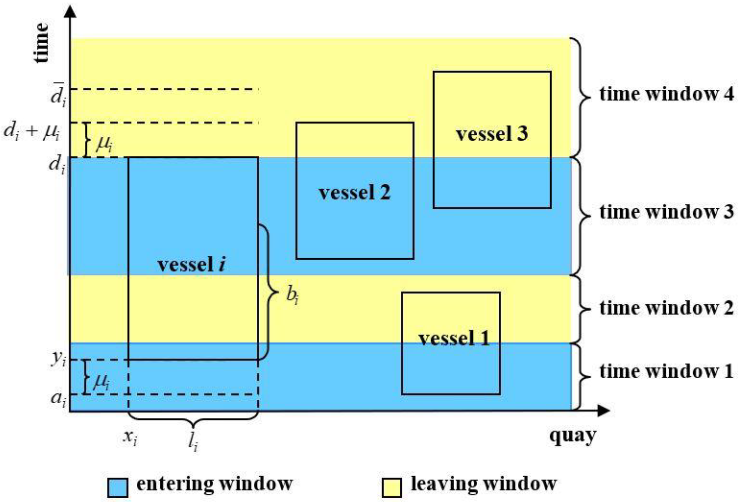
The impacts of one-way traffic restriction on berth scheduling are illustrated in Figure 1, where the horizontal axis represents the position along the quay, and the vertical one is the time axis. The time axis is divided into several intervals that define the time windows for inward traffic and outward traffic in the channel (referred to as the entering window and leaving window respectively). For clarity, we use different colors to represent different types of time windows in the diagram, where the blue zones represent the entering windows and the yellow zones represent the leaving windows. Each rectangle represents a vessel to be served. The width of a rectangle denotes the vessel length, while the height denotes the berth occupancy time, namely, the time length that the corresponding vessel stays at the berth. The horizontal position of the rectangle corresponds to the berthing position of the vessel along the quay. The vertical position of the top edge of the rectangle indicates the departure time of the corresponding vessel and that of the bottom edge indicates the berthing start time.

Different from conventional BSP, the berth occupancy times of vessels (i.e., the heights of rectangles in the quay-time diagram) are variables that are necessarily equal to the handling times of the corresponding vessels. The berthing start times and the departure times of vessels (i.e., the vertical positions of the top edges and bottom edges of rectangles) must be carefully determined to make sure the time intervals of vessels passing through the channel lie in time windows of the right type. These distinctive features make it more challenging to balance the service qualities of different vessels and optimize the scheduling of berth. For example, sometimes even a slight postponement of the berthing start time of a vessel may lead to a significant delay in its departure time, but sometimes, starting handling early for a vessel does not mean it can leave the port early.

To model the problem mathematically, several reasonable assumptions are made in this study:

• The planning horizon is divided into a finite number of time windows, which are not necessarily equal in length.
• There are two types of time window: the entering window and the leaving window. Vessels are allowed only to pass through the channel one-way from the outer sea (or anchorage) to the inner terminals during entering windows, and one-way from the inner terminals to the outer sea during leaving windows. This means that, vessels can only arrive at the berth during entering windows and can only leave the berth during leaving windows.
• The adjacent time windows are of different types. Imagine that if two or more adjacent time windows are of the same type, we can simply combine them into a larger time window so that the assumption is valid.
• It takes a certain length of time for vessels to pass through the channel. For a given vessel, the passing times through the channel from the outer sea to the inner terminals and from the inner terminals to the outer sea are the same. Different vessels usually take different amount of time to pass through the channel.
• The minimum length of a time window is larger than the maximum time taken for a vessel to pass through the channel.

The following notations are used for the formulation; they are illustrated in the quay-time diagram in Figure 1.

Sets:

• V = {1, 2, …, n}: set of vessels
• W = {1, 2, …, K}: set of time windows in the planning horizon

Parameters:

• $n$: The total number of vessels.
• $L$: The length of the quay (length unit: 20 m).
• $T$: The length of a planning horizon (time unit: 15 min).
• $K$: The total number of time windows in the planning horizon.
• $t_k$: The start time of time window $k$ ($t_k<t_{k+1}$), which is also the end time of time window $k-1$. In particular, $t_1=0$ and $t_{K+1}=T$.
• $D_k$: $D_k=1$ if time window $k$ is a leaving window; $D_k=0$, if time window $k$ is an entering window.
• $l_i$: The length of vessel i.
• $a_i$: The arrival time of vessel i.
• $b_i$: The handling (namely loading and unloading) time of vessel i.
• ${\overline{d}}_i$: The required departure time from the berth requested by vessel i.
• ${\mu }_i$: The time needed for vessel i to pass through the channel.
• $M$: A positive constant that is large enough.

Decision variables:

• $x_i$: The leftmost berthing position of vessel i.
• $y_i$: The start berthing time of vessel i.
• $d_i$: The actual departure time from the berth of vessel i.
• $z_{ij}^x$: $z_{ij}^x=1$ if $x_j\ge x_i+l_i$; $z_{ij}^x=0$, otherwise.
• $z_{ij}^y$: $z_{ij}^x=1$ if $y_i\ge d_i$; $z_{ij}^y=0$, otherwise.
• $w_{ik}$: $w_{ik}=1$ if $y_i\in \left[t_k,t_{k+1}\right]$; $w_{ik}=0$, otherwise.
• $v_{ik}$: $v_{ik}=1$ if $d_i\in \left[t_k,t_{k+1}\right]$; $v_{ik}=0$, otherwise.

The basic BSPCTW can be formulated as the following model:

$$\min {\displaystyle \sum _{i=1}^n{(d_i-{\overline{d}}_i)}^{+}}$$

(1)

where $x^{+}=\max \left\{0,x\right\}$.

$$\mathrm{Subject} \mathrm{to} y_i\ge a_i+{\mu }_i,\hspace{1em}i=1,\cdots ,n$$

(2)

$${\displaystyle \sum _{k=1}^K{w}_{ik}=1,\hspace{1em}i=1,\cdots ,n}$$

(3)

$$w_{ik}+D_k\le 1,\hspace{1em}i=1,\cdots ,n,\hspace{1em}k=1,\cdots ,K$$

(4)

$$y_i-{\mu }_i\ge t_k-M(1-w_{ik}),\hspace{1em}i=1,\cdots ,n,\hspace{1em}k=1,\cdots ,K$$

(5)

$$y_i<t_{k+1}+M(1-w_{ik}),\hspace{1em}i=1,\cdots n,\hspace{1em}k=1,\cdots ,K$$

(6)

$$d_i\ge y_i+b_i,\hspace{1em}i=1,\cdots ,n$$

(7)

$${\displaystyle \sum _{k=1}^K{v}_{ik}=1,\hspace{1em}i=1,\cdots ,n}$$

(8)

$$v_{ik}\le D_k,\hspace{1em}i=1,\cdots ,n,\hspace{1em}k=1,\cdots ,K$$

(9)

$$d_i\ge t_k-M(1-v_{ik}),\hspace{1em}i=1,\cdots ,n,\hspace{1em}k=1,\cdots ,K$$

(10)

$$d_i+{\mu }_i<t_{k+1}+M(1-v_{ik}),\hspace{1em}i=1,\cdots ,n,\hspace{1em}k=1,\cdots ,K$$

(11)

$$x_i+l_i\le x_j+M(1-z_{ij}^x),\hspace{1em}i=1,\cdots ,n,\hspace{1em}j=1,\cdots ,n,\hspace{1em}i\ne j$$

(12)

$$d_i\le y_i+M(1-z_{ij}^y),\hspace{1em}i=1,\cdots ,n,\hspace{1em}j=1,\cdots ,n,\hspace{1em}i\ne j$$

(13)

$$z_{ij}^x+z_{ji}^x+z_{ij}^y+z_{ji}^y\ge 1,\hspace{1em}i=1,\cdots ,n,\hspace{1em}j=1,\cdots ,n,\hspace{1em}i\ne j$$

(14)

$$x_i+l_i\le L,\hspace{1em}i=1,\cdots ,n$$

(15)

$$z_{ij}^x,z_{ij}^y\in \left\{0,1\right\},\hspace{1em}i=1,\cdots ,n,\hspace{1em}j=1,\cdots ,n,\hspace{1em}i\ne j$$

(16)

$$w_{ik},v_{ik}\in \left\{0,1\right\},\hspace{1em}i=1,\cdots ,n,\hspace{1em}k=1,\cdots ,K$$

(17)

$$x_i,y_i,d_i\ge 0,\hspace{1em}i=1,\cdots ,n$$

(18)

In this model, the objective is to minimize the total departure delay of all vessels. Notice that the objective function (1) uses the departure time from the berth but not that from the port, while in practice the required vessel departure time requested by shipping companies is usually the departure time from the port. Suppose that the required departure time from the port of vessel i is ${\xi }_i$, then ${\overline{d}}_i={\xi }_i-{\mu }_i$ and the total delay of departure time of all vessels from the port is ${\displaystyle \sum _{i=1}^n{(d_i+{\mu }_i-{\xi }_i)}^{+}={\displaystyle \sum _{i=1}^n{(d_i-{\overline{d}}_i)}^{+}}}$. Thus, objective function (1) is equivalent to the minimization of the total delay of departure time of all vessels from the port.

Constraint set (2) ensures that a vessel cannot berth before it arrives at the port and passes through the channel. Constraint set (3) implies that the start berthing time of a vessel must fall within a time window in the planning horizon. Constraint set (4) ensures that the start berthing time of a vessel must fall within an entering window. Constraint sets (5) and (6) imply that if the start berthing time of a vessel falls within an entering window, the entire time interval for the vessel passing through the channel from the outer sea to the berth must be included in the same entering window. Constraint set (7) ensures that a vessel cannot leave the berth before it finishes its loading and unloading operation. Constraint set (8) implies that the actual departure time from the berth of a vessel must fall within a time window in the planning horizon. Constraint set (9) ensures that the actual departure time from the berth of a vessel must fall within a leaving window. Constraint sets (10) and (11) imply that if the actual departure time from berth of a vessel falls within a leaving window, the entire time interval for the vessel passing through the channel from the berth to the outer sea must be included in the same leaving window. Constraint set (12) guarantees $x_i+l_i\le x_j$, if $z_{ij}^x=1$. Constraint set (13) guarantees $d_i\le y_i$, if $z_{ij}^y=1$. Constraint set (14) excludes the case $z_{ij}^x+z_{ji}^x+z_{ij}^y+z_{ji}^y=0$, which implies no overlap between vessel rectangles in the quay-time diagram. Constraint set (15) ensures that a vessel must be moored within the boundaries of the quay.

The above model is nonlinear because of objective function (1). To convert it to a linear model, we define ${\beta }_i^{+}=\max \left\{0,d_i-{\overline{d}}_i\right\}$ and ${\beta }_i^{-}=\max \left\{0,{\overline{d}}_i-d_i\right\}$. Then the model can be rewritten as a mixed integer linear programming (MILP) model:

$$\min {\displaystyle \sum _{i=1}^n{\beta }_i^{+}}$$

(19)

Subject to (2)–(18) and

$$d_i-{\overline{d}}_i={\beta }_i^{+}-{\beta }_i^{-},\hspace{1em}i=1,\cdots ,n$$

(20)

$${\beta }_i^{+},{\beta }_i^{-}\ge 0,\hspace{1em}i=1,\cdots ,n$$

(21)

Constraint sets (20) and (21) follow from the definition of ${\beta }_i^{+}$ and ${\beta }_i^{-}$ so that the objective function (19) is equivalent to objective function (1).

3.2. Berth Scheduling Model to Cope with Hybrid Traffic in the Channel

In this section, we extend the basic model presented in Section 3.1 to a more general and complex case in which time windows for the two-way opening of a channel and time windows for the two-way closing of a channel are included (besides the entering windows and leaving windows defined in Section 3.1). The motivation for this extension is that in many ports (like the Port of Tianjin) the time-sharing one-way mode is not always used at all times. For example, during some extremely bad weather periods, the channel is usually closed for both entering vessels and leaving vessels so as to ensure safety (namely two-way closing). On the contrary, in some relatively idle periods or high tide periods, the channel may be open for both entering vessels and leaving vessels (namely two-way opening).

In the generalized BSPCTW, we relax the assumption 2 in Section 3.1 as follows (while maintaining the other assumptions). There are four types of time window in the planning horizon: the entering window, the leaving window, the two-way opening window and the two-way closing window. As defined in Section 3.1, the channel is only open for entering vessels during entering windows, and it is only open for leaving vessels during leaving windows. In addition, the channel is open for both entering vessels and leaving vessels during two-way opening windows, and it is closed during two-way closing windows. Figure 2 shows an example for the generalized BSPCTW in the quay-time diagram, where the blue zones represent entering windows, the yellow zones represent leaving windows, the green zones represent two-way opening windows and the gray zones represent two-way closing windows.

To formulate the generalized BSPCTW, we introduce two modes for dividing the planning horizon into time windows, rather than directly using the above four types of time window (which we refer to as 4-type division). In the first mode (namely division mode A) the planning horizon is divided into entering allowed windows and entering disallowed windows by distinguishing whether the channel is open for entering vessels, while in the second mode (namely division mode B) the planning horizon is divided into leaving allowed windows and leaving disallowed windows by distinguishing whether the channel is open for leaving vessels. Figure 3 illustrates an example for converting a planning horizon from 4-type division to division modes A and B, where the numbers denote the indexes of time windows in modes A and B respectively. Notice that the dividing points between time windows in modes A and B do not correspond exactly, and the numbers of time windows in modes A and B are not necessarily equal.

In addition to the notations defined in Section 3.1 excluding $K$, $t_k$, $D_k$, $w_{ik}$ and $v_{ik}$, the following notations are used to formulate the generalized BSPCTW.

Sets:

• W^A = {1, 2, …, K^A}: set of time windows in division mode A.
• W^B = {1, 2, …, K^B}: set of time windows in division mode B.

Parameters:

• $K^A$: The total number of time windows in division mode A.
• $K^B$: The total number of time windows in division mode B.
• $t_k^A$: The start time of time window $k$ in division mode A.
• $t_k^B$: The start time of time window $k$ in division mode B.
• $D_k$: $D_k=1$ if time window $k$ in mode A is an entering disallowed window; $D_k=0$ if time window $k$ in mode A is an entering allowed window.
• $B_k$: $B_k=1$ if time window $k$ in mode B is a leaving disallowed window; $B_k=0$ if time window $k$ in mode B is a leaving allowed window.

Decision variables:

• $w_{ik}$: $w_{ik}=1$ if $y_i\in [t_k^A,t_{k+1}^A]$; $w_{ik}=0$, otherwise.
• $v_{ik}$: $v_{ik}=1$ if $d_i\in [t_k^B,t_{k+1}^B]$; $v_{ik}=0$, otherwise.

It should be noted that $D_k$, $w_{ik}$ and $v_{ik}$, which have been used in the basic BSPCTW, are redefined here to formulate the generalized BSPCTW.

Thus, the generalized BSPCTW is formulated as the following model:

$$\min {\displaystyle \sum _{i=1}^n{(d_i-{\overline{d}}_i)}^{+}}$$

subject to (2), (7), (12)–(16), (18) and

$${\displaystyle \sum _{k=1}^{K^A}{w}_{ik}=1,\hspace{1em}i=1,\cdots ,n}$$

(22)

$$w_{ik}+D_k\le 1,\hspace{1em}i=1,\cdots ,n,\hspace{1em}k=1,\cdots ,K^A$$

(23)

$$y_i-{\mu }_i\ge t_k^A-M(1-w_{ik}),\hspace{1em}i=1,\cdots ,n,\hspace{1em}k=1,\cdots ,K^A$$

(24)

$$y_i<t_{k+1}^A+M(1-w_{ik}),\hspace{1em}i=1,\cdots ,n,\hspace{1em}k=1,\cdots ,K^A$$

(25)

$${\displaystyle \sum _{k=1}^{K^B}{v}_{ik}=1,\hspace{1em}i=1,\cdots ,n}$$

(26)

$$v_{ik}+B_k\le 1,\hspace{1em}i=1,\cdots ,n,\hspace{1em}k=1,\cdots ,K^B$$

(27)

$$d_i\ge t_k^B-M(1-v_{ik}),\hspace{1em}i=1,\cdots ,n,\hspace{1em}k=1,\cdots ,K^B$$

(28)

$$d_i+{\mu }_i<t_{k+1}^B+M(1-v_{ik}),\hspace{1em}i=1,\cdots ,n,\hspace{1em}k=1,\cdots ,K^B$$

(29)

$$w_{ik}\in \left\{0,1\right\},\hspace{1em}i=1,\cdots ,n,\hspace{1em}k=1,\cdots ,K^A$$

(30)

$$v_{ik}\in \left\{0,1\right\},\hspace{1em}i=1,\cdots ,n,\hspace{1em}k=1,\cdots ,K^B$$

(31)

The objective function is the same as that of the basic model and can be rewritten as a linear function in the way described in Section 3.1. Constraint set (22) implies that the start berthing time of a vessel must fall within a time window of mode A. Constraint set (23) ensures that the start berthing time of a vessel must fall within an entering allowed window of mode A. Constraint sets (24) and (25) imply that if the start berthing time of a vessel falls within an entering allowed window of mode A, the entire time interval for the vessel passing through the channel from outer sea to the berth must be included in the same entering allowed window of mode A. Constraint set (26) implies that the actual departure time from berth of a vessel must fall within a time window of mode B. Constraint set (27) ensures that the actual departure time from berth of a vessel must fall within a leaving allowed window of mode B. Constraint sets (28) and (29) imply that if the actual departure time from berth of a vessel falls within a leaving allowed window of mode B, the entire time interval for the vessel passing through the channel from the berth to outer sea must be included in the same leaving allowed window of mode B.

Please note that when there is only a two-way opening window in the planning horizon, the above model is equivalent to the conventional BSPC model where time windows on the port entrance and departure are not considered. In addition, the above model is equivalent to the basic BSPCTW model described in Section 3.1, when there are only entering windows and leaving windows in the planning horizon. So the proposed generalized BSPCTW model is an extension of both the conventional BSPC model and the basic BSPCTW model. Due to its good flexibility and universality, the following discussions are based on the generalized BSPCTW.

3.3. Complexity of the Generalized BSPCTW

As mentioned in Section 3.2, when there is only a two-way opening window in the planning horizon, the generalized BSPCTW is equivalent to the conventional BSPC. In other words, the conventional BSPC can be considered as a special case of the generalized BSPCTW. That means if the generalized BSPCTW can be solved to optimality in polynomial time by an algorithm, then the conventional BSPC can also be solved in polynomial time by using the algorithm. However, the conventional BSPC has been shown to be an NP-hard problem by relating it to the set partitioning problem [14,24]. Therefore, the generalized BSPCTW proposed in this paper is also NP-hard.

4. Meta-Heuristic for BSPCTW

When the workload of berth is heavy, solving the MILP model proposed in Section 3 by CPLEX is time-consuming. In this section, a hybrid simulated annealing algorithm which we refer to as HSA is employed to solve the generalized BSPCTW. To apply the simulated annealing algorithm to the BSPCTW, solutions are encoded by a sequence of vessels. A branch and bound algorithm is used to decode a sequence of vessels into a solution of BSPCTW. To accommodate the characteristics of BSPCTW, an effective method for determining the vertical positions and the heights of vessel rectangles in a variety of scenarios is used so that the time window constraints are always satisfied. Additionally, a problem-specific branching rule for the branch and bound algorithm is proposed to make the decoding process more efficient.

In the following of this section, we first discuss the properties of the optimal solution for BSPCTW. Based on these properties, we propose the decoding method for a sequence of vessels. Finally, we present the simulated annealing procedure for searching optimal or near-optimal solutions.

4.1. Properties of the Optimal Solution

To reduce the search space of optimal solution as much as possible, the property of the optimal solution for BSPCTW is presented in this section.

Property 1.

There exists an optimal solution for BSPCTWsuch that, $\forall i\in \{1,2,\cdots n\}$, all of the following conditions are satisfied:

(a) 

$x_i=0$or $x_i=x_j+l_j$ where $j\in \{1,2,\cdots n\}\backslash \left\{i\right\}$;

(b) 

$y_i=\{\begin{array}{ccc}{e}_i,& if& D_k=0\hspace{1em}and\hspace{1em}{e}_i-{\mu }_i\ge t_k^A\\ t_k^A+{\mu }_i,& if& D_k=0\hspace{1em}and\hspace{1em}{e}_i-{\mu }_i<t_k^A\\ t_{k+1}^A+{\mu }_i,& if& D_k=1\end{array}$

where $e_i=\max \left\{a_i+{\mu }_i,\underset{j\in J}{\max }\{d_j\}\right\}$, $J=\left\{j\right|j\in \{1,2,\cdots n\}\backslash \{i\},z_{\mathit{ij}}^x+z_{\mathit{ji}}^x=0,d_j\le y_i\}$, $t_k^A\le e_i<t_{k+1}^A$.

(c) 

$d_i=\{\begin{array}{ccc}{y}_i+b_i,& if& B_k=0\hspace{1em}and\hspace{1em}{y}_i+b_i+{\mu }_i\le t_{k+1}^B\\ t_{k+2}^B,& if& B_k=0\hspace{1em}and\hspace{1em}{y}_i+b_i+{\mu }_i>t_{k+1}^B\\ t_{k+1}^B,& if& B_k=1\end{array}$

where $t_k^B\le y_i+b_i<t_{k+1}^B$.

Proof: 

Suppose that there is no optimal solution for BSPCTW such that, $\forall i\in \{1,2,\cdots n\}$, all of conditions (a), (b) and (c) in Property 1 are satisfied, and $S^{\ast }$ is an optimal solution for BSPCTW. Then we can construct a feasible solution $S=\{x_i^{},y_i^{},d_i^{}|i=1,2,\cdots ,n\}$ by shifting all vessel rectangles in $S^{\ast }$ leftward and downward and compressing the height of the rectangles as much as possible in the wharf-time diagram until $\forall i\in \{1,2,\cdots n\}$, $x_i^{},y_i^{}$ and $d_i^{}$ cannot be reduced without violating the feasibility of the schedule. Since the objective value of BAPCTW does not increase when a vessel rectangle is shifted downward or leftward or compressed in height, $S$ is also an optimal solution for BSPCTW.

$\forall i\in \{1,2,\cdots n\}$, since $x_i^{}$ in $S$ cannot be reduced without violating the feasibility of the schedule, $x_i^{}$ satisfies condition (a) in Property 1. Next we prove that $\forall i\in \{1,2,\cdots n\}$, $y_i$ in $S$ satisfies condition (b) in Property 1. (1) According to definition of $e_i$, it is easy to know $\forall i\in \{1,2,\cdots n\}$, $y_i\ge e_i$ otherwise $y_i$ is infeasible. Suppose $t_k^A\le e_i<t_{k+1}^A$. If $[t_k^A,t_{k+1}^A]$ is an entering allowed window (i.e., $D_k=0$), then $y_i$ is feasible when $y_i\ge t_k^A+{\mu }_i$ and $y_i\ge e_i$. Therefore, when $D_k=0$ and $e_i\ge t_k^A+{\mu }_i$, then $y_i=e_i$ is feasible, which means when $y_i>e_i$, $y_i$ can be reduced without violating the feasibility of the schedule. Since $y_i$ in $S$ cannot be reduced without violating the feasibility of the schedule, $y_i=e_i$. (2) Similarly, we can prove that when $D_k=0$ and $e_i<t_k^A+{\mu }_i$, $y_i$$=t_k^A+{\mu }_i$. (3) If $[t_k^A,t_{k+1}^A]$ is not an entering allowed window (i.e., $D_k=1$), $y_i$ is infeasible when $y_i$ $<t_{k+1}^A+{\mu }_i$. Since $t_{k+1}^A+{\mu }_i>e_i$, $y_i$ is feasible when $y_i$$=t_{k+1}^A+{\mu }_i$. Since $y_i$ in $S$ cannot be reduced without violating the feasibility of the schedule, $y_i$ $=t_{k+1}^A+{\mu }_i$ when $D_k=1$. According to (1)–(3), $y_i$ in $S$ satisfies condition (b) in Property 1. Similarly, we can prove that $\forall i\in \{1,2,\cdots n\}$, $d_i$ in $S$ satisfies condition (c) in Property 1. Therefore, $\forall i\in \{1,2,\cdots n\}$, $S$ satisfies all of conditions (a), (b) and (c) in Property 1. This contradicts the assumption. ☐

4.2. Encoding and Decoding of Solutions

As mentioned at the beginning of Section 4, a solution is encoded by a sequence of vessels. To decode a sequence of vessels into a solution, vessel rectangles are added into the unoccupied space of the quay-time diagram one by one. The problem is how to determine the position and height of the rectangle for the next vessel. According to Property 1, only a finite number of choices that satisfy all the conditions in Property 1 are in consideration. Since for every added vessel there are several different possible choices, a B&B algorithm is used to find the optimal solution in the combination set of these choices under a given sequence of vessels.

For the next added vessel i, the possible position and height of the corresponding rectangle in the quay-time diagram can be determined by the following procedure (recalling the notations in Section 3.1):

Step 1. Set the initial height of the corresponding rectangle of vessel i (rectangle i for short below) to be b_i. Then, without considering the constraints of time windows, find all feasible positions for rectangle i in the unoccupied space of the quay-time diagram where: (a) the rectangle i cannot shift downward or leftward any more while does not cross other rectangles; and (b) the vertical coordinate is not smaller than $a_i+{\mu }_i$. Let $P=\left\{p_1,p_2,\cdots ,p_m\right\}$ be the set of all of the above positions.

Step 2. For each $p_j(j=1,2,\cdots ,m)$, add rectangle i into $p_j$ and set initial $x_i$ and $y_i$ according to $p_j$. Recalculate $y_i$ using expression (32) and then calculate $d_i$ using expression (33). Record the new position and height of rectangle i in $p_j$.

Step 3. For each $p_j(j=1,2,\cdots ,m)$, judge: (a) whether rectangle i with its new position and height cannot shift leftward any more while not crossing other rectangles; (b) whether rectangle i with its new position and height does not overlap with other rectangles. If both (a) and (b) are true, record the position and height of rectangle i corresponding to $p_j$ as a possible choice for vessel i.

Based on the above procedure, the B&B algorithm will produce a considerable number of branches, which will make the decoding process computationally expensive. To reduce the number of branches as much as possible, the following solution construction rule is introduced to Step 1 in addition to conditions (a) and (b).

Let R be the set of vessels that have been added in the quay-time diagram, and vessel $q$ is the last added vessel in R. For the next added vessel i, the possible position of the corresponding rectangle (recorded by $x_i$, $y_i$ and $d_i$) must satisfy the following:

(1)

$\left\{j|j\in R,z_{ij}^x+z_{ji}^x=0,y_j\ge d_i\right\}=\varnothing$, which means that, no rectangle in R that horizontally overlaps with rectangle i can be on top of rectangle i.

(2)

$x_i+l_i>x_q$, which means that, only positions whose horizontal coordinates are on the right of $x_q-l_i$ are considered.

Figure 4 presents an example to illustrate the solution construction rule visually. As it shown, six vessels have been added into the diagram (denoted by solid line rectangles). The numbers in solid line rectangles indicate the vessel indexes. Vessel 6 is the last added vessel and vessel 7 is the next added vessel. Suppose that the berthing positions, the start berthing times and the departure times of vessels 1-6 satisfy all the conditions in Property 1. The rectangles in dashed line show the possible positions for vessel 7 before applying the above solution construction rule. According to condition 1 in the rule, positions D and E are excluded for vessel 7. Further according to condition 2, positions B and C are also excluded for vessel 7. As is shown, under the introduced construction rule position A is the only possible position for vessel 7 and then the number of branches decreases dramatically from 5 to 1.

An important problem is whether the optimal solution is lost by using the introduced rule. Actually, any solution excluded by the rule in a sequence of vessels will be constructed in another sequence of vessels. For example, in Figure 4, the solution with vessel 7 in position C is excluded in vessel sequence 1 →2 →3 →4 →5 →6 →7; however, if the vessel sequence is 1 →2 →3 →7 →4 →5 →6, the corresponding solution can be constructed. Accordingly the searching space of HSA does not lose any solution satisfying conditions (a), (b) and (c) in Property 1. Meanwhile a large number of duplicate solutions will not be searched repeatedly. As shown in Figure 4, the only sequence of vessels in which the solution of vessels 1-6 can be constructed is 1 →2 →3 →4 →5 →6.

4.3. Simulated Annealing Procedure with Reheat Treatment

Using the decoding method in Section 4.2, a simulated annealing algorithm with reheat treatment is applied to find the optimal or near-optimal vessel sequences. Preliminary experiments show that the time cost of decoding a solution based on branch and bound algorithm is relatively high. This excludes algorithms which need a large number of decoding operations in each iteration, such as genetic algorithm. Accordingly, the selection of simulated annealing is justified by the desire of keeping the number of decoding operations low. The reheat treatment, an improvement technique for simulated annealing algorithm, is used to reduce the risk of becoming trapped in a local optimum [47,48,49]. The basic principle is to increase the temperature after classical stop criterion is satisfied and reactivate the annealing process to perform better exploration of the solution space. The reannealing procedure starts with the best point of the previous annealing procedure and with an initial temperature lower than the previous cycle’s. Several reannealings are performed to enhance the solution quality.

The specific procedure is illustrated by the algorithm template in Figure 5. The initial sequence of vessels is in ascending order of arrival time. A neighbor of vessel sequence $S$ (i.e., $S^{\prime }$) is generated by swapping the positions of two randomly selected vessels in sequence $S$. When the temperature reaches $T_{\min }=1$, the system is reheated to peak temperature $T_p$ and $T_p$ is updated each time reheating is performed (i.e., $T_p\leftarrow T_p\cdot \lambda$ with $0<\lambda <1$). In the procedure, m annealings are carried out.

5. Numerical Experiment

In this section, numerical experiments are conducted to evaluate the effectiveness and performance of the developed MILP model and algorithm HSA in solving the proposed problem. The developed model, which is solvable by CPLEX due to its linear property, is formulated by YALMIP [50] in the MATLAB environment and solved by IBM ILOG CPLEX 12.6. The HSA is encoded in C++ language. All experiments are performed on a personal computer with Intel Core i7-6700 2.6 GHz CPU and 16 GB RAM.

The experiments are based on real data collected from FICT and TPCT, two of the largest container terminals in Tianjin. The length of the wharf is set to be 1200 meters, which is in accord with the real situation of FICT. To keep the problem size realistic and to maintain the validity of the experimental results, data for 178 vessels calling at TPCT and FICT were collected from January 18 and February 17 in 2015 for generating instances with typical parameters. The planning horizon is set to be 3 days. We use 20 m as a length unit (LU) and 15 min as a time unit (TU). In the experiments, we consider the traffic limitation in the navigation channel that is enforced in the Port of Tianjin during bad weather or channel accident, namely, one-way traffic alternating every 4 hours between entering traffic and leaving traffic.

5.1. Performance of the MILP Model

To assess the performance of the proposed MILP model (implemented in CPLEX), nine sets of instances with different n ranging from 7 to 15 are tested, which cover the range of realistic problem sizes according to real data from FICT and TPCT (see Figure 6). We ignore the cases where the number of vessels is less than 7, which can be easily solved. Each set consists of 8 instances. The computational time limit of CPLEX for each instance is set to be 3600 s.

Table 1. Performance of the proposed MILP model implemented in CPLEX.

n	7	8	9	10	11	12	13	14	15
Avg(Time)/s	0.03	0.14	0.37	2.69	26.92	536.21	997.83	1612.01	2631.75
Max(Time)/s	0.03	0.52	2.02	17.60	206.39	3600.00	3600.00	3600.00	3600.00
NumOpt	8	8	8	8	8	7	6	5	3

summarizes the average computational time (Avg(Time)/s), the maximum computational time (Max(Time)/s) and the number of instances that are solved to optimality (NumOpt) in each set. As shown in Table 1, for all testing instances with $n\le 11$, the MILP model can be solved to optimality. In particular, when $n\le 10$, all testing instances can be solved in just a few seconds. It shows that the developed MILP model is effective and efficient for solving the proposed problem when the problem size is relatively small. However, as shown in Table 1, when $n>11$, solving the MILP model becomes time-consuming and the computational time increases dramatically as $n$ increases. In view of this, for instances with $n>11$, an alternative method is needed to reduce the computational times and obtain near optimal solutions.

5.2. Parameter Tuning for HSA

Before assessing the performance of HSA, preliminary experiments are performed to tune the parameters of the algorithm. Ten instances with 11-15 vessels are tested. As described in Section 4.3, there are four parameters that need to be set, that is, initial temperature (denoted as $T_0$), cooling rate (denoted as $r$), number of annealings (denoted as $m$) and change rate of peak temperature (denoted as $\lambda$). The large quantity of combinations of the 4 parameters makes the parameter tuning of HSA challenging. Therefore, in the preliminary experiments, the parameter tuning is achieved in two phases.

In the first phase, we tune parameters $T_0$ and $r$ based on the objective value obtained during the first annealing process of HSA (denoted as $Ob{j}_{HSA}^0$). The 10 instances are solved by HSA with $T_0$ = 75, 100, 125 and 150 and $r$ = 0.6, 0.7, 0.8 and 0.9, respectively. For each combination of $T_0$ and $r$, each instance is solved 5 times. Thus, each instance is solved 80 times. At each run, the relative gap between $Ob{j}_{HSA}^0$ and the objective value obtained by CPLEX (denoted as $Ob{j}_{CPLEX}^{}$) is calculated, which equals $((Ob{j}_{HSA}^0-Ob{j}_{CPLEX}^{})/Ob{j}_{CPLEX}^{})\times 100\%$ (referred to as relative gap for short below).

Table 2. Average relative gaps obtained during the first annealing of HSA with different combinations of T₀ and r.

	r	0.6	0.7	0.8	0.9
T0
75		8.35%	10.21%	7.73%	4.20%
100		9.62%	6.98%	5.87%	4.13%
125		9.76%	8.49%	7.96%	4.43%
150		10.70%	7.43%	6.39%	4.69%

presents the average relative gap for each combination of T₀ and r. As is shown, the minimum average relative gap is found when $T_0$ = 100 and $r$ = 0.9.

In the second phase, we tune the parameters $m$ and $\lambda$ setting $T_0$ = 100 and $r$ = 0.9. The 10 instances are solved by HSA with $m$ = 5, 10 and 15 and $\lambda$ = 0.7, 0.8 and 0.9, respectively. Again, for each combination of parameters, each instance is solved 5 times.

Table 3. Average performance of HSA with different combinations of m and λ.

m.	λ	Gap/%	Time/s
5	0.7	0.91	59.2
5	0.8	1.26	66.2
5	0.9	0.55	75.2
10	0.7	0.97	85.6
10	0.8	0.41	106.2
10	0.9	0.55	136.3
15	0.7	1.01	89.2
15	0.8	0.48	133.0
15	0.9	0.15	188.3

presents the average relative gap between the objective values obtained by HSA and CPLEX (GAP/%) and the average computational time (Time/s) for each combination of m and λ. As shown in Table 3, though the average relative gap when m = 15 and λ = 0.9 is the smallest, the corresponding average computational time is the longest in all combinations of m and λ. After balancing the relative gap and the computational time, m = 10 and λ = 0.8 are used as the parameters in the succeeding experiments.

As described above, the relative gaps reported in Table 2 is obtained during the first annealing of HSA. That means Table 2 actually presents the performance of simulated annealing without reheat treatment. As shown in Table 2, when $T_0$ = 100 and $r$ = 0.9, the average relative gap obtained by the algorithm without reheat treatment is 4.13%. Table 3 reports the relative gaps obtained by the algorithm with reheat treatment under different combinations of m and λ when $T_0$ = 100 and $r$ = 0.9. It can be seen that for all combinations of m and λ, the average relative gaps obtained by the algorithm with reheat treatment are much lower than that obtained by the algorithm without reheat treatment.

5.3. Performance of HSA

As shown in Section 5.1, when $n>11$, solving the MILP model is time-consuming and the computational time increases dramatically as $n$ increases. In this section, the instances with $n=$ 11, 12, 13, 14 and 15 used in Section 5.1 [51] are solved by HSA and a greedy algorithm which is commonly used in the manual planning, respectively. For each $n$, eight instances are tested. The results are compared with those obtained by the MILP model (implemented in CPLEX). In the greedy algorithm, vessels are inserted into the space-time diagram one by one in non-decreasing order of arrival time, assuring they are handled by the terminal as early as possible.

Table 4. Comparison among the results obtained by HSA, CPLEX and Greedy algorithm.

Instance	n	CPLEX		HSA					Greedy
		Obj	Time/s	Obj			Time/s	Gap/%	Obj	Gap/%
				Average	Best	Worst
11-1	11	105	2.0	105.0	105	105	57.6	0.00	165	57.14
11-2		82	0.4	82.0	82	82	52.0	0.00	108	31.71
11-3		65	2.1	65.0	65	65	61.4	0.00	93	43.08
11-4		266	206.4	266.0	266	266	64.4	0.00	310	16.54
11-5		39	1.0	39.0	39	39	64.0	0.00	39	0.00
11-6		96	1.0	96.0	96	96	43.6	0.00	208	116.67
11-7		52	1.6	52.0	52	52	67.8	0.00	52	0.00
11-8		87	0.8	87.0	87	87	61.6	0.00	130	49.43
12-1	12	28	0.8	28.0	28	28	66.8	0.00	28	0.00
12-2		99	3.4	99.0	99	99	51.4	0.00	112	13.13
12-3		109	2.0	109.0	109	109	58.2	0.00	113	3.67
12-4		198	284.2	198.0	198	198	91.2	0.00	302	52.53
12-5		30	0.5	30.0	30	30	74.8	0.00	42	40.00
12-6		310	3600.0	312.8	310	324	94.4	0.90	411	32.58
12-7		252	322.1	252.0	252	252	89.4	0.00	287	13.89
12-8		176	76.6	176.0	176	176	81.0	0.00	236	34.09
13-1	13	212	3600.0	213.4	212	219	132.6	0.66	397	87.26
13-2		316	707.7	316.0	316	316	101.4	0.00	321	1.58
13-3		76	32.2	76.0	76	76	99.6	0.00	166	118.42
13-4		83	9.8	83.0	83	83	99.2	0.00	98	18.07
13-5		161	20.6	161.0	161	161	103.4	0.00	236	46.58
13-6		238	3600.0	239.2	238	244	156.6	0.50	293	23.11
13-7		88	10.5	88.0	88	88	100.0	0.00	141	60.23
13-8		123	1.9	123.0	123	123	79.4	0.00	130	5.69
14-1	14	309	3600.0	316.8	309	329	155.8	2.52	392	26.86
14-2		74	8.1	74.0	74	74	126.0	0.00	79	6.76
14-3		352	3600.0	352.0	352	352	107.8	0.00	545	54.83
14-4		141	276.2	141.0	141	141	142.0	0.00	202	43.26
14-5		131	1346.8	135.6	131	138	132.0	3.51	167	27.48
14-6		172	20.2	172.0	172	172	135.2	0.00	225	30.81
14-7		291	3600.0	291.0	291	291	135.8	0.00	413	41.92
14-8		297	245.4	297.2	297	298	123.8	0.07	403	35.69
15-1	15	489	3600.0	482.2	472	489	191.8	−1.39	521	6.54
15-2		442	3600.0	450.4	442	474	214.8	1.90	651	47.29
15-3		219	2659.7	222.0	219	231	65.6	1.37	309	41.10
15-4		351	3600.0	335.0	335	335	175.6	−4.56	404	15.10
15-5		337	3600.0	337.2	333	342	118.4	0.06	493	46.29
15-6		96	19.4	96.0	96	96	151.6	0.00	178	85.42
15-7		233	3600.0	238.0	238	238	207.8	2.15	289	24.03
15-8		167	374.8	168.8	167	170	227.8	1.08	247	47.90
Average		184.8	1156.0	185.1	184	187.2	109.1	0.22	248.4	36.17

Note: For instances that are not solved to optimality by CPLEX within 1 hour, the values of Gap in Table 4 are not the optimality gap.

compares the computational results obtained by HSA, CPLEX and Greedy algorithm. Due to the randomness of the procedure of simulated annealing, for each instance, HSA have been run 5 times, and the average, best and worst objective values are reported. Columns Obj, Time and Gap indicate, respectively, the obtained objective value (i.e., the total departure delay), the computational time and the relative gap between the Obj values obtained by HSA (or Greedy) and CPLEX, which is calculated as

$$Gap=((ObjobtainedbyHSAorGreedy-ObjobtainedbyCPLEX)/ObjobtainedbyCPLEX)\times 100\%.$$

For HSA, columns Time and Gap report the average values of the 5 replications.

As shown in Table 4, the average relative gap between the objective values obtained by HSA and CPLEX is very small, which is only 0.22%, and more importantly, the average computational time of HSA is substantially less than that of CPLEX, which is only 9.44% of that of CPLEX. Notably, for instances 15-1 and 15-4, HSA provides better solutions in far less time than CPLEX. Moreover, we can see that the average relative gap of HSA is much smaller than that of greedy algorithm, which is commonly used in the current practice. The average objective value obtained by HSA is 25.47% lower than that obtained by the greedy algorithm, which implies the reduction of unnecessary vessels’ delay time involving consequently fuel costs and emissions.

The value of n reflects the workload of berth in essence. To make it more intuitive, Figure 7 presents the solutions of instance 11-4 with n = 11 and instance 15-5 with n = 15, which are solved by HSA. The yellow areas indicate the leaving windows of the navigation channel and the blue areas indicate the entering windows of the navigation channel. As shown in Figure 7b, the berth is almost in full capacity when n = 15.

As shown in Table 4, when $n\le 12$, HSA almost always obtains optimal solutions except for 1 of the 16 instances, but for many of these instances, the computational time of HSA seemingly has no advantage over that of CPLEX. However, when $n\ge 13$, the computational time of CPLEX becomes considerable and grows rapidly as n increases, but that of HSA is still relatively small and grows very slowly with n. In view of the above, when the workload of berth is heavy, HSA is the more practical choice for solving the proposed problem relative to CPLEX, since it can generate high quality solutions in far less time and the computational time is much more stable.

6. Conclusions

In this paper, we propose a novel berth scheduling problem, namely BSPCTW, that considers traffic limitations in the navigation channels of ports. To optimally utilize the berth and improve the service quality for customers, we propose a mixed-integer linear programming model to formulate the berth scheduling problem under the one-way ship traffic rule in the navigation channel. To cope with the hybrid traffic in the navigation channel including one-way traffic, two-way traffic and temporary closure of the navigation channel, we develop a more generalized model. A problem-specific hybrid simulated annealing algorithm (HSA) is presented to solve the proposed problem. Numerical experiments show that both the developed MILP model and HSA are effective for solving the proposed problem. When the workload of berth is heavy, HSA is the more practical choice for solving the proposed problem. Since the objective of the proposed BSPCTW is to minimize the departure delays of vessels, which increases the potential to reduce fuel consumption and emissions [52], the method developed in this study can help to improve the environmental performances of terminals and shipping companies that are troubled by traffic limitations in the navigational channel of port.

This study still has some limitations that need to be overcome in future. For example, quay crane scheduling, which can affect the handing time of vessels, is not incorporated in this study. Extending the study to simultaneous berth and quay crane scheduling would be an interesting research direction, yet the problem would be more complex and difficult to solve. Second, investigating the robust berth scheduling problem with channel traffic limitations in uncertain environments is another important and challenging direction. Third, determining when the time windows of one-way traffic, two-way traffic and temporary closure of navigation channel should be used instead of only optimizing the berth schedule would be a more interesting bi-level optimization problem, which will be investigated in our future studies. Finally, developing better solution methods for the proposed problem, which can further improve the solution quality and efficiency for the problem especially when the workload of berth is heavy, is still promising and open to future studies.

References

- Zavitsas, K.; Zis, T.; Bell, M.G. The impact of flexible environmental policy on maritime supply chain resilience. Transp. Policy 2018. [Google Scholar] [CrossRef]
- Stahlbock, R.; Voß, S. Operations research at container terminals: A literature update. OR Spectrum 2008, 30, 1–52. [Google Scholar] [CrossRef]
- Lam, J.S.L. Patterns of maritime supply chains: Slot capacity analysis. J. Transp. Geogr. 2011, 19, 366–374. [Google Scholar] [CrossRef]
- Du, Y.; Chen, Q.; Lam, J.S.L.; Xu, Y.; Cao, J.X. Modeling the impacts of tides and the virtual arrival policy in berth allocation. Transport. Sci. 2015, 49, 939–956. [Google Scholar] [CrossRef]
- Liu, A.; Liu, H.; Tsai, S.B.; Lu, H.; Zhang, X.; Wang, J. Using a Hybrid Model on Joint Scheduling of Berths and Quay Cranes—From a Sustainable Perspective. Sustainability 2018, 10, 1959. [Google Scholar] [CrossRef]
- Environmental Impact Mitigation Needs of Future Port and Waterway Modernization Activities in the United States. Available online: https://www.iwr.usace.army.mil/Portals/70/docs/iwrreports/2014-R-04.pdf?ver=2016-07-21-165045-133 (accessed on 15 November 2018).
- Federal Energy Regulatory Commission, Office of Energy Projects. KeySpan LNG Facility Upgrade Project. 2004. Available online: https://books.google.com.sg/books?id=IPo0AQAAMAAJ&printsec=frontcover&hl=zh-CN#v=onepage&q&f=false (accessed on 20 October 2018).
- UNCTAD. Review of Maritime Transport. 2018. Available online: https://unctad.org/en/PublicationsLibrary/rmt2018_en.pdf (accessed on 30 November 2018).
- Vessels Entering and Leaving the Port of Tianjin Suspended on December 3 due to Strong Gale. Available online: http://news.163.com/12/1204/10/8HSG0VHB00014JB6.html#from=relevant (accessed on 15 October 2018).
- The Guangzhou Port Group Plans to Dredge a Navigation Channel. Available online: http://www.themeditelegraph.com/en/transport/sea-transport/2015/06/01/the-guangzhou-port-group-plans-dredge-navigation-channel-GseJYjraRCOHI0vIbrf0kL/index.html (accessed on 15 October 2018).
- Study on Jakarta International Gateway Port Development Project in the Republic of Indonesia. Available online: http://www.meti.go.jp/meti_lib/report/2011fy/E001630.pdf (accessed on 30 November 2018).
- Lalla-Ruiz, E.; Shi, X.; Voß, S. The waterway ship scheduling problem. Transport. Res. D 2018, 60, 191–209. [Google Scholar] [CrossRef]
- Du, Y.; Chen, Q.; Quan, X.; Long, L.; Fung, R. Berth allocation considering fuel consumption and vessel emissions. Transport. Res. E 2011, 47, 1021–1037. [Google Scholar] [CrossRef]
- Bierwirth, C.; Meisel, F. A survey of berth allocation and quay crane scheduling problems in container terminals. Eur. J. Oper. Res. 2010, 202, 615–627. [Google Scholar] [CrossRef]
- Zhen, L.; Xu, Z.; Wang, K.; Ding, Y. Multi-period yard template planning in container terminals. Transport Res. B 2016, 93, 700–719. [Google Scholar] [CrossRef]
- Lee, D.; Cao, Z.; Meng, Q. Scheduling of two-transtainer systems for loading outbound containers in port container terminals with simulated annealing algorithm. Int. J. Prod. Econ. 2007, 107, 115–124. [Google Scholar] [CrossRef]
- Chen, L.; Lu, Z. The storage location assignment problem for outbound containers in a maritime terminal. Int. J. Prod. Econ. 2012, 135, 73–80. [Google Scholar] [CrossRef]
- Guan, Y.; Xiao, W.; Cheung, R.; Li, C. A multiprocessor task scheduling model for berth allocation: Heuristic and worstcase analysis. Oper. Res. Lett. 2002, 30, 343–350. [Google Scholar] [CrossRef]
- Li, C.L.; Cai, X.; Lee, C.Y. Scheduling with multiple-job-on-one-processor pattern. IIE Trans. 1998, 30, 433–445. [Google Scholar] [CrossRef]
- Imai, A.; Nishimura, E.; Papadimitriou, S. The dynamic berth allocation problem for a container port. Transport. Res. B 2001, 35, 401–417. [Google Scholar] [CrossRef] [Green Version]
- Lee, D.; Chen, J.; Cao, J. The continuous berth allocation problem: A greedy randomized adaptive search solution. Transport. Res. E 2010, 46, 1017–1029. [Google Scholar] [CrossRef]
- Imai, A.; Nishimura, E.; Hattori, M.; Papadimitriou, S. Berth allocation at indented berth. Eur. J. Oper. Res. 2007, 179, 579–593. [Google Scholar] [CrossRef]
- Bierwirth, C.; Meisel, F. A follow-up survey of berth allocation and quay crane scheduling problems in container terminals. Eur. J. Oper. Res. 2015, 244, 675–689. [Google Scholar] [CrossRef]
- Lim, A. The Berth planning problem. Oper. Res. Lett. 1998, 22, 105–110. [Google Scholar] [CrossRef]
- Kim, K.H.; Moon, K.C. Berth scheduling by simulated annealing. Transport. Res. B 2003, 37, 541–560. [Google Scholar] [CrossRef]
- Guan, Y.; Cheung, R.K. The berth allocation problem: Models and solution methods. OR Spectrum 2004, 26, 75–92. [Google Scholar] [CrossRef]
- Wang, F.; Lim, A. A stochastic beam search for the berth allocation problem. Decis. Support Syst. 2007, 42, 2186–2196. [Google Scholar] [CrossRef]
- Hendriks, M.; Laumanns, M.; Lefeber, E.; Udding, J.T. Robust cyclic berth planning of container vessels. OR Spectrum 2010, 32, 501–517. [Google Scholar] [CrossRef] [Green Version]
- Xu, Y.; Chen, Q.; Quan, X. Robust berth scheduling with uncertain vessel delay and handling time. Ann. Oper. Res. 2012, 192, 123–140. [Google Scholar] [CrossRef]
- Golias, M.; Portal, I.; Konur, D.; Kaisar, E.; Kolomvos, G. Robust berth scheduling at marine container terminals via hierarchical optimization. Comput. Oper. Res. 2014, 41, 412–422. [Google Scholar] [CrossRef]
- Zhen, L. Tactical berth allocation under uncertainty. Eur. J. Oper. Res. 2015, 247, 928–944. [Google Scholar] [CrossRef]
- Shang, X.T.; Cao, J.X.; Ren, J. A robust optimization approach to the integrated berth allocation and quay crane assignment problem. Transport. Res. E 2016, 94, 44–65. [Google Scholar] [CrossRef]
- Xu, Y.; Du, Y.; Li, Y.; Zhang, H. Collaborative emergency berth scheduling based on decentralized decision and price mechanism. Ann. Oper. Res. 2018, 1–30. [Google Scholar] [CrossRef]
- Imai, A.; Nishimura, E.; Paradimitriou, S. Berthing ships at a multi-user container terminal with a limited quay capacity. Transport. Res. E 2008, 44, 136–151. [Google Scholar] [CrossRef]
- Karafa, J.; Golias, M.; Ivey, S.; Saharidis, G.; Leonardos, N. Berth scheduling at dedicated marine container terminals: The limited berth capacity case. In Proceedings of the 90th Transportation Research Board Annual Meeting, Washington, DC, USA, 23–27 January 2011. [Google Scholar]
- Dulebenets, M.A.; Golias, M.M.; Mishra, S. A collaborative agreement for berth allocation under excessive demand. Eng. Appl. Artif. Intell. 2018, 69, 76–92. [Google Scholar] [CrossRef]
- Alharbi, A.; Wang, S.; Davy, P. Schedule design for sustainable container supply chain networks with port time windows. Adv. Eng. Inform. 2015, 29, 322–331. [Google Scholar] [CrossRef]
- Dulebenets, M.A. A comprehensive multi-objective optimization model for the vessel scheduling problem in liner shipping. Int. J. Prod. Econ. 2018, 196, 293–318. [Google Scholar] [CrossRef]
- Liu, Z.; Wang, S.; Du, Y.; Wang, H. Supply Chain Cost Minimization by Collaboration between Liner Shipping Companies and Port Operators. Transport. J. 2016, 55, 296–314. [Google Scholar] [CrossRef]
- Dulebenets, M.A. Minimizing the total liner shipping route service costs via application of an efficient collaborative agreement. IEEE Trans. Intell. Transp. 2018. [Google Scholar] [CrossRef]
- Wang, S.; Alharbi, A.; Davy, P. Liner ship route schedule design with port time windows. Transport. Res. C 2014, 41, 1–17. [Google Scholar] [CrossRef] [Green Version]
- Cordeau, J.F.; Laporte, G.; Legato, P.; Moccia, L. Models and tabu search heuristics for the berth-allocation problem. Transport. Sci. 2005, 39, 526–538. [Google Scholar] [CrossRef]
- Barros, V.H.; Costa, T.S.; Oliveira, A.C.M.; Lorena, L.A.N. Model and heuristic for berth allocation in tidal bulk ports with stock level constraints. Comput. Ind. Eng. 2011, 60, 606–613. [Google Scholar] [CrossRef]
- Xu, D.; Li, C.; Leung, J. Berth allocation with time-dependent physical limitations on vessels. Eur. J. Oper. Res. 2012, 216, 47–56. [Google Scholar] [CrossRef]
- Lalla-Ruiz, E.; Expósito-Izquierdo, C.; Melián-Batista, B.; Moreno-Vega, J.M. A set-partitioning-based model for the berth allocation problem under time-dependent limitations. Eur. J. Oper. Res. 2016, 250, 1001–1012. [Google Scholar] [CrossRef]
- Hill, A.; Lalla-Ruiz, E.; Voß, S. A multi-mode resource-constrained project scheduling reformulation for the waterway ship scheduling problem. J. Sched. 2018. [Google Scholar] [CrossRef]
- Frausto-Solís, J.; Sánchez-Pérez, M.; Linan-García, E.; Sánchez-Hernández, J.P. Threshold temperature tuning Simulated Annealing for Protein Folding Problem in small peptides. Comp. Appl. Math. 2013, 32, 471–482. [Google Scholar] [CrossRef]
- Abdullah, S.; Golafshan, L.; Nazri, M.Z.A. Re-heat simulated annealing algorithm for rough set attribute reduction. Int. J. Phys. Sci. 2011, 6, 2083–2089. [Google Scholar]
- Hamma, B.; Viitanen, S.; Törn, A. Parallel continuous simulated annealing for global optimization simulated annealing. Optim. Method. Softw. 2000, 13, 95–116. [Google Scholar] [CrossRef]
- Löfberg, J. YALMIP: A toolbox for modeling and optimization in MATLAB. In Proceedings of the IEEE International Symposium on Computer Aided Control Systems Design, New Orleans, LA, USA, 2–4 September 2004; pp. 284–289. [Google Scholar]
- Data Instance in Xu Xue Du (2018). Available online: https://github.com/yuquandu/paper (accessed on 5 December 2018).
- Fagerholt, K.; Laporte, G.; Norstad, I. Reducing fuel emissions by optimizing speed on shipping routes. J. Oper. Res. Soc. 2010, 61, 523–529. [Google Scholar] [CrossRef]
Figure 1.
An illustration of notations in the quay-time diagram.
Figure 2.
An example for the generalized BSPCTW.
Figure 3.
An example for converting 4-type division to division mode A and B.
Figure 4.
An illustration of the solution construction rule.
Figure 5.
Algorithm template of the simulated annealing for BSPCTW.
Figure 6.
Number of vessels arriving in 3-day planning horizon at FICT and TPCT.
Figure 7.
The solutions of instances with different n.