A Hybrid Genetic Algorithm for Multi-Trip Green Capacitated Arc Routing Problem in the Scope of Urban Services

Abstract

Greenhouse gases (GHG) are the main reason for the global warming during the past decades. On the other hand, establishing a well-structured transportation system will yield to create least cost-pollution. This paper addresses a novel model for the multi-trip Green Capacitated Arc Routing Problem (G-CARP) with the aim of minimizing total cost including the cost of generation and emission of greenhouse gases, the cost of vehicle usage and routing cost. The cost of generation and emission of greenhouse gases is based on the calculation of the amount of carbon dioxide emitted from vehicles, which depends on such factors as the vehicle speed, weather conditions, load on the vehicle and traveled distance. The main applications of this problem are in municipalities for urban waste collection, road surface marking and so forth. Due to NP-hardness of the problem, a Hybrid Genetic Algorithm (HGA) is developed, wherein a heuristic and simulated annealing algorithm are applied to generate initial solutions and a Genetic Algorithm (GA) is then used to generate the best possible solution. The obtained numerical results indicate that the proposed algorithm could present desirable performance within a suitable computational run time. Finally, a sensitivity analysis is implemented on the maximum available time of the vehicles in order to determine the optimal policy.

1. Introduction

Nowadays, generating different types of waste and the outbreak of its social, economic and environmental inconsistencies has caused many problems of collecting, transporting, processing and disposing of such waste for urban service management. Since, the main cost of the waste management is related to the transportation [1], evaluation and optimization of this system would play an important role in reducing the imposed cost and solving the problems of urban service management.

Determining the optimal routes would lead to reduce transportation costs and improve service quality as one of the vital operational decisions in urban services organization [2,3,4]. Transportation imposes some irreparable impacts on the environment. Consumption of resources, land use, toxic effects on the ecosystem and human beings, noise pollution, emission of greenhouse gases and contaminants are examples of the hazardous impacts. Besides the mentioned negative impacts, emission of the greenhouse gases is directly related to people’s health and indirectly associated with the destruction of the ozone layer. The necessity of paying attention to this topic comes from the fact that, the greenhouse gases emitted by the transportation sector are the causes for a major portion of pollution in different countries around the world [5]. In other words, climate change has attracted a lot of attention around the world in recent years, particularly the global warming, which significantly resulted by greenhouse gas (GHG). Carbon dioxide (CO₂) is a major part of GHG. According to the Baidu Index [6], CO₂ concentration has increased rapidly in recent years and this is going on. Therefore, minimizing fossil fuel consumption and CO₂ emissions due to vehicles’ transportation by optimizing transportation operations is a very helpful way for controlling the global warming [7].

As such, increased concerns about the reduction of such hazardous impacts indicates the necessity of implementing a well-planned program for transportation sector, for which green routing models based on consumed fuel and air pollution can be helpful.

There are two main categories presented in routing problems related to urban waste collection [8]. First, a set of given nodes are distributed throughout the urban graph network and the objective is to find the best routes that traverse all the nodes. The best-known problem in this category is Vehicle Routing Problem (VRP). Second, there are some predefined edges/arcs in the urban graph network and the objective is to find the best routes that traverse all the edges/arcs with positive demand. In fact, the edges/arcs denote the streets or alleys of the urban area in which the waste are distributed along them. The most applicable problem in the second category is Capacitated Arc Routing Problem (CARP).

In this research, the problem is modeled as a CARP on an undirected graph and solved accordingly. The reported results in this area mentioned that several real world activities can be modeled as CARP, headmost among them are waste collection, street sweeping, snow removal and mail collection or delivery. Whereas the CARP is a robust problem model, which was first introduced by Golden and Wong [9], have been studied by many researchers. Dror [10] presented the most applications of CARP variants and of related solution methods. For a further survey, the reader can also see the research done by Assad and Golden [11].

Even though CARP is a well-known concept in operational research but only limited research and extensions have been studied in this respect. This important routing problem was first introduced by Golden and Wong [9]. CARP refers to the set of problems wherein a fleet of vehicles originally located in one or more depots delivering services on road networks; the main examples of these services include municipal waste collection, snow removal, pouring salt on snows and road surveying. The roads are represented by edges or arcs across these networks. Each edge contains two arcs with different directions. The services should be delivered in such a way to minimize the associated cost. By starting from the associated central depot, the vehicle delivers the planned service and then returns back to the depot. Each vehicle has a certain capacity and all routes are both originated from and terminated to the origin (central depot).

Most of the research works performed in this respect have attempted to achieve economic objectives by focusing on minimization of traveled distance, required time, or the number of vehicles required but failing to take environmental objectives and pollution reduction into consideration is so remarkable. So, the crucial aspects of the research are listed as below:

-

Environmental involvement

-

Economic transportation system

-

Real world assumptions

-

Mathematical model limitations

-

Efficient solution methods

We survey the literature for three different parts of solution methods and possible extensions of the problem, green aspects of the problem with different existed solution methods and some novel studies in the vehicular technologies and related solution methodologies applicable to the routing problems. In the first part, some important research is investigated in terms of different solution methods and different applications of the CARP. Ghiani et al. [12] solved CARP with intermediate facilities (CARP-IF) by considering capacity and distance constraints using a new Ant Colony Optimization (ACO) that an auxiliary graph is used in it. Experimental results indicated that their proposed algorithm was able to make substantial improvements over the known heuristics. Li et al. [13] solved a waste collection problem in Porto Alegre, Brazil that has a population of over 1.3 million people and consists of 150 districts. They made a truck scheduling operational plan with the objective of minimizing operating costs and fixed costs of trucks. Furthermore, they proposed a heuristic approach to balance number of travels between facilities. Computational results indicated that they could reduce the average number of required vehicles and the average traveled distance of 27.21% and 25.24% respectively.

Laporte et al. [14] presented a CARP problem considering stochastic demands which will cause failure in paths because of exceeding from vehicle capacity. They solved the problem by a neighborhood search heuristic algorithm. Khosravi et al. [15] presented a periodic CARP (PCARP) with mobile disposal sites specific to the urban waste collection. They tested two versions of the Simulated Annealing (SA) algorithm to solve the problem. Their proposed algorithm showed an appropriate performance in comparison with CPLEX.

Babaee Tirkolaee et al. [16] investigated a novel mathematical model for the robust CARP. The objective function of their proposed model aimed to minimize the traversed distance considering the demand uncertainty of the edges. To solve the problem, they developed a hybrid metaheuristic algorithm based on a SA algorithm and a heuristic algorithm.

Recently, Tirkolaee et al. [1] developed a Mixed-Integer Linear Programming (MILP) model for the multi-trip CARP in order to minimize total cost in the scope of the urban waste collection. In the proposed model, depots and disposal facilities were located in different places specific to the urban waste collection. They proposed a hybrid algorithm using the Taguchi parameter design method based on an Improved Max-Min Ant System (IMMAS) to solve well-known test problems and large-sized instances. They could demonstrate the high efficiency of their proposed algorithm. Hannan et al. [17] proposed a Particle Swarm Optimization (PSO) algorithm in order to solve a Capacitated VRP (CVRP) with the aim of finding the best waste collection way and optimal routes. They could prove the efficiency of their algorithm in different datasets.

Rey et al. [18] developed a hybrid solution method based on ACO heuristics, Route First-Cluster Second methods and Local search improvements to obtain high quality solutions for VRP in comparison with other metaheuristic solvers.

Tirkolaee et al. [19] proposed a novel mathematical model for the robust PCARP considering working time of the vehicles. They developed a hybrid SA algorithm in order to solve the problem approximately. The obtained results showed that their proposed algorithm could generate appropriate robust solutions.

In the second part of the literature, Green VRP (G-VRP) and its different applications are investigated which deal with the optimization of energy consumption of transportation. The G-VRP was mainly studied since 2006 [19]. Lin et al. [20] presented a review research in the field of G-VRP and its past and future trends. Miden et al. [21] investigated time window-constrained VRP wherein speed was dependent on travel time. They further proposed a heuristic for solving the problem and ended up with 7% saving in CO₂ emission in a case study in England.

Erdoğan and Miller-Hooks [22] formulated a G-VRP and developed some solution methods to consider fuel-powered vehicles to cope with the limited refueling infrastructure in the problem. They could generate acceptable solutions using the modified Clarke and Wright Savings heuristic and the Density-Based Clustering (DBC) algorithm.

Kopfer et al. [23] did some research on the analysis of different costs incurred through pollution and environmental impacts. They presented a mathematical model and evaluated it by CPLEX solver. Tavares et al. [24] studied the effects of road slope and vehicle load on consumed fuel in waste collection problem; however, they considered three levels of load only: half load (during waste collection), full load (traveling to the disposal site) and no load (when returning to the depot). In their research, the relationship between fuel consumption rate and load was not considered. In the meantime, it is obvious that, when a vehicle serves a node, its losses some its load, which translates into lower fuel consumption along the rest of the route. Therefore, it is necessary to consider load-dependent fuel consumption for calculating total cost more accurately.

Mirmohammadi et al. [5] presented a multi-trip time-dependent periodic G-VRP considering time windows for serving the customers with this assumption that urban traffic would disrupt timely services. The objective function of the proposed problem was to minimize the total amount of carbon dioxide emissions produced by the vehicle, earliness and lateness penalties costs and costs of used vehicles. They used CPLEX solver to solve the problem exactly.

Stochastic G-VRP has been investigated in some research in which some parameters are considered to be stochastic such as vehicle speed, breakdown rate of vehicles [25,26]. Recently, Poonthalir and Nadarajan [27] presented a bi-objective G-VRP, considering various speeds and fuel efficiency. They minimized the travelling cost and fuel consumption using goal programming and Particle Swarm Optimization (PSO). As a recent applied high efficiency solution method in the field of study, Kulkarni et al. [28] proposed a novel two-stage heuristic based on the inventory formulation for the recreational Vehicle Scheduling Problem (VSP).

As the last part of the literature, Wang et al. [29,30,31] proposed some mobile sink based routing methods to the routing process, which can largely improve network performance such as energy consumption and network lifetime. On the other hand, there are some novel technologies that would be applicable to the problem such as conversion of CO₂ into clean fuels, autonomous vehicle control and so on [32,33,34,35,36,37].

Uebel et al. [35] conducted the study of a novel approach that combines discrete state-space Dynamic Programming and Pontryagin’s Maximum Principle for online optimal control of hybrid electric vehicles (HEV). They considered engine state and gear, kinetic energy and travel time are considered states in this paper besides electric energy storage. They could demonstrate the high quality of the generated solutions in comparison with a benchmark method. Woźniak and Polap [36] developed a hybrid neuro-heuristic methodology for intelligent simulation and the control of dynamic systems over time interval specific to the model of electric drive engine vehicle.

Alcala et al. [37] presented the control of an autonomous vehicle using a Lyapunov-based technique with a LQR-LMI tuning. They could apply a non-linear control strategy based on Lyapunov theory for solving the autonomous guidance control problem.

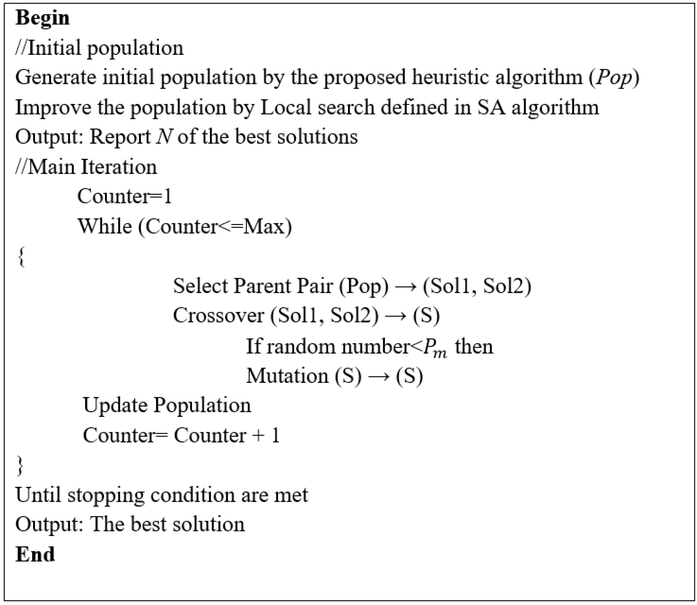
After reviewing the literature in different aspects, it is perceived that all of the research contains different solution methods so that each has its own advantages. Therefore, in this research, the most applied metaheuristic algorithms that is, SA and GA are combined together in order to keep the advantageous of each one. On the other hand, the applied local search procedures are defined innovatively in line with the problem solution space.

Accordingly, this research is aimed at presenting a novel model for the multi-trip CARP of urban waste collection which not only brings about economic benefits (minimizing the fixed cost of used vehicles) but also reduces adverse impacts of the CO₂ emission in air pollution considering advantages for the environment and people’s health. Also, a Hybrid Genetic Algorithm (HGA) is developed to solve the problem efficiently.

Therefore, the main novelties of the present paper are briefly as follows: (1) presentation of the multi-trip Green Capacitated Arc Routing Problem (G-CARP) which has not been yet introduced in the literature to the best of our knowledge; (2) since this paper is related to municipal solid waste management, loading, unloading sites and vehicle depots are commonly located in different places so that two separate locations are considered for the depot and unloading site in the model to make it closer to real world; and (3) developing a customized efficient solution method.

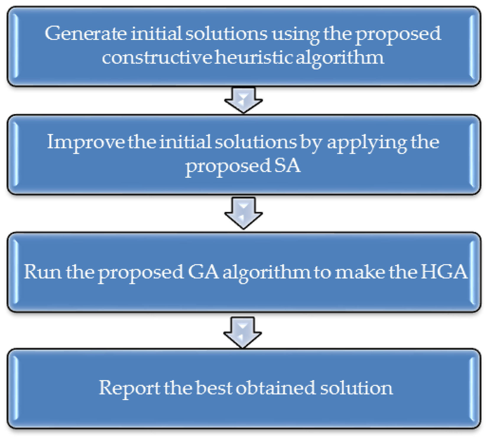
The remaining of the paper is organized as follows: Section 2 describes the distance-oriented green capacitated arc routing problem studied in this paper. Section 3 presents the proposed algorithm. Section 4 discusses the computational results. Finally, the concluding remarks and outlook of the research are presented in Section 5.

2. Distance-Oriented Green Capacitated Arc Routing Problem

The assessment of fuel consumption and CO₂ emission for vehicles requires performing complicated computations which only shows an estimation and approximation due to the difficulty of determining some of the fundamental variables values such as road slope, driving mode, weather conditions, accidents and so on [38].

The investigations performed on CO₂ emission are based on either fuel consumption or traveled distance. Based on an initiative approach of greenhouse gases protocol [39],

Table 1. Fuel-oriented and distance-oriented methods.

Fuel-based vs. Distance-based	Fuel-Oriented Method	Distance-Oriented Method
Advantages	More reliable	Easy to provide data
Disadvantages	Easy calculations only when fuel consumption data are available	High level of uncertainty
Data based on vehicle type	- Distance traveled - Fuel consumption factor - Heat values	- Distance traveled - Fuel consumption
Data gathering sources	- Fuel receipts - Fuel’s cost background - Direct measurement background, including official fuel consumption and tank gage records	- Odometer records - Company backgrounds on fuel economy data by a given vehicle
Emissions calculation	- Data calculation based on distance traveled by a given vehicle and fuel type - Converting the distance traveled to used fuel based on fuel economy data - Converting the fuel estimations to CO2 emissions by multiplying the used fuel by the fuel constant factors	- Data gathering based on distance traveled by a given vehicle and fuel type - Converting the distance estimations to CO2 emissions by multiplying the distance traveled by the distance-based emission factors

lists the required criteria for determining feasibility of each of these methods [39]. In one hand, in the fuel-oriented method, the fuel consumption is multiplied by CO₂ emission factor for the fuel type. On the other hand, in the distance-oriented method, CO₂ emission can be calculated using the distance-oriented emission factors. A fuel-oriented emission factor is developed based on fuel heat values, the fraction of fuel carbon which reacts with oxygen and carbon content coefficient. The distance-oriented method can be used when the data related to the traveled distance by the vehicle is available. Making a decision regarding which of these two methods is used, depends on the data accessibility.

It is clear that trying to obtain a theoretical formulation of this problem, the distance-oriented method (wherein CO₂ emission is calculated based on traveled distance and distance-based emission factors) is easier to apply. This requires taking two main steps: (1) collecting data on traveled distance by a given vehicle and fuel type (e.g., km or ton-km); and (2) converting the distance estimations to CO₂ emissions by multiplying the obtained results from step 1 by the distance-based emission factors.

In addition, the CO₂ emission calculations are based on the assumption that all of this computation depends mainly on two factors: type of the vehicle and type and quantity of the consumed fuel. Furthermore, this means that the emission is a function of two factors: transportation types (the vehicle and its load) and traveled distance [40]. Therefore, CO₂ emission estimations differ depending on the vehicle mass and transported load, which is an important parameter [41].

As it is presented in

Table 2. Estimated emission factor for a 10-ton truck [39].

Vehicle Status	Vehicle Load Percentage (%)	Consumption (Liter/100 km)	Fuel Conversion Factor (kg CO2/L)	Emission Factor (kg CO2/km)
Not loaded	0	29.6	2.61	0.733
Light loaded	25	32		0.831
Half loaded	50	34.4		0.9
Heavy loaded	75	36.7		0.958
Full loaded	100	39		1.018

, emission estimation factor goes through the two main steps mentioned earlier. The first step includes estimating a fuel conversion factor using chemical reaction of fuel combustion (C₁₃H₂₈ + 20 O₂ → 13 CO₂ + 14 H₂O) [42]. Given the molecular mass of diesel (C₁₃H₂₈) and CO₂ (184 and 24, respectively) and knowing that there are 13 CO₂ molecules for each diesel molecule, one can simply find that for each kg of diesel, 13 × 44/184 = 3.11 kg of CO₂ is produced. Then, using diesel density (0.84 kg/L), one can calculate the produced CO₂ per liter of consumed diesel (3.11 × 0.84 = 2.61 kg). It is observed that this estimated theoretical conversion factor is well close to that experimentally obtained by Defra (2.63 kg) [43], providing conversion factors for greenhouse gases, so as to use existing data resources and convert them to equivalent CO₂ emission data. Subsequently, having the fuel conversion factor (2.61 kg of CO₂/L of diesel), the second step is to estimate emission factor (ε). In this step, a function incorporating the data on average consumption depending on load is defined. Table 2 shows estimated value of this factor for several different capacity scenarios for a truck of 10 tons in capacity [39].

Accordingly, the presented information is generalized to our problem by considering the impact of CO₂ emission and conversion factors.

2.1. Mathematical Model of G-CARP in the Scope of Municipal Services

As the main difference between VRP and CARP, CARP consists of determining optimal routes that traverse all the edges with positive demands (required edges), however, VRP consists of finding optimal routes that traverse all the nodes defined in a graph network [1].

Consider a graph of G = (V, E) including the set of V for all the nodes constituting the edges and the set of E for all the edges defined in the network. The proposed G-CARP involves determining the optimal number of vehicles and optimal routes for each vehicle to minimize an overall objective function involving the cost of using the vehicles and the cost of total CO₂ emission throughout the network which has a direct relation with total traveled distance. The vehicles are originally located in depot; then start traveling (their first trip) to serve the required arcs and once their capacity limitation is reached, proceed to the unloading site to empty their loads. If possible, they continue traveling (their second trip) from the unloading site to the operational area. Having more than one trip for each vehicle directly depends on the capacity constraint and the maximum available time of vehicles. When the remaining time for a vehicle becomes zero, it shall return to the unloading site where it is unloaded before returning back to the depot.

Node 1 denotes the depot and node n denotes the unloading site in the network graph.

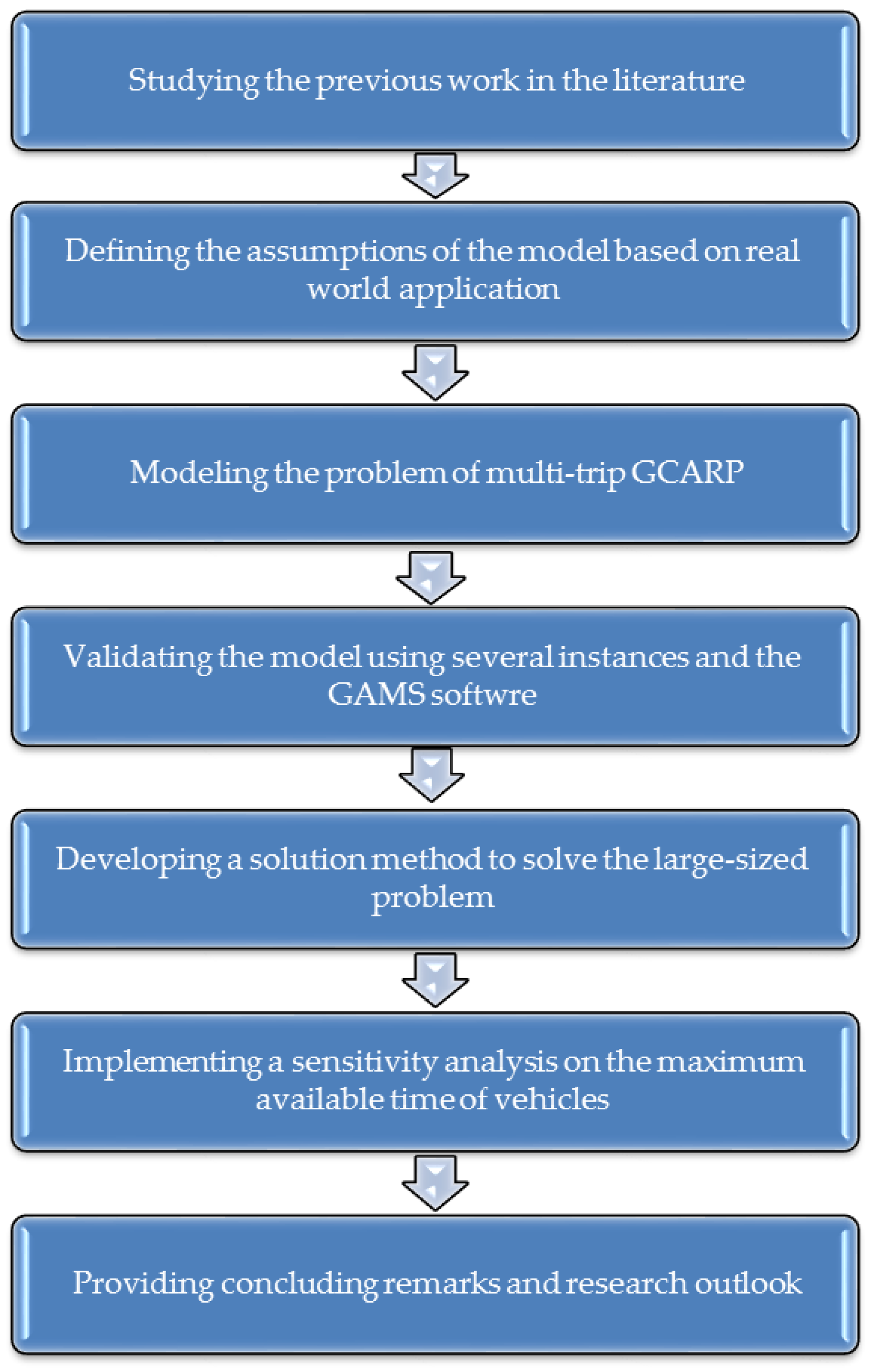
The main steps of the research and modeling the problem are described in Figure 1 before the model being presented.

Sets

V	The set of the network nodes
K	The set of the available vehicles
Pk	The set containing pth trip by the kth vehicle
E	The set of all edge defined across the network
ER	The set of all required edge defined in the network
S	An optional set of all edges defined in the network
V[S]	The set of nodes defined in the set S

Parameters

tij	The time it takes to traverse the edge (i, j), where (i, j) ∈ E
dij	Demand of the edge (i, j), where (i, j) ∈ E
cij	Distance (length) of the edge (i, j), where (i, j) ∈ E
eij	CO2 emission along the edge (i, j), where (i, j) ∈ E
Ψ	Cost conversion factor per CO2 emission unit
cvk	Cost of activating kth vehicle
Tmax	Maximum time available for each vehicle
Wk	Capacity of kth vehicle
G	A very large number

Decision variables

$$x_{ij{p}_k}=\{\begin{array}{c}\begin{array}{l}\mu \mathrm{If}\mathrm{the}\mathrm{edge}\left(i,j\right)\in E\mathrm{is}\mathrm{traveled}\mathrm{by}{k}^{\mathrm{t}\mathrm{h}}\mathrm{vehicle}\mathrm{in}\mathrm{the}{P}^{\mathrm{t}\mathrm{h}}\mathrm{trip}\mathrm{for}\mu \mathrm{times}(\mu \in Z^{+})\\ \end{array}\\ 0\mathrm{Otherwise}\end{array}$$

(1)

$$y_{ij{p}_k}=\{\begin{array}{c}\begin{array}{l}1\mathrm{If}\mathrm{the}\mathrm{edge}\left(i,j\right)\in E\mathrm{is}\mathrm{served}\mathrm{by}{k}^{\mathrm{t}\mathrm{h}}\mathrm{vehicle}\mathrm{in}\mathrm{the}{P}^{\mathrm{t}\mathrm{h}}\mathrm{trip}\\ \end{array}\\ 0\mathrm{Otherwise}\end{array}$$

(2)

$$u_k=\{\begin{array}{c}\begin{array}{l}1\mathrm{If}{k}^{\mathrm{t}\mathrm{h}}\mathrm{vehicle}\mathrm{is}\mathrm{used},\mathrm{where}k=1,\dots ,K\\ \end{array}\\ 0\mathrm{Otherwise}\end{array}$$

(3)

Mathematical model

$$\begin{gathered} Minimize Z1=\Psi \left({\displaystyle \sum }_{\left(i,j\right)\in E}{\displaystyle \sum }_{p_k\in P_k}^{}{\displaystyle \sum }_{k\in K}^{}{e}_{ij }{x}_{ij p_k}\right) \\ Minimize Z2={\displaystyle \sum }_{k\in K}^{}c{v}_k{u}_k \\ Minimize{Z}_{total}=Z1+Z2 \end{gathered}$$

(4)

s.t.

$${\displaystyle \sum }_{\left(i,j\right)\in E}^n{x}_{ij p_k}={\displaystyle \sum }_{\left(j,i\right)\in E}^n{x}_{j i p_k} \forall i\in V\backslash \left\{1,n\right\}, \forall k\in K,\forall p_k\in P_K,$$

(5)

$${\displaystyle \sum }_{p_k\in P_k}^{ }{\displaystyle \sum }_{k\in K}^{}\left(y_{ij p_k}^{ }+y_{j i p_k}^{ }\right)=1 \forall \left(i, j\right) or \left(j,i\right)\in E_R,$$

(6)

$${\displaystyle \sum }_{\left(i,j\right)\in E_R}^{ }{d}_{ij}{y}_{ij p_k}^{ }\le W_{k } \forall k\in K,\forall p_k\in P_K,$$

(7)

$$y_{i j p_k}\le x_{ij p_k} \forall \left(i,j\right)\in E_R, \forall k\in K, \forall p_k\in P_K,$$

(8)

$${\displaystyle \sum }_{p_k\in P_k}^{}{\displaystyle \sum }_{\left(i,j\right)\in E_{ }}{x}_{ij p_k}\le G u_k \forall k\in K,$$

(9)

$${\displaystyle \sum }_{p_k\in P_k}^{ }{\displaystyle \sum }_{\left(i,j\right)\in E_{ }}^{ }{t}_{ij}{x}_{ij p_k}\le T_{max } \forall k\in K,$$

(10)

$${\displaystyle \sum }_{\begin{array}{c}\left(1,j\right)\in E\\ j\in V\left\{1,n\right\}\end{array}}^{ }{x}_{1 j p_k}^{ } =u_k \forall k\in K,\forall p_k=1,$$

(11)

$${\displaystyle \sum }_{\begin{array}{c}\left(j,n\right)\in E\\ j\in V\left\{1,n\right\}\end{array}}^{ }{x}_{j n p_k}^{ } =u_k \forall k\in K,\forall p_k=1,$$

(12)

$${\displaystyle \sum }_{\begin{array}{c}\left(j,n\right)\in E\\ j\in V\left\{1,n\right\}\end{array}}^{ }{x}_{j n p_k}^{ } \le u_k \forall k\in K,\forall p_k\in \left\{2,\dots ,{P^{\prime }}_k\right\},$$

(13)

$${\displaystyle \sum }_{\begin{array}{c}\left(j,n\right)\in E\\ j\in V\left\{1,n\right\}\end{array}}^{ }{x}_{j n p_k}^{ } \le u_k \forall k\in K,\forall p_k\in \left\{2,\dots ,{P^{\prime }}_k\right\},$$

(14)

$${\displaystyle \sum }_{\left(j,h\right)\in S}^{ }{x}_{j h p_k}\le G {\displaystyle \sum }_{i\notin N\left[S\right], j\in N\left[S\right]}{x}_{ij p_k} \forall S\subseteq E, 1\notin V\left[S\right],\forall k\in K,\forall p_k\in P_K,$$

(15)

$$x_{ij p_k}\in Z^{+},y_{i j p_k}\in \left\{0,1\right\} ,u_k\in \left\{0,1\right\} \forall \left(i,j\right)\in E , \forall k\in K, \forall p_k\in P_K.$$

(16)

The objective function consists of two parts. The first part includes minimization of total CO₂ emission cost while the second part attempts to minimize the cost of using (renting) the k^th vehicle. Constraints (5) denote the flow balance for each vehicle, that is, it controls input to output from each intermediate node constituting two arcs. Constraint (6) ensures that each required edge is served by one of its two constituting arcs. Constraint (7) indicates the capacity constraint of the k^th vehicle. Constraint (8) expresses that the required edge is served by the vehicle traveling through it (or there are chances that a vehicle travels through an edge without having the edge served). Constraint (9) stipulates that the k^th vehicle will be used when the associated cost is paid. Constraint (10) represents the maximum time limitation considered for each vehicle. Constraints (11) and (12) ensure that the first trip of the vehicle starts from the depot and ends at unloading site. Constraints (13) and (14) make sure that from the second trip to the next (if any), the trips start and end at the unloading site. Constraint (15) ensures that no sub-tour will be constructed.

Total CO₂ emission is based on the environmental matrix (e) which is calculated by considering the matrix containing distances between each pair of nodes constituting edge (i, j) and respective emission factor (ε).

$$e_{ij}=c_{ij}\times \epsilon \left(d_{ij}\right), \forall \left(i, j\right)\in E$$

(17)

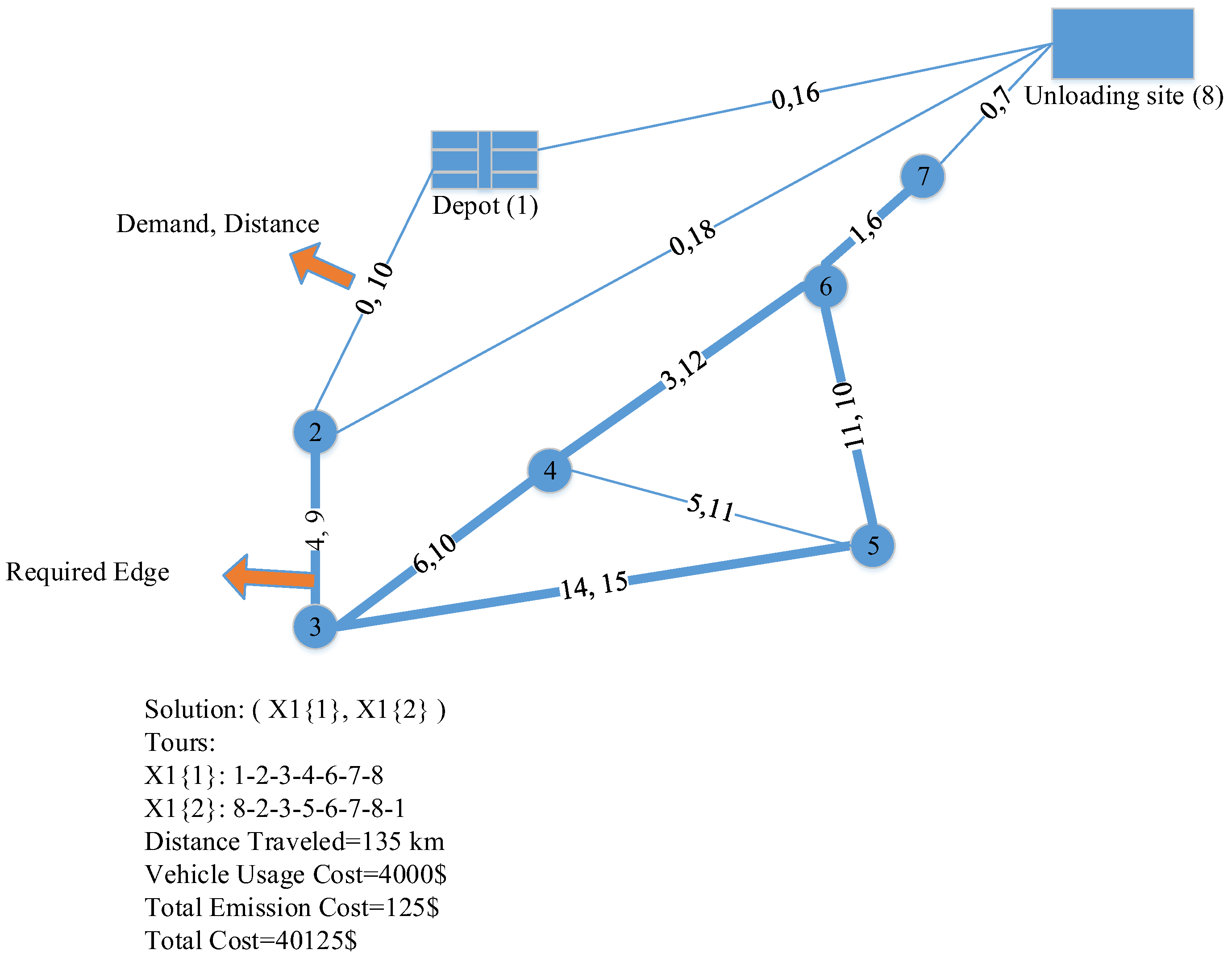
In order to gain a better understanding, an example with four required edges and two available vehicles is demonstrated in Figure 2. Nodes 1 and 8 represent the depot and unloading site, respectively. In this figure, the numbers indicated on each edge refer to the demand and length of the edge. It is assumed that the lengths of the edges are equal to their traversing time. The required edges are marked by solid lines (e.g., the edge (2, 3)). Vehicle 1 has the capacity of 40 units and the usage cost of 4000$. Vehicle 2 has the capacity of 50 units and the usage cost of 5000$. Maximum available time for each vehicle is equal to 200 units. In this example, vehicle 1 is used and constructs two trips in order to serve all the required edges.

By solving the final proposed model considering appropriate input parameter value and considering time periods, the obtained results will be reliable and applicable in an urban area and would definitely lead to huge cost savings as a real time application.

2.2. Limitations of the Adopted Model

The applicable limitations of the proposed adopted model are listed as below:

(1)

It is just applicable for a specific time period and it cannot include a planning horizon. As it is obvious the demand of different periods may be different and it would change the obtained results.

(2)

The exact fuel consumption rate is not accessible due to the hardness of computing the exact effects of the road slope, temperature conditions, load volume and so forth.

3. Hybrid Genetic Algorithm (HGA)

Since the CARP is an NP-Hard problem [9] and due to the high complexity of our proposed problem as an extended CARP, the exact methods are capable to solve the problem only in small sizes. Therefore, an HGA is proposed to solve the problem approximately in medium and large sizes. The proposed HGA is based on SA algorithm and Genetic Algorithm (GA).

The structure of the proposed HGA is depicted in Figure 3.

As it was mentioned, there are many applied metaheuristics presented in order to solve the optimization problems similar to the research problem [44,45,46,47,48,49]. Since the applicability and the robustness of the GA algorithms have been proved and it has generated appropriate solutions for CARPs in the literature [50,51,52,53,54], GA is proposed as the main algorithm for the current research.

In the following, the mechanism of the proposed algorithm is described.

In order to generate initial solutions for HGA, a heuristic initial solution generator algorithm is implemented. HGA is composed of three stages. In the first stage, a random solution is generated. The second stage involves improving the obtained solution by SA algorithm. In the third stage, GA is run with the output of the SA. In the HGA, the solution is represented by a chromosome as shown in

Table 3. The solution representation chromosome of the proposed HGA.

Description	Vehicle Number	Separator	Trip Number	Separator	Constructed Routes
First trip of the first vehicle	1	0	1	0	1- 2- 4- 5- 6- 7- 1
Second trip of the first vehicle	1	0	2	0	1- 3- 2- 4- 5- 7- 1
First trip of the second vehicle	2	0	1	0	1- 5- 3- 6- 4- 7- 1

.

3.1. Solution Representation

In the proposed algorithm, a matrix is used to represent the traversing sequence of the arcs, the related vehicle numbers and trip numbers in which there are two separators of number zero between vehicle number and trip number and between the trip number and constructed routes. According to the example presented in Table 3, we have two activated vehicles so that the first vehicle has two trips and the second one has only one trip that covers all the arcs with demands.

3.2. Initial Solution Heuristic Algorithm

In order to generate initial solutions, a constructive heuristic algorithm is employed. The steps taken in this algorithm are as follows:

• Select a vehicle randomly. The first trip starts at the depot.
• Among all of the edges starting at the depot, consider β edges with the shortest distance to the depot and select one of them randomly. Go to Step 3.
• Once arrived at the new vertex at the end of the selected edge, go to Step 4 if there exists any required edge; otherwise, go to Step 5.
• Among all of the required edges, consider β edges with the highest demands that can be selected considering vehicle capacity and maximum available time constraints. Select one of the β edges and go to Step 3. If there exists no required edge meeting both of the mentioned constraints, go to Step 5 (for an edge to meet the maximum available time constraint, there shall be a vehicle that can travel through the edge and then proceed to the unloading site within the specified time interval for the considered vehicle).
• Among the entire set of non-required edges at the considered vertex, select β edges meeting the time constraint with the smallest lengths and then select one of them randomly. If such conditions are not satisfied, go to the unloading site and then proceed to Step 6.
• If all of the required edges are served, go to Step 7, otherwise update the vehicle capacity constraint. If vehicle maximum available time constraint is at least enough to go from the unloading site through the shortest edge and then return to the unloading site, go to Step 3; otherwise, select the next vehicle and go to Step 2.
• Terminate the algorithm.

3.3. Improving the Solution Using SA Algorithm

SA algorithm is applied to improve the solutions and all of the initial solutions are separately improved using this algorithm. This algorithm has a great efficiency to solve the problems in non-convex or discrete solution space [55]. Initial parameters of the algorithm include the number of iterations at each temperature (M), initial temperature (TE₀), temperature reduction rate (α), ultimate temperature (TE_end) and Boltzmann’s constant (Kc), which are initialized before starting to search. Then, a neighborhood of the initial solution is considered. If the value of the objective function within the generated neighborhood is better than the value of the objective function for the respective initial solution, the neighborhood replaced the initial solution; otherwise, a random number between zero and one was generated and compared to the algorithm defined equation [45]. If the random number is smaller than the value of the algorithm equation, the worse solution is accepted. A number of iterations were performed at each temperature before going to a lower temperature. Stopping criterion is set for achieving the ultimate temperature. In the present paper, the values of the algorithm parameters are set as follows using trial-and-error method wherein three example problems are solved under different scenarios to find the best values of the algorithm parameters.

M = 5, α = 0.98, TE₀ = 200, TE_end = 1, Kc = 0.8

(18)

Local search methods applied in this algorithm are as follows:

• Swap a trip of one vehicle with a trip of another vehicle at random. A solution can be a candidate for selection only if it is viable.
• Two trips are selected at random. If there exists common edge/edges in the two selected trips, one of the edges is selected randomly and both of the trips are divided into two parts considering the selected edge. The first part of the first trip is combined with the second part of the second trip and the first part of the second trip is combined with the second part of the first trip to form two new trips.
• Two trips are selected at random. If there exists common edge/edges in the two selected trips, the sequence between common edges of the two trips is changed.
• One edge along one trip is selected randomly and its direction is reversed.
• Part of a trip is selected at random and its direction is reversed.

3.4. Genetic Algorithm

This algorithm is based on producing new generations and selecting the best solutions for producing the next generation [56]. The heuristic approach explained earlier is used to generate initial solutions and to be improved by SA for the proposed GA. For this purpose, the heuristic algorithm generates a specified number of initial solutions (200 solutions). Among the generated solutions, a sample of the size equal to that of the initial population of the GA is taken following the initial solution selection approach explained in the next sub-section. In the next stage, the required number of solutions is selected using two-parent tournament selection method and the proposed crossover method explained in the following is employed to generate two solutions. This process is repeated until the required number of solutions is achieved, followed by applying mutation operator at a particular rate following the method proposed in the following. Finally, among all of the solutions, a specified number of solutions are selected via the initial solution method and transferred to the next generation, eliminating all other solutions.

3.4.1. Initial Solution Selection

Two things must be considered when selecting initial solutions. The first thing to consider is the quality of solutions and the second thing is the scattering of the solutions. If one focuses on selecting the best solutions only, the search space will be reduced and there are chances of trapping in local minima. In order to address this problem, the present paper proposes an initial solution selection approach which goes through the following steps:

• Define two sets Q and S, which are initially empty.
• Assign the initially generated solutions to the Set Q and sort them by the value of the objective function (ascending).
• Divide the interval between the best and worst values of the objective function into num intervals of the same length (where num is the number of solutions to be selected).
• Select isolated solutions in each interval and transfer them to the set S before having them eliminated from the set Q. If the number of selected solutions is equal to n, terminate the algorithm; otherwise, proceed to Step 5.
• Assign a value to the solutions remaining in set Q. The value is equal to the inverse of the number of the solutions within the respective interval of solutions.
• Sort the solutions by value (descending) and assign to each solution a cumulative score obtained by summing up scores of previous solutions and that of the current solution. Each time, generate a random number between zero and the sum of scores, select the solution which falls within the considered interval and transfers it to the set S.
• If the set S contains enough number of initial solutions, terminate the algorithm; otherwise, go to Step 6.

3.4.2. GA Operators

The most important operator in the scope of a GA is crossover operator. The proposed crossover operation is as follows:

• Two parents are selected via tournament method. For this purpose, a particular number of solutions are selected randomly and the two ones for which the best values of the objective function is obtained are selected. Two trips are selected at random and swapped between the two parents.
• Two parents are selected via tournament method, from whom two trips are selected randomly. If there exists common edge/edges in the two selected trips, one of the edges is selected randomly and both of the trips are divided into two parts considering the selected edge. The first part of the first trip is combined with the second part of the second trip and the first part of the second trip is combined with the second part of the first trip to form two new trips to replace the previous trips.

On the other hand, the mutation operator is applied at the fixed rate of Pm to mutate the child produced via the crossover operation.

The local search methods used to improve initial solutions is further used as mutation operators.

After applying the operators, the feasibility of the solutions are evaluated by the existence check of the arcs in the graph network, vehicle capacity constraint of each trip, vehicle maximum available time in each tour.

3.4.3. Parameter Tuning of the HGA

In order to adjust the parameters of the proposed HGA, a trial-and-error approach is followed, wherein three example problems are solved under different scenarios to find the best values of the algorithm parameters. Considering what has mentioned above, the number of initial solutions generated by the proposed heuristic algorithm is set to 200 (i.e., initial population size), the number of solutions obtained from the crossover operator is set to 150 and mutation rate is set to 0.1. Figure 4 demonstrates pseudo-code of the proposed GA.

4. Numerical Results

In this section, in order to validate the proposed mathematical model and to evaluate the performance of the proposed algorithm, 15 random instances of various sizes are generated. After solving instances with the exact method and analyzing the obtained results, it has been revealed that the proposed model has passed its validity test.

For all of the instances, two types of vehicle (types 1 and 2) with capacities and activation costs of 5 and 7 tons and 400$ and 500$, respectively, were considered. Supporting information and network structure are demonstrated in

Table 4. Input information of the instances.

Instances	TE	RE	AV1	AV2
P1	8	6	1	1
P2	20	16	2	1
P3	35	28	2	2
P4	50	33	4	3
P5	70	49	4	4
P6	90	52	6	5
P7	100	62	7	6
P8	120	78	8	7
P9	140	85	9	7
P10	150	96	10	8
P11	190	123	10	9
P12	200	129	11	9
P13	230	153	12	10
P14	250	197	12	11
P15	280	214	13	11
P16	310	246	15	13
P17	330	265	16	15
P18	400	320	18	16

TE: total edges; RE: total required edges; AV1: total available vehicles type 1; AV2: total available vehicles type 2.

. The input parameters values are generated randomly with a uniform distribution.

In Table 4, column 1 denotes the instance number, column 2 defines the total number of edges, column 3 gives the number of required edges and columns 4 and 5 show numbers of available vehicles of types 1 and 2, respectively, for each instance. The emission factors of the vehicles are described in

Table 5. Estimated emission factor for the 5-ton and 7-ton trucks.

Vehicle Status	ε of a 5-ton Vehicle	ε of a 7-ton Vehicle
Not loaded	0.535	0.638
Light loaded	0.607	0.723
Half loaded	0.657	0.783
Heavy loaded	0.699	0.833
Full loaded	0.743	0.886

. Also, Ψ is equal to 10 in all instances.

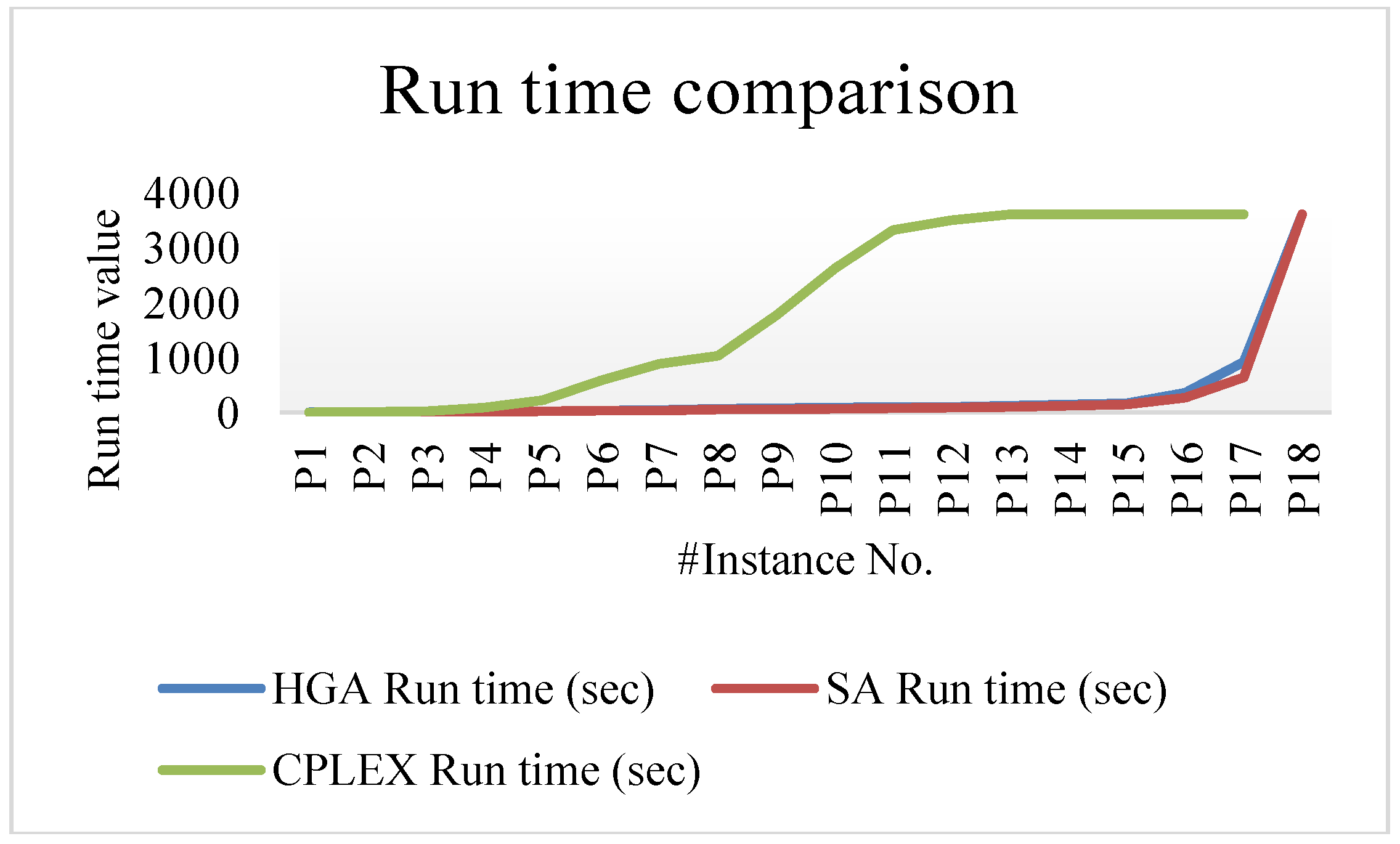
The 15 instances are then solved using CPLEX solver of GAMS Software, the proposed SA and HGA separately for the applied run time constraint of 3600 s. The aim of investigating SA and HGA separately is to make the impact of applying GA on SA more obvious. In fact, HGA is the result of applying GA on SA.

The obtained results are shown in Table 5. The solution methods are executed on a Laptop equipped with Core i7 CPU @ 2.60 GHz processor and 12.00 GB of RAM.

As it is obvious in

Table 6. The obtained computational results.

Instances	CPLEX Objective	SA	HGA	CPLEX Run Time (s)	SA Run Time (s)	HGA Run Time (s)	SA Gap (%)	HGA Gap (%)
		Objective	Objective
P1	1122.17	1130.47	1129.13	3.5	2.18	4.49	0.74	0.62
P2	1542.23	1557.34	1556.11	9.32	4.83	6.4	0.98	0.9
P3	1624.24	1653.8	1651.85	21.12	8.97	11.12	1.82	1.7
P4	3285.49	3364.34	3338.06	90.33	16.1	22.17	2.4	1.6
P5	3780.57	3878.11	3857.32	221.58	19.84	25.05	2.58	2.03
P6	4891.73	5071.26	5008.64	584.23	29.55	38.78	3.67	2.39
P7	5875.88	6076.25	6003.97	887.82	36.04	45.24	3.41	2.18
P8	6720.01	6917.58	6853.07	1030.68	54.65	68.02	2.94	1.98
P9	7057.06	7342.87	7198.91	1765.14	57.23	75.09	4.05	2.01
P10	7537.13	7829.57	7728.57	2620.02	65.17	87.84	3.88	2.54
P11	8004.2	8305.16	8163.48	3315.32	74.26	98.23	3.76	1.99
P12	8734.31	9135.21	8967.52	3492.1	89.1	101.3	4.59	2.67
P13	8985.35	9360.94	9176.74	3600	101.21	121.36	4.18	2.13
P14	9350.4	9651.48	9485.98	3600	128.06	142.02	3.62	1.45
P15	10,044.5	10,024.51	9842.16	3600	143.84	163.19	0	0
P16	- *	14,680.5	14,459.78	3600	268.11	354.85	0	0
P17	- *	18,526.22	18,268.38	3600	642.58	923.07	-	-
P18	- *	- *	- *	3600	3600	3600	-	-
Average	-	-	-	1980.06	296.76	327.12	2.66	1.64

* No solution found.

, CPLEX is not capable of finding a solution for some problems by applying the 3600 s run time limitation. Results have shown that the proposed HGA has appropriate efficiency in comparison with SA and CPLEX. However, SA could solve the problems at a lower run time against HGA, however, this difference is negligible due to the significant better Gap percentage (Figure 5). The average gaps obtained by SA and HGA are 2.66% and 1.64%, respectively. On the other hand, the capability of the proposed solution methods is evaluated through solving P15–P18. As it is obvious, CPLEX could report the best found solution up to the first 15 problems. For P16–P17, there is a significant increase in run time of SA and HGA and for P18, none of the algorithms are able to find any solution within 3600 run time limitation. It shows that some additional modification may be needed to be applied to improve the efficiency of for solving very large sized problems. The number of used vehicles in each instance problems is presented in

Table 7. The number of used vehicles obtained by different solution methods.

Instances	Solution by CPLEX		Solution by SA		Solution by HGA
	UV1 *	UV2 **	UV1	UV2	UV1	UV2
P1	1	1	1	1	1	1
P2	2	1	2	1	2	1
P3	2	1	2	1	2	1
P4	3	3	3	3	3	3
P5	4	3	4	3	4	3
P6	6	4	5	5	6	4
P7	6	6	6	6	6	6
P8	8	5	7	6	7	6
P9	8	6	7	7	8	6
P10	8	7	8	7	9	6
P11	9	7	8	8	8	8
P12	9	8	8	9	8	9
P13	10	8	9	9	10	8
P14	11	8	10	9	10	9
P15	10	10	12	8	11	9
P16	-	-	13	13	14	12
P17	-	-	14	14	14	14
Average of P1–P15	6.47	5.2	6.13	5.53	6.33	5.33

* The number of used vehicle type 1; ** The number of used vehicle type 2.

for different solution methods. As it is obvious, there are no significant differences between the number of used vehicle types 1 and 2.

As another advantage of the proposed algorithm, it can solve the large sized problems with a reasonable low run time in comparison with the algorithms proposed in the literature like Improved Max-Min Ant System (IMMAS) [1].

Sensitivity Analysis

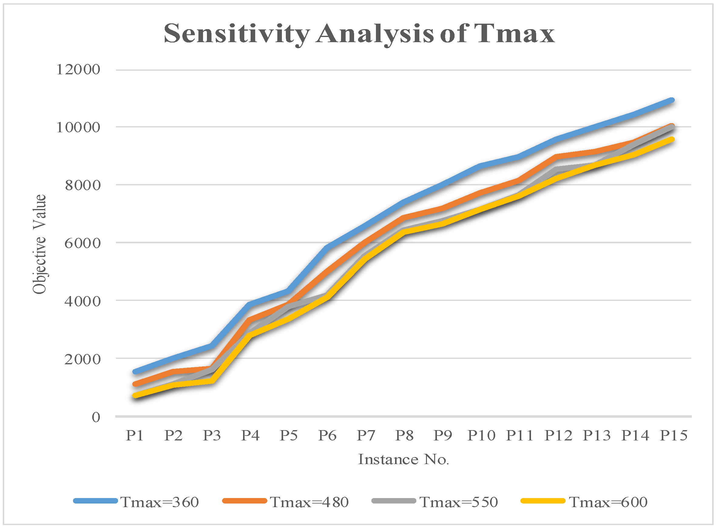
In order to investigate the effects of changing some parameters on the value of the objective function, a sensitivity analysis is performed on these parameters of the first fifteen problems by HGA. In fact, the behavior of the objective is studied in front of the uncertain environment if the considered value of a parameter changed. On the other hand, managers are willing to know how much benefits would be gained if they assign more resources. In fact, they want to know about the relation defined between objective function and the value of the assigned resources. In this research, the effects of the maximum available time of each vehicle on the objective are analyzed. Four different executive values (i.e., 360, 480, 550 and 600 min) are considered for the parameter while the other parameters are constant.

Results of the sensitivity analysis on Tmax are given in

Table 8. Computational results obtained for different values of Tmax.

Instances	Tmax
	360	480	550	600
P1	1559.26	1129.13	715.54	715.54
P2	2013.64	1556.11	1110.09	1067.3
P3	2442.06	1651.85	1617.46	1221.36
P4	3865.33	3338.06	2881.21	2817.07
P5	4358.89	3857.32	3798.14	3362.25
P6	5830.27	5008.64	4214.08	4137.92
P7	6600.23	6003.97	5544.95	5466.78
P8	7424	6853.07	6459.62	6392.9
P9	8029.31	7198.91	6787.7	6682.46
P10	8673.69	7728.57	7182.48	7182.48
P11	9015.43	8163.48	7687.57	7651.06
P12	9605.97	8967.52	8552.43	8234.75
P13	10,036.13	9176.74	8727.81	8719.29
P14	10,479.59	9485.98	9418.3	9077.57
P15	10,965.77	9842.16	9654.11	9615.73
Average	6712.133	6010.06	5636.13	5477.86

. The most important conclusion drawn from the analysis is that the higher the Tmax is, the lower objective function and the lower number of the used vehicles are.

As it is clear in Figure 6, the objective value will increase significantly by changing Tmax to 360 min. In other words, the worst case is obtained by Tmax of 360. The difference between the objective values obtained by Tmax of 550 and 600 is proportionally the lowest.

Table 9. Cost savings obtained for different values of Tmax.

Instances	Tmax
	360	550	600
P1	−430.13	413.59	413.59
P2	−457.53	446.02	488.81
P3	−790.21	34.39	430.49
P4	−527.27	456.85	520.99
P5	−501.57	59.18	495.07
P6	−821.63	794.56	870.72
P7	−596.26	459.02	537.19
P8	−570.93	393.45	460.17
P9	−830.4	411.21	516.45
P10	−945.12	546.09	546.09
P11	−851.95	475.91	512.42
P12	−638.45	415.09	732.77
P13	−859.39	448.93	457.45
P14	−993.61	67.68	408.41
P15	−1123.61	188.05	226.43
Average cost saving	−729.2	374	507.8

shows the cost savings obtained by different Tmax value.

In order to optimize associated costs, managers should consider the impact of these maximum vehicle usage times and set an appropriate upper limit to gain maximum cost saving. As it is presented in Table 9, the average cost saving for Tmax of 360 is not a positive value that is, it causes the loss for all instances. The average cost savings for Tmax of 550 and 600 are equal to 374.00 and 507.80, respectively. Finally, the performed sensitivity analysis can be used as a managerial tool to be applicable in decision making processes.

5. Conclusions

Considering economic and environmental aspects of the urban services are two inseparable parts of decision making in the organizations such as municipalities. Usually, these two important factors are investigated separately in applied research. This has been while, in many cases, finding the shortest routes could not result in optimal solution when CO₂ emission and air pollution minimization is taken as the objective function, because fuel consumption depends on many factors including the vehicle load, speed, road conditions and so forth. In this paper, a multi-trip Green Capacitated Arc Routing Problem is proposed to find the shortest routes serving to minimize total cost and total emission of greenhouse gases considering various types of real world constraints, such as capacity constraint, maximum available time for vehicles and so forth. In other words, the aim is to reduce adverse impacts of greenhouse gases and air pollution besides further consideration of cost minimization in terms of the minimal activation of vehicle fleet for serving waste and the optimal routing. In order to solve the proposed model, a hybrid genetic algorithm is developed based on a simulated annealing algorithm and genetic algorithm. The results indicated the high efficiency of the proposed algorithm so that it could yield solutions with the average gap of 1.64% for the instances. On the other hand, the proposed HGA solve large sized problems in an appropriate run time in comparison with the other algorithms proposed in the literature. Finally, a sensitivity analysis is implemented on the problem to study the impact of different maximum available time of vehicles and propose the optimal policies. For future studies, it is proposed to develop the robust optimization approaches for the problem in order to evaluate the effect of uncertainty. On the other hand, proposing another novel algorithm such as polar bear optimization and moth-flame optimization would be effective in order to test the proposed algorithm in large sized problems.

References

1. Tirkolaee, E.B.; Alinaghian, A.; Hosseinabadi, A.A.R.; Sasi, M.B.; Sangaiah, A.K. An improved ant colony optimization for the multi-trip Capacitated Arc Routing Problem. Comput. Electr. Eng. 2018. [Google Scholar] [CrossRef]
2. Tirkolaee, E.B.; Goli, A.; Bakhsi, M.; Mahdavi, I. A robust multi-trip vehicle routing problem of perishable products with intermediate depots and time windows. Numer. Algebra Control Optim. 2017, 7, 417–433. [Google Scholar]
3. Wang, J.; Cao, Y.Q.; Li, B.; Kim, H.J.; Lee, S.Y. Particle Swarm Optimization based Clustering Algorithm with Mobile Sink for WSNs. Future Gener. Comput. Syst. 2017, 76, 452–457. [Google Scholar] [CrossRef]
4. Alinaghian, M.; Amanipour, H.; Tirkolaee, E.B. Enhancment of Inventory Management Approaches in Vehicle Routing-Cross Docking Problems. J. Supply Chain Manag. Syst. 2014, 3, 27–34. [Google Scholar]
5. Mirmohammadi, S.H.; Babaee Tirkolaee, E.; Goli, A.; Dehnavi-Arani, S. The periodic green vehicle routing problem with considering of the time-dependent urban traffic and time windows. Iran Univ. Sci. Technol. 2017, 7, 143–156. [Google Scholar]
6. Baidu Index. 2017. Available online: https://index.baidu.com/ (accessed on 21 August 2017).
7. Xiao, Y.; Konak, A. Green vehicle routing problem with time-varying traffic congestion. In Proceedings of the 14th INFORMS Computing Society Conference, Richmond, Virginia, 11–13 January 2015; pp. 134–148. [Google Scholar]
8. Golden, B.L.; Assad, A.A.; Wasil, E.A. Routing Vehicles in the Real World: Applications in the Solid Waste, Beverage, Food, Dairy and Newspaper Industries. In The Vehicle Routing Problem; Toth, P., Vigo, D., Eds.; Society for Industrial and Applied Mathematics: Philadelphia, PA, USA, 2002; pp. 245–286. [Google Scholar]
9. Golden, B.; Wong, R. Capacitated arc routing problems. Networks 1981, 11, 305–315. [Google Scholar] [CrossRef]
10. Dror, M. ARC ROUTING: Theory, Solutions and Applications; Kluwer Academic Publishers: Dordrecht, The Netherlands, 2000. [Google Scholar]
11. Assad, A.A.; Golden, B.L. Arc routing methods and applications. In Handbooks in Operations Research and Management Science; Elsevier: New York, NY, USA, 1995; Volume 8, pp. 375–483. [Google Scholar]
12. Ghiani, G.; Laganà, D.; Laporte, G.; Mari, F. Ant colony optimization for the arc routing problem with intermediate facilities under capacity and length restrictions. J. Heuristics 2010, 16, 211–233. [Google Scholar] [CrossRef]
13. Li, J.; Borenstein, D.; Mirchandania, P.B. Truck scheduling for solid waste collection in the city of Porto Alegre, Brazil. Omega-Int. J. Manag. Sci. 2008, 36, 1133–1149. [Google Scholar] [CrossRef]
14. Laporte, G.; Musmanno, R.; Vocaturo, F. An adaptive large neighbourhood search heuristic for the capacitated arc-routing problem with stochastic demands. Transp. Sci. 2010, 44, 125–135. [Google Scholar] [CrossRef]
15. Khosravi, P.; Alinaghian, M.; Sajadi, S.; Babaee, E. The Periodic Capacitated Arc Routing Problem with Mobile Disposal Sites Specified for Waste Collection. J. Appl. Res. Ind. Eng. 2015, 2, 64–76. [Google Scholar]
16. Babaee Tirkolaee, E.; Alinaghian, M.; Bakhshi Sasi, M.; Seyyed Esfahani, M.M. Solving a robust capacitated arc routing problem using a hybrid simulated annealing algorithm: A waste collection application. J. Ind. Eng. Manag. Stud. 2016, 3, 61–76. [Google Scholar]
17. Hannan, M.A.; Akhtar, M.; Begum, R.A.; Basri, H.; Hussain, A.; Scavino, E. Capacitated vehicle-routing problem model for scheduled solid waste collection and route optimization using PSO algorithm. Waste Manag. 2018, 71, 31–41. [Google Scholar] [CrossRef] [PubMed]
18. Rey, A.; Prieto, M.; Gómez, J.I.; Tenllado, C.; Hidalgo, J.I. A CPU-GPU Parallel Ant Colony Optimization Solver for the Vehicle Routing Problem. In Proceedings of the International Conference on the Applications of Evolutionary Computation, Parma, Italy, 4–6 April 2018; Springer: Cham, Switzerland, 2018; pp. 653–667. [Google Scholar]
19. Tirkolaee, E.B.; Mahdavi, I.; Esfahani, M.M.S. A robust periodic capacitated arc routing problem for urban waste collection considering drivers and crew’s working time. Waste Manag. 2018, in press. [Google Scholar] [CrossRef] [PubMed]
20. Lin, C.; Choy, K.L.; Ho, G.T.; Chung, S.H.; Lam, H.Y. Survey of green vehicle routing problem: Past and future trends. Expert Syst. Appl. 2014, 41, 1118–1138. [Google Scholar] [CrossRef]
21. Maden, W.; Eglese, R.W.; Black, D. Vehicle routing and scheduling with time varying data: A case study. J. Oper. Res. Soc. 2010, 61, 515–522. [Google Scholar] [CrossRef] [Green Version]
22. Erdoğan, S.; Miller-Hooks, E. A green vehicle routing problem. Transp. Res. Part E Logist. Transp. Rev. 2012, 48, 100–114. [Google Scholar] [CrossRef]
23. Kopfer, H.W.; Schönberger, J.; Kopfer, H. Reducing greenhouse gas emissions of a heterogeneous vehicle fleet. Flex. Serv. Manuf. J. 2014, 26, 221–248. [Google Scholar] [CrossRef]
24. Tavares, G.; Zsigraiova, Z.; Semiao, V.; da Grac, M. A case study of fuel savings through optimization of MSW transportation routes. Manag. Environ. Qual. Int. J. 2008, 19, 444–454. [Google Scholar] [CrossRef]
25. Çimen, M.; Soysal, M. Time-dependent green vehicle routing problem with stochastic vehicle speeds: An approximate dynamic programming algorithm. Transp. Res. Part D Transp. Environ. 2017, 54, 82–98. [Google Scholar] [CrossRef]
26. Rabbani, M.; Bosjin, S.; Yazdanparast, R.; Saravi, N. A stochastic time-dependent green capacitated vehicle routing and scheduling problem with time window, resiliency and reliability: A case study. Decis. Sci. Lett. 2018, 7, 381–394. [Google Scholar] [CrossRef]
27. Poonthalir, G.; Nadarajan, R. A Fuel Efficient Green Vehicle Routing Problem with varying speed constraint (F-GVRP). Expert Syst. Appl. 2018, 100, 131–144. [Google Scholar] [CrossRef]
28. Kulkarni, S.; Patil, R.; Krishnamoorthy, M.; Ernst, A.; Ranade, A. A new two-stage heuristic for the recreational vehicle scheduling problem. Comput. Oper. Res. 2018, 91, 59–78. [Google Scholar] [CrossRef]
29. Wang, J.; Cao, J.; Ji, S.; Park, J.H. Energy Efficient Cluster-based Dynamic Routes Adjustment Approach for Wireless Sensor Networks with Mobile Sinks. J. Supercomput. 2017, 73, 3277–3290. [Google Scholar] [CrossRef]
30. Wang, J.; Yang, X.; Li, B.; Lee, S.Y.; Jeon, S. A mobile sink based uneven clustering algorithm for wireless sensor networks. J. Internet Technol. 2013, 14, 895–902. [Google Scholar]
31. Wang, J.; Li, B.; Xia, F.; Kim, C.; Kim, J.U. An Energy Efficient Distance-Aware Routing Algorithm with Multiple Mobile Sinks for Wireless Sensor Networks. Sensors 2013, 14, 15163–15181. [Google Scholar] [CrossRef] [PubMed]
32. Ou, T.C.; Hong, C.M. Dynamic operation and control of microgrid hybrid power systems. Energy 2014, 66, 314–323. [Google Scholar] [CrossRef]
33. Ou, T.C.; Lu, K.H.; Huang, C.J. Improvement of transient stability in a hybrid power multi-system using a designed NIDC (Novel Intelligent Damping Controller). Energies 2017, 10, 488. [Google Scholar] [CrossRef]
34. Ou, T.C. Design of a Novel Voltage Controller for Conversion of Carbon Dioxide into Clean Fuels Using the Integration of a Vanadium Redox Battery with Solar Energy. Energies 2018, 11, 524. [Google Scholar] [CrossRef]
35. Uebel, S.; Murgovski, N.; Tempelhahn, C.; Bäker, B. Optimal Energy Management and Velocity Control of Hybrid Electric Vehicles. IEEE Trans. Veh. Technol. 2017, 67, 327–337. [Google Scholar] [CrossRef]
36. Woźniak, M.; Połap, D. Hybrid neuro-heuristic methodology for simulation and control of dynamic systems over time interval. Neural Netw. 2017, 93, 45–56. [Google Scholar] [CrossRef] [PubMed]
37. Alcala, E.; Puig, V.; Quevedo, J.; Escobet, T.; Comasolivas, R. Autonomous vehicle control using a kinematic Lyapunov-based technique with LQR-LMI tuning. Control Eng. Pract. 2018, 73, 1–12. [Google Scholar] [CrossRef]
38. Palmer, A. An integrated routing model to estimate carbon dioxide emissions from freight vehicles. In Logist Res Network Conference Proceedings; Lalwani, C., Mangan, J., Butcher, T., Coronado-Mondragon, A., Eds.; University of Hull: Hull, UK, 2007; pp. 27–32. [Google Scholar]
39. Úbeda, S.; Faulin, J.; Serrano, A.; Arcelus, F.J. Solving the green capacitated vehicle routing problem using a tabu search algorithm. Lect. Notes Manag. Sci. 2014, 6, 141–149. [Google Scholar]
40. Ferreti, I.; Zanoni, S.; Zavanella, L.; Diana, A. Greening the aluminium supply chain. Int. J. Prod. Econ. 2007, 108, 236–245. [Google Scholar] [CrossRef]
41. McKinnon, A. CO2 emissions from freight transport: An analysis of UK data. In Logist Res Network Conference Proceedings; Lalwani, C., Mangan, J., Butcher, T., Coronado-Mondragon, A., Eds.; University of Hull: Hull, UK, 2007; pp. 9–14. [Google Scholar]
42. Lichty, L.C. Combustion Engine Processes; McGraw-Hill Education: New York, NY, USA, 1967. [Google Scholar]
43. Kenny, T.; Gray, N.F. Comparative performance of six carbon footprint models for use in Ireland. Environ. Impact Assess. Rev. 2009, 29, 1–6. [Google Scholar] [CrossRef]
44. Hosseinabadi, A.R.; Kardgar, M.; Shojafar, M.; Shamshirband, S.; Abraham, A. Gravitational Search Algorithm to Solve Open Vehicle Routing Problem. In Proceedings of the 6th International Conference on Innovations in Bio-Inspired Computing and Applications, Chapter Advances in Intelligent Systems and Computing, Kochi, India, 16–18 December 2015; Springer: Berlin, Germany, 2015; pp. 93–103. [Google Scholar]
45. Shamshirband, S.; Shojafar, M.; Hosseinabadi, A.R.; Abraham, A. OVRP_ICA: An Imperialist-based Optimization Algorithm for the Open Vehicle Routing Problem. In Proceedings of the International Conference on Hybrid Artificial Intelligence Systems (HAIS), Bilbao, Spain, 22–24 June 2015; Springer: Berlin, Germany, 2015. Chapter Springer LNCS. Volume 9121, pp. 221–233. [Google Scholar]
46. Hosseinabadi, A.R.; Kardgar, M.; Shojafar, M.; Shamshirband, S.; Abraham, A. GELS-GA: Hybrid Metaheuristic Algorithm for Solving Multiple Travelling Salesman Problem. In Proceedings of the IEEE International Conference on Intelligent Systems Design and Applications (ISDA), Okinawa, Japan, 28–30 November 2014; pp. 76–81. [Google Scholar]
47. Hosseinabadi, A.R.; Vahidi, J.; Balas, V.E.; Mirkamali, S.S. OVRP_GELS: Solving Open Vehicle Routing Problem Using the Gravitational Emulation Local Search Algorithm. Neural Comput. Appl. 2016, 29, 955–968. [Google Scholar] [CrossRef]
48. Hosseinabadi, A.R.; Rostami, N.S.H.; Kardgar, M.; Mirkamali, S.S.; Abraham, A. A New Efficient Approach for Solving the Capacitated Vehicle Routing Problem Using the Gravitational Emulation Local Search Algorithm. Appl. Math. Model. 2017, 49, 663–679. [Google Scholar] [CrossRef]
49. Hosseinabadi, A.R.; Alavipour, F.; Shamshirbnd, S.; Balas, V.E. A Novel Meta-Heuristic Combinatory Method for Solving Capacitated Vehicle Location-Routing Problem with Hard Time Windows. In Transportation Systems, Advances in Intelligent Systems and Computing; Springer International Publishing: Cham, Switzerland; Beijing, China, 2017; Volume 454, pp. 707–728. [Google Scholar]
50. Fleury, G.; Lacomme, P.; Prins, C. Evolutionary algorithms for stochastic arc routing problems. In Applications of Evolutionary Computing; Springer: Berlin/Heidelberg, Germany, 2004; pp. 501–512. [Google Scholar]
51. Lacomme, P.; Prins, C.; Ramdane-Chérif, W. A genetic algorithm for the capacitated arc routing problem and its extensions. In Workshops on Applications of Evolutionary Computation; Springer: Berlin/Heidelberg, Germany, 2001; pp. 473–483. [Google Scholar]
52. Lacomme, P.; Prins, C.; Sevaux, M. A genetic algorithm for a bi-objective capacitated arc routing problem. Comput. Oper. Res. 2006, 33, 3473–3493. [Google Scholar] [CrossRef]
53. Lacomme, P.; Prins, C.; Ramdane-Chérif, W. Evolutionary algorithms for periodic arc routing problems. Eur. J. Oper. Res. 2005, 165, 535–553. [Google Scholar] [CrossRef]
54. Corberán, A.; Prins, C. Recent results on arc routing problems: An annotated bibliography. Networks 2010, 56, 50–69. [Google Scholar] [CrossRef]
55. Glover, F.W.; Kochenberger, G. Handbook of Metaheuristics; Kluwer Academic Publishers: Norwell, MA, USA, 2005. [Google Scholar]
56. Holland, J.H. Adaptation in Natural and Artificial Systems: An Introductory Analysis with Applications to Biology, Control, and Artificial Intelligence; University of the Michigan Press: Ann Arbor, MI, USA, 1975. [Google Scholar]
Figure 1. The main steps of the research.
Sustainability 10 01366 g001
Figure 2. A schematic example and solution generation flow.
Sustainability 10 01366 g002
Figure 3. The structure of the proposed hybrid genetic algorithm (HGA).
Sustainability 10 01366 g003
Figure 4. The proposed HGA pseudo-code.
Sustainability 10 01366 g004
Figure 5. A comparison of computational times between CPLEX solver, SA and HGA.
Sustainability 10 01366 g005
Figure 6. A comparison between mean values of the objective function for different values of Tmax.
Sustainability 10 01366 g006