Article

Study on Air Pollution and Control Investment from the Perspective of the Environmental Theory Model: A Case Study in China, 2005–2014

1
College of Geography and Environmental Sciences, Zhejiang Normal University, Jinhua 321004, Zhejiang, China
2
Remote Sensing Application & Environmental Disaster Research Center, Zhejiang Normal University, Jinhua 321004, Zhejiang, China
3
College of Foreign Languages, Zhejiang Normal University, Jinhua 321004, Zhejiang, China
*
Author to whom correspondence should be addressed.
Sustainability 2018, 10(7), 2181; https://0-doi-org.brum.beds.ac.uk/10.3390/su10072181
Submission received: 26 April 2018 / Revised: 20 June 2018 / Accepted: 22 June 2018 / Published: 26 June 2018

Abstract

:
China has been suffering from serious air pollution for years due to rapid industrialization. However, the relationship between China’s air pollution and pollution control schemes remains understudied in the Chinese air pollution literature. Using the Environmental Theory Model, this paper studies the relationship between air pollution and control investment in China for the period 2005–2014 and applies the inverse distance weighted interpolation (IDW) and Pearson correlation methods. As a result, this paper puts forward some policy suggestions for the governance of air pollution in China. The results are as follows: (1) The Pearson correlation coefficient between China’s air pollution index (API) and control investment is 0.466 (p < 0.01). This shows that the phenomenon of ‘Treatment after Pollution’ still exists in China’s economy; (2) there is an inverted U-shaped relationship that is in accordance with the environmental Kuznets curve between China’s air pollution control investment and air pollution; (3) the high-effectiveness of governmental air pollution control is reflected in the 2013–2014 period, where the API of year 2014 decreased by 10.45 from 2013. This shows a one-year lag between exposure to air pollution and the start of control investment. Future research is warranted to concentrate on establishing a model of the relationship between air pollution and control investment or an air pollution risk assessment based on the proportional hazards model (COX) model.

Graphical Abstract

1. Introduction

Air pollution can directly or indirectly affect human health, causing physical discomfort and leading to disease or even death. Studies have shown that when the human body is exposed to highly polluted air for a long time, the mortality rate increases [1,2]. Furthermore, air pollution has become the fourth primary risk factor for all deaths in China after heart attack, dietary risk and smoking, according to the latest statistics [3]. In recent years, there have been frequent haze weather events in many places in China where the air quality was mostly between ‘moderate’ and ‘unhealthy for sensitive groups’. Studies show that under such air conditions, the mortality rate from cardiovascular and cerebrovascular diseases and the prevalence of asthma and respiratory diseases both increase [4]. In January 2013, a long period of haze hit China and covered a quarter of the land area, affecting nearly half of the population. Because of this, haze days anomalies in the Eastern region lasted more than ten days [5]. During these years, China strengthened its air quality monitoring and enhanced its air pollution control. For instance, the Chinese government issued a series of air pollution control schemes. In 2013, the government spent three times more money on air pollution than it did in 2012, and this helped to reduce air pollution (air pollution index (API) value declined 10.45 from 2014 to 2013) [6].
As for air pollution and control, current research on air pollution and control is focused on four parts, as follows: sources [7,8,9,10,11,12,13], relationship with health [14,15,16,17], extreme events [18,19,20,21,22] and control methods [23,24,25,26,27,28]. For instance, Ashbaugh [7] used statistical methods to categorize air pollution sources in the United States. Qiu et al. [9] showed that emissions from motor vehicles are one of the main sources of air pollution. Li et al. [11] found that China’s air pollution is correlated with the rapid industrialization; Cong [14] found that ambient air pollution from waste gas emissions was associated with multiple cancer incidences in Shanghai in a retrospective population-based study; Zhang et al. [19] used remote sensing data and numerical simulations to analyze a heavy air pollution event in Chengdu, and found the sources and causes of this event; Lawrence et al. [23] conducted research on air pollution control engineering, and obtained some air pollution control models through an empirical analysis. Through the above studies, it has been found that the research on air pollution mainly focuses on source, methods, cases and the relationships between industry and pollution. Relatively less research has been carried out on the relationship between air pollution and control and the resulting pollution control. In addition, studies on these topic always attract public attention [29].
The reason for the scarcity of research is that the relationship between air pollution and control is abstract, and the amount of control investment is the most important factor in China’s air quality improvement [30], so we used the relationship between air pollution and control investment, which resembles the environmental Kuznets curve between the economy and the environment. The environmental quality metrics in this theory is pollution intensity [31]. In 1991, the environmental Kuznets curve was proposed by Grossman and Krueger by referring to the Kuznets curve in economics during the study of the environmental impact of the North American Free Trade Agreement [32]. The environmental Kuznets curve shows that the environment status and the level of per capita income have an inverted U-shaped relationship. As indicated by the curve, at the initial stage, economic development causes environment deterioration. When the per capita income reaches the inflection point, the environmental quality will be improved along with the economic growth. The relationship between the economy and the environment in the environmental Kuznets curve is essentially the relationship between investment in pollution control brought by the economy. Therefore, it is possible to study the relationship between air pollution and control investment based on the environmental Kuznets curve.
In summary, research on air pollution and control investment is of great significance. Therefore, based on the Environmental Theory Model, this study draws attention to the relationship between changes in air pollution and control investment, analyzing the current status of pollution control in China. The objectives of this study are (1) to show the solution to air pollution and control investment by creating a distribution of China’s air pollution index (API) and a distribution map of China’s waste gas control investment from 2005 to 2014; (2) to use the Pearson correlation coefficient to characterize China’s API value and air pollution control investment within a ten-year data set; and (3) to show the inverted U-shaped relationship between air pollution and pollution control. Through the above three objectives, this paper provides a series of suggestions for the Chinese government and offers a new perspective into the study of air pollution in China.

2. Materials and Methods

2.1. Case Study

Located on the west coast of the Pacific Ocean in Eastern Asia, China has a land area of about 9.6 million square kilometers. The terrain of China has great diversity. In general, the altitude is high in the west and decreases to the east coast. Basins account for nearly 20% of China’s land surface. In addition, the low attitude in these regions could cause atmospheric pollutants that are difficult to diffuse [33]. High wind speeds have a strong dilution effect on atmospheric pollution. Nevertheless, in recent years, under the influence of global warming, the wind speed in China has weakened [34], and this has exacerbated the air pollution [35,36]. In addition, because of its monsoon climate, China’s precipitation is mainly concentrated in warmer months. In colder months, the lack of precipitation prevents the atmosphere from purifying, making the air pollution problem more serious. The economic structure of China was still dominated by the secondary industry from 2005 to 2014, and the proportion of the secondary industry was 42.72% in 2014, which remains a major source of the deterioration of China’s air quality. Therefore, the study of the status of industrial air pollution investment is the main concern of this paper. The specific study area is shown in Figure 1.

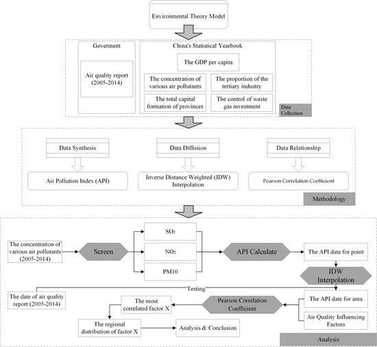
2.2. Basic Idea and Research Framework

• Environmental Theory Model [37]
The meaning of the environmental theory model is that environmental quality is affected by the per capita income, industrial structure and the adoption of environmental technologies. Each variable uses logarithms to characterize the nonlinear relationships with other variables and reduce the influence of heteroscedasticity. According to the environmental theory model, this article selects each index and air quality for the correlation analysis to obtain a strong index related to air quality for subsequent research.
• API Calculation
This article selected the API for the synthesis of air pollutant data to obtain comprehensive air quality data for data analysis. The Air Pollution Index (API) was used to evaluate the quality of the air in China from 2001–2012. The index synthesizes SO2, NO2 and PM10 information into a comprehensive value. After 2013, due to the heavy air pollution events, the Air Quality Index (AQCI) was adopted to replace the API in China. This index synthesizes information about SO2, NO2, PM10, PM2.5, CO and O3 [38]. In order to maintain the continuity of the data, this paper selected SO2, NO2 and PM10 from the air pollutant data in 2013 and 2014 for the API calculation and obtained API data for 2005–2014.
• Comparison of Inverse Distance Weighted Interpolation (IDW) and Kriging Interpolation Methods
IDW is a deterministic interpolation method which is estimated based on the weighted average [39]. The Kriging interpolation is also called the spatial local interpolation method. It can implement a linear optimal unbiased estimation of the data at unknown sampling points in a region [40]. IDW is more suitable for the proliferation of point source data, while Kriging is more suitable for continuous data diffusion. The monitoring point API data used in this paper are point source data and the air is fluid, so IDW was used for this study [41].
• Research Framework
The main flow of this paper was as follows: First, this paper selected the indicators under the environmental theory model for analysis and used the API calculation method to combine the air pollutant concentration data into API data, spatially interpolate the API data and use the interpolated data to carry out air pollution APIs in each province. The data were restatistically obtained by the provincial average API data, and finally, using the Pearson correlation analysis and the scatter plot curve fitting to analyze the relationship between air quality and the pollution treatment investment, the specific process was as shown Figure 2.

2.3. Data Collection

Table 1 shows the contents of the database used for this paper.
This paper included 310 data sets of five group from China’s Statistical Yearbook, comprising GDP per capita, concentration of various air pollutants, proportion of the tertiary industry, control of waste gas investment, and total capital formation of the provinces, which made it possible to reduce the impacts of spatial and temporal differences. The specific air quality monitoring sites are shown in Figure 1.

2.4. Methods

2.4.1. Environmental Theory Model

According to a previous literature review, the selection of environmental impact factors in this paper draws on the environmental theory model proposed by Dou [37], as shown in Equation (1):
E i t = β 0 + β 1 Y i t + β 2 S i t + β 3 T i t + μ i t
where E represents the environmental quality; Y represents per capita income (GDP per capita); S represents the industrial structure; T represents the adoption of environmental technologies; the subscripts i and t represent regions and years; and μ is the error term.

2.4.2. Air Pollution Index (API)

The Air Pollution Index (API) was used to evaluate the quality of air in China from 2001–2012. The index synthesizes SO2, NO2 and PM10 information into a comprehensive value, thus making it convenient for understanding [42]. The “China Statistical Yearbook” (2005–2012) only provides air contaminant concentration data of sulfur dioxide (SO2), nitrogen dioxide (NO2) and particulate matter (<10 μm) (PM10), and carbon monoxide (CO), ozone (O3) and particulate matter (<2.5 μm) (PM2.5) were added to air quality indicators after 2013. Out of consideration of data consistency, this paper used data on SO2, NO2 and PM10 from the years 2013 and 2014. The API calculation method used to process the data on SO2, NO2 and PM10 from 2005 to 2014 is shown in Equation (2) [42]:
A P I i = A P I U A P I L C U C L ( C i C L ) + A P I L
API = max   ( A P I i )
where A P I i is the index for pollutant i (i.e., PM10, SO2 and NO2); C i is the average concentration of pollutant i; C U and C L are the upper and lower breakpoints (the critical value of different pollutant levels) corresponding to C i , respectively; and A P I U and A P I L are the breakpoints of API corresponding to C U and C L , respectively. The overall API is the maximum A P I i (Table 2).

2.4.3. Inverse Distance Weighted (IDW) Interpolation

Considering that the point data from the monitor sites is incompatible with the realistic surface, and because air has a strong diffusion effect, inverse distance weighting (IDW [43]) was used to spread point-like data across the country. In this way, data on the surface air pollution of each province was obtained. By using IDW, it was possible to see air quality change from 2005 to 2014 more intuitively. The IDW formula was used to estimate the unknown factor of the monitoring station value, Z ( S 0 ) , in location S 0 , as shown in Equation (4) [44]:
Z ( S 0 ) = i = 1 n W i Z ( S i ) .
W i is the weight, defined as
W i = d o i α / i n d o i α
with
i n W i = 1
where n is the number of monitoring stations; d o i is the distance between the monitoring station and the unknown location; and α is an arbitrary positive real number.

2.4.4. Pearson Correlation Coefficient

The Pearson correlation analysis was used to analyze the API index versus the GDP per capita and the proportion of the tertiary industry in a given area to control the exhaust gas investment and to determine total capital formation. More relevant factors that influence air pollution were obtained from a follow-up analysis. The Pearson correlation coefficient ( r x ) for the five factors of each province-level city in China was calculated to assess their relationship [45]. r x was calculated with the p-value from the t-test, as shown in Equation (7):
r x = i = 1 n ( x i x ¯ ) i = 1 n ( x i x ¯ ) 2
where i ranges from 1 to 310 and represents the data group; n is the total number of data groups; x i is the statistics factor of group i ; x ¯ is the mean statistical factor of the groups. r x is regarded to be significantly different and credible when the p-value is below 0.05.

3. Results

3.1. Temporal and Spatial Changes in Air Quality in China

For a comparison of the air quality, we mapped the average air quality for the two five-year periods from 2005 to 2009 and 2010 to 2014 using raster calculator tools in ArcGIS (Figure 3).
The figure shows that the air pollution from 2005 to 2009 was aggravated, especially in Inner Mongolia (north of the map) and the north China region. The concentrated areas of air pollution from 2005 to 2009 included Northern Xinjiang (north-west of the map), Gansu (centre of the map), and Beijing (north-east of the map). In addition, from 2010 to 2014, atmospheric nitrogen (N) emissions increased by 38% due to industrial structure and transportation pressure [46], the air pollution situation in these three regions was aggravated, and due to the impact of dust storms and highly polluting industries [47] a new pollution concentration area emerged—Shaanxi (centre of the map). In addition, the pollution in Beijing shifted to the Southern part of Hebei (north-east of the map) where the pollution significantly increased. The air quality in Inner Mongolia was seriously affected by the north China region, and the air quality in south China also declined to some extent.
In order to assess the changes in air quality in more detail, the IDW was used to map China’s API interpolation from 2005 to 2014, as shown in the map in Figure A1.
During the period from 2005 to 2012, China’s general air quality stayed moderate. The pollution was mainly concentrated in Northern Xinjiang and Gansu, and the air quality in the monsoon region was relatively good. As the winter monsoon weakened in 2013, the weak wind speed, the longer duration of inversion across the country [5] and the long-term accumulation of pollution emissions, caused the air quality in the north China region to deteriorate, affecting air quality in most areas in Northern China. Furthermore, Southern provinces were also influenced, and the country’s overall air quality declined. Despite the air quality improvement in 2014, the situation of air pollution is far from optimistic.
In order to test the accuracy of the 34 sets of data, based on the monthly air quality report (Ministry of Ecology and Environment of the People’s Republic of China), this paper used 74 monitoring sites to perform IDW interpolating operations on the data from years 2013 and 2014 and acquired the composite air quality index (Figure 4) and determined the Pearson correlation coefficients of the correlation analysis between the API and AQCI data in ArcGIS (Table 3).
Through a comparison, it was found that the interpolation graph used in this study had a high degree of reliability, with the coefficient of correlation being between 0.942 and 0.917.

3.2. Temporal and Spatial Changes in Air Pollution Control Investment in China

To facilitate a comparison analysis, we mapped China’s air pollution control investment from 2005 to 2014 in Figure A2.
From 2005 to 2010, the air pollution investment was high in north China and Inner Mongolia, and was low in Northern Xinjiang, because the air quality in Northern Xinjiang is mainly affected by natural elements (high-frequency dust weather) [48]. From 2013, the nationwide investment on air pollution control increased significantly, which increased by 144% compared with 2012. China’s air quality showed a notable improvement in 2014, after the investment massively increased nationwide in 2013. Obviously, there was a lag in China’s air pollution control.

3.3. China’s Average Air Pollution Index (API) and Average Air Pollution Control Investment

In order to study the relationship between air pollution and the control investment, we drew a line graph of China’s yearly average API and yearly average control investment from 2005 to 2014 (Figure 5).
The line graph shows that China’s average API is in line with the trend of the average control investment in 2013. China experienced a wide range of serious air pollution incidents, and China’s investment in air pollution control has increased substantially. This also reflects the government’s emphasis on air pollution incidents. For instance, in 2013, China increased its investment in air pollution control after a wide range of air pollution incidents occurred in the same year, reflecting that the Chinese government was taking measures with high efficiency. However, this example also reveals the lagging effect of air control investment on air pollution, because the air quality appeared to improve about a year later. Figure 6 shows that with the growth in air pollution control investment, the correlation between investment control and air pollution changed from positive to negative, which is in line with the inverted ‘U’ line of the environmental Kuznets curve. This confirms the successful application of the curve in the study of air pollution control investment and air pollution.
Based on the Environmental Theory Model, Pearson correlation coefficients was used to assess every province’s data from 2005 to 2014 for average API, GDP per capita, proportion of the tertiary industry, air pollution control investment and total capital formation (Table 4). The average annual API of each province was obtained on the basis of Figure A1 using regional statistics.
The coefficient of correlation of 0.466 in the table indicates a significant positive correlation between China’s API value and air pollution control: the lower air quality in China, the higher investment put in air pollution control. Given the time series analysis and the spatial-temporal analysis in the above, it is not difficult to find that ‘Treatment after Pollution’ remains in terms of China’s economy. Pearson correlation coefficients highlight that ‘Treatment after Pollution’ did not work effectively for air quality improvement. The Chinese government needs to switch gears and accelerate industrial structure adjustment, so air pollution control in China should be transformed to accelerate the adjustment of industrial structure [49,50]. In summary, through the line graph and the curve graph, this paper reflects the existence of an inverted U-shaped relationship, similar to the environmental Kuznets curve, between the air pollution and control investment, namely, air pollution changing from positive to negative. According to the Pearson correlation analysis, China is still in a ‘Treatment after Pollution’ period, and it is in the transition period. Therefore, we suggest that China should continue to adjust its current industrial structure and increase its investment in pollution control in areas such as Shaanxi, Beijing, Hebei and Gansu to achieve point source governance, thus promoting surface source governance.

4. Discussion

4.1. Variable Selection and Applicability of the Environmental Kuznets Curve

The environmental Kuznets curve shows that environmental status and level of per capita income have an inverted U-shaped relationship. The capital in environmental Kuznets curve can be divided into two parts: one for production and spoiling the environment; the other for pollution control and improving the quality of the environment [51]. The pollution control part is similar to environment control investment. So, the environmental Kuznets curve is helpful in the study of air pollution and control investment.
The environmental Kuznets curve’s variable on the study of air environment is income and economic aggregate [52,53,54,55,56]. For instance, Selden et al. [53] used a cross-national panel of data on emissions of four important air pollutants: suspended particulate matter, sulfur dioxide, oxides of nitrogen, and carbon monoxide, and they found that the per capita emissions of all four pollutants exhibit inverted-U relationships with per capita GDP. Orub et al. [54] proved the existence of an environmental Kuznets curve for air suspended particulate matter through the study of the relationship between per capita income and environmental degradation in Africa. When the per capita income and per capita GDP are variable, under the same conditions of income, there are discrepancies in the control investment in different regions. So, taking the per capita income and per capita GDP as variables, there might be errors.
This paper used Kuznets curve as a reference and extended its scope of application. Instead of using per capita income and per capita GDP, we adopted air pollution control investment as a variable for accuracy. In this way, we were able to see the relationship between pollution control and ecological benefit. In addition, by analyzing the inflection point of the inverted U-shaped curve, we were able to answer the following question: what is the threshold number of control investment that improves air quality? However, a defect may still exist due to the fact that this curve is solely based on data covering the period from 2005 to 2014.

4.2. Limitations

Due to limited resources and data availability, we acknowledge the following limitations. Firstly, in terms of data precision, after 2013, two new indexes were added to China’s air quality monitoring indicators, PM2.5 and ozone (O3), which were not included in this study to allow data continuity. In addition, we only used 34 monitoring sets points, so the interpolation data accuracy still needs to be further improved. For the accuracy problem, this study used 34 sets of API interpolation maps and 74 site interpolation maps from 2013 and 2014 for the correlation analysis and obtained a high level of correlation. It is concluded that the data accuracy of this paper is good.
Secondly, the effect of interference factors presented a limitation. This paper mainly focused on the air pollution control status study in the secondary industry. Apart from industrial air pollution, less ink was given to other sources of air pollution. Still, this paper did not exclude the interference of other pollution sources with air quality. Future research will study how to analyze the status of multi-source air pollution control and investigate how to reduce the interference of irrelevant variables in the analysis.

5. Conclusions

Despite rapid economic growth, China’s air quality is still lower than developed countries. The air quality and control investment from 2005 to 2014 on a province-wide scale by IDW was analyzed by Pearson correlation. This paper concludes that (1) at present, there is a significant positive correlation between China’s API value and air pollution control with the coefficient of correlation being 0.466 (p-value < 0.01)—the lower air quality in China, the higher the investment put into air pollution control. ‘Treatment after Pollution’ remains a remarkable feature of China’s economy; (2) there is an inverted U-shaped relationship between China’s air pollution and control investment (2005–2014) which approximates the environmental Kuznets curve. In other words, an inflection point exists. Before the inflection point, there is positive correlation between air pollution and control investment. When the inflection point appears in the year of 2013 with the control investment of 2 billion yuan, the correlation turns negative; (3) Air pollution in north China is more serious than that in south China, and the distribution is consistent with the distribution of pollution control investment.
Deficiencies and further study directions in this paper are as follows: (1) This paper selected the air pollutant concentration data from 2005 to 2014. However, after 2013, the air quality monitoring index changed and new indicators were added. We used the API to allow good continuity; (2) this paper was limited by data in terms of studying the current status of air pollution control. It mainly focused on the study of the status of industrial air pollution control and dealt little with the control status of other pollution sources; (3) this paper did not establish an effective study system for air pollution control status due to limitations caused by data and technique. However, this study offers a new perspective into the study of air pollution in China and contributes to the literature on pollution control. Further study will be based on environmental pollution models, such as establishing a relationship model between air pollution and control investment, and the proportional hazards model (COX model) could also be used to conduct an air pollution risk assessment and establish an assessment model for air pollution and human health risk.

Author Contributions

P.S. conceived the entire paper, analyzed the data and designed the experiments. D.L. provided technical support, polished the text and provided project support. C.Q. provided writing and editing support. D.L. provided technical support and polished the text.

Funding

Natural Science Foundation of Zhejiang Province, China (LQ18D010003).

Acknowledgments

This study was supported by the Natural Science Foundation of Zhejiang Province, China (LQ18D010003). The valuable comments and suggestions from the editor and three anonymous reviewers are also greatly appreciated.

Conflicts of Interest

The authors declare no conflict of interest.

Appendix A

Figure A1. China’s air pollution index (API) distribution from 2005 to 2014.
Sustainability 10 02181 g0a1
Figure A2. China’s waste gas control investment distribution from 2005 to 2014.
Sustainability 10 02181 g0a2

References

  1. Tharby, R. (Ed.) Catching Gasoline and Diesel Adulteration (English); South Asia Urban Air Quality Management Briefing Note; NO. 7; World Bank: Washington, DC, USA, 2002; Available online: http://documents.worldbank.org/curated/en/223591468164352248/Catching-gasoline-and-diesel-adulteration (accessed on 13 June 2018).
  2. Ackermann-Liebrich, U.; Leuenberger, P.; Schwartz, J.; Schindler, C.; Monn, C.; Bolognini, G.; Bongard, J.; Brändli, O.; Domenighetti, G.; Elsasser, S. Lung function and long term exposure to air pollutants in Switzerland. Study on air pollution and lung diseases in adults (sapaldia) team. Am. J. Respir. Crit. Care Med. 1997, 155, 122–129. [Google Scholar] [CrossRef] [PubMed]
  3. Jiang, L.; Bai, L. Spatio-temporal characteristics of urban air pollutions and their causal relationships: Evidence from Beijing and its neighboring cities. Sci. Rep. 2018, 8, 1279. [Google Scholar] [CrossRef] [PubMed] [Green Version]
  4. Dockery, D.W.; Pope, C.A.; Xu, X.; Spengler, J.D.; Ware, J.H.; Fay, M.E.; Ferris, B.G., Jr.; Speizer, F.E. An association between air pollution and mortality in six US cities. N. Engl. J. Med. 1993, 329, 1753–1759. [Google Scholar] [CrossRef] [PubMed]
  5. Zhang, R.H.; Li, Q.; Zhang, R.N. Meteorological conditions for the persistent severe fog and haze event over eastern China in January 2013. Sci. China Earth Sci. 2014, 57, 10. [Google Scholar]
  6. Ma, J.; Zhang, W.; Luo, L.; Xu, Y.; Xie, H.; Xu, X. (Eds.) China Statistical Yearbook 2013; National Bureau of Statistics of People’s Republic of China, China Statistics Press: Beijing, China, 2013; Available online: http://www.stats.gov.cn/tjsj/ndsj/2013/indexch.htm (accessed on 13 June 2018). (In Chinese)
  7. Ashbaugh, L.L. A statistical trajectory technique for determining air pollution source regions. J. Air Pollut. Control Assoc. 1983, 33, 1096–1098. [Google Scholar] [CrossRef]
  8. Azimi, M.; Feng, F.; Yang, Y. Air pollution inequality and its sources in SO2 and NOx emissions among Chinese provinces from 2006 to 2015. Sustainability 2018, 10, 367. [Google Scholar] [CrossRef]
  9. Qiu, L.; He, L. Are Chinese green transport policies effective? A new perspective from direct pollution rebound effect, and empirical evidence from the road transport sector. Sustainability 2017, 9, 429. [Google Scholar] [CrossRef]
  10. Zhang, X.; Wang, Y.; Niu, T.; Zhang, X.; Gong, S.; Zhang, Y.; Sun, J. Atmospheric aerosol compositions in China: Spatial/temporal variability, chemical signature, regional haze distribution and comparisons with global aerosols. Atmos. Chem. Phys. 2012, 12, 779–799. [Google Scholar] [CrossRef] [Green Version]
  11. Li, R.; Cui, L.; Li, J.; Zhao, A.; Fu, H.; Wu, Y.; Zhang, L.; Kong, L.; Chen, J. Spatial and temporal variation of particulate matter and gaseous pollutants in China during 2014–2016. Atmos. Environ. 2017, 161, 235–246. [Google Scholar] [CrossRef]
  12. Zhao, H.; Ma, W.; Dong, H.; Jiang, P. Analysis of co-effects on air pollutants and CO2 emissions generated by end-of-pipe measures of pollution control in China’s coal-fired power plants. Sustainability 2017, 9, 499. [Google Scholar] [CrossRef]
  13. Xie, R.; Zhao, G.; Zhu, B.Z.; Chevallier, J. Examining the factors affecting air pollution emission growth in China. Environ. Model. Assess. 2018, 1–12. [Google Scholar] [CrossRef]
  14. Cong, X. Air pollution from industrial waste gas emissions is associated with cancer incidences in Shanghai, China. Environ. Sci. Pollut. Res. 2018, 25, 1–12. [Google Scholar] [CrossRef] [PubMed]
  15. Kuo, C.; Pan, R.-H.; Chan, C.-K.; Wu, C.-Y.; Phan, D.-V.; Chan, C.-L. Application of a time-stratified case-crossover design to explore the effects of air pollution and season on childhood asthma hospitalization in cities of differing urban patterns: Big data analytics of government open data. Int. J. Environ. Res. Public Health 2018, 15, 647. [Google Scholar] [CrossRef] [PubMed]
  16. Wang, M.; Zheng, S.; Nie, Y.; Weng, J.; Cheng, N.; Hu, X.; Ren, X.; Pei, H.; Bai, Y. Association between short-term exposure to air pollution and dyslipidemias among type 2 diabetic patients in northwest China: A population-based study. Int. J. Environ. Res. Public Health 2018, 15, 631. [Google Scholar] [CrossRef] [PubMed]
  17. Martinez, G.S.; Spadaro, J.V.; Chapizanis, D.; Kendrovski, V.; Kochubovski, M.; Mudu, P. Health impacts and economic costs of air pollution in the metropolitan area of skopje. Int. J. Environ. Res. Public Health 2018, 15, 626. [Google Scholar] [CrossRef] [PubMed]
  18. Cui, L.; Liu, X.; Geng, X.; Zhou, J.; Li, T. Effects of PM2.5 and haze event on hospital visiting of children in Ji’nan, 2013: A time series analysis. J. Environ. Health 2014, 6, 6. [Google Scholar]
  19. Zhang, J.; Liu, X. Influence of a severe dust storm on Chinese cities air quality. J. Desert Res. 2008, 28, 9. [Google Scholar]
  20. Ren, Y.; Shi, J.; Zhu, B.; Zhou, T. An analysis of weather condition during a continuous air pollution process in Nanjing city. Environ. Monit. Forewarn. 2012, 1, 004. [Google Scholar]
  21. Hu, J.; Wang, Y.; Ying, Q.; Zhang, H. Spatial and temporal variability of PM2.5 and PM10 over the North China plain and the Yangtze river delta, China. Atmos. Environ. 2014, 95, 598–609. [Google Scholar] [CrossRef]
  22. Zhang, Y.; Liu, Z.; Lv, X.; Zhang, Y.; Qian, J. Characteristics of the transport of a typical pollution event in the Cengdu area based on remote sensing data and numerical simulations. Atmosphere 2016, 7, 127. [Google Scholar] [CrossRef]
  23. Wang, L.K.; Pereira, N.C.; Hung, Y.-T. Air Pollution Control Engineering; Springer: New York, NJ, USA, 2004; Volume 1. [Google Scholar] [CrossRef]
  24. Zundel, T.; Rentz, O.; Dorn, R.; Jattke, A.; Wietschel, M. Control techniques and strategies for regional air pollution control from energy and industrial sectors. Water Air Soil Pollut. 1995, 85, 213–224. [Google Scholar] [CrossRef]
  25. Lakhani, H. Air pollution control by economic incentives in the US Policy, problems, and progress. Environ. Manag. 1982, 6, 9–20. [Google Scholar] [CrossRef]
  26. Hao, J.; He, K.; Duan, L.; Li, J.; Wang, L. Air pollution and its control in China. Front. Environ. Sci. Eng. China 2007, 1, 129–142. [Google Scholar] [CrossRef]
  27. Zhang, L.; Chen, C.; Murlis, J. Study on winter air pollution control in Lanzhou, China. Water Air Soil Pollut. 2001, 127, 351–372. [Google Scholar] [CrossRef]
  28. Feldstein, M. A new modeling technique for air pollution control. Environ. Manag. 1977, 1, 147–157. [Google Scholar] [CrossRef]
  29. Borghi, F.; Spinazzè, A.; Rovelli, S.; Campagnolo, D.; Del Buono, L.; Cattaneo, A.; Cavallo, D.M. Miniaturized monitors for assessment of exposure to air pollutants: A review. Int. J. Environ. Res. Public Health 2017, 14, 909. [Google Scholar] [CrossRef] [PubMed]
  30. Xia, Q.W.R. Discussion on the influencing factors of the investment effect of air pollution control in China based on the logarithmic mean diels’ decomposition method. Environ. Pollut. Control 2012, 34, 84–87. [Google Scholar]
  31. Tisdell, C. Globalisation and sustainability: Environmental Kuznets curve and the WTO. Ecol. Econ. 2001, 39, 185–196. [Google Scholar] [CrossRef]
  32. Grossman, G.M.; Krueger, A.B. Environmental Impacts of a North American Free Trade Agreement; National Bureau of Economic Research: Cambridge, MA, USA, 1991; Available online: http://www.nber.org/papers/w3914 (accessed on 13 June 2018).
  33. Xiao, K.; Wang, Y.; Wu, G.; Fu, B.; Zhu, Y. Spatiotemporal characteristics of air pollutants (PM10, PM2.5, SO2, NO2, O3, and CO) in the inland basin city of Chengdu, southwest China. Atmosphere 2018, 9, 74. [Google Scholar] [CrossRef]
  34. Wang, Z.; Ding, Y.; He, J.; Yu, J. An updating analysis of the climate change in China in recent 50 years. Acta Meteorol. Sin. 2004, 62, 228–236. [Google Scholar]
  35. Holzworth, G.C. (Ed.) Mixing Heights, Wind Speeds, and Potential for Urban Air Pollution throughout the Contiguous United States; Epa Publication, EPA: Washington, DC, USA, 1972; Available online: http://bases.bireme.br/cgi-bin/wxislind.exe/iah/online/?IsisScript=iah/iah.xis&src=google&base=REPIDISCA&lang=p&nextAction=lnk&exprSearch=163123&indexSearch=ID (accessed on 13 June 2018).
  36. Carslaw, D.C.; Ropkins, K. Openair—An r package for air quality data analysis. Environ. Model. Softw. 2012, 27, 52–61. [Google Scholar] [CrossRef]
  37. Dou, C. Economic Analysis of the Health Effects of Air Pollution. Southwest. Univ. Finance Econ. 2012. Available online: http://kns.cnki.net/KCMS/detail/detail.aspx?dbcode=CDFD&dbname=CDFD1214&filename=1012509650.nh&uid=WEEvREcwSlJHSldRa1FhdXNXa0hIUUVQY0t2bElUUXNqQkhNaExMMmJRRT0=$9A4hF_YAuvQ5obgVAqNKPCYcEjKensW4ggI8Fm4gTkoUKaID8j8gFw!!&v=MDAwNTNDamxXcjNJVkYyNkhMYTRGOWZKcjVFYlBJUjhlWDFMdXhZUzdEaDFUM3FUcldNMUZyQ1VSTEtmWWVScUY= (accessed on 13 June 2018). (In Chinese).
  38. Li, G.; Zhai, Q.; Huan, R.; Zhao, Y.; Liu, H.; Wu, H.; Zhuang, G. Monthly Air Quality Report 2013; Ministry of Ecology and Environment of the People’s Republic of China: Beijing, China, 2013. Available online: http://www.zhb.gov.cn/hjzl/dqhj/cskqzlzkyb/index_3.shtml (accessed on 13 June 2018).
  39. Shepard, D. A Two-Dimensional Interpolation Function for Irregularly-Spaced Data. In Proceedings of the 1968 23rd ACM National Conference, Las Vegas, NV, USA, 27–29 August 1968; ACM: New York, NY, USA, 1968; pp. 517–524. [Google Scholar]
  40. Kethireddy, S.R.; Tchounwou, P.B.; Ahmad, H.A.; Yerramilli, A.; Young, J.H. Geospatial interpolation and mapping of tropospheric ozone pollution using geostatistics. Int. J. Environ. Res. Public Health 2014, 11, 983–1000. [Google Scholar] [CrossRef] [PubMed]
  41. Qiao, P.; Lei, M.; Yang, S.; Yang, J.; Guo, G.; Zhou, X. Comparing ordinary kriging and inverse distance weighting for soil as pollution in Beijing. Environ. Sci. Pollut. Res. 2018, 25, 15597–15608. [Google Scholar] [CrossRef] [PubMed]
  42. Bao, J.; Yang, X.; Zhao, Z.; Wang, Z.; Yu, C.; Li, X. The spatial-temporal characteristics of air pollution in China from 2001–2014. Int. J. Environ. Res. Public Health 2015, 12, 15875–15887. [Google Scholar] [CrossRef] [PubMed]
  43. Anselin, L.; Le Gallo, J. Interpolation of air quality measures in hedonic house price models: Spatial aspects. Spat. Econ. Anal. 2006, 1, 31–52. [Google Scholar] [CrossRef]
  44. Madhloom, H.M.; Al-Ansari, N.; Laue, J.; Chabuk, A. Modeling spatial distribution of some contamination within the lower reaches of diyala river using idw interpolation. Sustainability 2017, 10, 22. [Google Scholar] [CrossRef]
  45. Chen, L.; Ren, C.; Zhang, B.; Wang, Z.; Liu, M. Quantifying urban land sprawl and its driving forces in northeast China from 1990 to 2015. Sustainability 2018, 10, 188. [Google Scholar] [CrossRef]
  46. Liu, X.; Xu, W.; Duan, L.; Du, E.; Pan, Y.; Lu, X.; Zhang, L.; Wu, Z.; Wang, X.; Zhang, Y. Atmospheric nitrogen emission, deposition, and air quality impacts in China: An overview. Curr. Pollut. Rep. 2017, 3, 65–77. [Google Scholar] [CrossRef]
  47. Zhang, X.; Gong, Z. Spatiotemporal characteristics of urban air quality in China and geographic detection of their determinants. J. Geogr. Sci. 2018, 28, 563–578. [Google Scholar] [CrossRef]
  48. Yang, X. An Analysis and Research of Present Atmospheric Environment in Northwest Region (Gansu, Qinghai, Xinjiang). Lanzhou Univ. 2012. Available online: http://kns.cnki.net/KCMS/detail/detail.aspx?dbcode=CMFD&dbname=CMFD201402&filename=1014301838.nh&uid=WEEvREcwSlJHSldRa1FhdXNXa0hIUUVQY0t2bElUUXNqQkhNaExMMmJRRT0=$9A4hF_YAuvQ5obgVAqNKPCYcEjKensW4ggI8Fm4gTkoUKaID8j8gFw!!&v=MjE2MzkxRnJDVVJMS2ZZZVJxRkNqbVZMN0tWRjI2R3JDNEg5blBwNUViUElSOGVYMUx1eFlTN0RoMVQzcVRyV00= (accessed on 13 June 2018). (In Chinese).
  49. Chan, C.K.; Yao, X. Air pollution in mega cities in China. Atmos. Environ. 2008, 42, 1–42. [Google Scholar] [CrossRef]
  50. He, J. Pollution haven hypothesis and environmental impacts of foreign direct investment: The case of industrial emission of sulfur dioxide (SO2) in Chinese provinces. Ecol. Econ. 2006, 60, 228–245. [Google Scholar] [CrossRef]
  51. Dinda, S. Environmental Kuznets curve hypothesis: A survey. Ecol. Econ. 2004, 49, 431–455. [Google Scholar] [CrossRef] [Green Version]
  52. Torras, M.; Boyce, J.K. Income, inequality, and pollution: A reassessment of the environmental Kuznets curve. Ecol. Econ. 1998, 25, 147–160. [Google Scholar] [CrossRef]
  53. Selden, T.M.; Song, D. Environmental quality and development: Is there a Kuznets curve for air pollution emissions? J. Environ. Econ. Manag. 1994, 27, 147–162. [Google Scholar] [CrossRef]
  54. Orubu, C.O.; Omotor, D.G. Environmental quality and economic growth: Searching for environmental Kuznets curves for air and water pollutants in Africa. Energy Policy 2011, 39, 4178–4188. [Google Scholar] [CrossRef]
  55. Carson, R.T.; Jeon, Y.; McCubbin, D.R. The relationship between air pollution emissions and income: US data. Environ. Dev. Econ. 1997, 2, 433–450. [Google Scholar] [CrossRef]
  56. Stern, D.I. The rise and fall of the environmental Kuznets curve. World Dev. 2004, 32, 1419–1439. [Google Scholar] [CrossRef]
Figure 1. The location of the study area. Each point is an air quality monitoring station in China.
Sustainability 10 02181 g001
Figure 2. The outline of the study structure. (1) Based on a previous literature review, the selection of environmental impact factors in this paper drew on the Environmental Theory Model proposed by Dou [37]. (2) The data sources are listed in the first part of the figure. We chose data from “China’s Statistical Yearbook” for analysis and data from the Ministry of Ecology and Environment of the People’s Republic of China for verification. (3) The main methods in this paper are listed in the second part of the figure. We used API for data synthesis, IDW for data diffusion and the Pearson Correlation Coefficient for data relationships. (4) The analysis procedures are listed in the third part of the figure. We screened, combined and diffused data from “China’s Statistical Yearbook” for further analysis of the Pearson Correlation Coefficient and used the data from the Ministry of Ecology and Environment of the People’s Republic of China to test the accuracy of the air quality data.
Sustainability 10 02181 g002
Figure 3. Comparison of average air quality between 2005–2009 and 2010–2014.
Sustainability 10 02181 g003
Figure 4. China’s air quality composite index (AQCI) distribution in 2013 and 2014.
Sustainability 10 02181 g004
Figure 5. Provincial API and air pollution control investment line chart.
Sustainability 10 02181 g005
Figure 6. Provincial API and air pollution control inverted ‘U’ curve chart.
Sustainability 10 02181 g006
Table 1. Datasets for air pollution and changes in control investment.
Data NameData ContentTemporal ResolutionData Sources and URL
GDP (Gross Domestic Product) Per PersonPer capita GDP of provinces in China2005–2014China’s Statistical Yearbook, http://www.stats.gov.cn/tjsj/ndsj/
Air PollutantsChina’s annual data of sulfur dioxide (SO2), nitrogen dioxide (NO2) and fine particles (<10 μm) (PM10)2005–2014China’s Statistical Yearbook, http://www.stats.gov.cn/tjsj/ndsj/
Industry StructureProportion of the tertiary industry in China2005–2014China’s Statistical Yearbook, http://www.stats.gov.cn/tjsj/ndsj/
Control InvestmentInvestment completed for the treatment of waste gas which includes capital investment in the industrial air pollution sources and urban air governance infrastructure.2005–2014China’s Statistical Yearbook, http://www.stats.gov.cn/tjsj/ndsj/
Total Capital FormationTotal capital formation of each province in China2005–2014China’s Statistical Yearbook, http://www.stats.gov.cn/tjsj/ndsj/
Air Quality Composite IndexAir quality composite index for China for each month.2013,2014The Ministry of Ecology and Environment of the People’s Republic of China, http://www.mep.gov.cn
Note: In total, 304 sets of data were used, except for the air quality composite index which had 74 sets of data.
Table 2. The concentration breakpoints for each pollutant in the calculation of the API.
Pollutant Concentrations (μg/m3)API
PM10SO2NO2
0000
150150120100
350800280200
4201600565300
5002100750400
6002620940500
Table 3. The Pearson correlation coefficient of the correlation analysis between API and AQCI data.
Group Name r x
API (34sites) & AQCI (74sites) in 20130.942 **
API (34sites) & AQCI (74sites) in 20140.917 **
Note: ** denotes strongly significant with a p-value below 0.01.
Table 4. The Pearson correlation coefficients of the correlation analysis between API and statistical data.
Statistical Data Related to API r x
The GDP per capita (yuan)0.165 **
The proportion of the tertiary industry (%)−0.096
The air pollution control investment (ten thousand yuan)0.466 **
The total capital formation (ten million yuan)0.230 **
Note: Due to the lack of data on the air pollution control investment in Tibet during the period from 2005–2010, the sample size is 304. The spatial scale of the data is province-wide, and temporal scale of the data is from 2005 to 2014. ** denotes strongly significant with a p-value below 0.01.

