Article

Hybrid Forecasting Model for Short-Term Electricity Market Prices with Renewable Integration

by
Gerardo J. Osório
1,
Mohamed Lotfi
2,3,
Miadreza Shafie-khah
2,
Vasco M. A. Campos
3 and
João P. S. Catalão
2,3,*
1
Center for Mechanical and Aerospace Science and Technologies, University of Beira Interior, 6201-001 Covilhã, Portugal
2
INESC TEC, 4200-465 Porto, Portugal
3
Faculty of Engineering, University of Porto, 4200-465 Porto, Portugal
*
Author to whom correspondence should be addressed.
Submission received: 21 November 2018 / Revised: 17 December 2018 / Accepted: 18 December 2018 / Published: 22 December 2018
(This article belongs to the Special Issue Wind Energy, Load and Price Forecasting towards Sustainability 2019)

Abstract

:
In recent years, there have been notable commitments and obligations by the electricity sector for more sustainable generation and delivery processes to reduce the environmental footprint. However, there is still a long way to go to achieve necessary sustainability goals while ensuring standards of robustness and the quality of power grids. One of the main challenges hindering this progress are uncertainties and stochasticity associated with the electricity sector and especially renewable generation. In this paradigm shift, forecasting tools are indispensable, and their utilization can significantly improve system operation and minimize costs associated with all related activities. Thus, forecasting tools have an essential key role in all decision-making stages. In this work, a hybrid probabilistic forecasting model (HPFM) was developed for short-term electricity market prices (EMP) combining wavelet transforms (WT), hybrid particle swarm optimization (DEEPSO), adaptive neuro-fuzzy inference system (ANFIS), and Monte Carlo simulation (MCS). The proposed hybrid probabilistic forecasting model (HPFM) was tested and validated with real data from the Spanish and Pennsylvania-New Jersey-Maryland (PJM) markets. The proposed model exhibited favorable results and performance in comparison with previously published work considering electricity market prices (EMP) data, which is notable.

1. Introduction

In competitive and liberalized markets with prominent renewable integration, the natural renewable stochasticity is echoed in all market players’ decisions, bringing additional challenges in the way of achieving a sustainable, profitable, and reliable operation of the electricity structure [1]. Moreover, the microgeneration together with the natural evolution of renewable energy technologies is leading to a paradigm shift of the electricity sector [2].
This, in addition to other factors, often make electricity market prices (EMP) forecasting tools more vital than demand series forecasting tools [3]. A way to increase the sector flexibility is by integrating innovative storage systems, where the main goal is to manage the unpredictable behavior of renewables. However, this is highly costly, the lifetime is limited, and in most of the cases, prototypal systems are used [4,5,6].
Therefore, the study of forecasting EMP has grown as one of the biggest research areas [7]. EMP forecasting is a critical and inevitable task for all agents participating in different electricity market activities, and, moreover, in the presence of smart grid and smart house concepts [8].
This is especially the case with the advance of smart grids, the aforementioned paradigm shift in the electricity sector, and the necessary and unavoidable mitigation of the human footprint impact due to climate change and other environmental concerns [9].
The scientific literature shows that several techniques for EMP forecasting models are categorized [10] into different time horizons: (1) Very-short-term (few seconds to few hours), (2) short-term (few hours to few days), and (3) long-term (few days to few months) [11].
In the case of hard computing, the most known models are related with the auto-regressive integrated moving average (ARIMA), with or without data pre-processing [12], where a huge amount of physical data is needed and an exact modelling of the structure is mandatory.
In contrast, soft computing models generally use an auto-learning procedure from historical information to recognize expected data with outlines present in the historical data. A wide range of models exist, mostly associated with artificial neural network (NN) philosophy, such as [13,14], and hybrid models [15,16,17,18], where the objective is to exploit the best features from the sets’ techniques that compose the forecasting model.
Nowadays, the efforts of the scientific community are focused on innovative probabilistic forecasting models, where the hybridization of different methods is common, but with the goal of more realistic and spread outputs [19,20,21,22]. To validate the accuracy and applicability of proposed forecasting models, the usage of similar historical datasets is necessary, not with the goal of tuning the model, but to prove its advantages among other proposed models.
For example, in Reference [23], a hybrid forecasting model was presented and applied to forecast different time horizons (i.e., for the next day- and week-ahead EMP), considering different sets of historical data from two electricity markets commonly used to validate forecasting models.
In Reference [9], a hybrid forecasting model was presented, combining wavelet transforms (WT), hybrid particle swarm optimization (DEEPSO), and adaptive neuro-fuzzy inference system (ANFIS) methods to forecast the EMP series for the Spanish market (2002, 2006), and Pennsylvania-New Jersey-Maryland (PJM) markets (2006), with different forecasting windows (i.e., between 24 h and 168 h ahead) with a 1-h time-step. The model was validated by comparison with previous approaches considering the same real and historical data.
In Reference [14], a hybrid forecasting approach was presented considering a pre-processing technique combining particle swarm optimization (PSO) and fuzzy neural networks techniques to forecast and classify the EMP of the Spanish electricity market. In the same trend of research, in Reference [1], a forecasting model was proposed composed by the support vector network with an ANFIS network in order to analyze the information of the Nordpool power market in Denmark.
In Reference [24] a hybrid approach was proposed for market clearing prices considering forecasting intervals and point forecast through a modified dolphin echolocation optimization algorithm combined with WT and NN. Uncertainties and noise variance were considered. Real EMP data from Ontario, New England, and Australian electricity markets were used for validation.
Furthermore, in Reference [25], a probabilistic hybrid EMP forecasting EMP based on an improved clonal selection algorithm and extreme learning machine for NN and WT was proposed. An autocorrelation process was also used to reduce computational costs. Real EMP data from Ontario and Australian electricity markets were also used for validation.
Considering the widespread state-of-the-art tools and the importance of considering probabilistic tools for forecasting, in this work, a probabilistic hybrid forecasting model is elaborated and explored for short-term EMP. The proposed model uses a combination of WT, as a pre-processing data technique, with DEEPSO in order to reduce the overall forecasting error by tuning ANFIS parameters. Afterwards, the resulting forecasted data is analyzed and post-processed using a Monte-Carlo simulation (MCS) model to extract the expected deviation from the forecasted results.
The proposed model is hereafter referred to as a hybrid probabilistic forecasting model (HPFM). The proposed HPFM was used to forecast the Spanish and PJM EMP, without exogenous data, considering the next week with a time-step of 1 h. The results were compared with other proposed models already published considering the same historical data and without relying on any external exogenous input data for the sake of a fair comparison.
The manuscript is ordered as follows: Section 2 describes the proposed hybrid model, explaining in detail the underlying concepts of the incorporated algorithms (WT, DEEPSO, ANFIS, and MCS). Section 3 shows the most commonly used forecasting validation tools and the ones used by this work to validate the proposed model. Section 4 presents the case studies and obtained results. Finally, in Section 5, the conclusions are provided.

2. Proposed Hybrid Probabilistic Forecasting Model (HPFM)

The proposed HPFM employs wavelet transforms (WT) to capture some features from the random behavior of electricity market prices (EMP). The hybrid particle swarm optimization (DEEPSO), due to the differential evolutionary process and hybrid enhancements, brings better capabilities to the ANFIS structure to reduce the forecast error through the tuning of ANFIS membership functions, providing a first-stage result. The resulting data is then analyzed through the Monte-Carlo simulation (MCS) model, where the goal is to have the capability of knowing the forecasted values’ range without increasing the forecast error.

2.1. Wavelet Transforms (WT)

In current forecasting models used for the analysis of time series, such as EMP and renewable power, WT has been widely used because it can detect patterns and trends without losing the original information. Both the above-mentioned time series exhibit intermittency, volatility, and peak trends that are challenging to forecast. In this sense, WT can be considered as a tool capable of isolating these trends from a non-stationary time series [19]. Moreover, WT was successfully used for power quality and transient analysis, modeling of short-term energy system disturbances, and other signal analyses in a continuous or discrete domain [18].
Mathematically, data processing of a time-varying input signal, x ( t ) , at multiple resolutions is done by scaling and translating a mother function, Ψ ( t ) , by a convolution integral, allowing the illustration of the time series in the time and frequency domains [19]. The scaling ( a ) and translating ( b ) factors are applied to the mother function, Ψ ( t ) , such that:
Ψ a , b ( t ) = 1 a ψ ( t b a ) ;   a > 0 ,   < b <
Using the complex conjugate, Ψ * , the continuous wavelet transform is obtained as follows [26]:
C W T x ( a , b ) = 1 a Ψ * ( t ) x ( t ) d t ;   a > 0  
By combining Equations (1) and (2), and discretizing, the more computationally efficient discrete WT (DWT) can be obtained and is expressed as:
D W T x ( m , n ) = 2 ( m / 2 ) × t = 0 T 1 x ( t ) × ψ ( t n × 2 m 2 m )
In this form: T is the sampled signal length, m and n are the DWT counterparts of scaling factors a and b such that m = log 2 ( a ) and n = log 2 ( b ) . In the method proposed by this work, DWT was used for: (1) Signal decomposition, and (2) signal reconstruction. This was done using a multiresolution analysis based on a three-level variation of Mallat’s algorithm, which allows a filter-based DWT implementation with an iterative process [27].
In the case of decomposition, the input signal ( t ) is divided into components of lower resolution, making up the WT decomposition tree. This signal at a first level is passed through a low-pass filter and a high-pass filter, and then the filter outputs are subtracted by 2, resulting in the first-level approximation and detail coefficients ( A 1 , and D 1 ). This is repeated until the desired levels are reached ( A n , and D n ). In a similar manner, the reconstruction process has three iterations of sampling followed by filtering, resulting in six coefficients, three of approximation and three of detail [26].

2.2. Hybrid Particle Swarm Optimization (DEEPSO)

Particle swarm optimization (PSO) is a stochastic, bio-inspired, population-based, swarm intelligence method developed by [28]. Being a swarm intelligence method, the algorithm mimics the social behavior and dynamics of swarming phenomenon in nature (e.g., bird flocks). In PSO, each particle in the population represents a potential solution to the objective function.
Each particle’s position vector within the multi-dimensional search space corresponds to values of solution variables (i.e., design vector). As the swarm “flies” through the search space, the objective function for each particle is calculated from its position vector.
At the end of every iteration, each particle trajectory, or velocity, is updated depending on: (1) Whether its objective function is increasing or decreasing (local knowledge), (2) the trajectories of neighboring particles (global knowledge), and (3) the best solution historically found by the swarm (global knowledge). The updating of individual trajectories happens iteratively based on the combined use of local, global, and historical knowledge, allowing the swarm to collectively “fly” towards more optimal solution points, ideally converging to the global optimum in the search space [29].
Evolutionary computing, the most famous of which are genetic algorithms (GA), is another class of stochastic, bio-inspired, population-based methods. Unlike PSO, they are driven by survival of the fittest rather than social behavior [30]. The population of potential solutions share global knowledge through the simulation of natural selection (Darwinism). The population “evolves” in every iteration through crossover of different individuals. The choice thereof is based on deterministic (fitness) and random factors. In addition, mutation operators allow random changes to occur to some individuals every iteration.
While GA is older than PSO, they have recently been less popular in comparison due to the fact they are more complex, with many parameters that need to be defined and re-tuned for different problems. PSO has been shown to outperform GA computationally in addition to being easier to implement due to its algorithmic simplicity with less parameters, despite having a static population set due to lacking operators, such as mutation and crossover (allowing a random element of information exchange between the population as opposed to deterministic trajectory updates), which can lead to the algorithm being stuck in local minima [31].
Evolutionary PSO (EPSO) is an enhanced version of PSO, which aims to incorporate the advantages of evolutionary computing. A control parameter of PSO is the weight, w , of particles, which provides damping of the trajectory updating. In EPSO, particle weights are subjected to a mutation operator, and the swarm is altered by evolutionary features in every iteration. The hybrid algorithm enhances the performance of PSO [32].
Differential EPSO (DEEPSO) takes this one step further, with the weight parameters, w i k * , having auto-adaptive properties. While EPSO subjects the weights to a mutation operator, DEEPSO incorporates a crossover operator (as in GA), generating a new solution for particles as a fraction of that of the two other particles [18]. As such, for every particle, i , in a swarm of a size, N , the individual trajectories are updated in each iteration, k , as follows:
  • Position:
    X i ( k ) = X i ( k 1 ) + V i ( k ) ;       i = 1 ,   2 ,   ,   N
  • Velocity:
    V i ( k ) = w i 0 * V i ( k 1 ) + w i 1 * ( X r 1 i ( k 1 ) X r 2 i ( k 1 ) ) + P w i 2 * ( G b e s t , i * X i ( k 1 ) )
X i ( k ) and X i ( k 1 ) are the new and previous positions of particle i (in iteration k ), respectively. X r i is any duo of different particles previously sampled from the swarm. G b e s t , i * is the best global position, selected based on a random Gaussian variable with a mean = 0 and variance = 1 ( N ( 0 , 1 ) ) . P is a diagonal binary matrix with a value of 1 when the probability is p and 0 when the probability is { 1 p } . Moreover, w i n * are the particle inertias (also the memory and cooperation weights), which are mutated each iteration through the learning mutation parameter, τ .
The differential evolutionary features added to PSO are:
  • Particle Weights Mutation:
    w i k * = w i k + τ N ( 0 , 1 ) ,
  • Current Best Position with Normal Distribution
    G b e s t , i * = G b e s t , i × ( 1 + w g N ( 0 , 1 ) ) ,   and
  • Differential Set for Particle Crossover:
    P = f ( X r 1 i ( k 1 ) ) < f ( X r 2 i ( k 1 ) )
The components, X r n i , guarantee that an appropriate extraction truly occurs, through the consideration of macro-gradient points in a descending way, depending on the organized comparison. Through this idea, the component, X r 2 i , is presumed to be X r 2 i = X i , and the component, X r 1 i , is selected from the set of the best ancestors of the swarm.

2.3. Adaptive Neuro-Fuzzy Inference System (ANFIS)

ANFIS is able to work with a large amount of data using a smaller computational requirement [15]. The structure of the ANFIS network is composed of five layers, where each layer contains nodes described by the node function, O i j . ANFIS is a hybrid model combining the best features of NN structures and fuzzy inference system (FIS) features. As demonstrated in the state-of-the-art review, ANFIS is capable of processing considerable lengths of data using low computational requirements. In addition, the ANFIS incorporates self-learning capabilities, which helps to self-adjust its parameters [18].
The combination of NNs with FIS takes advantage of the best of both: NN extracts fuzzy rules from the data automatically, while in the learning process, fuzzy logic is applied with the adjustment of membership functions. As stated before, the ANFIS model is composed of five layers: Fuzzification process, firing strength rules, normalization, defuzzification, and output; which are interconnected with the different inputs and resulting in one output. The forecast results in a Takagi-Sugeno structure [18,27].

2.4. Monte-Carlo Simulation (MCS)

MCS is a powerful instrument of analysis and has long been employed on engineering problems. MCS is typically used to model an intrinsic variable of a system in which analytical formulae cannot be used due to complexity [33]. An example of an MCS application can be found in [34], where the effects of renewable integration with the interruptions’ probability were studied; where not only the uncertainty of components failure was analyzed, but also the variability of renewable integration was considered.
In this work, MCS was employed to analyze the result of the forecast for a range of values where the forecast can be inserted. With this, it is possible to have a probabilistic forecast result for further realistic analyses and decision making. MCS with variable control was implemented, whose concept is described as computing the analysis results around which the obtained values do not diverge from the expected real values [35].
The historical dataset, X = ( x 1 , ,   x s ) , is experimented according to its probabilistic distributions. Afterwards, the forecast results set, Y , were computed through the performance function, Y = g ( X ) , containing input variables.
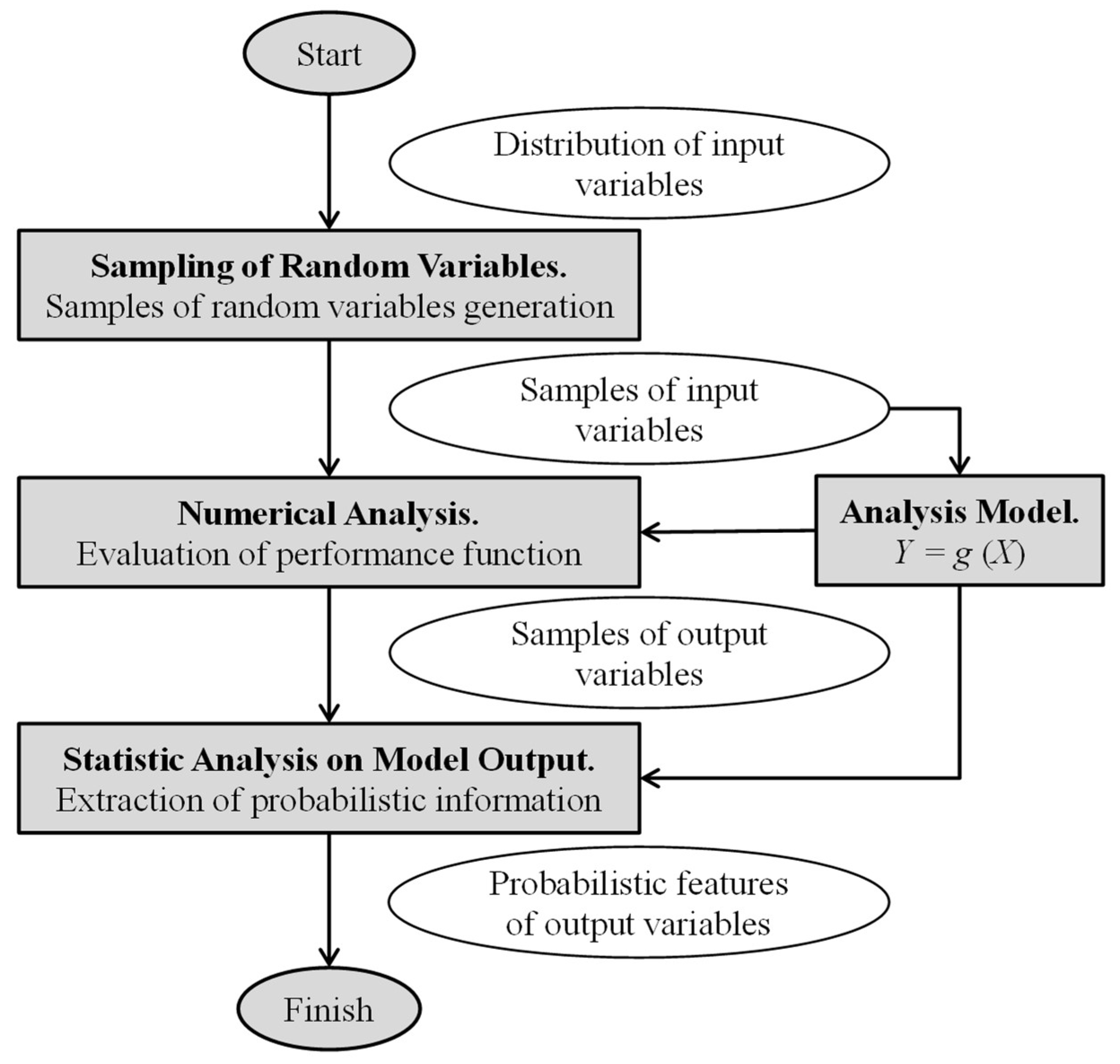
Afterwards, statistical features of the output variables, Y , were estimated. The basic structure of this model is shown in Figure 1. Supposing that a set of S samples of random variables are generated, it means that all generated samples constitute a set of inputs, x i = ( x i 1 , , x i S ) ,   i S , for the model, Y = g ( X ) , i.e., [35]:
y i = g ( x i ) ,   i = 1 , 2 , , S
After obtaining the output samples, a statistical study can be done to estimate the output features, Y , i.e., the mean, variance, reliability, probability of failure, the probability density function (PDF), and the cumulative density function (CDF). The meanings associated with these features are represented in the following equations:
  • The mean:
    Y ¯ = 1 S × i = 1 S y i
  • The variance:
    σ γ 2 = 1 S 1 × i = 1 S ( y i Y ¯ ) 2
  • The probability of failure expression in case of g 0 :
    p f = P { g 0 } p f = + I ( x ) f x ( x ) d x
    where:
    I ( x ) = { 1 ,                 i f     g ( x ) 0 0 ,                   i f   g ( x ) > 0
As the integral of the previous equation is only the average value of I ( x ) , the probability of failure is rewritten as:
p f = Y ¯ = 1 S × i = 1 S I ( x i ) = S f S
where S f is the total of samples that have a performance function lower or equal to 0. After this step, the cumulative density function is:
F y ( y ) = P ( g y ) = 1 S × i = 1 N I ( y i )
where the indicator function, I , is:
I ' ( x ) = { 1 ,                 i f     g ( x ) y 0 ,                   i f   g ( x ) > y
Finally, the PDF can be obtained from the numerical differentiation of CDF.

2.5. Probabilistic Hybrid Forecasting Model (PHFM)

The flowchart of the proposed PHFM is illustrated in Figure 2. In brief, the algorithm can be described in the following list of steps:
  • Step 1: Start the PHFM model with a historical data of EMP, taking as window frames the forecasting time-frame (168 h for each set chosen);
  • Step 2: Select the historical data that will be decomposed by the WT;
  • Step 3: Select the parameters of the DEEPSO (Table 1);
  • Step 4: Select the set of weeks that will be used in DEEPSO to obtain the necessary features to tuning and increase the performance of the ANFIS model;
  • Step 5: Select the parameters of the ANFIS (Table 1);
  • Step 6: Select the inputs of each iteration of the ANFIS method;
  • Step 7: Calculate the forecasting errors with the different error measurements criterions to authenticate the advances of the proposed PHFM model:
    Step 7.1: If the criterion error goal is not achieved, start Step 7 again;
    Step 7.2: If the criterion error goal is not found in Step 7, jump to Step 4 to find another set of solutions;
    Step 7.3: If the best forecasting results are found, or the number of the iteration is reached, save the latest best record and go to Step 8;
  • Step 8: Use the inverse of the WT transform to include the data previously filtered in the forecasted output;
  • Step 9: Obtain the analysis result using the MCS; print the forecasting results and finish.

3. Forecasting Validation

To analyze the forecasting EMP results obtained by the proposed PHFM algorithm with other available and published ones, which use the same input historic EMP sets, the mean absolute percentage error (MAPE) measure was used.
From MAPE, p ^ n s is the PHFM output at time n s ; p n s is the EMP data at time n s ; p ¯ is the EMP average result for the forecasting data; and N s is the dimension number of input data. From the similar definition resulted from MAPE, the uncertainty of the PHFM is computed considering the (weekly) error variance:
σ e , n s 2 = 1 N s × n = 1 N s ( | p ^ n s p n S | p ¯ e n s ) 2
e n s = 1 N s × n s = 1 N S | p ^ n s p n s | p ¯
It should be noted that the average EMP is used (for both electricity markets under analysis) for MAPE and error variance criteria to avoid numerical instability caused when prices tend to be zero [16].

4. Case Studies and Results

The proposed PHFM was tested using an input 6 weeks of historical data to provide forecast results for the next week-ahead with 1-h increments. Well-known real data from the Spanish EMP of the year, 2002, and from the PJM EMP for the winter season of 2006 were used More details are available about the datasets and can be found in Reference [18]. Moreover, in accordance with published and validated studies, no exogenous data was considered to achieve a fair and valid comparison between their results and this study. Implementation and execution of the model were on a common PC (Intel processor i3-2310, @2.10 GHz, 4 GB RAM) using MATLAB 2016b.
The average computation time to obtain a single forecasting result was around 1 min. 
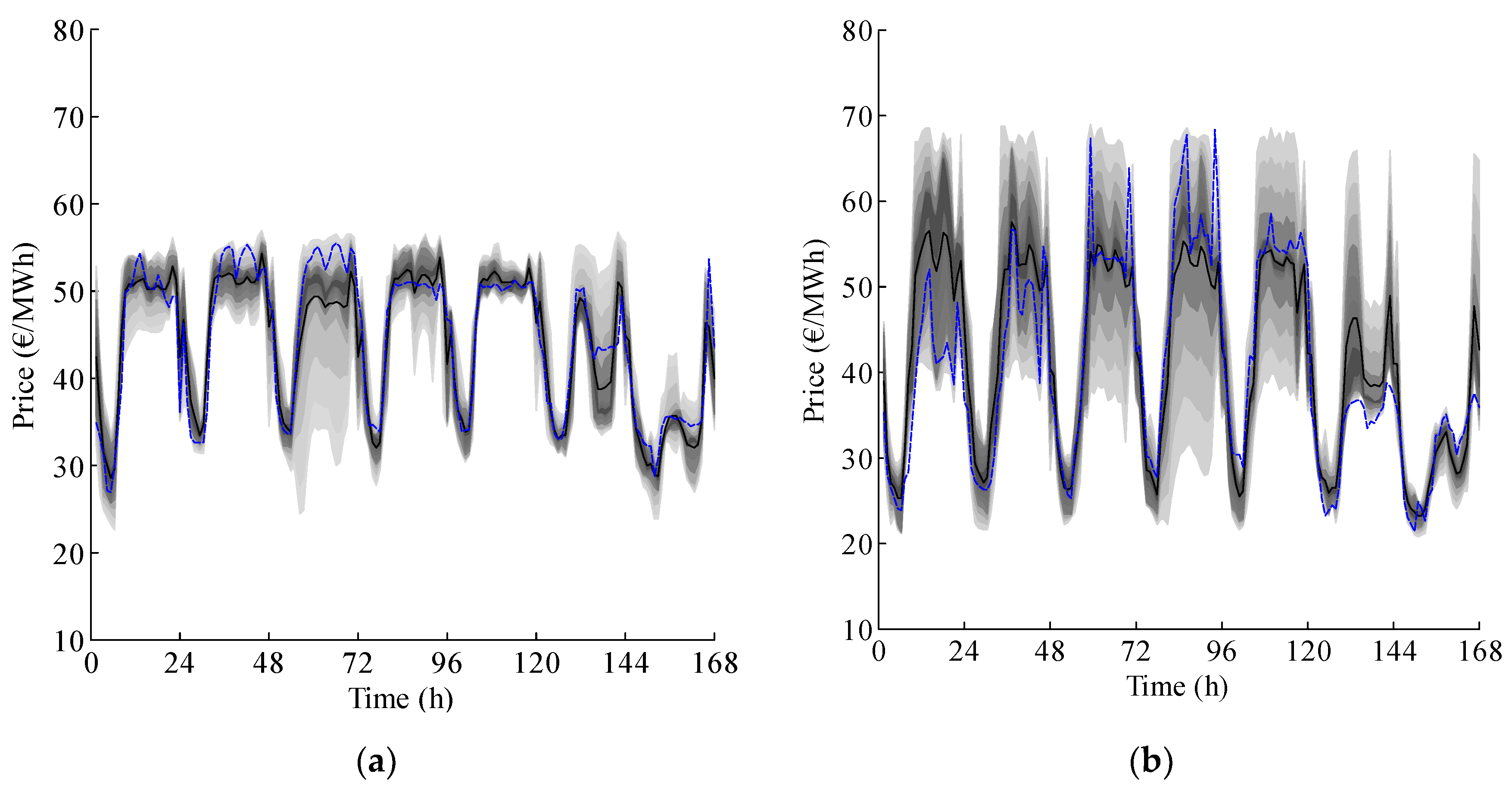
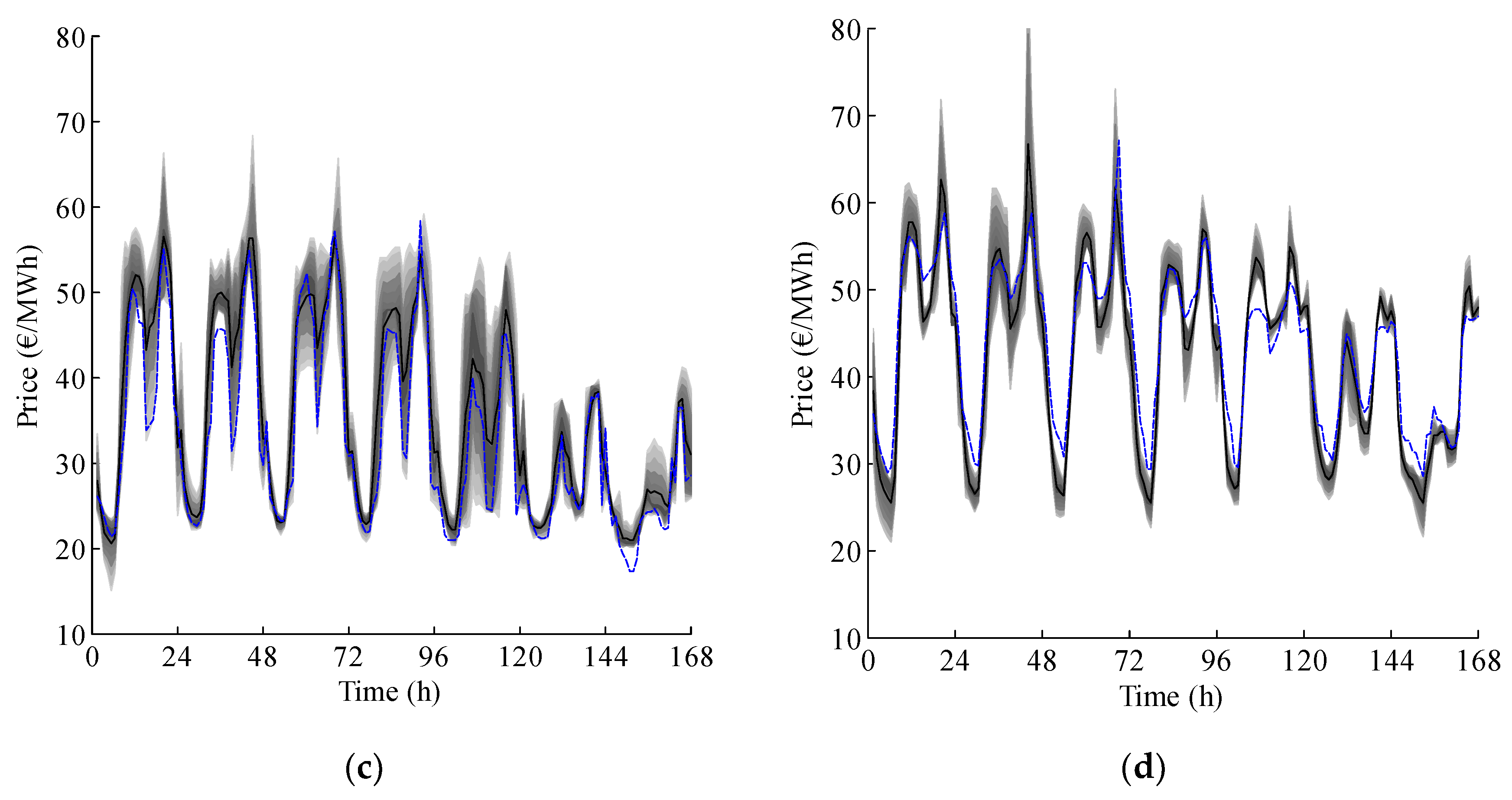
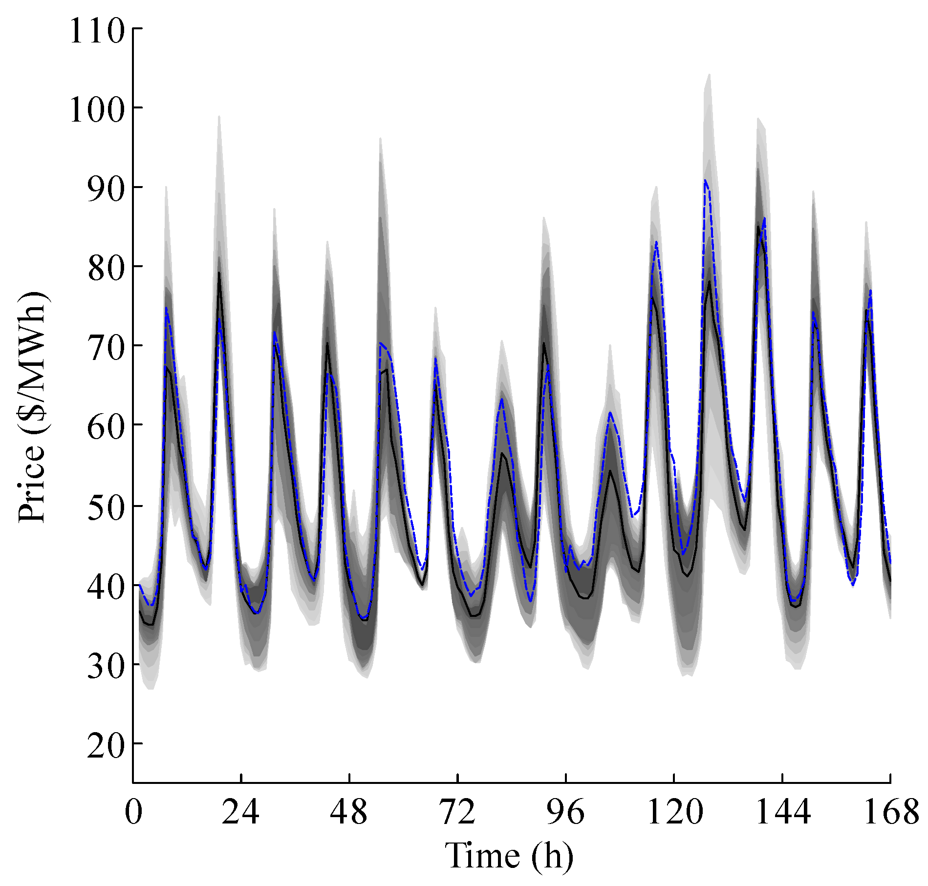
Figure 3 shows the numerical results for the different sample weeks of the year (spring, summer, fall, and winter) of the Spanish EMP, and Figure 4 for the week of 22–28 February of the PJM market.
From the numerical results obtained it is possible to observe how the PHFM model handled the uncertainty of markets and different seasons under analysis. Moreover, the precision of the forecasted values throughout the weeks under analysis was observed.
The MCS analysis allows the observation of how the forecasting values may fluctuate due to uncertainty and stochasticity incorporated inherently in the algorithms and historical data. In fact, the shaded areas in Figure 3a,b, which are produced by MCS, visualize that some days are associated with a higher uncertainty of the forecasting accuracy. Specifically, hour 48 to hour 72 in Figure 3a, shows that the proposed model may have more difficulties obtaining optimal results in this period due to the high uncertainty of the forecasting accuracy.
Moreover, in Figure 3b, an even higher range of uncertainty was encountered. This is mainly due to the price spikes behavior (a phenomenon which is out of scope for this study). However, despite the presence of high uncertainties and price spikes, the proposed forecasting model provides good results throughout those weeks.
Table 2, Table 3, Table 4 and Table 5 present the evaluation between PHFM with other previous hybrid models with intelligence features in the scientific community, regarding MAPE criterion, and weakly error variance criterion for the Spanish and PJM markets in each season. Table 5 outlines the performance of the proposed PHFM considering the mean, variance, and maximum and minimum error corresponding to all test cases. Finally, 
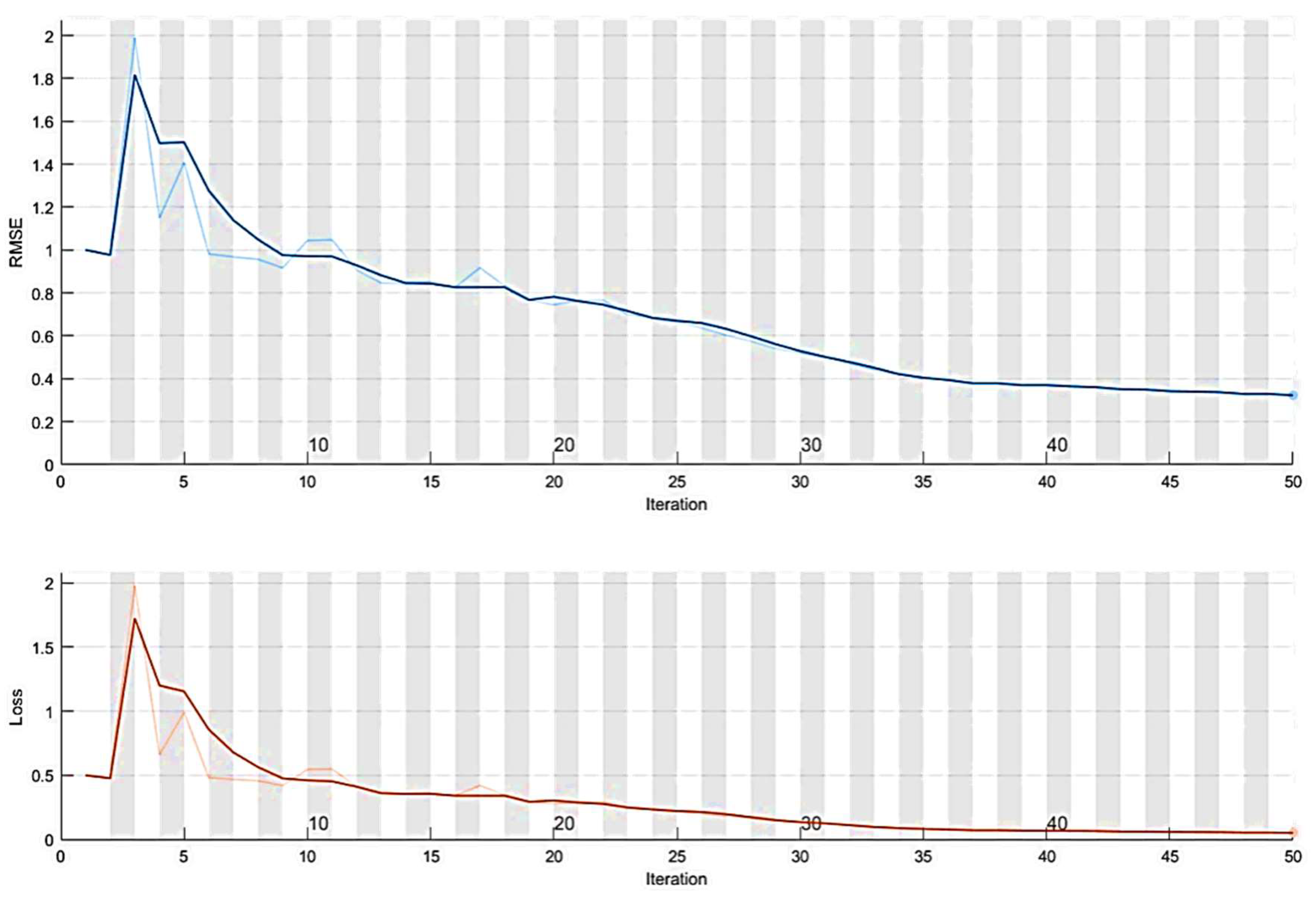
Figure 5 shows the convergence curve of the proposed PHFM model considering the Spanish market summer season week.
From the error outcomes obtained, PHFM generally outperformed, in most of the situations under analysis, the hybrid models under analysis and comparison.
Figure 5 and Table 5 show how the proposed forecasting model is stable and the both the final obtained forecasting error performance measures and training process losses performance gradually converged before the maximum number of iterations considered was reached.
Figure 5 suggests that the RMSE may further trend toward zero if the number of iterations is increased. This means that there might be a margin to improve further the performance of the model by increasing the number of iterations. However, the computational time will also increase with no guarantee that the forecasting error will significantly improve. To tackle this, a broader statistical study with non-parametric analysis may allow the improvement of the results [36].

5. Conclusions

In this work, a PHFM model was proposed for short-term EMP forecasting and was tested considering two real markets’ historical data previously used in other published approaches to validate the PHFM in a fair and valid comparison. Through the analysis of the obtained results, it was possible to verify that the PHFM model demonstrates favorable and above-average results relative to the other models that support the realized comparison.
In this PHFM model, incorporation of the MCS provides a probabilistic perspective of the final forecasting results by analyzing the uncertainty of the results obtained and where they manifest more throughout the historical data. In addition, it was possible to improve and optimize the development of the DEEPSO results before being introduced into the ANFIS chain.
The results obtained from both case studies (Spanish and PJM EMP) revealed the maturity of the PHFM, through assessment by MAPE and weekly error variance criteria. A further analysis considering the introduction of exogenous data, additional error assessment criteria, comparison with other types of probabilistic models, other EMP data, and a broader statistical study with non-parametric analysis is expected to exhibit decreased forecasting errors (associated with the same case studies). This translates to an increase in the reliability for expected applications in real-life scenarios [1].

Author Contributions

Conceptualization, G.J.O. and V.M.A.C.; methodology, V.M.A.C.; validation, M.S.-k., and J.P.S.C.; writing, M.L. and G.J.O.; supervision, J.P.S.C.

Funding

J.P.S. Catalão acknowledges the support by FEDER funds through COMPETE 2020 and by Portuguese funds through FCT, under SAICT-PAC/0004/2015 (POCI-01-0145-FEDER-016434), 02/SAICT/2017 (POCI-01-0145-FEDER-029803) and UID/EEA/50014/2013 (POCI-01-0145-FEDER-006961). M. Lotfi would like to acknowledge the support of the MIT Portugal Program (in Sustainable Energy Systems) by Portuguese funds through FCT, under grant PD/BD/142810/2018.

Conflicts of Interest

The authors declare no conflict of interest.

Nomenclature and Abbreviations

Nomenclature
a ,   b Scaling and translating factors, respectively in wavelet transforms.
A n ,   D n Approximation and details coefficients of order n in wavelet transforms.
C W T x Continuous wavelet transforms.
D W T x Discrete wavelet transforms.
e n s Error variance from probabilistic hybrid forecasting model.
F y ( y ) Cumulative density function from Monte Carlo simulation.
G b e s t , i Best position for differential evolutionary particle swarm optimization.
G b e s t , i * Current best position for differential evolutionary particle swarm optimization.
g Performances function from Monte Carlo simulation.
I Integer variable from Monte Carlo simulation.
i Particle index for differential evolutionary particle swarm optimization.
k Iteration index for differential evolutionary particle swarm optimization
M A P E Mean absolute percentage error.
m ,   n Discrete wavelet transforms counterparts of scaling factors a and b .
N s Dimension of the input data from probabilistic hybrid forecasting model.
n s Time index from probabilistic hybrid forecasting model.
N Size of the swarm for differential evolutionary particle swarm optimization.
p ¯ Electricity market price average results from probabilistic hybrid forecasting model.
p f Probability of failure from Monte Carlo simulation.
p ^ n s Probabilistic hybrid forecasting model output.
p n s Electricity market price data from probabilistic hybrid forecasting model.
Ψ * Complex conjugate continuous domain mother function in wavelet transforms.
Ψ Wavelet transforms mother function
σ γ 2 Variance from Monte Carlo Simulation.
σ e , n s 2 Weekly error variance.
S Set of samples of random variables from Monte Carlo simulation.
T Length of the sampled signal in wavelet transforms.
t Input signal in wavelet transforms.
V i New particle velocity in iteration k for differential evolutionary particle swarm optimization.
w i k * Wight parameters for differential evolutionary particle swarm optimization.
x Time-varying input signal in wavelet transforms (historical data series).
X i New particle position in iteration k for differential evolutionary particle swarm optimization.
X r n i Differential set particle crossover for differential evolutionary particle swarm optimization.
X Historical data set from Monte Carlo simulation.
Y Forecasted results from Monte Carlo simulation.
Abbreviations
ANFISAdaptive neuro-fuzzy inference system.
ARIMAAuto-regressive integrated moving average.
CDFCumulative density function.
DEEPSOHybrid particle swarm optimization.
EMPElectricity market prices.
EPAEvolutionary particle swarm optimization algorithm.
FISFuzzy inference system.
GAGenetic algorithm.
HEHybrid evolutionary algorithm.
HISHybrid intelligent system.
HPFMHybrid probabilistic forecasting model.
HPMHybrid particle swarm optimization model.
MAPEMean absolute percentage error.
MCSMonte Carlo Simulation.
MICNNMutual information cascaded artificial neural networks.
NNArtificial neural network.
PDFProbability density function.
PJMPennsylvania-New Jersey-Maryland electricity market.
PSOParticle swarm optimization.
WTWavelet transforms.

References

  1. Nowotarski, J.; Weron, R. Recent Advances in Electricity Price Forecasting: A Review of Probabilistic Forecasting. HSC Res. Rep. 2016, 81, 1548–1568. [Google Scholar] [CrossRef]
  2. Khooban, M.-H. Secondary Load Frequency Control of Time-Delay Stand-Alone Microgrids With Electric Vehicles. IEEE Trans. Ind. Electron. 2018, 65, 7416–7422. [Google Scholar] [CrossRef]
  3. Li, X.R.; Yu, C.W.; Ren, S.Y.; Chiu, C.H.; Meng, K. Day-Ahead Electricity Price Forecasting Based on Panel Cointegration and Particle Filter. Electr. Power Syst. Res. 2013, 95, 66–76. [Google Scholar] [CrossRef]
  4. Dufo-López, R.; Bernal-Agustín, J.L.; Monteiro, C. New Methodology for the Optimization of the Management of Wind Farms, Including Energy Storage. Appl. Mech. Mater. 2013, 330, 183–187. [Google Scholar] [CrossRef]
  5. Ren, Y.; Suganthan, P.N.; Srikanth, N. Ensemble Methods for Wind and Solar Power forecasting—A State-of-the-Art Review. Renew. Sustain. Energy Rev. 2015, 50, 82–91. [Google Scholar] [CrossRef]
  6. Okumus, I.; Dinler, A. Current Status of Wind Energy Forecasting and a Hybrid Method for Hourly Predictions. Energy Convers. Manag. 2016, 123, 362–371. [Google Scholar] [CrossRef]
  7. Yadav, A.; Peesapati, R.; Kumar, N. Electricity Price Forecasting and Classification Through Wavelet–Dynamic Weighted PSO–FFNN Approach. IEEE Syst. J. 2017, 29, 1–10. [Google Scholar]
  8. Jafari, M.; Malekjamshidi, Z.; Zhu, J.; Khooban, M.-H. Novel Predictive Fuzzy Logic-Based Energy Management System for Grid-Connected and Off-Grid Operation of Residential Smart Micro-Grids. IEEE J. Emerg. Sel. Top. Power Electron. 2018. [Google Scholar] [CrossRef]
  9. Osório, G.; Gonçalves, J.; Lujano-Rojas, J.; Catalão, J.; Osório, G.J.; Gonçalves, J.N.D.L.; Lujano-Rojas, J.M.; Catalão, J.P.S. Enhanced Forecasting Approach for Electricity Market Prices and Wind Power Data Series in the Short-Term. Energies 2016, 9, 693. [Google Scholar] [CrossRef]
  10. Catalão, J.P.S.; Pousinho, H.M.I.; Mendes, V.M.F. Short-Term Electricity Prices Forecasting in a Competitive Market by a Hybrid Intelligent Approach. Energy Convers. Manag. 2011, 52, 1061–1065. [Google Scholar] [CrossRef]
  11. Weron, R. Electricity Price Forecasting: A Review of the State-of-the-Art with a Look into the Future. Int. J. Forecast. 2014, 30, 1030–1081. [Google Scholar] [CrossRef]
  12. Contreras, J.; Espínola, R.; Nogales, F.J.; Conejo, A.J. ARIMA Models to Predict Next-Day Electricity Prices. IEEE Trans. Power Syst. 2003, 18, 1014–1020. [Google Scholar] [CrossRef]
  13. Catalão, J.P.S.; Mariano, S.J.P.S.; Mendes, V.M.F.; Ferreira, L.A.F.M. Short-Term Electricity Prices Forecasting in a Competitive Market: A Neural Network Approach. Electr. Power Syst. Res. 2007, 77, 1297–1304. [Google Scholar] [CrossRef]
  14. Kim, M.K. Short-Term Price Forecasting of Nordic Power Market by Combination Levenberg–Marquardt and Cuckoo Search Algorithms. IET Gener. Transm. Distrib. 2015, 9, 1553–1563. [Google Scholar] [CrossRef]
  15. Amjady, N.; Hemmati, M. Day-Ahead Price Forecasting of Electricity Markets by a Hybrid Intelligent System. Eur. Trans. Electr. Power 2009, 19, 89–102. [Google Scholar] [CrossRef]
  16. Miranian, A.; Abdollahzade, M.; Hassani, H. Day-Ahead Electricity Price Analysis and Forecasting by Singular Spectrum Analysis. IET Gener. Transm. Distrib. 2013, 7, 337–346. [Google Scholar] [CrossRef]
  17. Alamaniotis, M.; Bargiotas, D.; Bourbakis, N.G.; Tsoukalas, L.H. Genetic Optimal Regression of Relevance Vector Machines for Electricity Pricing Signal Forecasting in Smart Grids. IEEE Trans. Smart Grid 2015, 6, 2997–3005. [Google Scholar] [CrossRef]
  18. Osório, G.J.; Matias, J.C.O.; Catalão, J.P.S. Electricity Prices Forecasting by a Hybrid Evolutionary-Adaptive Methodology. Energy Convers. Manag. 2014, 80, 363–373. [Google Scholar] [CrossRef]
  19. Tahmasebifar, R.; Sheikh-El-Eslami, M.K.; Kheirollahi, R. Point and Interval Forecasting of Real-Time and Day-Ahead Electricity Prices by a Novel Hybrid Approach. IET Gener. Transm. Distrib. 2017, 11, 2173–2183. [Google Scholar] [CrossRef]
  20. Lee, D.; Shin, H.; Baldick, R. Bivariate Probabilistic Wind Power and Real-Time Price Forecasting and Their Applications to Wind Power Bidding Strategy Development. IEEE Trans. Power Syst. 2018, 33, 6087–6097. [Google Scholar] [CrossRef]
  21. Moreira, R.; Bessa, R.; Gama, J. Probabilistic Forecasting of Day-Ahead Electricity Prices for the Iberian Electricity Market. In Proceedings of the 2016 13th International Conference on the European Energy Market (EEM), Porto, Portugal, 6–9 June 2016; pp. 1–5. [Google Scholar]
  22. Rafiei, M.; Niknam, T.; Khooban, M.-H. Probabilistic Forecasting of Hourly Electricity Price by Generalization of ELM for Usage in Improved Wavelet Neural Network. IEEE Trans. Ind. Inform. 2017, 13, 71–79. [Google Scholar] [CrossRef]
  23. Miranda, V.; Alves, R. Differential Evolutionary Particle Swarm Optimization (DEEPSO): A Successful Hybrid. In Proceedings of the 2013 BRICS Congress on Computational Intelligence and 11th Brazilian Congress on Computational Intelligence, Ipojuca, Brazil, 8–11 September 2013; pp. 368–374. [Google Scholar]
  24. Rafiei, M.; Niknam, T.; Khooban, M.H. A Novel Intelligent Strategy for Probabilistic Electricity Price Forecasting: Wavelet Neural Network Based Modified Dolphin Optimization Algorithm. J. Intell. Fuzzy Syst. 2016, 31, 301–312. [Google Scholar] [CrossRef]
  25. Rafiei, M.; Niknam, T.; Khooban, M.H. Probabilistic Electricity Price Forecasting by Improved Clonal Selection Algorithm and Wavelet Preprocessing. Neural Comput. Appl. 2017, 28, 3889–3901. [Google Scholar] [CrossRef]
  26. Haque, A.U.; Mandal, P.; Meng, J.; Srivastava, A.K.; Tseng, T.-L.; Senjyu, T. A Novel Hybrid Approach Based on Wavelet Transform and Fuzzy ARTMAP Networks for Predicting Wind Farm Power Production. IEEE Trans. Ind. Appl. 2013, 49, 2253–2261. [Google Scholar] [CrossRef]
  27. Catalao, J.P.S.; Pousinho, H.M.I.; Mendes, V.M.F. Hybrid Wavelet-PSO-ANFIS Approach for Short-Term Electricity Prices Forecasting. IEEE Trans. Power Syst. 2011, 26, 137–144. [Google Scholar] [CrossRef] [Green Version]
  28. Kennedy, J.; Eberhart, R. Particle Swarm Optimization. In Proceedings of the ICNN’95—International Conference on Neural Networks, Perth, Australia, 27 November–1 December 1995; Volume 4, pp. 1942–1948. [Google Scholar]
  29. Castillo, O.; Martínez-Marroquín, R.; Melin, P.; Valdez, F.; Soria, J. Comparative Study of Bio-Inspired Algorithms Applied to the Optimization of Type-1 and Type-2 Fuzzy Controllers for an Autonomous Mobile Robot. Inf. Sci. 2012, 192, 19–38. [Google Scholar] [CrossRef]
  30. Soliman, O.S.; Mohamed, S.M.; Ramadan, E.A. A Bio-Inspired Memetic Particle Swarm Optimization Algorithm for Multi-Objective Optimization Problems. In Proceedings of the 2012 Third International Conference on Innovations in Bio-Inspired Computing and Applications, Kaohsiung, Taiwan, 26–28 September 2012; pp. 127–132. [Google Scholar]
  31. Hassan, R.; Cohanim, B.; de Weck, O.; Venter, G. A Comparison of Particle Swarm Optimization and the Genetic Algorithm. In Proceedings of the 46th AIAA/ASME/ASCE/AHS/ASC Structures, Structural Dynamics and Materials Conference, Austin, TX, USA, 18–21 April 2005; p. 1897. [Google Scholar]
  32. Miranda, V.; Cerqueira, C.; Monteiro, C. Training a FIS with EPSO under an Entropy Criterion for Wind Power Prediction. In Proceedings of the 2006 International Conference on Probabilistic Methods Applied to Power Systems, Stockholm, Sweden, 11–15 June 2006; pp. 1–8. [Google Scholar]
  33. Taieb, S.B.; Atiya, A.F. A Bias and Variance Analysis for Multistep-Ahead Time Series Forecasting. IEEE Trans. Neural Netw. Learn. Syst. 2016, 27, 62–76. [Google Scholar] [CrossRef]
  34. Banerjee, B.; Jayaweera, D.; Islam, S. Modelling and Simulation of Power Systems. In Studies in Systems, Decision and Control; Springer: Berlin/Heidelberg, Germany, 2016; Volume 57, pp. 15–28. [Google Scholar]
  35. Lidebrandt, T. Variance Reduction Three Approaches to Control Variates; Mathematical Statistics; Stockholm University: Stockholm, Sweden, 2007. [Google Scholar]
  36. Demšar, J. Statistical Comparisons of Classifiers over Multiple Data Sets. J. Mach. Learn. Res. 2006, 7, 1–30. [Google Scholar]
Figure 1. Basic flowchart structure of the Monte Carlo simulation used.
Sustainability 11 00057 g001
Figure 2. Flowchart structure of the probabilistic hybrid forecasting model.
Sustainability 11 00057 g002
Figure 3. Spring (a), Summer (b), Fall (c), and Winter (d) weeks from the Spanish market in 2002. Forecasted EMP in solid black line; real EMP in blue dashed line; fading grey areas reflect uncertainty levels obtained by MCS from high uncertainty (lighter) to low uncertainty (darker).
Sustainability 11 00057 g003aSustainability 11 00057 g003b
Figure 4. Week of 22–28 February from the PJM market. Forecasted EMP in solid black line; real EMP in blue dashed line; fading grey areas reflect uncertainty levels obtained by MCS from high uncertainty (lighter) to low uncertainty (darker).
Sustainability 11 00057 g004
Figure 5. Convergence plot of the root mean square error (upper/blue) and the losses (lower/orange), for the Spanish market winter case. Smoothing training results are in solid bold lines and the real training results are in light faded lines.
Sustainability 11 00057 g005
Table 1. Main parameters’ description that compose the probabilistic hybrid forecasting model.
ComponentParameterValue
WTWT directionrow
(Re) Decomposition level3
WT mother functionDb3”, “Db4
Analysis noise toolsqtwolog”, ”minimaxi
Rescaling thresholdsone”, “sln”, “mln
DEEPSOSharing information probability0.1
Early inertia weight0.01–0.9
Ending inertia weight0.01–0.1
Starting swarm cognitive weights1–4
Starting swarm spreading process1–4
Starting spreading acceleration1–4
Population size168
Minimum point of new locationSet of Min. inputs
Maximum point of new locationSet of Max. inputs
Cognitive parameter0.1
Iterations per simulation50–1000
ANFISMembership rules2–15
Number of iterations per simulation2–50
Membership function bell“pimf”, “trimf
Table 2. Mean absolute percentage error comparison for the Spanish electricity market prices in (%).
[9,13,18]SpringSummerFallWinterAverage
NN (2007)5.3611.4013.655.238.91
HIS (2009)6.067.077.477.306.97
MICNN (2012)4.286.475.274.515.13
EPA (2011)4.106.396.403.595.12
HPM (2016)3.706.166.283.554.92
HEA (2014)3.335.384.974.294.18
PHFM (2018)4.135.214.774.484.65
Table 3. Weekly error variance comparison for the Spanish electricity market prices in (%).
[9,13,18]SpringSummerFallWinterAverage
NN (2007)0.00180.01090.01360.00170.0070
HIS (2009)0.00490.00290.00310.00340.0036
MICNN (2012)0.00140.00330.00220.00140.0021
EPA (2011)0.00160.00480.00320.00120.0027
HPM (2016)0.00160.00370.00320.00080.0019
HEA (2014)0.00110.00260.00140.00080.0015
PHFM (2018)0.00160.00210.00100.00110.0014
Table 4. Mean absolute percentage error and weekly error variance comparison for the Pennsylvania-New Jersey-Maryland electricity market prices in (%).
[9,13,18]MAPE (%)Variance
HIS (2009)7.300.0031
EPA (2011)6.400.0032
HEA (2014)3.080.0017
PHFM (2018)5.880.0026
Table 5. Performance of proposed forecasting model for all test cases: Mean, standard variance, and maximum and minimum errors.
Test CaseMeanStandard VarianceMaximum ErrorMinimum Error
Winter (Spanish EMP)42.588.1013.64−3.97
Spring (Spanish EMP)43.968.2710.59−4.88
Summer (Spanish EMP)40.3410.5712.89−5.07
Fall (Spanish EMP)32.9310.615.75−3.68
Winter (PJM EMP)53.2811.8110.27−9.10

