Article

Evaluating Hydrological Models for Deriving Water Resources in Peninsular Spain

by
Julio Pérez-Sánchez
1,*,
Javier Senent-Aparicio
1,
Francisco Segura-Méndez
1,
David Pulido-Velazquez
1 and
Raghavan Srinivasan
2
1
Department of Civil Engineering, Catholic University of San Antonio, Campus de los Jerónimos, s/n, Guadalupe, 30107 Murcia, Spain
2
Spatial Science Laboratory, Ecosystem Science and Management Department, Texas A & M University, College Station, TX 77843, USA
*
Author to whom correspondence should be addressed.
Sustainability 2019, 11(10), 2872; https://0-doi-org.brum.beds.ac.uk/10.3390/su11102872
Submission received: 24 April 2019 / Revised: 13 May 2019 / Accepted: 15 May 2019 / Published: 20 May 2019
(This article belongs to the Special Issue Watershed Processes under Changing Climate)

Abstract

:
Water availability is essential for the appropriate analysis of its sustainable management. We performed a comparative study of six hydrological balance models (Témez, ABCD, GR2M, AWBM, GUO-5p, and Thornthwaite-Mather) in several basins with different climatic conditions within Spain in the 1977–2010 period. We applied six statistical indices to compare the results of the models: the Akaike information criterion (AIC), the Bayesian information criterion (BIC), Nash–Sutcliffe model efficiency coefficient (NSE), coefficient of determination (R2), percent bias (PBIAS), and the relative error between observed and simulated run-off volumes (REV). Furthermore, we applied the FITEVAL software to determine the uncertainty of the model. The results show that when the catchments are more humid the obtained results are better. The GR2M model gave the best fit in peninsular Spain in a UNEP aridity index framework above 1, and NSE values above 0.75 in a 95% confidence interval classify GR2M as very good for humid watersheds. The use of REV is also a key index in the assessment of the margin of error. Flow duration curves show good performance in the probabilities of exceedance lower than 80% in wet watersheds and deviations in low streamflows account for less than 5% of the total streamflow.

Graphical Abstract

1. Introduction

Water resources assessment is key to the analysis of catchment management [1]. The cost and irregular distribution of worldwide water resources are evident. Even in parts of the planet where water resources are abundant, the problems of availability or scarcity are common due to, largely, weak water management practices and anthropic activities [2]. The development of models to study water availability is a complex task that presents a fundamental scientific challenge. Complex cases, in particular, occur in arid and semi-arid regions, where precipitation is limited or irregular and evapotranspiration (ET) rates are high. Hydrological balance models are used to reconstruct historical series and predict future ones [3]. They are based on the principle of mass conservation or the continuity equation [4], which considers that the difference of inputs and outputs will be reflected in water storage in the catchment [5,6].
The concept of hydrological balance models was first introduced by Thornthwaite [7] and Thornthwaite and Mather [8]. They proposed two different conceptual models based on two parameters: soil moisture capacity and water excess above the maximum soil moisture storage capacity. These models demonstrated a good fit to estimate monthly run-off [9] and have formed the basis of many other two-parameter hydrological models [9,10,11,12,13,14]. There are also water balance models that comprise more than two parameters [15,16,17]. However, Xiong and Guo [10] showed that their proposed two-parameter model in China performed as well as a five-parameter model. To date, several studies have shown that many models produce similar results to previous ones [18,19,20,21]. In a lumped water balance model, catchment parameters and variables are averaged in space, so hydrological processes are approached by conceptual solutions formulated using semi-empirical equations. The system is described using different reservoirs, the moisture content of which depends on the relationships (physical and empirical) between them [22]. A lumped hydrological balance model may have only three or four parameters [9,22,23] and can be implemented with several lines of computer code, whereas a complex model may have more than 20 parameters [24]. Some examples of lumped models are the ABCD model [14,25,26,27], GR2M [28,29], Sacramento [30], Guo-5p [10,31], Témez [32,33,34,35,36], Thornwaite-Mather [37,38,39], IHACRES [40], SIMHYD [41], GR4J [42], AWBM [43,44,45,46,47], and SMAR [48]. More examples of rainfall run-off models can be found in Singh [49] and Singh and Frevert [50].
With the development of computer aided tools and more detailed information, there is an increasing trend toward using distributed or semi-distributed models [51,52]. They provide more detailed distributed results on a catchment scale approximating heterogeneities of the system. Following these assumptions, many complex models have been developed that are assumed to be capable of simulating environmental change. These spatially explicit and physically-based model approaches are often criticized because the necessary a priori estimation of model parameters is difficult [53,54], and uncertainty at high resolution may diminish potential gains in prediction accuracy [55]. Thus, efficient calibration of the models is difficult due to the spatially distributed nature of those models, showing, sometimes, a decrease in efficiency [56], and lumped models can provide a more appropriate alternative [57]. Moreover, lumped models do not need as much data as distributed models, and the complexity and requirements to process them are lower. The calibration of the lumped parameter models is much less time consuming and produces higher overall model performance in comparison to the more complex distributed models [58]. Notwithstanding, recent studies in distributed hydrologic models have developed methodology approaches that improve the limitations mentioned above. Samaniego et al. [59] used a multiscale parameter regionalization (MPR) technique in a fully spatially distributed conceptual hydrologic model, resulting in the limitation of a number of model parameters and the transferability of the global parameters at a coarser scale to a finer scale, meaning that there is a substantial shortcoming in the calibration procedure. Beck et al. [60] developed a scheme for the regionalization of model parameters at the global scale, resulting in HBV parameter maps, such as ancillary data that are available via www.gloh2o.org.
Notwithstanding, despite the simplicity of lumped models, they performed well in many studies [61,62,63,64]. Other studies that have compared lumped and distributed models confirmed that both of them lead to similar accuracy [65,66,67,68,69,70,71,72,73,74,75] and that lumped models can be calibrated more efficiently [76]. Vansteenkiste et al. [77] learned that in a Belgian catchment, the lumped models perform better than the distributed ones in seasonal events and in terms of overall water balance, with very low discrepancies in the subflow volumes in comparison to the distributed models. Furthermore, lumped models provide a valuable integrated view of the basin outlet response, as concluded by the Distributed Model Intercomparison Project for the Oklahoma region by Reed et al. [72] and Smith et al. [66]. Martínez-Santos and Andreu [78] used lumped and distributed approaches to model natural recharge in semi-arid aquifers in Spain, and even though both approaches performed similarly, the lumped models exhibited a better agreement with field records.
Therefore, spatial discretization is not the only determinant of the simulation’s quality. The choice of model is dictated by the modelling purpose. When flow at the catchment outlet is the main required goal in water resources management, lumped models may be the best choice, but when spatially explicit predictions or land use change predictions are required, a (semi-)distributed model would be more appropriate, although land use changes can also be carried out in a lumped model by means of transfer functions [68]. Recently, lumped models have been used, among other purposes, to obtain detailed assessments of surface flow, water balance components, and the impact of climate change [79,80] to estimate catchment discharge [81,82,83], and to explore transferability under contrasting climate conditions [84,85].
In this study, choosing the models is mainly based on known performance in different climatic regions, both in Spain and Europe, and structural diversity (i.e., 3–6 free parameters and 2–4 storage units). However, an inadequate complexity often results in over-parameterization [19,86,87], so the models with too many parameters (more than 6) are excluded from this study. Thus, the Témez model has been widely used in Spanish catchments [88,89,90,91] and by the Spanish government in water management [92]. The widely used ABCD model has proven to have reasonable predictability and has been compared with numerous monthly water balance models, thus leading to its recommendation [27,93,94,95,96]. Vandewiele and Xu [17] also found that the ABCD model compares favorably with other more recent monthly water balance models in Belgium. Currently, the ABCD model has been found to have the best performance in the Segura River basin in southern Spain [97]. The GR2M model is widely used in France in all of its different versions [98]. Wriedtand and Bouraoiu [99] used this model in 492 catchments in Germany, France, Spain, and Portugal and obtained high NSE in the center and north of Spain and in Central European basins. The AWBM is one of the most widely used rainfall run-off models in Australia [46], but it has been used in different global catchments [25,100,101], both humid and dry basins, and it has proven to have performance similar to the distributed models [102]. The Thornthwaite and Mather water balance model is valid as a water accounting procedure when only reduced information about hydrologic inputs and aquifer characteristics is available, as applied by Peranginangin et al. [103]. It has been successfully used in different water balance research studies in Spain [104,105,106,107]. Finally, Guo-5p is an adaptation of Thornthwaite and Mather’s model with five parameters, so it was chosen to compare with the latter. Its use is particularly recommended in humid and semi-humid regions [10,31].
Our primary objective in this study is to use model predictions for the assessment of water resources, as the first step in predicting future resources under climate change. This should predict and solve problems related to the quantity and quality of water, as well as ensure its sustainable use. Furthermore, the following must also be considered: the population growth rate, increasing demand, depleted fluvial networks, the requirements concerning ecological flow, and the reduction in the amount of groundwater. Thus, efficient water management becomes an essential issue due to global scarcity. Our work is mainly focused on the comparative analysis of hydrological models and their ability to predict and quantify outflows on the basis of different watersheds in Spain, where the wide range of climates is optimal for such hydrological research.
The first step, which is developed in this research, addresses the issue of comparing and selecting, using different metrics and graphics, the water balance model that has the best fit according to our goal: water resources assessment. Although, as previously stated, there are many studies that compare different hydrological models, we have used a full set of statistical methods in order, not only to verify the feasibility and the performance of these models in different climatic areas, but also to assess the usefulness of the combination of different goodness-of-fit tools depending on the purpose of the study. Therefore, six lumped water balance models were evaluated in 16 basins located in different climatic regions of Spain, where a long-time series of climatic and natural streamflow data are available (more than 30 years). We intended to calibrate parsimonious approaches to estimate natural streamflow series, and we intended to generate a series that represents the stochastic variability of the rainfall process. These series can be used as inputs of management models to assess the operation of water resource systems. In these cases, we need long time series of inflows (natural streamflows) to account for the influence of the hydrology’s stochastic behaviors in the reliabilities of the demand supply [108,109]. Our aim is to select the models with the best fit and to assess the comparison methods used according to the region’s characteristics. We structured the paper’s contents as follows. Section 2 introduces the data and methodology; Section 3 presents the results and the discussion; and Section 4 highlights the main conclusions.

2. Materials and Methods

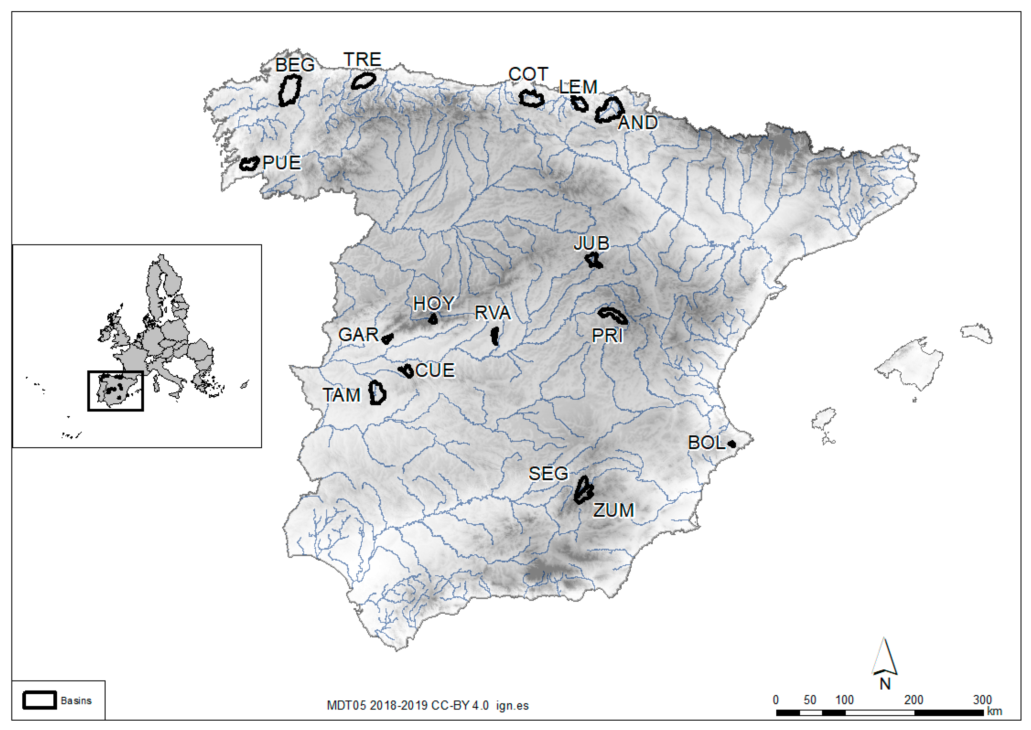
2.1. Study Area and Data

Spain is the second largest country in Western Europe, with a territory covering 505,990 km2, a dense network of rivers with many branches and a large number of aquifers. This disparity within the Iberian Peninsula is optimal for hydrological research. Spain features a wide range of climates due to its position between the European temperate zone and the subtropical zone. It also includes some of the rainiest areas in Europe in the northeast and the driest areas in the southeast, with a marked summer drought. To ensure the validity of the results, the 16 selected catchments are in the natural regime. They are located all over the country, as shown in Figure 1. Thus, the geographic and climatic variety in Spain are reflected wherever data were available.
Their altitudes vary from 1632 to 342 m above sea level (MASL), and catchment areas range from 29–837 km2 with an average of 300 km2 (Table 1). There is no southwestern catchment in this study due to the lack of data in this area, where most gauging stations have data for a period of less than 10 years. As shown in Table 1, the average temperatures range from 8–16 °C, depending on the latitude and average altitude of the catchment, with a positive gradient to the south. With regards to the rainfall regime, the highest yearly precipitation occurs in the north of Spain, where average temperatures are lower, and consequently, ET is less. However, in the southern half of the Iberian Peninsula, ET is generally higher than precipitation, especially in the lowlands, which have an average altitude of less than 600 m.
The study area comprises the most common climate groups in the Iberian Peninsula, according to Köppen’s [110,111,112] classification: Bsk. (Cold semi-arid), Csb. (Warm-summer Mediterranean), Csa. (Hot-summer Mediterranean climate), Cfb. (Temperate oceanic), and UNEP aridity index [113]. This index (AIU) is defined by Equation (1).
AI U = P PET
where P is the average annual precipitation and PET is the potential evapotranspiration. The thresholds that define the various degrees of aridity depend on the value of AIU: hyper-arid (AIU < 0.05), arid (0.05 < AIU < 0.20), semi-arid (0.20 < AIU < 0.50), dry sub-humid (0.50 < AIU < 0.65), humid sub-humid (1.00 < AIU < 0.65), and humid (AIU > 1.00). Among the 16 catchments studied, nine are considered humid; thus, their AIU exceeds one, and five of them even have an aridity index near to or above 2. All are located in northern Spain. Despite the rainfall gradient from the northwest to the southeast, the SEG and ZUM catchments are classified as humid sub-humid due to their altitude above 1000 MASL. The BOL catchment, which is close to the Mediterranean Sea, is the only eastern dry sub-humid region of the regions studied; thus, the other dry sub-humid catchments (TAM and CUE) are located in the center of the Iberian Peninsula. The only semi-arid region in the studied catchments is RVA, the average altitude of which is approximately 600 MASL.
We carried out an analysis of land cover variations in the period 1990–2012 in the watersheds (Table 1) in order to consider their influence in models both in the calibration and the validation. Notwithstanding, nearly all watersheds show a variation below 5%, which will not affect the main conclusions. However, RVA and LEM land cover have changed 9.18% and 19.12%, respectively, in the available data period, and will be further discussed.
Precipitation and PET data series in each basin are from a 33-year period (1977–2010). We obtained the data from the official monthly series provided by the CEDEX (Centre of Studies and Experimentation of Civil Works) for the Spanish government [114] at a spatial resolution of 500 × 500 m2 [115]. The model has been validated at more than 100 control points [91] and used in Spain for water resources assessment, in the White Paper Book of Waters [89], and in several studies [116,117,118]. Natural streamflow data in each catchment are available for the same period. They come from measurements at gauging stations in the official Spanish network. Missing streamflow values range from 2–8% in the stations considered. We obtained digital elevation models and land cover variations [119] from the National Geographical Institute of Spain [120]. Furthermore, in order to assess hierarchical order of the main river courses of the basins, the Pfastetter code is considered. As shown in Table 2, the range of the code of the basins studied varies between 913685 and 104080, indicating a wide variety of topological location within the watershed.

2.2. Methodology

The methods we used in this investigation are based on the identification of the hydrological models that best fit each catchment considered. Six monthly water balance models were used: Témez, ABCD, GR2M-1994, Australian Water Balance Model (AVBM), Guo-5p, and Thornwaite-Mather. All these models use precipitation and PET as input data. We assessed the goodness of fit for the six models using various model selection criteria for the purpose of establishing a robust methodology that can validate the conclusions obtained and its application in other different regions. Accepting the fact that models only approximate reality, our objective was to determine which of the candidate models best approximates the data. Because the field of information theory is used to quantify or measure the expected value of the information, we used the information theoretic approach to derive the two most-commonly-used criteria in model selection: the Akaike information criterion (AIC) [121,122] and the Bayesian information criterion (BIC) [123]. The difference between the BIC and the AIC is the greater penalty imposed for the number of parameters by the former than the latter. Alternatively, and based on Moriasi et al. [124] and Bressiani et al. [125], we established a grading method to evaluate the good performance of the model based on the NSE, R2, and PBIAS values. We also analyzed the relative error between observed and simulated run-off volumes and the flow duration curves (FDCs) in the studied period to assess both low-flows and high-flows. Finally, we carried out the uncertainty of the model selected in each watershed with the FITEVAL software [126]. All of these hydrological models are defined with four parameters, except Thornwaite-Mather (three parameters) and Guo-5p (five parameters). Through all phases of the hydrological cycle, the models conduct different moisture balances according to the different processes in a hydrological system. The processes are governed by the continuity principle and mass balance and remain regulated by the specific laws of division and the transfer between the reservoirs of each model [90].

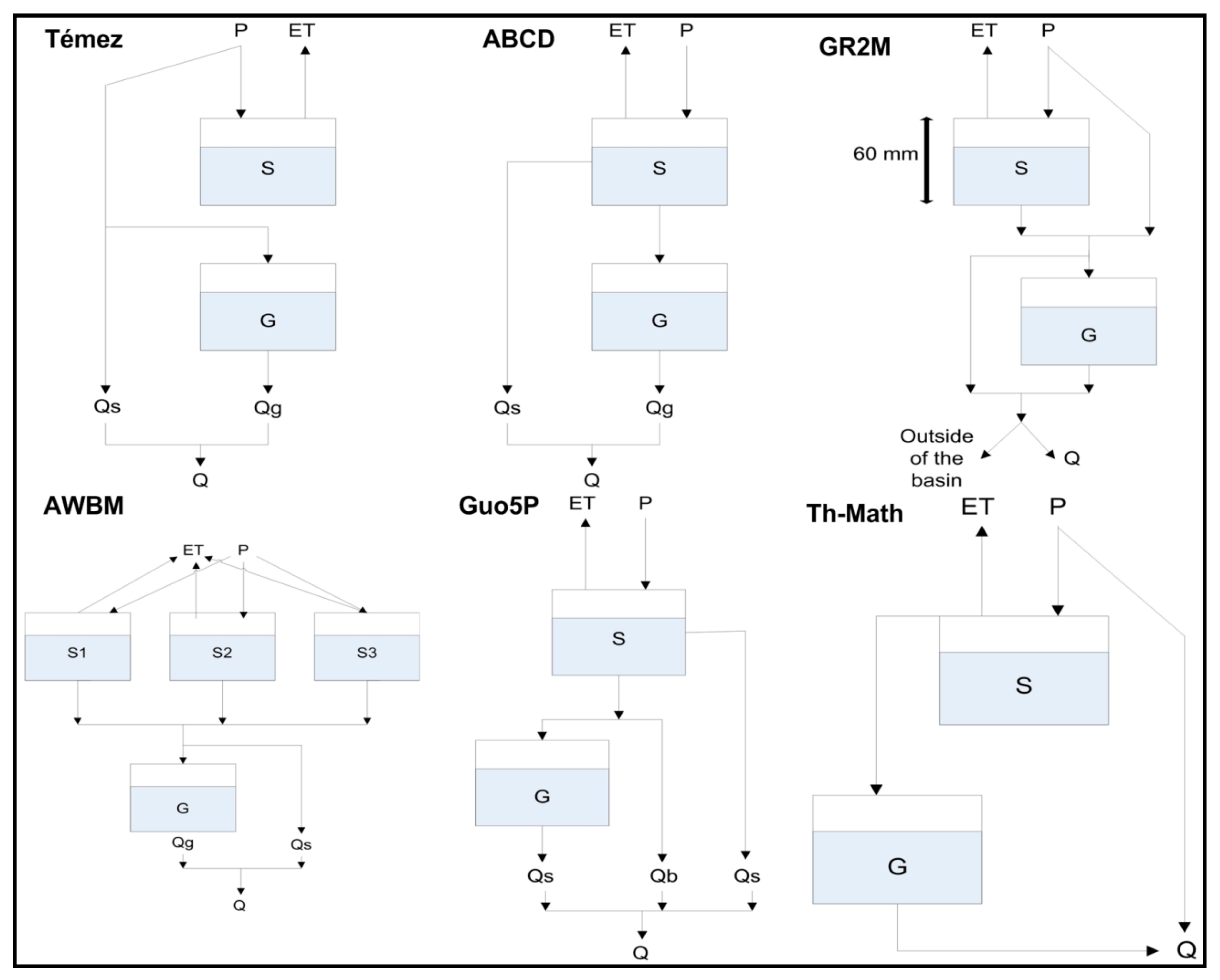
2.2.1. Water Balance Models

Témez Model

Témez [127] developed the Témez model, which has been widely used in Spanish catchments [88,89,90,91] and by the Spanish government in water management [92]. This model considers the system to be divided into two zones (Figure 2): the upper or non-saturated zone (S) and the lower or saturated zone (G). Some of the precipitation (P) drains directly into the river or through the aquifer, while the remainder is converted into ET. Excess is divided into run-off (Qs) through river networks at the present time, and infiltration to aquifers, draining one part (Qg) at the present time, with the rest remaining in the groundwater storage tank (G) for drainage at a later date (Figure 2).

ABCD Model

The ABCD 4-parameter model [9] introduces a different formulation in the ET process and allows for a water surplus even though the soil moisture tank (S) is not full yet. As shown in Figure 2, this model also considers two storage tanks: upper storage (S), or soil, and groundwater storage (G). The upper storage tank (S) has two outputs: run-off (Qs) and infiltration. Thus, the model has two inputs, precipitation (P) and PET, and their outputs are soil moisture content at the end of the month (S), monthly available water, ET, run-off (Qs), infiltration, groundwater run-off (Qb), monthly groundwater storage (G), and total run-off (Q) (Figure 2).

GR2M-1994 Model (GR4-1994)

This model [11] was developed in the 1990s by the CEMAGREF (Centre of Agricultural and Environmental Research of France). It is also based on monthly precipitation and ET [128]. Afterwards, the model evolved into different versions, such as GR1A, GR2M, GR3J, and GR4J, denominated by the number of required parameters and with the last letter denominating the period considered: J (daily), M (monthly), or A (yearly). GR2M transforms precipitation into run-off through the implementation of two equations: production and transfer functions [128,129]. Initially, P and ET are balanced and precipitation is distributed between the upper storage tank (S) with a limited capacity and groundwater storage tank (G) [130]. Nief et al. [131] showed that model parameters are robust to non-stationary rainfall series, and calibrated parameter values are highly correlated with land use. Like previous models, monthly P and ET are the inputs, and the operating diagram is shown in Figure 2.

AWBM Model

The AWBM was also developed in the 1990s and is the most commonly used water balance method in Australia [46]. This model has three surface water-storage tanks (S1, S2, and S3). The water balance of each is estimated independently, resulting in three surpluses. One part of these surpluses is transformed into run-off (Qs), and the other part percolates to a groundwater storage tank or aquifer (G), which in turn goes to groundwater run-off (Qg). Total flow (Q) is obtained by adding both run-offs (Figure 2).

Guo Model (Five Parameters)

This model was developed to estimate the run-off in 70 catchments in southern China. It has a similar performance to the two-parameter Guo model, and its use is particularly recommended in humid and semi-humid regions [10,31]. Precipitation and evapotranspiration (P and ET) are the input data, on the basis of which the remaining parameters are estimated: ET, soil water storage (S), water surpluses, surface run-off (Qs), subsurface run-off (Qb), aquifer recharge, groundwater storage (G), groundwater run-off (Qg), and total flow (Q).

Thornthwaite-Mather Model

This model was developed by Thornwaite and Mather [8,132] in the early 1940s for the Delaware River, and many water balance models are based on it. The model distinguishes two water storage tanks: surface (S) and groundwater (G), which lead to the output flow (Q) through different calculations.
More detailed information about model performance and governing model equations is provided in Appendix A.

2.2.2. Goodness-of-Fit Tests

The study period is 34 years (1977–2010). We employed three years for warming up, and the other 30 years, starting October 1980, for calibration and validation, applying the split sample test proposed by KlemeŠ [133]. Therefore, the data series from 1980–2010 (30 years) was divided into two sets. We used the first 15 years (1980–1995) for calibration, and the remaining 15 years (1995–2010) for model validation, namely as a security measure of calibration. As suggested by Kirchner [87], both series (calibration and validation) should exhibit different revealing behaviors with regards to the representativeness and reliability of modelling results and their deployment. Thus, we provided a comparison of precipitation values in both calibration and validation periods. We conducted calibration of all models’ parameters by comparing the predicted data with the observed data. The optimal value for each parameter is the value that minimizes the differences between both flow series and the objective function that minimizes the sum of the square of deviations. We used the generalized reduced gradient as the optimization algorithm [134], which searches for the extreme values of the functions by the generalized reduced gradient algorithm method (GRG2) [135,136,137,138]. We used the multi-start method to find a globally optimal solution [139,140]. The multi-start method operates by generating candidate starting point values randomly selected between the bounds specified for the variables. These points are then grouped into clusters that are run repeatedly to capture the locally optimal solution. We used a Bayesian test to determine whether the process should continue or stop. As the number of runs of the non-linear iterations increases, the probability that the globally optimal solution has been found also increases 100%. For most non-linear problems, this method will at least yield very good solutions [140]. In this study, 1000 starting points have been used for each model and watershed. Once the model was calibrated and the parameters validated, we executed the predictive stage.
To evaluate model accuracy, six statistic indices were obtained: AIC [121,122], BIC [123], NSE [141], R2 [142], PBIAS [143], and REV [144]. The formulas used are presented in Equations (2)–(11).
AIC = 2 log   L ( Ŏ ) + 2 k
BIC = 2 log   L ( Ŏ ) + klog   n
where Ŏ is the set (vector) of model parameters
L( Ŏ ) is the likelihood of the candidate model given the data when evaluated at the maximum likelihood estimate of θ. Root mean squared error of the model output (RMSE) was used in this study; k is the number of estimated parameters in the candidate model, and n is the sample size
NSE = 1 i = 1 n ( Q obs , i Q sim , i ) 2 i = 1 n ( Q obs , i Q obs ¯ ) 2
R M S E = i = 1 n ( Q sim , i Q obs , i ) 2 n
R 2 = ( S obs , sim S obs S sim ) 2
S o b s , s i m = 1 n 1 i = 1 n ( Q obs , i Q obs ¯ ) ( Q sim , i Q sim ¯ )
S o b s = 1 n 1 i = 1 n ( Q obs , i Q obs ¯ ) 2
S s i m = 1 n 1 i = 1 n ( Q sim , i Q sim ¯ ) 2
P B I A S = i = 1 n ( Q obs , i Q sim , i ) 100 i = 1 n Q obs , i
R E V = i = 1 n ( V obs , i V sim , i ) i = 1 n V obs , i
where Qobs, Vobs and Qsim, Vsim are the observed and simulated streamflow and run-off volumes, respectively.
According to Moriasi et al. [124], a grading method was established to evaluate the good performance of the model based on the NSE, R2, and PBIAS values. A model was considered unsatisfactory if one of the previous tests is set as unsatisfactory, according to Moriasi et al. [124]. In any other case, the grading system proposed based on Moriasi et al. [124] and Bressiani et al. [125] was applied to classify the models in four categories—very good, good, satisfactory, and unsatisfactory—calculated by adding 3, 2, or 1 for each goodness-of-fit result according to Table 2.
Furthermore, as our ultimate goal in this study is to use model predictions for water management, especially regarding the assessment of interannual water volumes, flow duration curves (FDCs) have been analyzed for the selected water balance models, and we evaluated specific hydrological metrics according to Yilmaz et al. [145] and Shafi and Tolson [146]. The signatures (Si) that will assess low-flows, high-flows, and mid-flows, in both observed and simulated ones, are shown in Equations (12)–(14).
FDC mid-segment slope (MS):
log   ( Q m 1 ) log   ( Q m 2 )
where m1 and m2 are the lowest and the highest flow exceedance probabilities within the mid-segment of the FDC (0.2 and 0.7, respectively)
FDC high-segment volume (HV):
h = 1 H Q h
where h = 1, 2, …, H are flow indices located within the high-flow segment probabilities of exceedance lower than 0.02; H is the index of the maximum flow.
FDC low-segment volume (LV):
l = 1 L [ log ( Q l ) log ( Q L ) ]
where l = 1, 2, …, L are the flow indices located within the flow-segment (0.7–1.0 flow exceedance probabilities); L is the index of the minimum flow.
The score for each signature will be calculated as Equation (15) [146]:
D I = S i obs S i sim S i obs × 100
where Di is the deviation between the signatures (Si) of the observed data (obs) and simulated model result (sim).
Model uncertainty for each watershed was assessed using FITEVAL software [126]. FITEVAL uses the general formulation of the coefficient of efficiency Ej (Equation (16)).
E j = 1 I
where Bi is a benchmark series, which may be a single number (such as the mean of observations), seasonally varying values (such as seasonal means), or predicted benchmark values using a function of other variables. For j = 2 and Bi = Q obs ¯ , Ej yields E2 = NSE. Threshold values used for delimiting model efficiency classes are denoted as Unsatisfactory (NSE < 0.50), Acceptable (0.50 ≤ NSE < 0.65), Good (0.65 ≤ NSE < 0.75), and Very good (NSE ≥ 075). We studied two methods to account for model uncertainties and then implemented them within FITEVAL: Probable Error Range (PER) and Correction Factor (CF) [126].

3. Results

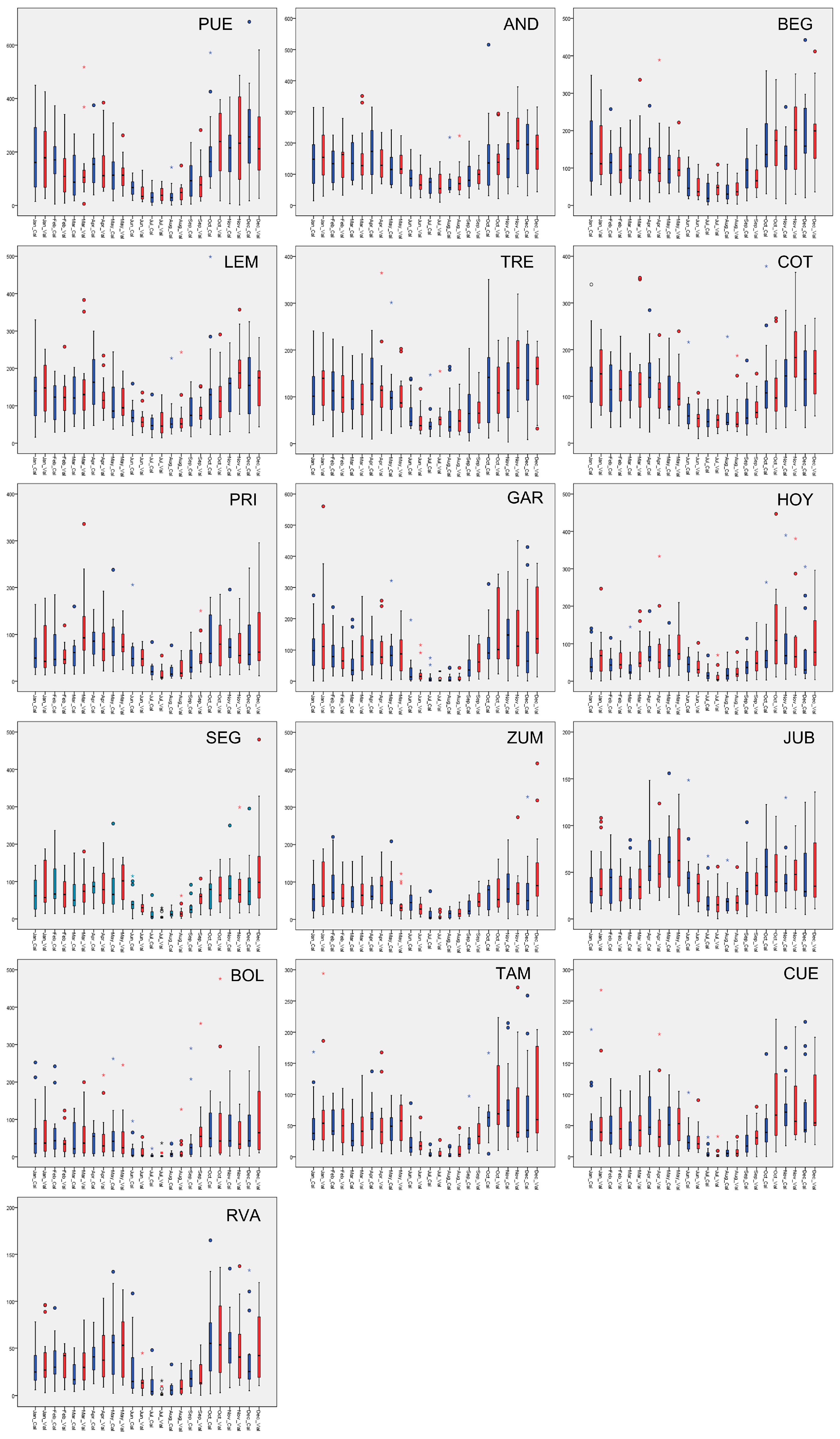
3.1. Precipitation Data Series Assessment

Firstly, we carried out an analysis of the monthly precipitation data series in Figure 3 using the boxplot graphics, distinguishing calibration (blue boxes) and validation (red boxes) periods, as the form of the evapotranspiration equation has limited influence on model performance in monthly hydrological models [147]. As can be seen in Figure 3, patterns of precipitation series in both periods are usually different, especially during the rainiest months that occur, mainly, from October to February in the more humid catchments (PUE, AND, BEG), thus decreasing (until May, even June) as the watershed becomes less humid (LEM, TRE, COT, PRI). The humid sub-humid ones (SEG, ZUM, JUB) shifted the rainiest period to spring, although maximums were also reached in winter. When the watershed is more arid, the distribution of precipitation over the year is more irregular, reaching similar values in December and June (RVA). This heterogeneity, not only between regions but also within the same watershed in both calibration and validation periods, represents different conditions and behaviors, which provides an optimal framework for hydrological purposes [87]. The driest period for all the watersheds occurs in summer months reaching, obviously, the lowest values in semi-arid and dry sub-humid watersheds. Likewise, July and August show the lowest variations, and consequently, the smallest boxplots. On the contrary, the highest differences are shown in the rainy months, varying in a wide range, reaching up to three times the median precipitation in nearly all watersheds. Concerning outliers in precipitation values (points and asterisks in Figure 3), the most humid watersheds, with aridity indices above 2 (PUE, AND, BEG), do not usually show numerous cases outside the bounds of the boxplots compared with the rest of the studied watersheds. When the aridity index ranges between 1 and 2, the monthly outliers in the boxplots occur more often and they are especially far out in the late spring or at the beginning of autumn. This trend levels out in humid sub-humid watersheds but dry sub-humid and semi-arid regions show extreme values for practically the whole year.

3.2. Models’ Parameters

Table 3 shows the main characteristics of the models’ structure, besides the range of parameters to be calibrated and the optimal ones found in the models and watersheds studied. Nearly all the optimal parameters of the models vary over the entire possible range. This circumstance is probably caused by the adaptation of the different hydrological processes embedded in the models’ structure to the wide diversity of the climatic conditions in the regions analyzed. Parameters related to storage capacity of the superficial tanks (H in Témez; a in GR2M; φ in Thornthwaite-Mather; A1, A2, A3 in AWBM, etc.) have a strong decreasing value trend when the watershed is drier, due to the average soil moisture throughout the year and the specific climatic conditions of each watershed. The finding is further confirmed in other parameters, such as the maximum soil moisture included in the Guo-5p model in the S parameter, whose values are around 500–1000 mm in humid and sub-humid regions and drop out at 50–70 mm in the driest watersheds, but we found no tendency when PET is summed, as the ABCD model takes parameter b into account. However, underground storage is only regionally sensitive when the aquifer capacity is important, regardless of the climatic location. Moreover, the ABCD model fails to perform the groundwater processes in semi-arid regions (d = 0), which is of high importance in the watersheds’ hydrological water balance. No correlations were found between the parameters and catchment area.

3.3. Goodness-of-Fit Tests

For a better understanding of the research and subsequent discussion, we ranked the results in tables and figures according to the AIU values.

3.3.1. AIC and BIC Criteria

AIC and BIC criteria classify the best model when the value achieved is lower. Although they penalize the number of estimated parameters, neither of them provide priority to the Thornthwaite-Mather model in this study (Table 4 and Table 5), as it has the fewest parameters to be estimated compared to the others used. In fact, it achieves less value in either of the watersheds. Both AIC (Table 4) and BIC (Table 5) show better results globally when using GR2M, proving to be the best model in 12 of the 16 catchments for AIC and 8 of the 16 for BIC, both in humid and dry sub-humid catchments. Témez, widely used in Spain, achieves the best result only in CUE for AIC and BIC, as well as for LEM and PRI, located in humid sub-humid areas. AWBM and Guo-5p reach the lowest values in humid sub-humid HOY, SEG, and ZUM. Focusing on the coefficient of variation (C.V.) in the last column of Table 4 and Table 5, it is clear that when the watershed is less humid, the C.V. obtained is higher, which means a clear difference between the used models. When AIU is higher than 1.5, the C.V. is below 10% but in the LEM watershed, the cover land changes are highlighted, for both AIC and BIC. Such minor differences indicate the similar performance of nearly all models studied in the most humid catchments. Nonetheless, if AIU is below 1.5, the C.V. becomes greater, which means a huge difference between the results achieved with the best model and with the rest of the models, reaching more than 130% in ZUM. Furthermore, in the driest watersheds, the C.V. is between 20% and 75%, which means that the AIC and BIC criteria are also the basis for the hydrological model selection in the dry and semi-arid ones, although the results may not differ in the humid ones.

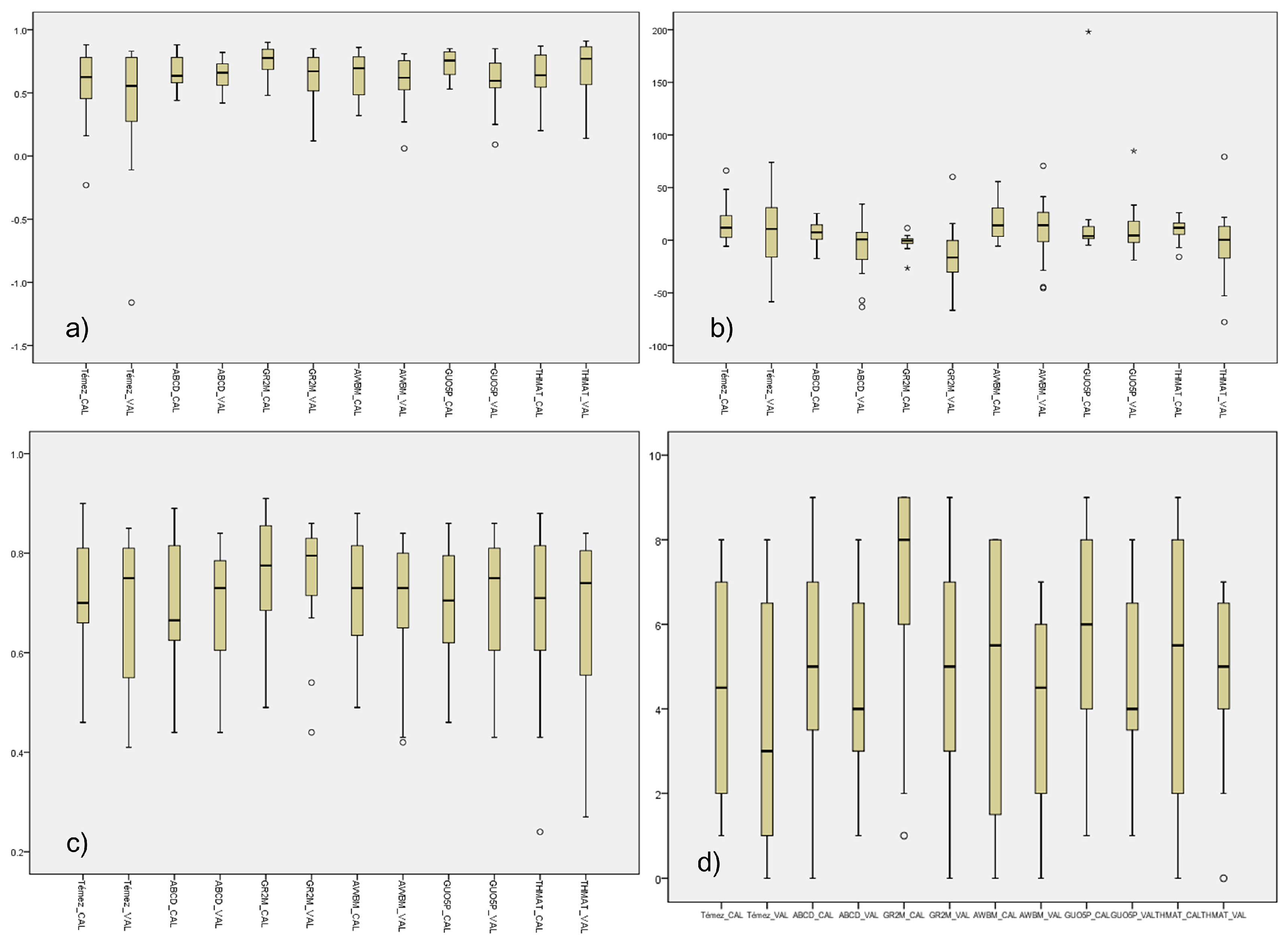
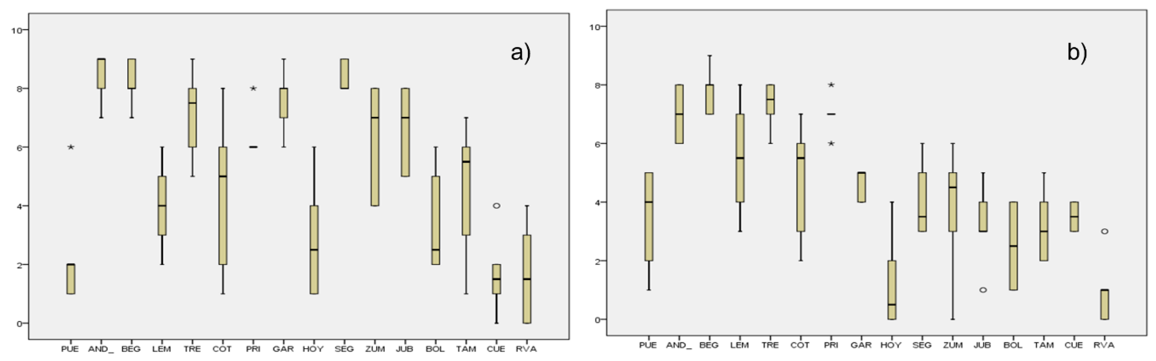
3.3.2. Grading Classification (NSE, PBIAS, R2)

In addition to the BIC and AIC criteria, we calculated NSE, PBIAS, and R2 and assessed a grading classification, according to Table 2, of the observed and simulated streamflow data (Qobs-Qsim) for all the evaluated approaches (Figure 4). The NSE for each model considering the 16 basins (Figure 4a) showed good results for all models except Témez, for which the average NSE (0.44) was below 0.50. Likewise, the most extreme outliers are shown for the Témez model in both the calibration and validation periods, reaching an absolute minimum below −1 in ZUM. AWBM and Guo-5p also show outliers in the validation period, although closer to the minimum values in respective boxplots, which correspond with the semi-arid watershed (RVA). GR2M and ABCD seem to be the best models, in general, in peninsular Spain according to the NSE values, although NSE for GR2M in semi-arid watersheds (RVA) is close to zero (0.18), and it is considered unsatisfactory. Despite being a five-parameter model, the Guo-5p would only be satisfactory according to the NSE criterion. However, a three-parameter model, such as the Thornthwaite-Mather, also achieved good results when considering only NSE (except in RVA), accounting for both wet and dry sub-humid Spain, which confirms the absence of the need for very complex water balance models, as suggested by Clark et al. [148], Perrin et al. [19], Jakeman and Hornberger [149], Michaud and Sorooshian [150], or Beven [151].
However, NSE cannot help identify model bias [124], and it should be complemented by other measures, such as PBIAS, in order to consider how well the model simulates the average magnitudes for the outputs and to identify the average model simulation bias (overprediction versus underprediction). The PBIAS boxplot for the models analyzed (Figure 4b) shows that this statistic technique provides an irregular rating of model performance without correlation with the aridity, as it provides high absolute values in the calibration and validation periods for all the models and watersheds. This may happen because PBIAS is very sensitive to extreme values [124] and its use is not particularly recommended to identify differences in the timing and magnitude of peak flows, such as in the case of the watersheds in peninsular Spain, as shown in the previous section. Notwithstanding, the best results are achieved with GR2M in calibration, but the validation period is more varied and ABCD and AWBM obtain similar results in PBIAS values.
Although the GR2M showed the best fit according R2 results, in nearly all catchments in the calibration (16 out of 16) and validation periods (14 out of 16), both semi-arid and sub-humid, we found an average correlation coefficient of close to 0.90. Boxplots for the rest of the models are not very different in either the median or amplitude (Figure 4a). The ABCD and AWBM models did not give the best fit in the validation period for any of the studied catchments, although their values were similar to those using the GR2M, especially for humid and sub-humid catchments. Increasing the number of parameters does not guarantee a better performance, as previous studies have shown [19,21,147,150,152], as the AWBM (6 parameters) did not show better results than the rest, even when it was compared to the lowest parameter model, the Thornthwaite-Mather (3 parameters), which had better results for nearly all watersheds, both humid and semi-arid. All water balance models showed correlation coefficients above 0.70 for humid and sub-humid catchments. In the dry sub-humid HOY and semi-arid RVA catchments, some values fell below 0.60, especially with the Thornthwaite-Mather and Témez models, despite the latter being widely used in Spain. It achieved the best fit only in the GAR and PRI catchments, taking similar values as the Guo-5p and GR2M coefficient. When the catchment was more arid, the R2 obtained was lower, which is in line with other studies [82,147]. It is essential to consider that R2 is oversensitive to extreme values [153] and insensitive to additive and proportional differences between model predictions and measured data [154], and it should be used with other goodness-of-fit tests and different criteria, both graphical and metrics, as we considered in this study, to provide consistency in the selection of models.
According to the grading classification criteria (Table 2) shown in Figure 4d, only the Témez model was unsatisfactory, whereas the rest were, on average, between good and satisfactory. This may be because the surpluses law of Témez is asymptotic to the one proposed by Thornthwaite-Mather for the highest precipitation values, but it differs on the lowest side of the curve, without requiring both the PET and soil moisture deficit to be used up completely. Furthermore, despite being a widely used hydrological model in Spain, underground Témez modeling is oversimplified and is invalid for karstic aquifers where there is more than one curve of discharge in the depletion of the aquifer [106].
With regards to the performance of the models’ results in each basin (Figure 5), we highlighted the influence of the aridity index, as mentioned before, which indicates that the climatic characteristics of the watershed are the most important issues in a model’s performance. When the watershed is drier, the worst performance is achieved, as the grading classification value decreases from humid to semi-arid regions. As might be expected, validation results (Figure 5a) are usually worse than the calibration ones (Figure 5b), reducing the range in the validation boxplots. However, PUE and LEM show better classification in the validation period, as there are more hydrological models whose NSE reach higher values than in calibration period. This may occur in cases where the measured data are bi-modal with high and low distributions in the same study area, such as the measured flows [155]. PRI is the only watershed that shows similar behavior to nearly all the models studied. Changes in land use in the last two decades (over 10% noticed in LEM and RVA) are not highlighted when using these metrics, especially in LEM, where the land use has changed almost 20% due to reforestation. Humid and humid sub-humid watersheds show good results in many of the hydrological models, with an average of 5–6 in the grading classification. This value decreases in dry sub-humid catchments until 4–2, and the semi-arid RVA only obtains satisfactory classification with GR2M in the calibration period and Guo5p in the validation period.
Table 6 summarizes the classification sum according to the grading criteria proposed in Table 2 for all studied catchments and models in both the calibration (1980–1995) and validation (1995–2010) periods. We selected the model that best fits each watershed according to the highest and similar values in the calibration and validation periods (Table 6). The GR2M gave the best fit of the catchments, with around 80% in the calibration period and 50% in the validation period with values over 7, meaning they all had a very good fit. The disparities between calibration and validation may be due to the climatic differences between the calibration and validation periods, as analyzed in previous sections. Semi-arid catchment, RVA, was unsatisfactory for the GR2M and for the rest of the models studied. These watersheds have a very irregular rainfall distribution, producing frequent run-off peaks, and although they have deep soil, low infiltration is produced; therefore, models do not achieve good results.
The Guo5p and Thornthwaite-Mather models were the best in the four catchments. The former has the best fit in some of the humid and humid sub-humid catchments but gives similar results to GR2M. However, Guo5p provides satisfactory results in dry sub-humid regions, whereas the rest of the models show important differences between calibration and validation periods. The ABCD model was the best in only one catchment but showed a value below 3 in the validation period, which means unsatisfactory. Nevertheless, humid watersheds show good behavior with nearly all the models, corroborating the better performance of nearly all models in wetter conditions. In general, the models that showed the best results on average, in all catchments, were first the GR2M, and then the Guo5p and Thornthwaite-Mather, with values around 7/5 (calibration/validation) for the GR2M model and around 5/5 (calibration/validation) for the Guo5p and Thornthwaite-Mather models. The AWBM and Témez showed the worst results, with 4/4 on average, which are almost unsatisfactory.
As with previous comparison methods, the best results were obtained in more humid basins, and the drier regions showed more unsatisfactory results. All of the analyses taken into account did not show a correlation between the catchment area and goodness-of-fit results, so higher model resolution does not seem to be an improvement for humid and sub-humid watersheds [74,156,157].

4. Discussion

4.1. Water Volume Assessment (REV)

The main aim of hydrological balance models is to assess inflows in a water resource system, and it is essential for appropriate analysis of its availability. Therefore, in addition to the assessment performed with the proposed grading classification (Table 2), we should analyze the differences between the total observed and simulated run-off volumes to validate or discard a model. Unlike the previous tests taken into account, REV results do not highlight one or two specific hydrological models, but the best fitted model for each catchment differs quite substantially. Table 7 shows the REV results of these comparisons for the catchments we studied and the models considered. According to this criterion, the Guo-5p and Thornwaite-Mather show the best results, on average, giving the best fitted models in three of the catchments studied. Témez is the worst model for nearly all catchments, reaching disparities that range between 10% and 80% compared to the best performances of other models. As with the BIC and AIC criteria, when the catchment is more arid, the differences between REV results are higher; therefore, there are several models that achieve REV lower than 10% for humid regions, provided that AIU is higher than 1.1. However, results for GR2M for LEM are higher, probably caused by the land cover change in the studied period. The worst results are shown in humid areas, with AIU around 1.0 and dry sub-humid and semi-arid catchments with REV around 20–40%, on average. REV is particularly unsatisfactory in semi-arid regions (RVA), where no model achieves values below 30%. Also noteworthy is the poor results shown by GR2M in dry sub-humid and semi-arid regions, which is in line with the classification of models in Table 6.

4.2. Model Selection

Table 8 shows the proposed model for each catchment, taking into account the proposed set of criteria: AIC, BIC, the grading method, and REV. Values of AIC and BIC in Table 8 denote the ranking position of the model according to these methods, varying between 1 and 6; 1 for the best result (lower value of the index) and 6 for the worst one. As seen in previous sections, the best results are achieved in humid regions for all the criteria taken into account. Furthermore, the AIC and BIC values match in most cases with the other used methods. We confirmed GR2M, as it was the best model in 50% of the catchments analyzed and had the best results in all of the goodness-of-fit tests applied. Moreover, it reached grades from good to very good according to Table 2, not only in humid catchments but also in humid sub-humid ones, with AIU being higher than 0.6 for ZUM and JUB. The good performance of GR2M may be due to its inclusion of a water exchange function alongside two independent parallel routing paths, which is of great importance in the transference between contrasting wet and dry periods [82]. Despite a value of AIU of 1.96 in LEM, only Témez is able to provide satisfactory results for all the criteria, with a REV lower than 10%. However, consideration should be made, as the land cover in LEM has changed more than 20% in the studied period.
Thornthwaite-Mather shows good performance in COT and SEG, although the AIC and BIC criteria do not classify this model as the best one, despite the low number of parameters. ABCD is considered unsatisfactory for HOY, but none of the remaining models obtained better results in this catchment. This may be caused by its altitude, as it is situated at around 1600 m, resulting in the highest altitude in our study, and snow precipitation events are relatively important and could affect hydrological modeling. Nonetheless, REV was below 10%, and the total volume assessment in the studied period can be considered good, although better results of REV (3.08) were achieved with Thornthwaite-Mather in HOY. Furthermore, the ABCD model enables surpluses, even when soil is not saturated, and the division between run-off and aquifer recharge is modeled by a constant time coefficient, which is rather unrealistic. Dry sub-humid and semi-arid catchments with AIU lower than 0.6 obtained the best performance with Guo5p, but results are unsatisfactory when AIU falls below 0.54, highlighting the relevance of aridity in lumped model performance. Regarding REV results, nearly all models show an error below 10%, although REV values increase to about 20% when the catchment is more arid. We did not find a trend for the catchment area or location and for the models used.

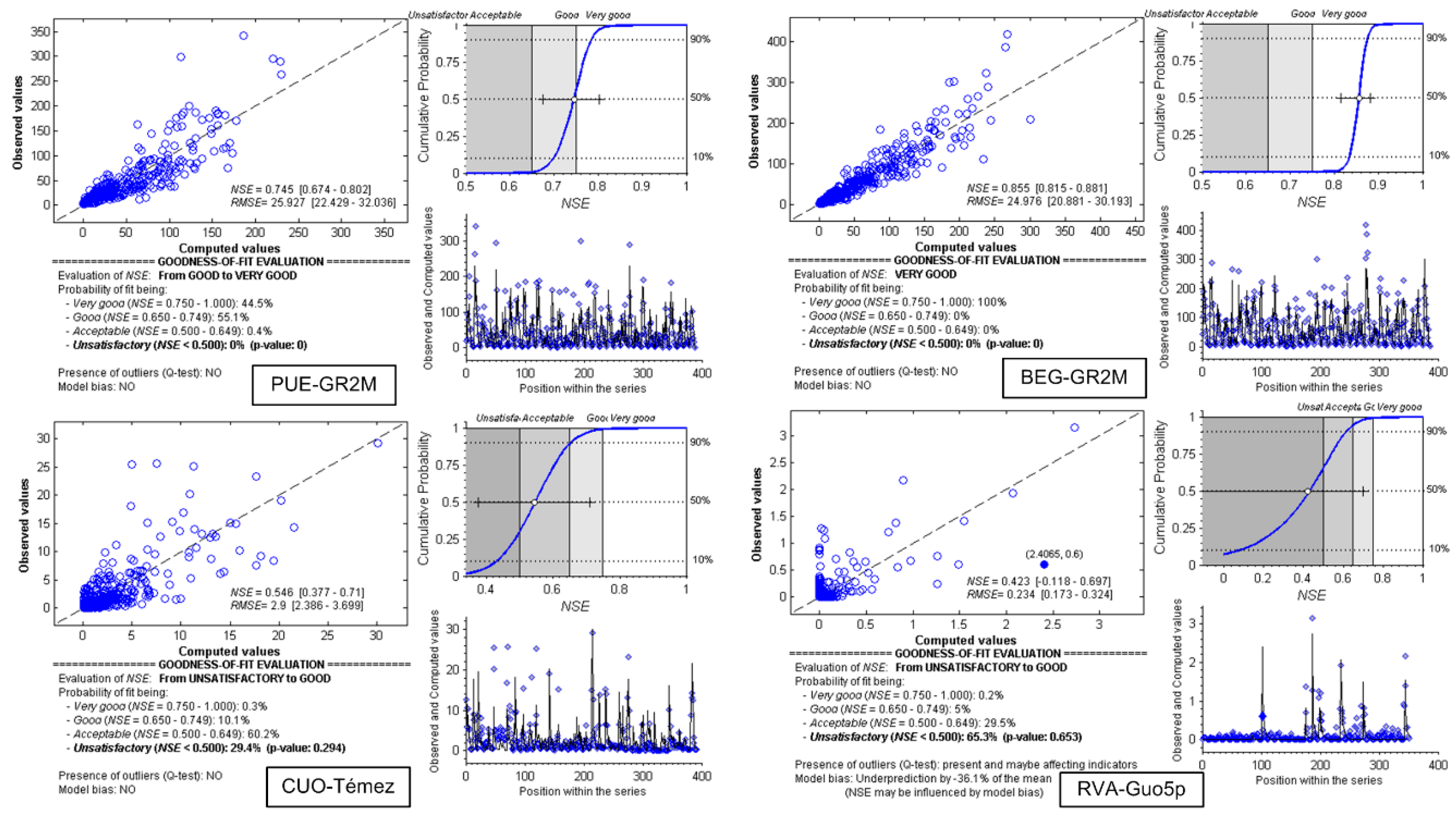
4.3. Models Uncertainty Analysis

After selecting the best model for each catchment in the studied period, defining the thresholds of acceptance of the model depends on its application of itself [158]. We used FITEVAL software [126] to provide an uncertainty framework of the results achieved. This application performs the goodness-of-fit of observed and simulated streamflows by the line balancing graphic versus line 1:1, the computation of NSE and RMSE and their corresponding values for the 95% confidence interval, the qualitative measure of adjustment, and the presence of bias and outliers. Figure 6 collects, as examples of FITEVAL, the outputs obtained for PUE, BEG, CUE, and RVA, and Table 9 shows the summary of results for each catchment and model selected in the previous sections. The values and graphics shown for GR2M models are by far the best compared to the rest of the models selected; therefore, more than 90% of the confidence intervals are above 0.75 NSE, considering that the model was very good in humid watersheds. When AIU was below 1.0, the confidence interval became greater for all the models, although GR2M also remained lower than the rest with an average range of 0.6–0.8 NSE, which means acceptable and very good models, respectively. On the contrary, Témez and Thornthwaite-Mather did not reach 0.75 NSE, even in humid catchments, and they fell by up to 0.1–0.3 NSE when AIU was below 1.0, such as SEG and CUE. Guo5p had similar performance in the most arid catchments and the confidence interval range comprises up to 70% of the uncertainty in the case of the semi-arid RVA. In general, outliers in catchments with AIU lower than 1.0 tend to underestimate the streamflow, whereas in the humid ones, the unusual presence of outliers tends to overestimate predictions around 5–10%.

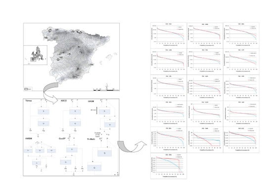
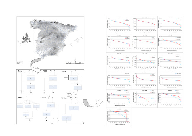
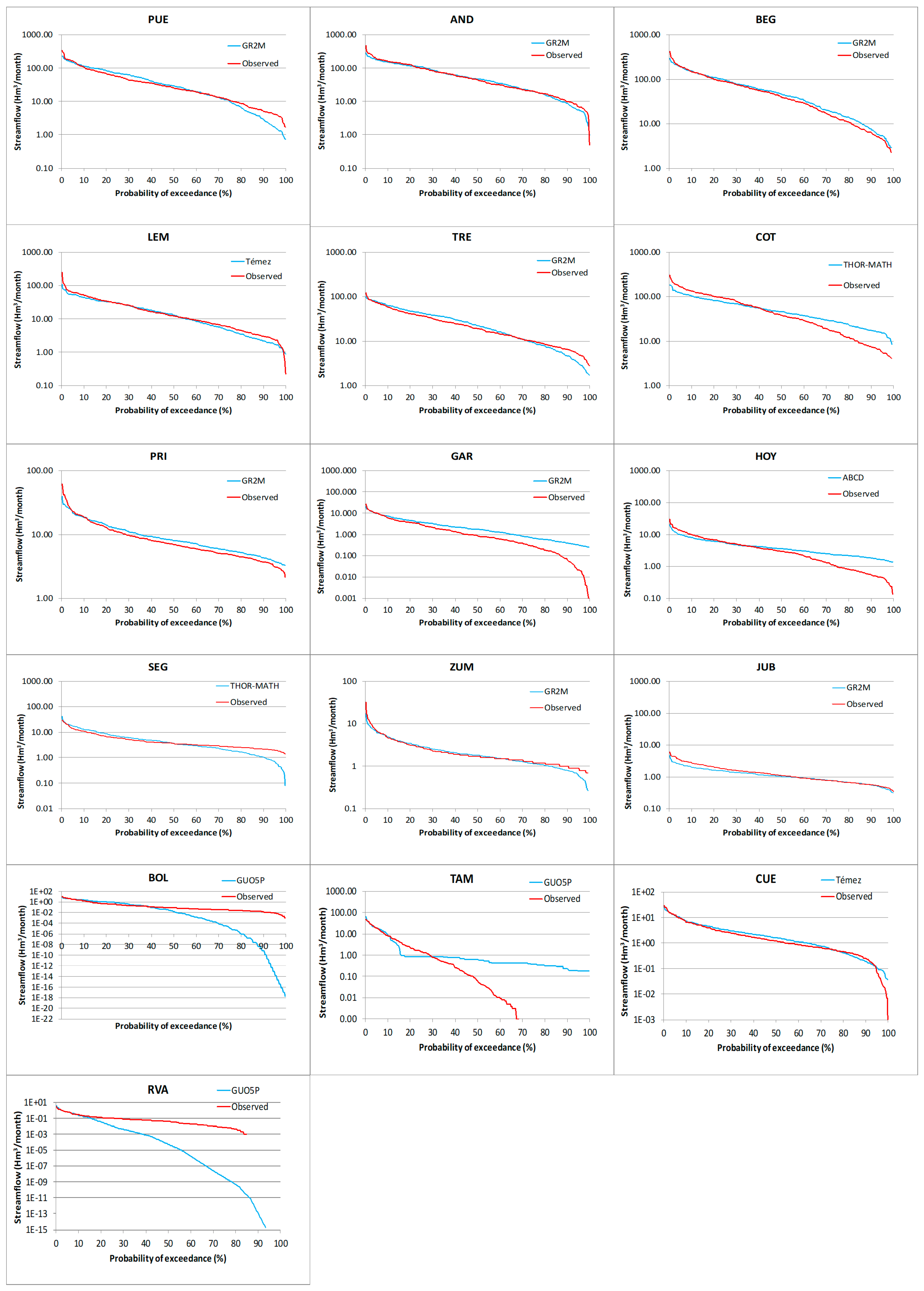
4.4. Flow Duration Curves

As our ultimate goal in this study is to use model predictions for the assessment of water availability, we developed FDCs for the observed and simulated streamflows for the whole studied period (1980–2010) (Figure 7) in order to evaluate the quality metrics related to different segments of the streamflow series. As previously determined, when the watershed is more humid, the best performance is obtained. All the watersheds had a similar pattern, in general terms, except the BOL, TAM, CUE, and RVA, which were the driest of those studied and were performed by the Guo5p and Témez models. However, Témez for LEM had good results, as REV suggested, although differences reached 59.4% in the low volumes. The graphics confirm the previous values of criteria and grading classification proposed, showing, in general, good performance in the highest and medium volumes. Lowest volumes had poor performance, especially when AIU was lower than 1. Concerning the humid and sub-humid regions, GR2M had good performance in probabilities of exceedance lower than 80%, (i.e., in high and medium volumes), but both curves were separated when the streamflow was lower. Thornthwaite-Mater’s model structure tends to underestimate low streamflow and to overestimate high streamflow, thus, even in COT with an AIU of 1.65, the observed and simulated FDCs are separated for high and low volumes. Table 10 quantifies the variabilities identified by FDCs using the signatures for high, low, and mid-segment volumes, as we described earlier. Deviations in humid and sub-humid watersheds ranged from 0–30% in both high volumes and mid-segment slopes, provided that GR2M was the model used. When AIU is below 1, the differences are significantly greater, regardless of the model, especially in the mid-segment and low-segment volume. Therefore, values in low volumes for humid watersheds showed an average of 30% but reached values higher than 100% when AIU was below 1, particularly marked in SEG, BOL, and RVA, which we performed using Guo5p and Thornthwaite-Mater. The best performance was obtained in the AND, BEG, and TRE watersheds (GR2M model), with values below 25% for all the signatures. Nonetheless, low volumes in most humid watersheds accounted for less than 5% of the total streamflow in the watersheds in the studied period, so their importance is relative for water resources assessment related to urban and agriculture water demand. Notwithstanding, as suggested by Operacz et al. [159] and Pusłowska-Tyszewska and Tyszewski [160], low flows have to be taken into account from an environmental point of view to maintain minimum ecological discharge. The differences in low volumes increased when the watershed was less humid. While high volumes’ differences stood at around 10–40%, signatures in low volumes reached negative 200–400%, overestimating streamflows in spring and summer seasons. As with humid regions, volumes with a probability of exceedance of 80% accounted for less than 8% of the total volume in the studied period. On the contrary, semi-arid regions showed good performance in high volumes, but both mid-segment slopes and low volumes had differences above 100% in most cases, and high volumes in these watersheds accounted for only 25% of the total streamflow in the studied period.

5. Conclusions

Spain has wide climate variation due to its complex orography and geographic situation. It has the driest and rainiest regions in continental Europe. Indeed, the 16 basins we selected as case studies cover a range of aridity index classifications from humid to semi-arid. We performed the assessment of the goodness-of-fit using various model selection criteria, so as to establish a robust methodology that can validate the conclusions obtained and its application in other different regions. Lumped hydrological balance models performed well in humid and sub-humid regions, regardless of the area, so higher model resolution does not seem to be an improvement for humid and sub-humid watersheds. The influence of the aridity index is highlighted in all of the goodness-of-fit tests carried out, which indicates that the climatic characteristics of the watershed are the most important issue in a model’s performance. When the watershed is more arid, the distribution of precipitation over the year is more irregular, and although these catchments have deep soil, low infiltration was produced; thus, the models did not achieve good results. Complexity in the models and over-parametrization do not guarantee a better performance, and three-parameters models, such as the Thornwaithe-Mather model, show, in some cases, better monthly simulations than the Guo-5p. However, although the driest regions registered “unsatisfactory” performance for the lumped models used and alternative methods (such as machine-learning modelling and semi-distributed models, such as SWAT [161]) will be assessed in future studies, the estimated run-off volumes with the Guo-5p are very similar to the observed ones, with differences below 12%, which is even lower than in some dry sub-humid regions.
The GR2M model gave the best fit in peninsular Spain. The performance indices proved satisfactory in both calibration and validation periods for most humid and sub-humid watersheds, so this model can be used for future water management in climate change scenarios and similar regions as the one studied, within an aridity index framework of around 1. When the catchment is more humid, any water model fits better. It is the opposite in the driest regions, thus, corroborating previous findings. The Témez model, widely used in Spain, only performed well in humid regions, as many of the other water balance models did, but it had the worst results in the dry sub-humid region. It only gave the best fit in the LEM and CUE, but the former showed a high C.V. in AIC and BIC, probably due to a 20% variation of cover land use in the studied period, and the latter had an unsatisfactory result for most of the tests applied.
It is clear that the use of a single comparison method is inaccurate, confusing, and in some cases, useless. When AIU is higher than 1.5, minor differences in AIC and BIC are found in the model performance; although they are also the basis for the hydrological model selection in the dry and semi-arid regions, these criteria must be used in conjunction with other methods to achieve the best model, especially in humid catchments. We used a grading method based on R2, NSE, and PBIAS that is complementary to AIC and BIC. Furthermore, the assessment of the margin of error in the total run-off volume using REV is also a key index. However, contrary to that observed in previous tests, the REV results do not highlight specific hydrological models, as well as the criteria above, if they are separately accounted for. These results indicate that it is not adequate to rely on a single hydrological model; also, the choice depends on the purpose of the studies. The uncertainty analysis carried out using the Fiteval software shows that the GR2M model is the best compared to the rest of the models selected; therefore, more than 90% of the confidence intervals are above 0.75 NSE, which shows that the model is very good in humid watersheds. On the contrary, Témez and Thornthwaite-Mather do not reach 0.75 NSE, even in humid catchments
FDCs and their metrics confirm previous results, as the humid and sub-humid region models show good performance in probabilities of exceedance lower than 80% (i.e., in high and medium volumes) but the results worsen the lower the streamflow is. Deviations in humid watersheds range from 0–25% in both high volumes and the mid-segment slope but reach values higher than 80% in low streamflows. Nonetheless, low volumes in most humid watersheds account for less than 5% of the total streamflow in the watersheds, so inaccuracy is admissible to the assessment of interannual water volume purposes. On the contrary, semi-arid regions show good performance in high volumes, which account for only 25% of the total streamflows in the studied period, thus disabling the models selected.
The methodology used can be applied in regions with similar case studies to more accurately assess the resources within a system and provide more sustainable management in a watershed.

Author Contributions

J.P.-S. and J.S.-A. conceived and designed the experiments. F.S.-M. performed the experiments and analyzed the data. D.P.-V. and R.S. provided reviews and suggestions. J.P.-S. and J.S.-A. prepared the manuscript with contributions from all co-authors.

Funding

This research received no external funding.

Acknowledgments

The authors acknowledge Papercheck Proofreading and Editing Services.

Conflicts of Interest

The authors declare no conflict of interest.

Appendix A. Témez Model

This model considers the system to be divided into the upper or non-saturated zone (S), and the lower or saturated zone (G). Some of the precipitation (P) drains directly into the river or through the aquifer, whereas the remainder is converted into ET (real evapotranspiration). Excess (Ex) is divided into run-off (Qs) through river networks at the present time, and infiltration to aquifers, draining one part (Qg) at the present time (month 0), with the rest remaining in the groundwater storage tank (G) for draining at a later date (month i).
Water balance is formed by input flow (P), which is divided into outflow (ET, Qs, and Qg), infiltration in month i (Ii), which is similar to aquifer recharge (Ri), and water storages in soil moisture (Si) and aquifer volume (Vi).
Total excess (Ex) in month i is obtained by Equations (A1)–(A3).
Ex i = 0   if   Pi P 0
Ex i = ( P i P 0 ) 2 P i + δ 2 P 0   if   Pi > P 0
δ = S max S i 1 + ET i
P 0 = C ( S max S i 1 )
where Smax is the soil maximum moisture (mm), Si-1, is the soil moisture (mm) at the beginning of the period i, ETPi is the potential evapotranspiration in the period I, and C is the beginning exceeding coefficient whose range is between 0.2 and 1. Soil moisture at the end of month i is obtained with Equation (A4).
S i = max ( 0 ; S i 1 + P i Ex i ETP i )
Moreover, ETi is obtained by Equation (A5) and Ii by Equation (A6).
ET i = min ( S i 1 + P i Ex i ;   ETP i )
I i = I max Ex i Ex i + I max
Run-off will be calculated as the excess that is not infiltrated, as in Equation (A7).
Qs i = Ex i I i
With respect to the aquifer, two hypotheses are made: (1) It behaves as a lineal water storage (Equation (A8)); and (2) the recharge by infiltration occurs in the middle of the period.
Q i = Q i l · e · t
where Qi is the outflow in time i, α is the aquifer discharge coefficient and t is the time period between i-l and i (Equation (A9)). The hypothesis of lineal water storage implies a relationship between Qi and stored volume in aquifer (Gi) given by Equation (A10).
Q i = ( Q i l · e · t / 2 + · R i ) e t / 2
Q i = α · G i
When applying mass balance equation (Equation (A11)) and combining with previous expressions, Equation (A12) is obtained.
I i Q i = dG i dEx
R i α · Gi = dG i dExi
Aquifer recharge can be expressed as Equation (A13).
R i = Sur I i
where Sur is the basin area.
Finally, Equation (A14) is used to calculate the stored water in the aquifer in month t, Equation (A15) provides aquifer drainage outflow, and total run-off in the monitoring point is obtained by Equation (A16).
G i = G i 1 e α t / 2 + Sur Ii α ( 1 e α t / 2 )
Qg i = V i 1 V i + R i
Q i = Qs i + Qg i

Appendix B. ABCD Model

This model (A, B, C, and D parameters) also considers two storage tanks, namely the upper storage (S) or soil tank, and the groundwater storage tank (G). The upper storage tank (S) has two outputs: run-off (Qs) and infiltration. Thus, the model has two inputs, precipitation (P) and ET, and their outputs are soil moisture content at the end of the month (S), monthly available water (W), ET, run-off (Qs), infiltration (I), groundwater run-off (Qb), monthly groundwater storage (G), and total run-off (Q).
The first step in the model consists of assessing the soil moisture at the end of the month (Si), using Equations (A17)–(A20).
W I = P i + S i 1
Yi = Wi + b 2 a ( Wi + b 2 a ) 2 Wi b a
I = Y i e ETP b
EI i = Y i S i
The second step is obtaining run-off (Qs) using Equation (A21).
Qs = ( 1 c ) ( W i Y i )
Groundwater run-off is obtained using Equations (A22)–(A24).
I = c ( W i Y i )
G i = ( I i + G i 1 ) ( 1 + d )
I = d G i
Finally, total run-off is calculated by adding the surface run-off and groundwater run-off (Equation (A25)).
Q i = Qs i + Qg i

Appendix C. GR2M

GR2M transforms precipitation into run-off through the implementation of two equations: production and transfer functions. Initially, P and ET are balanced and precipitation is distributed between the upper storage tank (S), with a limited capacity and groundwater storage tank (G).
Monthly P and ET are fitted using Equations (A26)–(A30).
U = P · ET ( R 0.5 + E 0.5 ) 2
P n = P U
ET n = ET U
P np = x 1 · P n
ET np = x 1 · ET n
where X1 is one parameter of the model.
Stored moisture in S tank is obtained when using Equation (A31).
S 1 = S + A · V 1 + S V A
where V = tan h ( P np A ) and A are the maximum storage capacity of tank S.
Likewise, ET causes S1 to become S2 when using Equation (A32).
S 2 = S 1 ( 1 W ) 1 + W ( 1 S 1 A )
Rainfall excess is calculated by Equation (A33).
Ex = P np + S S 1
Then, run-off (Qs) is obtained by Equation (A34).
Q s = α P e
where α is a parameter of the model.
Stored mositure in the second tank G (G1 y G2) receives a recharge of ( 1 α ) P e where G (initial stored in the tank) becomes G1, according to Equation (A35).
G 1 = G + ( 1 α ) P e
Groundwater run-off (Qg) is obtained by Equation (A36).
Q g = x 2 G 1
where X2 is another parameter of the model.
Finally, stored moisture in the second tank goes from G1 to G2 according to Equation (A37), and monthly total run-off is obtained by Equation (A38).
G 2 = G 1 Q s
Q = Q s + Q g

Appendix D. AWBM

This model has three surface water-storage tanks (S1, S2, and S3). The water balance of each is estimated independently, resulting in three surpluses. One part of these surpluses is transformed into run-off (Qs), and the other part percolates to a groundwater storage tank or aquifer (G), which in turn goes to groundwater run-off (Qg). Total flow (Q) is obtained by adding both run-offs.
The maximum capacity of each storage is obtained by Equation (A39).
S 1 = C ave 0.01 A 1 S 2 = C ave 0.33 A 2 S 3 = C ave 0.66 A 3
where Cave is the average soil water capacity and A1, A2, and A3 are the area of each tank.
For each tank P, ET, Ex, I, and total run-off (Q) are calculated according to Equations (A40)–(A43).
P k = A k P
ET k = min ( S k + P k ; A k ETP )
Ex k = max ( 0 ; S k + P k ET k Cap k )
S k = So k + P k ETR k Ex k
where k = 1, 2, and 3, Sok is the initial volume in each tank, and Ak the area of each tank. Run-off (Qs) is obtained using the fraction of total run-off corresponding to the base flow (BFI), using Equations (A44) and (A45).
Qs = ( 1 BFI ) · ( Ex 1 + Ex 2 + Ex 3 )
Ex = ( Ex 1 + Ex 2 + Ex 3 ) · BFI
Then, groundwater run-off is obtained by Equations (A46) and (A47).
Qg = Go K b
Qg a q u i f e r = G 0 + Ex Qg
where Kb is the recession constant.
Finally, total flow is obtained by adding both run-off from surface (Esup) and groundwater (Eaquifer) tanks (Equation (A48)).
Q total = Q S + Qg aquifer

Appendix E. Guo-5P

This model has a similar performance to the two-parameter Guo model, and its use is particularly recommended in humid and semi-humid regions. Precipitation and evapotranspiration (P and ET) are the input data, on the basis of which the remaining parameters are estimated: ET, soil water storage (S), water surpluses, surface run-off (Qs), subsurface run-off (Qb), aquifer recharge, groundwater storage (G), groundwater run-off (Qg), and total flow (Q).
Real ET is calculated by Equation (A49).
ETR i = ET i K 0
where K0 is a parameter of the model.
Soil water storage (Si) is limited by soil maximum moisture (SMAX), which is obtained when using Equations (A50) and (A51)
If   Pi > ETRi   then   S i = S i 1 + P i ETR i
If   Pi < ETRi   then   S i = S i 1 e ( ETR Pi ) SMAX
When P is higher than ET and soil moisture reaches its maximum (SMAX), water excess (Exi) is obtained by Equation (A52).
Ex i = S i SMAX
Part of the water excess becomes run-off (QSi), whereas the rest of the water excess (WSi) is divided between subsurface run-off (Qsi) and infiltration (Ii) according to Equations (A53)–(A56).
Q si = C · ( S i SMAX ) = C · Ex
WS i = ( 1 C ) · ( S i SMAX ) = ( 1 C ) · Ex
QI i = K 1 · WS i
I i = ( 1 K 1 ) · WS i
where C and K1 are parameters of the model and QIi is the sub-superficial run-off.
The model considers that aquifer balance is obtained when using Equation (A57).
G i = G i 1 + I i K 2 G i 1
where K2 is a parameter of the model.
The underground run-off (Qg) is calculated by Equation (A58).
Qg i = K 2 G i
Finally, total run-off (Q) is assessed adding run-off, sub-superficial run-off, and underground run-off (Equation (A59)).
Q = Q si + QI i + Qg i 1

Appendix F. Thornthwaite-Mather

The model distinguishes two water storage tanks—surface (S) and groundwater (G)—which lead to the output flow (Q) through different calculations.
A part of P is converted into run-off (Qd) directly (Equation (A60)).
Qd = P
The remaining precipitation that comes into the model (Pi) is compared to ET, obtaining soil moisture capacity (S). If Pi is higher than ET, then there is water excess and real evapotranspiration (ETR), and final storage (Si) is obtained by Equation (A61), and is otherwise obtained using Equation (A62).
S i = min ( S i 1 + P i ETP ) ; )
ET i = S i 1 S + P i
Thus, if surface storage (S) is full, flow to the tank is calculated by Equation (A63), and is otherwise obtained with ΔQ = 0.
Δ Q = P i ETP i + S i 1
Finally, only one part of the available water in an underground water tank (G) will be added to total run-off (Q), which will be obtained by Equation (A64).
G i = Q ( 1 λ )
where λ is a parameter of the model.
Therefore, Q is obtained by adding direct and underground run-off (Equation (A65)).
Q t = Qd + Qg

References

  1. Wurbs, R.A. Texas water availability modeling system. J. Water Resour. Plan. Manag. 2005, 131, 270–279. [Google Scholar] [CrossRef]
  2. Senent-Aparicio, J.; Liu, S.; Pérez-Sánchez, J.; López-Ballesteros, A.; Jimeno-Sáez, P. Assessing Impacts of Climate Variability and Reforestation Activities on Water Resources in the Headwaters of the Segura River Basin (SE Spain). Sustainability 2018, 10, 3277. [Google Scholar] [CrossRef]
  3. Puricelli, M.M. Estimación y Distribución de Parámetros del Suelo Para la Modelación Hidrológica. Ph.D. Thesis, Departamento de Ingeniería Hidráulica y Medio Ambiente, Universidad Politécnica de Valencia, Valencia, Spain, 2003. [Google Scholar]
  4. Essam, M. Water Flow and Chemical Transport in a Subsurface Drained Watershed. Ph.D. Thesis, University of Illinois, Champaign County, IL, USA, 2007. [Google Scholar]
  5. Shimon, C. Water Resources; Island Press: Washington, DC, USA, 2010. [Google Scholar]
  6. Unesco. Methods for Water Balance Computation; Instituto de Hidrología de España: Madrid, Spain, 1981. [Google Scholar]
  7. Thornthwaite, C.W. A new and improved classification of climates. Geogr. Rev. 1948, 38, 55–94. [Google Scholar] [CrossRef]
  8. Thornthwaite, C.W.; Mather, J.R. Instructions and Tables for Computing Potential Evapotranspiration and the Water Balance; Publications in Climatology; Drexel Institute of Technology, Laboratory of Climatolog: Centerton, NJ, USA, 1957; Volume 10. [Google Scholar]
  9. Alley, W.M. On the treatment of evapotranspiration, soil moisture accounting, and aquifer recharge in monthly water balance models. Water Resour. Res. 1984, 20, 1137–1149. [Google Scholar] [CrossRef]
  10. Xiong, L.; Guo, S. A two-parameter monthly water balance model and its application. J. Hydrol. 1999, 216, 111–123. [Google Scholar] [CrossRef]
  11. Makhlouf, Z.; Michel, C. A two-parameter monthly water balance model for French watersheds. J. Hydrol. 1994, 162, 299–318. [Google Scholar] [CrossRef]
  12. Giakoumakis, S.; Tsakiris, G.; Efremides, D. On the Rainfall-Run-Off Modelling in a Mediterranean Island Environment; Advances in Water Resources Technology; Tsakiris, G., Ed.; Balkema: Rotterdam, The Netherlands, 1991. [Google Scholar]
  13. Mimikou, M.A.; Hadjisawa, P.S.; Kouvopoulos, Y.S.; Afrateos, H. Regional climate change impacts: II. Impacts on water management works. Hydrol. Sci. J. 1991, 36, 259–270. [Google Scholar] [CrossRef]
  14. Alley, W.M. Water balance models in one-month-ahead streamflow forecasting. Water Resour. Res. 1985, 21, 597–606. [Google Scholar] [CrossRef]
  15. Abulohom, M.S.; Shah, S.M.S.; Ghumman, A.R. Development of a rainfall-run-off model, its calibration and validation. Water Resour. Manag. 2001, 15, 149–163. [Google Scholar] [CrossRef]
  16. Yates, D.; Strzepek, K. Modeling the Nile basin under climate change. J. Hydrol. Eng. 1998, 3, 98–108. [Google Scholar] [CrossRef]
  17. Vandewiele, G.; Xu, C.-Y. Methodology and comparative study of monthly water balance models in Belgium, China and Burma. J. Hydrol. 1992, 134, 315–347. [Google Scholar] [CrossRef]
  18. Andréassian, V.; Hall, A.; Chahinian, N.; Schaake, J. Introduction and Synthesis: Why Should Hydrologists Work on A Large Number of Basin Data Sets? In Large Sample Basin Experiments for hydrological Model Parameterization, Results of the Model Parameter Experiment—MOPEX; IAHS Publication No. 307; IAHS Press: Paris, France, 2006. [Google Scholar]
  19. Perrin, C.; Michel, C.; Andreassian, V. Does a large number of parameters enhance model performance? Comparative assessment of common catchment model structures on 429 catchments. J. Hydrol. 2001, 242, 275–301. [Google Scholar] [CrossRef]
  20. Chiew, F.H.S.; McMahon, T.A. Australian Data for Rainfall-Run-Off Modelling and the Calibration of Models Against Streamflow Data Recorded Over Different Time Periods; Civil Engineering Transactions, The Institution of Engineers: Sydney, Australia, 1993; Volume 35, pp. 261–274. [Google Scholar]
  21. World Meteorological Organization. Intercomparison of Conceptual Models Used in Operational Forecasting; Operational Hydrology Report No. 7, WMO-No. 429; WMO: Geneva, Switzerland, 1975. [Google Scholar]
  22. Xu, C.Y.; Singh, V.P. Dependence of evaporation on meteorological variables at different time-scales and intercomparison of estimation methods. Hydrol. Process. 1998, 12, 429–442. [Google Scholar] [CrossRef]
  23. Todini, E. Rainfall-runoff modeling—past present and future. J. Hydrol. 1998, 100, 341–352. [Google Scholar] [CrossRef]
  24. Chiew, F.H.S.; Kirono, D.G.C.; Kent, D.M.; Frost, A.J.; Charles, S.P.; Timbal, B.; Nguyen, K.C.; Fu, G. Comparison of run-off modelled using rainfall from different downscaling methods for historical and future climates. J. Hydrol. 2010, 387, 10–23. [Google Scholar] [CrossRef]
  25. Zhang, Q.; Liu, J.; Singh, V.P.; Gu, X.; Chen, X. Evaluation of impacts of climate change and human activities on streamflow in the Poyang Lake basin, China. Hydrol. Process. 2016, 30, 2562–2576. [Google Scholar] [CrossRef]
  26. Wang, D.; Tang, Y. A one-parameter Budyko model for water balance captures emergent behavior in Darwinian hydrologic models. Geophys. Res. Lett. 2014, 41, 4569–4577. [Google Scholar] [CrossRef]
  27. Sankarasubramanian, A.; Vogel, R.M. Annual hydroclimatology of the United States. Water Resour. Res. 2002, 38, 19-1–19-2. [Google Scholar] [CrossRef]
  28. Lacombe, G.; Ribolzi, O.; De Rouw, A.; Pierret, A.; Latsachak, K.; Silvera, N.; Dinh, R.P.; Orange, D.; Janeau, J.L.; Soulileuth, B.; et al. Contradictory hydrological impacts of afforestation in the humid tropics evidenced by long-term field monitoring and simulation modelling. Hydrol. Earth Syst. Sci. 2016, 20, 2691–2704. [Google Scholar] [CrossRef]
  29. Mouelhi, S.; Michel, C.; Perrin, C.; Andreassian, V. Stepwise development of a two parameter monthly water balance model. J. Hydrol. 2006, 318, 200–214. [Google Scholar] [CrossRef]
  30. Burnash, R.J.C.; Ferral, R.L.; Maguire, R.A. A Generalized Streamflow Simulation System: Conceptual Models for Digital Computers; Joint Federal State River Forecast Center: Sacramento, CA, USA, 1973.
  31. Guo, S. Impact of Climate Change on Hydrological Balance and Water Resource Systems in the Dongjiang Basin, China; Modeling and Management of Sustainable Basin-Scale Water Resource Systems (Proceedings of a Boulder Symposium); LAHS Publ.: Los Alamos, NM, USA, 1995; Volume 231. [Google Scholar]
  32. Singh, K.; Kumar, A. Evaluation of relief aspects morphometric parameters derived from different sources of DEMs and its effects over time of concentration of run-off (TC). Earth Sci. Inform. 2016. [Google Scholar] [CrossRef]
  33. Singh, S.K. Transmuting synthetic unit hydrograph into gamma distribution. J. Hydrol. Eng. 2000, 5, 380–385. [Google Scholar] [CrossRef]
  34. Ferrer, J. Recomendaciones para el Cálculo Hidrometeorológico de Avenidas; CEDEX M-37, CEDEX: Madrid, Spain, 1993. [Google Scholar]
  35. Témez, J.R. Extended and Improved Rational Method: Version of the Highways Administration of Spain. In Proceedings of the XXIV Congress of IAHR, Madrid, Spain, 9–13 September 1991; Volume A, pp. 33–40. [Google Scholar]
  36. Témez, J.R. Cálculo Hidrometeorológico de Caudales Máximos en Pequeñas Cuencas Naturales; Dirección General de Carreteras, MOPU: Madrid, Spain, 1987.
  37. Lyon, S.W.; Walter, M.T.; Gerard-Marchant, P.; Steenhuis, T.S. Using a topographic index to distribute variable source area run-off predicted with the SCS curve-number equation. Hydrol. Proc. 2004, 18, 2757–2771. [Google Scholar] [CrossRef]
  38. Frankenberger, J.R.; Brooks, E.S.; Walter, M.T.; Walter, M.F.; Steenhuis, T.S. A GIS-Based Variable Source Area Hydrology Model. Hydrol. Process. 1999, 13, 804–822. [Google Scholar] [CrossRef]
  39. Calvo, J.C. An evaluation of Thornthwaite’s water balance technique in predicting stream run-off in Costa Rica. Hydrol. Sci. J. 1986, 31, 51–60. [Google Scholar] [CrossRef]
  40. Croke, B.F.W.; Andrews, F.; Jakeman, A.J.; Cuddy, S.M.; Luddy, A. IHACRES classic plus: A redesign of the IHACRES rainfall-run-off model. Environ. Model. Softw. 2006, 21, 426–427. [Google Scholar] [CrossRef]
  41. Chiew, F.H.S.; McMahon, T.A. Modelling the impacts of climate change on Australian streamflow. Hydrol. Process. 2002, 16, 1235–1245. [Google Scholar] [CrossRef]
  42. Perrin, C.; Michel, C.; Andréassian, V. Improvement of a parsimonious model for streamflow simulation. J. Hydrol. 2003, 279, 275–289. [Google Scholar] [CrossRef]
  43. Boughton, W. New approach to calibration of the AWBM for use on ungauged catchments. J. Hydrol. Eng. 2009, 14, 562–568. [Google Scholar] [CrossRef]
  44. Boughton, W. Effect of data length on rainfall–run-off modelling. Environ. Model. Softw. 2007, 22, 406–413. [Google Scholar] [CrossRef]
  45. Boughton, W. Calibrations of a daily rainfall–run-off model with poor quality data. Environ. Model. Softw. 2006, 21, 1114–1128. [Google Scholar] [CrossRef]
  46. Boughton, W. The Australian Water Balance Model. Environ. Model. Softw. 2004, 19, 943–956. [Google Scholar] [CrossRef]
  47. Boughton, W.; Chiew, F. Estimating run-off in ungauged catchments from rainfall, PET and the AWBM model. Environ. Model. Softw. 2007, 22, 476–487. [Google Scholar] [CrossRef]
  48. O’Connell, P.E.; Nash, J.E.; Farrell, J.P. River flow forecasting through conceptual models, Part 2, The Brosna catchment at Ferbane. J. Hydrol. 1970, 10, 317–329. [Google Scholar] [CrossRef]
  49. Singh, V.P. Watershed Modeling. In Computer Models of Watershed Hydrology, 1st ed.; Water Resources Publications: Highlands Ranch, CO, USA, 1995. [Google Scholar]
  50. Singh, V.P.; Frevert, D.K. Mathematical Models of Small Watershed Hydrology and Applications; Water Resources Publications: Littleton, CO, USA, 2002. [Google Scholar]
  51. Eder, G.; Fuchs, M.; Nachtnebel, H.; Loibl, W. Semi-distributed modelling of the monthly water balance in an alpine catchment. Hydrol. Process. 2005, 19, 2339–2360. [Google Scholar] [CrossRef]
  52. Arnold, J.G.; Srinivasan, R.; Muttiah, R.S.; Williams, J.R. Large-area hydrologic modeling and assessment: Part I. Model development. J. Am. Water Resour. Assoc. 1998, 34, 73–89. [Google Scholar] [CrossRef]
  53. Beven, K.J. Rainfall-Run-off Modelling: The Primer; Wiley: Chichester, UK, 2001. [Google Scholar]
  54. Ewen, J.; Parkin, G. Validation of catchment models for prediction land use and climate change impact. 1. Method. J. Hydrol. 1996, 175, 583–594. [Google Scholar] [CrossRef]
  55. Carpenter, T.M. Discretization scale dependencies of the ensemble flow range versus catchment area relationship in distributed hydrologic modeling. J. Hydrol. 2006, 328, 242–257. [Google Scholar] [CrossRef]
  56. Viney, N.R.; Croke, B.F.W.; Breuer, L.; Bormann, H.; Bronstert, A.; Frede, H.; Gräff, T.; Hubrechts, L.; Huisman, J.A.; Jakeman, A.J.; et al. Ensemble modelling of the hydrological impacts of land use change. In Proceedings of the MODSIM05—International Congress on Modelling and Simulation: Advances and Applications for Management and Decision Making, Melbourne, Australia, 12–15 December 2005; Zerger, A., Argent, R.M., Eds.; ANU: Canberra, Australia, 2005; pp. 2967–2973. [Google Scholar]
  57. Croke, B.F.W.; Merritt, W.S.; Jakeman, A.J. A dynamic model for predicting hydrologic response to land cover changes in gauged and ungauged catchments. J. Hydrol. 2004, 291, 115–131. [Google Scholar] [CrossRef]
  58. Vansteenkiste, T.; Tavakoli, M.; Ntegeka, V.; De Smedt, F.; Batelaan, O.; Pereira, F.; Willems, P. Intercomparison of hydrological model structures and calibration approaches in climate scenario impact projections. J. Hydrol. 2014, 519, 743–755. [Google Scholar] [CrossRef]
  59. Samaniego, L.; Kumar, R.; Attinger, S. Multiscale parameter regionalization of a grid--based hydrologic model at the mesoscale. Water Resour. Res. 2010, 46, W05523. [Google Scholar] [CrossRef]
  60. Beck, H.E.; van Dijk, A.I.J.M.; de Roo, A.; Miralles, D.G.; McVicar, T.R.; Schellekens, J.; Bruijnzeel, L.A. Global-scale regionalization of hydrologic model parameters. Water Resour. Res. 2016, 52, 3599–3622. [Google Scholar] [CrossRef]
  61. Yang, X.; Michel, C. Flood forecasting with a watershed model: A new method of parameter updating. Hydrol. Sci. J. 2000, 45, 537–546. [Google Scholar] [CrossRef]
  62. Cameron, D.S.; Beven, K.J.; Tawn, J.; Blazkova, S.; Naden, P. Flood frequency estimation by continuous simulation for a gauged upland catchment (with uncertainty). J. Hydrol. 1999, 219, 169–187. [Google Scholar] [CrossRef]
  63. Uhlenbrock, S.; Seibert, J.; Leibundgut, C.; Rohde, A. Prediction uncertainty of conceptual rainfall-run-off models caused by problems in identifying model parameters and structure. Hydrol. Sci. J. 1999, 44, 779–797. [Google Scholar] [CrossRef]
  64. Yang, X.; Parent, E.; Michel, C.; Roche, P.A. Comparison of real-time reservoir operation techniques. J. Water Resour. Plan. Manag. 1995, 121, 345–351. [Google Scholar] [CrossRef]
  65. Lobligeois, F.; Andréassian, V.; Perrin, C.; Tabary, P.; Loumagne, C. When does higher spatial resolution rainfall information improve streamflow simulation? An evaluation on 3620 flood events. Hydrol. Earth Syst. Sci. 2013, 10, 12485–12536. [Google Scholar] [CrossRef]
  66. Smith, M.B.; Koren, V.; Zhang, Z.; Zhang, Y.; Reed, S.M.; Cui, Z.; Moreda, F.; Cosgrove, B.A.; Mizukami, N.; Anderson, E.A. Results of the DMIP 2 Oklahoma experiments. J. Hydrol. 2012, 418–419, 17–48. [Google Scholar] [CrossRef]
  67. Apip; Sayama, T.; Tachikawa, Y.; Takara, K. Spatial lumping of a distributed rainfall sediment-run-off model and its effective lumping scale. Hydrol. Process. 2012, 26, 855–871. [Google Scholar] [CrossRef]
  68. Breuer, L.; Huisman, J.A.; Willems, P.; Bormann, H.; Bronstert, A.; Croke, B.F.W.; Frede, H.-G.; Gräff, T.; Hubrechts, L.; Jakeman, A.J.; et al. Assessing the impact of land use change on hydrology by ensemble modeling (LUCHEM) I: Model intercomparison of current land use. Adv. Water Resour. 2009, 32, 129–146. [Google Scholar] [CrossRef]
  69. Zhang, Z.; Koren, V.; Smith, M.; Reed, S.; Wang, D. Use of next generation weather radar data and basin disaggregation to improve continuous hydrograph simulations. J. Hydrol. Eng. 2004, 9, 103–115. [Google Scholar] [CrossRef]
  70. Koren, V.; Reed, S.; Smith, M.; Zhang, Z.; Seo, D.J. Hydrology laboratory research modeling system (HL-RMS) of the US national weather service. J. Hydrol. 2004, 291, 297–318. [Google Scholar] [CrossRef]
  71. Ajami, N.K.; Gupta, H.; Wagener, T.; Sorooshian, S. Calibration of a semidistributed hydrologic model for streamflow estimation along a river system. J. Hydrol. 2004, 298, 112–135. [Google Scholar] [CrossRef]
  72. Reed, S.; Koren, V.; Smith, M.B.; Zhang, Z.; Moreda, F.; Seo, D.; Dmipparticipants, A. Overall distributed model intercomparison project results. J. Hydrol. 2004, 298, 27–60. [Google Scholar] [CrossRef]
  73. Boyle, D.P.; Gupta, H.V.; Sorooshian, S.; Koren, V.; Zhang, Z.; Smith, M. Toward improved streamflow forecasts: Value of semidistributed modeling. Water Resour. Res. 2001, 37, 2749–2759. [Google Scholar] [CrossRef]
  74. Refsgaard, J.C.; Knudsen, J. Operational validation and intercomparison of different types of hydrological models. Water Resour. Res. 1996, 32, 2189–2202. [Google Scholar] [CrossRef]
  75. Shah, S.M.S.; O’Connell, P.E.; Hosking, J.R.M. Modelling the effects of spatial variability in rainfall on catchment response. 2. Experiments with distributed and lumped models. J. Hydrol. 1996, 175, 89–111. [Google Scholar] [CrossRef]
  76. Bormann, H.; Breuer, L.; Giertz, S.; Huisman, J.A.; Viney, N.R. Spatially explicit versus lumped models in catchment hydrology—Experiences from two case studies. In Uncertainties in Environmental Modelling and Consequences for Policy Making. NATO Science for Peace and Security Series C: Environmental Security; Baveye, P.C., Laba, M., Mysiak, J., Eds.; Springer: Dordrecht, The Netherlands, 2009. [Google Scholar]
  77. Vansteenkiste, T.; Tavakoli, M.; Van Steenbergen, N.; De Smedt, F.; Batelaan, O.; Pereira, F.; Willems, P. Intercomparison of five lumped and distributed models for catchment run-off and extreme flow simulation. J. Hydrol. 2014, 511, 335–349. [Google Scholar] [CrossRef]
  78. Martínez-Santos, P.; Andreu, J.M. Lumped and distributed approaches to model natural recharge in semiarid karst aquifers. J. Hydrol. 2010, 388, 389–398. [Google Scholar] [CrossRef]
  79. Haque, M.M.; Rahman, A.; Hagare, D.; Kibria, G.; Karim, F. Estimation of catchment yield and associated uncertainties due to climate change in a mountainous catchment in Australia. Hydrol. Process. 2015, 29, 4339–4349. [Google Scholar] [CrossRef]
  80. Jiang, T.; Chen, Y.Q.; Xu, C.Y.; Chen, X.H.; Chen, X.; Singh, V.P. Comparison of hydrological impacts of climate change simulated by six hydrological models in the Dongjiang Basin, South China. J. Hydrol. 2007, 336, 316–333. [Google Scholar] [CrossRef]
  81. Kumar, A.; Singh, R.; Jena, P.P.; Chatterjee, C.; Mishra, A. Identification of the best multi-model combination for simulating river discharge. J. Hydrol. 2015, 525, 313–325. [Google Scholar] [CrossRef]
  82. Van Esse, W.R.; Perrin, C.; Booij, M.J.; Augustijn, D.C.M.; Fenicia, F.; Kavetski, D.; Lobligeois, F. The influence of conceptual model structure on model performance: A comparative study for 237 French catchments. Hydrol. Earth Syst. Sci. 2013, 17, 4227–4239. [Google Scholar] [CrossRef]
  83. Velázquez, J.A.; Anctil, F.; Perrin, C. Performance and reliability of multimodel hydrological ensemble simulations based on seventeen lumped models and a thousand catchments. Hydrol. Earth Syst. Sci. 2010, 14, 2303–2317. [Google Scholar] [CrossRef]
  84. Broderick, C.; Matthews, T.; Wilby, R.L.; Bastola, S.; Murphy, C. Transferability of hydrological models and ensemble averaging methods between contrasting climatic periods. Water Resour. Res. 2016, 52, 8343–8373. [Google Scholar] [CrossRef]
  85. Bourgin, F.; Andréassian, V.; Perrin, C.; Oudin, L. Transferring global uncertainty estimates from gauged to ungauged catchments. Hydrol. Earth Syst. Sci. 2015, 19, 2535–2546. [Google Scholar] [CrossRef]
  86. Ye, W.; Bates, B.; Viney, N.; Sivapalan, M.; Jakeman, A. Performance of conceptual rainfall-run-off, models in low-yielding ephemeral catchments. Water Resour. Res. 1997, 33, 153–166. [Google Scholar] [CrossRef]
  87. Kirchner, J.W. Getting the right answers for the right reasons: Linking measurements, analyses, and models to advance the science of hydrology. Water Resour. Res. 2006, 42, W03S04. [Google Scholar] [CrossRef]
  88. Escriva-Bou, A.; Pulido-Velazquez, M.; Pulido-Velazquez, D. Economic value of climate change adaptation strategies for water management in Spain’s Jucar basin. J. Water Res. Plan. ASCE 2017, 143, 04017005. [Google Scholar] [CrossRef]
  89. MIMAM, Libro Blanco del Agua en España; Centro de Publicaciones del Ministerio de Medio Ambiente: Madrid, Spain, 2000.
  90. Cabezas, F.; Estrada, F.; Estrela, T. Algunas contribuciones técnicas del Libro Blanco del Agua en España. Ingeniería Civil 1999, 115, 79–96. [Google Scholar]
  91. Estrela, T.; Cabezas, F.; Estrada, F. La evaluación de los recursos hídricos en el libro blanco del agua en España. Ingeniería del Agua 1999, 6, 125–138. [Google Scholar] [CrossRef]
  92. Estrela, T. Modelos Matemáticos para la Evaluación de Recursos Hídricos; Centro de Estudios Hidrográficos y Experimentación de Obras Públicas, CEDEX: Madrid, Spain, 1992. [Google Scholar]
  93. Fernandez, W.; Vogel, R.; Sankarasubramanian, A. Regional calibration of a watershed model. Hydrol. Sci. J. 2000, 45, 689–707. [Google Scholar] [CrossRef]
  94. Martinez, G.F.; Gupta, H.V. Toward improved identification of hydrological models: A diagnostic evaluation of the “abcd” monthly water balance model for the conterminous United States. Water Resour. Res. 2010, 46, W08507. [Google Scholar] [CrossRef]
  95. Sankarasubramanian, A.; Vogel, R.M. Hydroclimatology of the continental United States. Geophys. Res. Lett. 2003, 30. [Google Scholar] [CrossRef]
  96. Thomas, H. Improved Methods for National Water Assessment; Report WR15249270; US Water Resource Council: Washington, DC, USA, 1981.
  97. Pellicer-Martinez, F.; Martínez-Paz, J.M. Contrast and transferability of parameters of lumped water balance models in the Segura River Basin (Spain). Water Environ. J. 2015, 29, 43–50. [Google Scholar] [CrossRef]
  98. Coron, L.; Thirel, G.; Delaigue, O.; Perrin, C.; Andréassian, V. The Suite of Lumped GR Hydrological Models in an R Package. Environ. Model. Softw. 2017, 94, 166–171. [Google Scholar] [CrossRef]
  99. Wriedt, G.; Bouraoui, F. Towards A General Water Balance Assessment of Europe; Joint Research Centre—Institute for Environment and Sustainability, Office for Official Publications of the European Communities: Luxembourg, 2009. [Google Scholar]
  100. Sharifi, F.A.S.; Safarpour, S.; Ayubzadeh, S.A. Evaluation of AWBM 2002 simulation model in 6 Iranian representative catchments. Pajouhesh-Va-Sazandegi. Nat. Resour. 2004, 17, 35–42. [Google Scholar]
  101. Sharafi, F.; Adamowski, J.; Barkhordari, J.; Saadat, H. Decision Support Tool for Evaluating Changes in Arid and Tropical Watersheds. J. Agric. Eng. 2012, 49, 33. [Google Scholar]
  102. Makungo, R.; Odiyo, J.O.; Ndiritu, J.G.; Mwaka, N. Rainfall-run-off modelling approach for ungauged catchments: A case study of Nzhelele River subquaternary catchment. Phys. Chem. Earth 2010, 35, 596–607. [Google Scholar] [CrossRef]
  103. Peranginangin, N.; Sakthivadievel, R.; Scott, N.R.; Kendy, E.; Steenhuis, T.S. Water accounting for conjunctive groundwater/surface water management: Case of the Singkarak-Ombilin River basin, Indonesia. J. Hydrol. 2004, 292, 1–22. [Google Scholar] [CrossRef]
  104. Barros, R.; Isidoro, D.; Aragüés, R. Long-term water balances in La Violada irrigation district (Spain): I. Sequential assessment and minimization of closing errors. Agric. Water Manag. 2011, 102, 35–45. [Google Scholar] [CrossRef]
  105. Sharifi, M.A.; Rodriguez, E. Design and development of a planning support system for policy formulation in water resources rehabilitation: The case of Alcázar De San Juan District in Aquifer 23, La Mancha, Spain. J. Hydroinform. 2002, 4, 157–175. [Google Scholar] [CrossRef]
  106. Estrela, T.; Sahuquillo, A. Modeling the Response of a Karstic Spring at Arteta Aquifer in Spain. Groundwater 1997, 35, 18–24. [Google Scholar] [CrossRef]
  107. Donker, N. WTRBLN, a computer program to calculate water balance. Comput. Geosci. 1987, 13, 95–122. [Google Scholar] [CrossRef]
  108. Pulido-Velázquez, D.; Ahlfeld, D.; Andreu, J.; Sahuquillo, A. Reducing the computational cost of unconfined groundwater flow in conjunctive-use models at basin scale assuming linear behaviour: The case of Adra- Campo de Dalías. J. Hydrol. 2008, 353, 159–174. [Google Scholar] [CrossRef]
  109. Pulido-Velazquez, D.; Sahuquillo, A.; Andreu, J.; Pulido-Velazquez, M. An efficient conceptual model to simulate surface water body-aquifer interaction in Conjunctive Use Management Models. Water Resour. Res. 2007, 43, W07407. [Google Scholar] [CrossRef]
  110. Köppen, W. Das Geographische System der Klimate, Handbuch der Klimatologie, 1; Köppen, W., Geiger, R., Eds.; Borntraeger: Berlin, Germany, 1936. [Google Scholar]
  111. Köppen, W. Klassification der KlimatenachTemperatur, Niederschlag and Jahreslauf; Petermanns Geographische Mitteilungen: Gotha, Germany, 1918; pp. 193–203, 243–248. [Google Scholar]
  112. Köppen, W. Die Wärmezonen der Erde, nach der Dauer der heissen, gemässigten und kaltenZeit und nach der Wirkung der Wärme auf die organische Welt betrachtet. Meteorol. Z. 1884, 1, 5–226. [Google Scholar]
  113. UNEP (United Nations Environment Programme). World Atlas of Desertification, 2nd ed.; UNEP: London, UK, 1997. [Google Scholar]
  114. Álvarez, J.; Sanchez, A.; Quintas, L. SIMPA, a GRASS based Tool for Hydrological Studies. Int. J. Geo-Inf. 2005, 1, 1. [Google Scholar]
  115. Estrela, T.; Quintas, L. A distributed hydrological model for water resources assessment in large basins. In Proceedings of the Rivertech ’96-1st International Conference on New/Emerging Concepts for Rivers, Chicago, IL, USA, 22–26 September 1996; Volumes 1–2, pp. 861–868. [Google Scholar]
  116. Pérez-Martín, M.A.; Estrela, T.; Andreu, J.; Ferrer, J. Modeling water resources and river-aquifer interaction in the Júcar River basin. Spain. Water Resour. Manag. 2014, 28, 4337–4358. [Google Scholar] [CrossRef]
  117. Gonzalez-Zeas, D. Análisis Hidrológico de los Escenarios de Cambio Climático en España. Ph.D. Thesis, Technical Universtiy of Madrid, Madrid, Spain, 2010. [Google Scholar]
  118. Belmar, O.; Velasco, J.; Martinez-Capel, F. Hydrological classification of natural flow regimes to support environmental flow assessments in intensively regulated Mediterranean rivers, Segura River basin (Spain). J. Environ. Manag. 2011, 47, 992–1004. [Google Scholar] [CrossRef]
  119. eea.europa.eu [Internet]. European Environmental Agency, 2019. Available online: https://www.eea.europa.eu/publications/COR0-landcover (accessed on 10 February 2019).
  120. ign.es [Internet]. Instituto Geográfico Nacional, 2019. Available online: http://www.ign.es/web/ign/portal (accessed on 12 February 2019).
  121. Akaike, H. Information theory and an extension of the maximum likelihood principle. In Proceedings of the 2nd International Symposium on Information Theory, USSR, Tsahkadsor, Armenia, 2–8 September 1971; Petrov, B.N., Csáki, F., Eds.; Akadémiai Kiadó: Budapest, Hungary, 1973; pp. 267–281. [Google Scholar]
  122. Akaike, H. A new look at the statistical model identification. IEEE Trans. Autom. Control 1974, 19, 716–723. [Google Scholar] [CrossRef]
  123. Fabozzi, F.J.; Focardi, S.M.; Svetlozar, T.; Bala, G. The Basics of Financial Econometrics: Tools, Concepts, and Asset Management Applications; John Wiley & Sons, Inc.: Hoboken, NJ, USA, 2014. [Google Scholar]
  124. Moriasi, D.N.; Gitau, M.W.; Pai, N.; Daggupati, P. Hydrologic and Water Quality Models: Performance Measures and Evaluation Criteria. Trans. ASABE 2015, 58, 1763–1785. [Google Scholar] [CrossRef]
  125. Bressiani, D.A.; Srinivasan, R.; Jones, C.A.; Mendiondo, E.M. Effects of spatial and temporal weather data resolutions on streamflow modeling of a semi-arid basin, Northeast Brazil. Int. J. Agric. Biol. Eng. 2015, 8, 125–139. [Google Scholar]
  126. Ritter, A.; Muñoz-Carpena, R. Predictive ability of hydrological models: Objective assessment of goodness-of-fit with statistical significance. J. Hydrol. 2013, 480, 33–45. [Google Scholar] [CrossRef]
  127. Témez, J.R. Modelo Matemático de Trasformación “Precipitación-Escorrentía”; Asociación de Investigación Industrial Eléctrica (ASINEL): Madrid, Spain, 1977. [Google Scholar]
  128. Edijatno, N.; Michel, C. Un modèle pluie-débit journalier a trois paramètres. LHBL 1989, 2, 113–121. [Google Scholar] [CrossRef]
  129. Kabouya, M. Modélisation pluie-débit aux pas de temps mensuel et annuel en Algérie septentrionale. Ph.D. Thesis, Université Paris Sud Orsay, Orsay, France, 1990. [Google Scholar]
  130. Paturel, J.E.; Servat, E.; Vassiliadis, A. Sensitivity of conceptual rainfall-run-off algorithms to errors in input data. Case of the GR2M model. J. Hydrol. 1995, 168, 111–125. [Google Scholar] [CrossRef]
  131. Nief, H.; Paturel, J.E.; Servat, E. Study of parameter stability of a lumped hydrologic model in a context of climatic variability. J. Hydrol. 2003, 278, 213–230. [Google Scholar]
  132. Thornthwaite, C.W.; Mather, J.R. The water balance. Publ. Climatol. 1955, 8, 1–104. [Google Scholar]
  133. KlemeŠ, V. Operational testing of hydrological simulation models. Hydrol. Sci. J. 1986, 31, 13–24. [Google Scholar] [CrossRef]
  134. Fylstra, D.; Lasdon, L.; Watson, J.; Waren, A. Design and use of the Microsoft Excel Solver. Interfaces 1998, 28, 29–55. [Google Scholar] [CrossRef]
  135. Ríos, S. Investigación Operativa; Centro de Estudios Ramón Areces: Madrid, Spain, 1988. [Google Scholar]
  136. Abadie, J. The GRG Method for Nonlinear Programming. In Design and Implementation of Optimization Software; Greenberg, H.J., Ed.; Sijthoff and Noordhoof: Alphen aan den Rijn, The Netherlands, 1978. [Google Scholar]
  137. Lasdon, L.S.; Waren, A.D. Generalized Reduced Gradient Software for Linearly and Nonlinearly Constrained Problems. In Design and Implementation of Optimization Software; Greenberg, H.J., Ed.; Sijthoff and Noordhoof: Alphen aan den Rijn, The Netherlands, 1978. [Google Scholar]
  138. Lasdon, L.S.; Waren, A.D.; Jain, A.; Ratner, M. Design and Testing of a Generalized Reduced Gradient Code for Nonlinear Constrained Programming. ACM Trans. Math. Softw. 1978, 4, 34–50. [Google Scholar] [CrossRef]
  139. Nuno, R.C.; Lopes, Z.; Pereira, Z.; Pereira, L. Multiple response optimization: A global criterion-based method. J. Chemom. 2010, 24, 333–342. [Google Scholar] [CrossRef]
  140. Ravinder, H.V. Determining the Optimal Values of Exponential Smoothing Constants—Does Solver Really Work? AJBE 2013, 6, 347–360. [Google Scholar] [CrossRef]
  141. Nash, J.E.; Sutcliffe, J.V. River flow forecasting through conceptual models: Part 1. A discussion of principles. J. Hydrol. 1970, 10, 282–290. [Google Scholar] [CrossRef]
  142. Pearson, K. Notes on regression and inheritance in the case of two parents. Proc. R. Soc. Lond. 1985, 58, 240–242. [Google Scholar]
  143. Gupta, H.V.; Sorooshian, S.; Yapo, P.O. Status of automatic calibration for hydrologic models: Comparison with multilevel expert calibration. J. Hydrol. Eng. 1999, 4, 135–143. [Google Scholar] [CrossRef]
  144. Karpouzos, D.K.; Baltas, E.A.; Kavalieratou, S.; Babajimopoulos, C. A hydrological investigation using a lumped water balance model: The Aison River Basin case (Greece). Water Environ. J. 2011, 25, 297–307. [Google Scholar] [CrossRef]
  145. Yilmaz, K.K.; Gupta, H.V.; Wagener, T. A process-based diagnostic approach to model evaluation: Application to the NWS distributed hydrologic model. Water Resour. Res. 2008, 44, W09417. [Google Scholar] [CrossRef]
  146. Shafifii, M.; Tolson, B.A. Optimizing hydrological consistency by incorporating hydrological signatures into model calibration objectives. Water Resour. Res. 2015, 5, 3796–3814. [Google Scholar] [CrossRef]
  147. Bai, P.; Liu, X.; Liang, K.; Liu, C. Comparison of performance of twelve monthly balance models in different climatic catchments of China. J. Hydrol. 2015, 529, 1030–1040. [Google Scholar] [CrossRef]
  148. Clark, M.P.; Slater, A.G.; Rupp, D.E.; Woods, R.A.; Vrugt, J.A.; Gupta, H.V.; Wagener, T.; Hay, L.E. Framework for Understanding Structural Errors (FUSE): A modular framework to diagnose differences between hydrological models. Water Resour. Res. 2008, 44, W00B02. [Google Scholar] [CrossRef]
  149. Jakeman, A.J.; Hornberger, G.M. How much complexity is warranted in a rainfall-run-off model? Water Resour. Res. 1993, 29, 2637–2649. [Google Scholar] [CrossRef]
  150. Michaud, J.; Sorooshian, S. Comparison of simple versus complex distributed run-off models on a midsized semiarid watershed. Water Resour. Res. 1994, 30, 593–605. [Google Scholar] [CrossRef]
  151. Beven, K. Changing ideas in hydrology—The case of physically-based models. J. Hydrol. 1989, 105, 157–172. [Google Scholar] [CrossRef]
  152. Yew Gan, T.; Dlamini, E.M.; Biftu, G.F. Effects of model complexity and structure, data quality, and objective functions on hydrologic modeling. J. Hydrol. 1997, 192, 81–103. [Google Scholar] [CrossRef]
  153. Krause, P.; Boyle, D.; Bäse, F. Comparison of different efficiency criteria for hydrological model assessment. Adv. Geosci. 2005, 5, 89–97. [Google Scholar] [CrossRef]
  154. Legates, D.R.; McCabe, G.J. Evaluating the use of “goodness–of–fit” measures in hydrologic and hydroclimatic model validation. Water Resour. Res. 1999, 35, 233–241. [Google Scholar] [CrossRef]
  155. Cho, H.; Olivera, F. Effect of the spatial variability of land use, soil type, and precipitation on streamflows in small watersheds. JAWRA 2009, 45, 1423–1431. [Google Scholar] [CrossRef]
  156. El-Nasr, A.; Arnold, J.G.; Feyen, J.; Berlamont, J. Modelling the hydrology of a catchment using a distributed and a semi-distributed model. Hydrol. Process. 2005, 19, 573–587. [Google Scholar] [CrossRef]
  157. Booij, M.J. Impact of climate change on river flooding assessed with different spatial model resolutions. J. Hydrol. 2005, 303, 176–198. [Google Scholar] [CrossRef]
  158. Beven, K. A Manifesto for the Equifinality Thesis. J. Hydrol. 2006, 320, 18–36. [Google Scholar] [CrossRef]
  159. Operacz, A.; Wałega, A.; Cupak, A.; Tomaszewska, B. The comparison of environmental flow assessment—The barrier for investment in Poland or river protection? J. Clean. Prod. 2018, 193, 575–592. [Google Scholar] [CrossRef]
  160. Pusłowska-Tyszewska, D.; Tyszewski, S. Attempt at Implementing the 2015 “Ecological Flow Assessment Method for Poland” In the Wieprza River Catchment. Acta Sci. Pol. Form. Circumiectus 2018, 17, 181–193. [Google Scholar] [CrossRef]
  161. Neitsch, S.; Arnold, J.; Kiniry, J.E.A.; Srinivasan, R.; Williams, J. Soil and Water Assessment Tool User’s Manual: Version 2012. Available online: https://swat.tamu.edu/docs/ (accessed on 12 February 2019).
Figure 1. Position and location of catchments (abbreviations refer to catchments codes).
Sustainability 11 02872 g001
Figure 2. Conceptual representation of the six water balance models studied.
Sustainability 11 02872 g002
Figure 3. Boxplot for the calibration (blue) and validation (red) data series precipitation.
Sustainability 11 02872 g003
Figure 4. Boxplot for the calibration (CAL) and validation (VAL) values of NSE (a), PBIAS (b), R2 (c) and grading classification (d) of assessed models.
Sustainability 11 02872 g004
Figure 5. Boxplot for the calibration (a) and validation (b) of grading classification in the studied watersheds.
Sustainability 11 02872 g005
Figure 6. Uncertainty analysis of the models selected in PUE, BEG, CUE, and RVA using FITEVAL application.
Sustainability 11 02872 g006
Figure 7. Flow duration curves for observed and selected models’ values in the study period (1980–2010).
Sustainability 11 02872 g007
Table 1. Summary of catchments characteristics (1977–2010) (Pfafstetter Code is the river Pfafstetter code; X and Y coordinates refer to the centroid of the basin; CLC, Corine Land Cover, 1990–2012 period).
CodeNameArea (km2)Pfafstetter CodeX ETRS89 UTM 30NY ETRS89 UTM 30NMASL (m)Köppen Class.UNEP Aridity IndexAverage Temperature (°C)Average Yearly Precipitation (mm)Average Yearly ETP (mm)CLC Variation (%)
ANDAndoain778.49172988573,531.024,769,234.41486.01Cfb2.1511.621563.47727.865.23
BEGBegonte836.89104080111,096.284,799,111.26504.01Csb2.0711.441332.62632.501.89
BOLBolulla29.23806014749,970.134,286,756.78600.31Csa0.5416.56579.711080.300.00
COTCoterillo488.22184926460,081.354,786,345.03559.51Cfb1.6511.481311.12793.162.47
CUECuernacabras139.86308769280,997.894,392,588.21610.63Csa0.5215.33570.561098.461.32
GARGargüera69.92301389251,972.854,439,204.60689.98Csa1.0214.731060.181043.325.31
HOYHoyos 66.15211914318,316.114,466,995.191632.12Csb1.018.58777.22770.350.87
JUBJubera207.66913685549,719.204,553,001.741150.05Csb0.6510.84509.76783.220.12
LEMLemona252.58172552530,214.274,779,163.90342.18Cfb1.9612.351393.18709.2019.12
PRIPriego328.16309656578,643.324,473,678.121255.05Csb1.1910.96763.04642.860.02
PUEPuenteareas263.8510419252,975.074,692,077.36400.05Csb2.2014.071662.05756.425.48
RVAVallehermoso85.68304523407,367.204,444,846.50607.70Bsk0.4014.69396.53998.499.18
SEGSegura232.89702180533,459.574,225,568.221416.46Csb0.8811.53807.66915.830.94
TAMTamuja458.12309755237,068.724360580.97447.46Csa0.5415.93596.361112.840.02
TRETrevias413.54185314217,492.084,812,225.19526.64Cfb1.8412.311220.91663.775.00
ZUMZumeta266.03702184536,758.714,213,732.231549.95Csb0.7911.35750.28951.880.04
Table 2. Classification criteria for hydrological models.
Goodness-of-FitNSEPBIAS (%)R2GradingClassification-Sum
Very Good (V)0.75 < NSE ≤ 1.00PBIAS < ±10R2 ≥ 0.8537 < E ≤ 9
Good (G)0.65 < NSE ≤ 0.75±10 ≤ PBIAS < ±150.75 < R2 ≤ 0.8525 < E ≤ 7
Satisfactory (S)0.50 < NSE ≤ 0.65± 5 ≤ PBIAS < ±250.60 < R2 ≤ 0.7513 < E ≤ 4
Unsatisfactory (U)NSE ≤ 0.50PBIAS ≥ ±25R2 < 0.60UnsatisfactoryUnsatisfactory
Table 3. Models’ characteristics, parameters’ value range, and optimal values obtained by calibration.
ModelNumber of StoragesNumber of Optimized ParametersParameters Value RangeOptimal Value Range
Témez2450 < H < 25050 < H < 140
0.2 < C < 10.2 < C < 1
10 < I < 15013 < I < 150
0.001 < α < 0.90.2 < α < 0.9
ABCD240 < a < 1a = 1
5 < b157 < b < 554
0 < c < 10.35 < c < 0.83
0 < d < 10.015 < d < 1
GR2M-GR4240.6 < X1 < 1.90.46 < X1 < 1.87
0.03 < X2 < 18.20.07 < X2 < 0.94
100 < a126 < a < 462
0.2 < α < 0.50.2 < α < 0.41
AWBM4650 < C < 20042 < C < 92
0 < B < 10.4 < B < 0.5
0 < K < 10.3 < K < 0.61
0.5 < A1 < 1.50.2 < A1 < 0.3
0.5 < A2 < 1.50.35 < A2 < 0.4
0.5 < A3 < 1.50.35 < A3 < 0.4
Guo 5p250 < K0 < 20.6 < K0 < 1.5
0 < K1 < 10 < K1 < 0.5
0 < K2 < 10 < K2 < 0.6
0 < C < 10 < C < 0.7
0 < S250 < S < 1000
Thorn Thwaite-Mather230 < α < 10.02 < α < 1
0 < φ0.001 < φ < 256
0 < λ < 10.001 < λ < 0.91
Table 4. AIC criterion values for calibration (Calib.) and validation (Valid.) periods for the selected models (best model in bold; C.V. (%) is the coefficient of variation).
TémezABCDGR2MAWBMGUO5PTH-MTHAverageCV (%)
Calib.Valid.Calib.Valid.Calib.Valid.Calib.Valid.Calib.Valid.Calib.Valid.
PUE13111268129311191189105813201146129311351289113112137.60
AND10951213109312081060118211231218119011481112120811544.83
BEG11501152113811641114113011451173113911691137116511481.54
LEM10537181042799101587710647861041828104879092214.41
TRE8697838557537967588897907738338767728126.06
COT13761231128611631154118413891259128211661278116212446.60
PRI36547035750532648237149935750035550142417.24
GAR2225535286−220527230138151−1024513284.95
HOY35247725643021650432647023145630649837728.72
SEG2066091704548446134448217243116145833650.37
ZUM221499−12207−146163−89196−8719730342127151.57
JUB−319−132−296−144−397−196−391−191−366−152−411−172−264−41.57
BOL−50−30−72−27−118−27−522−61−88−55−23−50−64.86
TAM34860937547842343335354544441740067145822.15
CUE44729244035243138744432619150343332138122.92
RVA−1050−316−1036−985−1089−350−1056−325−429−601−980−301−710−48.87
Table 5. BIC criterion values for calibration (Calib.) and validation (Valid.) periods for the selected models (best model in bold; C.V. (%) is the coefficient of variation).
TémezABCDGR2MAWBMGUO5PTH-MTHAverageCV (%)
Calib.Valid.Calib.Valid.Calib.Valid.Calib.Valid.Calib.Valid.Calib.Valid.
PUE13241280130611321213107113391159130911511299114012277.57
AND11081226110612211083119511431231120611641122121711684.63
BEG11631165115011771137114311641186115511841147117411621.39
LEM10667301055812103889010837991057843105880093614.34
TRE8817968687658207709088027898488857818266.02
COT13881243129911761177119714081272129811821287117112586.54
PRI37848237051834949539051237351636451143816.36
GAR34268482992021846242153167−125514675.84
HOY36448926844323751734448224647231550839027.37
SEG21862218346710747421543018744717146833250.47
ZUM2335111220−123176−70209−7121340352141134.65
JUB−306−120−283−131−374−196−372−178−350−136−401−163−251−42.82
BOL−38−17−59−27−95−15−3315−46−72−45−14−37−78.51
TAM36062138849042344537255746043241068047021.42
CUE46030445236545440046333820751944333139522.31
RVA−1037−304−1036−972−1066−337−1037−312−413−585−970−292−697−49.76
Table 6. Classification values (calibration: 1980–1995/validation: 1995–2010). Best global fit in bold.
CatchmentTémezABCDGR2MAWBMGUO-5PTHOR-MATHBest ModelClassification
PUE1/12/56/51/22/42/4GR2MGood
AND8/69/79/87/69/89/7GR2MVery Good
BEG7/89/89/98/78/88/7GR2MVery Good
LEM3/84/56/32/74/45/6TH-MTGood
TRE7/88/89/85/68/76/7GR2MVery Good
COT2/34/68/51/26/66/7TH-MTGood
PRI6/76/78/86/76/76/6GR2MVery Good
GAR8/56/49/58/57/48/5GR2MGood
HOY1/04/26/01/04/11/4ABCDUnsatisfactory
SEG8/38/39/38/58/49/6TH-MTGood
ZUM4/06/38/68/58/54/4GR2MGood
JUB5/15/38/48/36/38/5TH-MTGood
BOL2/33/46/12/15/42/2GUO-5PSatisfactory
TAM7/25/41/56/26/43/2GUO-5PSatisfactory
CUE1/42/32/30/44/31/4GUO-5PSatisfactory
RVA3/00/14/12/11/30/0GR2MUnsatisfactory
Best Fit (Number of Times)018044
Table 7. REV (%) values in period 1980–2010. Best fit (lowest absolute value for each watershed) in bold.
CatchmentTémezABCDGR2MAWBMGUO-5PTHOR-MATH
PUE−36.72−12.7611.92−39.73−9.86−9.56
AND−12.40−6.443.14−11.45−0.15−9.85
BEG−9.53−5.561.72−11.25−2.83−10.45
LEM−9.101.0414.85−17.411.857.11
TRE−7.41−0.677.38−14.28−2.23−9.94
COT−42.95−9.7410.60−46.93−5.43−5.36
PRI−7.941.632.99−5.53−0.61−3.10
GAR41.3150.7213.5432.88−11.4740.90
HOY−51.918.9826.48−41.5813.963.08
SEG−2.4511.077.471.104.653.34
ZUM15.4311.430.41−2.51−2.08−1.63
JUB−15.12−11.59−8.72−10.54−13.31−12.31
BOL−3.3010.2649.61−4.0317.32−1.75
TAM89.0155.4058.1071.9713.16111.98
CUE5.1520.2424.40−3.28−46.1812.45
RVA−63.14−29.66−47.55−60.21−33.07−68.22
Average (Absolute Value)25.8015.4519.1223.4211.1419.44
Best fit (Number of Times)033244
Table 8. Summary of performance of the selected water models. AIC and BIC values are referred to first–third place in increasing order value in Table 4 and Table 5, respectively.
CatchmentArea (km2)Altitude (MASL)ModelAICBICGrading MethodREV (%)
PUE263.85400.05GR2M11Good+11.92
AND778.49486.01GR2M11Very Good+3.14
BEG836.89504.01GR2M11Very Good+1.72
LEM252.58342.18Témez11Good−9.10
TRE413.54526.64GR2M11Very Good+7.38
COT488.22559.51Th-Mt21Good−5.36
PRI328.161255.05GR2M12Very Good+2.99
GAR69.92689.98GR2M11Good+13.54
HOY66.151632.12ABCD11Unsatisfactory+8.98
SEG232.891416.46Th-Mt23Good+3.34
ZUM266.031549.95GR2M11Good+0.41
JUB207.661150.05GR2M11Good−8.72
BOL29.23600.31Guo-5p11Satisfactory+17.32
TAM458.12447.46Guo-5p12Satisfactory+13.16
CUE139.86610.63Témez11Unsatisfactory+5.15
RVA85.68607.70Guo-5p12Unsatisfactory+11.14
Table 9. Summary of uncertainty analysis for each catchment using FITEVAL in 1980–2010 period.
CatchmentModelProbability NSE = 0.75–1.00Probability NSE = 0.65–0.75Probability NSE = 0.50–0.65Probability NSE < 0.50Classification
PUEGR2M44.5 %55.1%0.4%0.0%Good-Very Good
ANDGR2M100%0.0%0.0%0.0%Very Good
BEGGR2M100%0.0%0.0%0.0%Very Good
LEMTémez3.6%65.9%30.5%0.0%Acceptable-Good
TREGR2M95.2%4.8%0.0%0.0%Good-Very Good
COTTh-Mt0.1%87.0%12.9%0.0%Acceptable-Good
PRIGR2M91.8%8.2%0.0%0.0%Good-Very Good
GARGR2M94.6%5.2%0.2%0.0%Good-Very Good
HOYABCD0.0%0.4%49.8%49.8%Unsatisfactory-Acceptable
SEGTh-Mt25.3%25.4%31.0%18.3%Unsatisfactory-Very Good
ZUMGR2M14.6%43.7%41.7%0.0%Acceptable-Very Good
JUBGR2M17.9%60.9%21.0%0.2%Acceptable-Very Good
BOLGuo-5p1.9%42.8%50.1%5.2%Unsatisfactory-Good
TAMGuo-5p34.3%50.0%15.2%0.5%Acceptable-Very Good
CUETémez0.3%10.1%60.2%29.4%Unsatisfactory-Good
RVAGuo-5p0.2%5.0%29.5%65.3%Unsatisfactory-Good
Table 10. Quality metrics of FDC. (MS: Mid-segment slope; HV: High-segment volume; LV: Low-segment volume; Di: Relative difference percentage).
CatchmentModelObservedSimulatedDi
MSHVLVMSHVLVMSHVLV
PUEGR2M0.711878.6567.540.811435.1886.01−14.6823.61−27.35
ANDGR2M0.752239.05164.430.711679.94122.856.025.025.3
BEGGR2M0.762283.9561.110.731789.0459.914.021.72.0
LEMTémez0.70943.00138.900.76569.6456.39−8.639.659.4
TREGR2M0.58701.7047.690.63643.2459.56−8.68.3−24.9
COTTh-Mt0.731725.80110.600.441189.4674.6939.531.132.5
PRIGR2M0.40321.0129.960.38216.5616.617.332.544.6
GARGR2M0.98107.54181.150.7494.7524.9724.811.986.2
HOYABCD0.70147.2372.380.39109.9316.4144.825.377.3
SEGTh-Mt0.36179.7024.210.57198.59129.37−56.1−10.5−434.5
ZUMGR2M0.35118.5037.600.4280.15145.56−23.032.4−287.2
JUBGR2M0.4233.8827.070.3124.3432.3425.028.2−19.5
BOLGuo-5p1.1045.43115.764.0235.13696.28−265.322.7−501.5
TAMGuo-5p3.34283.499.260.32299.610.1090.4−5.798.9
CUETémez0.79168.00278.790.78145.8099.881.1713.2164.17
RVAGuo-5p1.0912.5537.876.0514.5693.40−455.4−16.1−146.6

