Article

Forecasting the Short-Term Electric Load Considering the Influence of Air Pollution Prevention and Control Policy via a Hybrid Model

1
Economic & Research Institute, State Grid Shandong Electric Power Company, Jinan 250002, China
2
School of Economics and Management, North China Electric Power University, Beijing 102206, China
*
Author to whom correspondence should be addressed.
Sustainability 2019, 11(10), 2983; https://0-doi-org.brum.beds.ac.uk/10.3390/su11102983
Submission received: 22 April 2019 / Revised: 21 May 2019 / Accepted: 21 May 2019 / Published: 25 May 2019

Abstract

:
Since 2013, a series of air pollution prevention and control (APPC) measures have been promulgated in China for reducing the level of air pollution, which can affect regional short-term electricity power demand by changing the behavior of power users electricity consumption. This paper analyzes the policy system of the APPC measures and its impact on regional short-term electricity demand, and determines the regional short-term load impact factors considering the impact of APPC measures. On this basis, this paper proposes a similar day selection method based on the best and worst method and grey relational analysis (BWM-GRA) in order to construct the training sample set, which considers the difference in the influence degree of characteristic indicators on daily power load. Further, a short-term load forecasting method based on least squares support vector machine (LSSVM) optimized by salp swarm algorithm (SSA) is developed. By forecasting the load of a city affected by air pollution in Northern China, and comparing the results with several selected models, it reveals that the impact of APPC measures on regional short-term load is significant. Moreover, by considering the influence of APPC measures and avoiding the subjectivity of model parameter settings, the proposed load forecasting model can improve the accuracy of, and provide an effective tool for short-term load forecasting. Finally, some limitations of this paper are discussed.

1. Introduction

With increasing economic development and rapid promotion of urbanization, the industrial development mode characterized by heavy chemical industry and the coal-based energy consumption structure has made China’s environmental pollution problems increasingly serious. Among them, regional composite air pollution characterized by PM2.5 is the most prominent [1]. China’s main air pollutant emissions have leapt to the top in the world, not only causing serious air pollution, but also posing a certain threat to public health [2]. In addition, the air pollution is also an inevitable problem of economic development, the impact of which on the macro economy is mainly reflected in the adjustment of industrial structure. Therefore, many scholars have investigated the correlation between air pollution and industrial structure, and obtained a rich series of outcomes [3,4,5].
In September 2013, the China State Council issued a series of policies such as the “Air Pollution Prevention and Control (APPC) Action Plan” to improve air quality and protect public health [6]. Relevant scholars explored the main contents of APPC measures [7,8], finding that APPC measures affecting regional power demand can be summarized as cutting overcapacity, electric energy substitution, industrial transfer and temporary shutdowns. The implementation of these measures will affect the electricity demand by affecting the electricity consumption behavior of the power users. Therefore, the relationship between the APPC measures and the regional electricity demand is concerned by relevant scholars. Generally, many scholars’ research regarding the relationship between APPC measures and electricity demand mainly focus on long-term electricity demand. For instance, Mi et al. examined the relationships between air pollution, industrial transfer and power consumption, and verified that the implementation of APPC measures will lead to changes in industrial structure, thus affecting regional power consumption [9]. Yuan and Zhang forecasted the growth rate of electricity consumption during the “13th Five-Year Plan” period considering the cutting overcapacity policy on coal-fired power industry, obtaining an average annual growth rate of 4.2% [10]. Further, Yuan et al. found that under the constraints of APPC measures, the power demand is generally greater than the unconstrained power demand, and the forecasted increase of power demand is consistent with the mid-to-high-end expectations in the “13th Five-Year Plan for Power Development” [11]. Sun et al forecasted the potential of electric energy substitution in China employing the particle swarm optimization support vector machine method, whose results reflected the influence of electric energy substitution policy on regional electricity demand [12]. Moreover, some scholars have adopted different methods and samples to explore the relationship between regional electricity demand and APPC measures like cutting overcapacity, industrial transfer, electric energy substitution, and achieved rich results [13,14,15,16].
The above research mainly focuses on the impacts of APPC measures on the regional annual electricity consumption, and less on the regional short-term electricity demand like daily power load. In fact, when serious air pollution incidents occur in the region, APPC measures will be initiated, such as temporary shutdowns of heavy polluting enterprises [17,18], which will have major impacts on regional short-term power demand. Therefore, using quantitative methods to analyze the impact of APPC measures on regional short-term electricity demand can assist short-term power dispatching, effectively control short-term load fluctuations, and provide support for stable operation of power systems, which has significant practical significance.
However, there are many factors affecting the regional short-term load, such as meteorological factors and date types [19,20,21]. Besides, some scholars found that policy factors could affect power load significantly, like the development of a smart grid [22,23]. Similarly, APPC measures have significant policy characteristics, resulting that their impacts on load are difficult to quantify [24]. Thus, the introduction of APPC measures as an influencing factor into the short-term load forecasting framework makes it difficult to construct a short-term load impact factor set. In addition, the daily load has stochastic fluctuation characteristics, and traditional forecasting methods like multi-factor regression, time series analysis and trend fitting are difficult to deal with such issues [25,26,27]. Hence, relevant scholars have proposed the forecasting method based on intelligent machine learning, and applied it to forecast the random objects, such as renewable energy output forecasting [28,29] and short-term power load forecasting [30,31,32]. Commonly used forecasting methods based on intelligent machine learning include the support vector machine (SVM) [33,34], neural network [35] and so on.
When forecasting the short-term load, in order to ensure the accuracy of the prediction, it is necessary to select daily samples whose features are similar to those of the day to be predicted to construct the training sample set [36], and the commonly adopted methods include gray relation analysis (GRA) [37] and clustering [38]. The clustering method can construct the training sample sets of all the days to be predicted at one time, but the disadvantage is that the clustering result is not easy to control, that is, the training sample set capacity may be insufficient or too large, which will reduce the prediction accuracy [38,39]. The GRA method can effectively control the training sample set capacity within a suitable range, but the disadvantage is that it is impossible to construct the training sample sets of all the days to be predicted at one time [37,40]. In addition, when using the traditional GRA method to construct the training sample set, it is usually assumed that all the daily characteristic indicators have the same impact on the daily load [40], but this is not the case. Therefore, it is necessary to distinguish the importance of different daily features in the construction process of the training sample set.
In line with the above discussions, this paper needs to solve two problems when forecasting the regional short-term power load considering the impact of APPC measures. The first is to select appropriate indicator reflecting the policy impact of APPC measures so as to construct the influencing factor set, and the second is to select appropriate forecasting model including the construction method of the training sample set and the load forecasting method to improve the forecasting accuracy. In order to solve the above problems, this paper analyzes the impact mechanism of APPC measures on short-term load and constructs a short-term load influence factor set accordingly. On this basis, a hybrid forecasting model, based on BWM [41] improved GRA and SSA-LSSVM [42] techniques, is proposed, and the effectiveness of the proposed model is verified by comparing with several selected load forecasting models. On the whole, the contributions of this paper mainly include:
(1)
This paper focuses on the impacts of APPC measures on regional short-term load, and incorporates APPC measures’ policy impact as a variable into the short-term load forecasting framework to construct a short-term load influence factors set including APPC measures. In areas with serious air pollution problems in China, this factor set is more in line with the actual situation of short-term load forecasting, and has good practical significance.
(2)
This paper adopts the BWM method to improve the training sample set construction process based on traditional GRA, which enhances the similarity between training samples and the day to be predicted by considering the distinguishing impacts of different characteristic indicators on the regional daily load.
(3)
This paper employs the LSSVM technique to forecast the regional daily load, which can take into the nonlinear interrelationships between influencing factors and daily load. The SSA approach is adopted to optimize the parameters of LSSVM, avoiding the subjectivity of parameter determination, thus ensuring the credibility of the forecasting results.
The rest of this paper is organized as follows. Section 2 introduces the policy system of APPC measures and its impact mechanism on short-term power load. Section 3 introduces the constructed short-term load forecasting model, including modeling ideas and variable selection, training sample set setting and the load forecasting technique. Section 4 reports the empirical results taking a city affected by air pollution in Northern China as an example. Section 5 summarizes the whole paper and provides a brief, conclusive discussion.

2. The APPC Policy System and Its Impact Mechanism on Short-Term Load

2.1. The APPC Policy System

Since 2013, the number of air pollution incidents in China has been frequent, and the air quality has been getting worse [43]. Normally, air pollutants consist of primary particles directly discharged from coal, motor vehicles, dust and biomass burning, and secondary particles obtained by complex chemical reactions of pollutants such as sulfur dioxide, nitrogen oxides, volatile organic compounds and ozone in the air [44]. The main sources of air pollutants in China are coal-fired power plants, industrial production processes and motor vehicles. In the past a long time, the main pollutant affecting China’s air quality is sulfur dioxide. However, with the in-depth implementation of energy-saving and emission reduction reforms for large-scale coal-fired power plants and the rapid increase in motor vehicles, ozone has replaced sulfur dioxide as the primary air pollutant in China [45]. In 2016, almost all air pollutants emissions in China ranked first in the world [46]. In this context, China has introduced a series of APPC policies aiming at reducing the level of air pollution.
As a policy system, the APPC policy contains a number of policy branches centered on solving the air pollution problem [47]. The various policy instruments are crisscrossed to form a complex network structure. The policy branches form a transfer or collaboration relationship directly or indirectly according to a specific logical relationship. It is difficult to directly reduce pollution by the APPC policy at the legal level. It is necessary to guide the allocation of resources through economic, technical and social supporting policies, specifically like energy development policies, fiscal and taxation policies, and industrial policies. Moreover, it is also needed to count, supervise and constrain the pollutant discharge behavior of polluters, which can finally achieve the purpose of controlling air pollution. The complex network structure formed by the APPC policy is shown in Figure 1.
From the above network structure of China’s APPC measures, the “APPC policy” at the core position is usually presented in the form of comprehensive programmatic documents such as “action plan”, “guidance opinion” and “planning”. Actually, each type of APPC measure does not work alone, but requires the cooperation with other types of policies, resulting that various policies may have direct or indirect links with each other.
It is worth noting that many countries and international organizations have also promulgated many similar policies for prevention and control of air pollution. At the national level, in the late 1970s, the United States successively promulgated and implemented the National Environmental Policy Act and the Clean Air Act, and made major changes in 1977 and 1990. By taking the air pollution control measures, the national air quality standard (NAAQS) was achieved. In addition, the United States has also issued a number of initiatives to reduce air pollution, such as encouraging further investment in clean technology research and development, levying environmental taxes, and increasing fiscal expenditures on APPC. EU countries have signed a series of transnational agreements on the transboundary transport of atmospheric pollutants, stipulating the reduction of atmospheric pollutants transported by countries such as sulfur oxides and nitrogen oxides within a certain period of time. Japan has promulgated a series of APPC policies against fixed air pollution sources since 1949. After 1960, a series of policies were issued for the prevention and control of mobile air pollution sources, which significantly reduced the air pollution level in the Tokyo metropolitan area.
From the perspective of global action, in September 2015, the United Nations (UN) Sustainable Development Summit adopted the “2030 Agenda for Sustainable Development”. As an important part of promoting human well-being and building a healthy environment, air quality is fully reflected in the sustainable development goals that the international community needs to achieve. At the second UN Environment Conference, the UN Environment Program released the report entitled “Healthy Environment and Healthy Humans”, stating that air pollution has become the biggest environmental threat to human health worldwide, and that it is urgent to take action in order to improve air quality. In 2016, World Health Organization (WHO) countries adopted the “Roadmap to Enhance Global Response to Air Pollution” at the 69th World Health Assembly, proposing actions to be taken by WHO countries in response to the negative impact of air pollution on public health in the next three years (2016–2019).
Generally speaking, the APPC policy is a comprehensive system formed by a combination of multi-field and multi-type measures. From the perspective of the policy field, in addition to the environmental policy at its core, APPC measures also involve energy, industry, fiscal, financial, insurance, technology and environmental and social policies. From the perspective of policy types, APPC measures include regulations, departmental regulations, and regulatory documents, as well as environmental standards, air quality monitoring standards, environmental planning and technical standards and norms. Meanwhile, for different sources of pollution, there are also different policy requirements. These policies are based on departmental functions, important levels, professionalism and technicality, and are formulated or published by different policy bodies. The network structure relationship presented by the APPC policy system essentially reflects the inevitable trend of diversification of policy subjects and policy instruments in its development process. Since this paper aims to forecasting China’s regional short-term load considering the impact of APPC measures, the impact mechanism of APPC measures on short-term load will be analyzed mainly based on the actual situations in China in the next section.

2.2. The Impact Mechanism of APPC Measures on Short-Term Load

Generally speaking, APPC measures mainly affect the regional short-term power demand by affecting industrial production methods. APPC measures mainly include temporary shutdowns, cutting overcapacity, electric energy substitution and industrial transfer. The impact of different policy measures on short-term load is also different.
Specifically, when serious air pollution incidents occur in the region, APPC measures will be initiated, such as prohibiting construction, temporary shutdowns of heavily polluting enterprises, and prohibiting muck trucks going on the road, of which temporary shutdowns of heavily polluting enterprises has the most impact on regional short-term power load. Therefore, under the influence of APPC measures, the temporary shutdowns of heavily polluting enterprises will cause a short-term downward trend in the regional short-term power load.
At the same time, the implementation of APPC measures will also lead to significant industrial restructuring in the region, mainly reflected in the accelerated development of emerging industries and cutting overcapacity of traditional industries [48]. Among them, cutting the overcapacity of traditional industries will reduce the demand for electricity in the region, and the accelerated development of emerging industries will drive the electricity demand of emerging industries. In addition, the implementation of electric energy substitution measures will increase the electricity demand of residents. Although the above-mentioned changes in power demand due to industrial restructuring and electric energy substitution mainly reflect the long-term effects of APPC measures on electricity demand, it is undeniable that the formation of long-term effects is essentially the result of the short-term effects. Therefore, the implementation of the above APPC measures will also affect the level of short-term power demand to some extent.
In summary, the APPC measures are a comprehensive policy system, and the impact mechanisms of different APPC measures on short-term electricity demand are also different, but temporary shutdowns measure has the most significant impact on short-term electricity demand. Considering the long-term changes in power demand caused by industrial restructuring and electric energy substitution is not obvious in the short term, when analyzing the impact of APPC measures on regional short-term load, this paper mainly considers the impact of temporary shutdowns measure.

3. Short-Term Load Forecasting Model Considering the Influence of APPC Measures

3.1. Model Construction Ideas and Variable Selection

In this paper, the basic idea of constructing short-term load forecasting model considering the impact of APPC measures is that based on the traditional short-term load forecasting framework, the APPC measures are introduced as a policy impact variable to construct the mapping relationship between APPC measures and regional short-term load, so as to forecast the regional short-term load.
Considering that the APPC policy has characteristics that are difficult to quantify, this paper takes the factor that most influences APPC measures, namely the air quality indicator, as the policy impact variable, which is based on the following assumption: when the regional air quality indicator reaches a certain level, different levels of air pollution warning will be triggered, and different levels of APPC measures will be initiated accordingly. By acting on different power users, the electricity consumption behavior of these users will be affected, thus affecting the short-term power load in this area.
Commonly used air quality indicators include air quality index (AQI) value, PM2.5 concentration and PM10 concentration. According to the meaning of different indicators and the conditions for air quality warning starting [49], this paper uses AQI, an indicator that can comprehensively reflect regional air quality as a policy impact variable for APPC measures. According to the correspondence between the air pollution warning level and the AQI value, this paper classifies the AQI value, and then analyzes the changes of short-term load in different air quality levels, which reflects the impact of APPC measures on regional short-term load.
In line with the research results of traditional short-term load forecasting [31,37,38,40], and combined with the above-mentioned analysis of the impact mechanism of APPC measures on short-term power load, the short-term power load influencing factors in this paper including temperature and meteorological indicators, date type indicators, and APPC impact indicator, and each variable and the valuing rules are shown in Table 1. Taking the above-mentioned influencing factors as the input variables, and the regional daily load as the output variable, according to the characteristics of the day to be predicted, the BWM-GRA method is used to select the similar day to construct training sample set from the historical day, and the SSA-LSSVM technique is adopted to train and obtain the short-term load forecasting model that can reflect the quantitative relationship between each influencing factor and the regional short-term load. Finally, an actual example is used to verify the validity of the model.

3.2. Similar Day Selection Based on BWM-GRA

Considering the characteristics of the days to be predicted, if use all the daily data in the historical sample set as the training samples, there may be a bias in the forecasting result due to the difference between characteristics of the historical sample days and the days to be predicted. Therefore, it is necessary to select days which have similar daily characteristics to the predicted days from the historical sample set as the training sample set. In this section, the indicators that reflect the characteristics of the days are the input variables including AQI, meteorological indicators and date type, as shown in Table 1.
Because the data in the sample set is characterized by high dimensionality, numerical type, and no markup, this paper employs the GRA method to classify the training sample set according to relevant references [37,40,42]. However, the traditional GRA method assumes that each feature variable in the sequence is equivalent, that is, the similarity degree of each feature variable has the same effect on the overall gray relation degree of the sequence. In fact, when selecting similar days for short-term load forecasting, the indicators that constitute similar day characteristics have different effects on short-term loads. For example, the effect of temperature on the daily load is usually large, while the influence degree of wind speed on the daily load is less than temperature. Therefore, when GRA is used to select similar days, the sample days with similar temperatures should be more similar to the sample days with similar wind speeds, that is, have higher closeness.
According to the above discussion, this paper improves the similar day selection method based on traditional GRA by introducing the index weighting method, and proposes a similar day selection method based on BWM-GRA, of which BWM is the best and worst method, and its advantages are [41,50,51]:
Firstly, the BWM method requires less information on the object to be evaluated. The basic idea of determining the weight based on BWM is to judge the importance according to the nature of the indicator. Therefore, the actual value of each indicator is not needed, revealing that it can be applied to the indicator system with qualitative indicators, and also to the issue where only one evaluation object is involved.
Secondly, the BWM method is simple and logically rigorous. Compared with AHP, BWM greatly simplifies the process of comparing indicators by setting best and worst indicators. In addition, by turning the indicator weighting problem into an optimization problem, the reliability of the weighting result is improved.
The similar day selection steps based on BWM-GRA proposed in this paper are as follows:
Step 1: Construct a similar daily sample set. Based on the valuing rule of the indicators in Table 1, the values of the seven daily characteristic indicators of all historical sample days are collected to form a total similar daily sample set.
Step 2: Characteristic indicator weighting. The BWM method is used to determine the weight w j of each characteristic indicator, which reflects the influence degree of each characteristic indicator on the similar day selection result.
Step 3: Use the GRA method to select similar days. Firstly, it is assumed that the characteristic vector X is composed of the values of the daily characteristic indicators, the daily characteristic vectors of the day to be forecasted is X 0 = [ x 01 , x 02 , , x 0 m ] , and the daily characteristic vectors in the similar daily sample set are X 1 , X 2 , , X n , where m is the dimension of the feature vector, n is the number of similar days, x 0 j represents the j -th characteristic indicator value of the day to be predicted, and x i j represents the j -th characteristic indicator value of the i -th sample day in the similar daily sample set.
Secondly, the characteristic indicator is normalized by the following method:
x i j = x i j x m i n j x m a x j x m i n j
where, x m i n j = min i x i j , x m a x j = max i x i j ,   i = 0 , 1 , 2 , , n .
Thirdly, considering the determination of the resolution coefficient in the traditional GRA method is subjective, this paper uses a gray relational construction method based on the differential and exponential operation to define the comprehensive gray relational degree. Specifically, the difference between each day characteristic indicator of the day to be forecasted and the day in a similar daily sample set is calculated by:
Δ x i j = | x 0 j x i j |
Furthermore, according to Δ x i j , the indicator similarity gray relational degree is constructed by:
γ 1 j ( x 0 j , x i j ) = 1 / e Δ x i j
Finally, the gray relational degree of indicator similarity is integrated with the indicator weight to obtain the comprehensive gray relational degree, that is:
γ 0 i = j = 1 n w j γ 1 j ( x 0 j , x i j )
Step 4: For each day to be predicted, set a gray relational threshold of the day, and select the similar day sample whose gray relational degree value is greater than the given threshold to constitute the training sample set for the day to be predicted.

3.3. Short-Term Load Forecasting Model Based on SSA-LSSVM

The least squares support vector machine (LSSVM) [52] is a form of SVM under the quadratic loss function. It is a model that uses the statistical learning theory of small sample data to find the optimal linear regression hyperplane to retrieve data in high dimensional feature space. The basic idea of the LSSVM is derived from the optimal separation hyperplane, the method of maximizing interval and adopting nuclear learning, which is a concrete realization of the principle of structural risk minimization on statistical learning. It replaces the quadratic programming solution optimization problem by solving linear equations, and has the advantages of simplifying model, solving quickly and without losing precision [53].
For a training sample set: S = ( x i , y i ) i = 1 L , where x i X R n is the input vector and y i R is the output value, the following decision function can be constructed as a learning machine:
f ( x ) = ω φ ( x ) + b
where φ ( x ) is a linearly separable nonlinear high-dimensional mapping relation that x i X R n maps into high-dimensional space; ω is the weight and b is the offset value.
The structural risk function is:
R = 1 2 | | ω | | 2 + 1 2 c · R e m p
where | | ω | | 2 is the complexity of the control model; c is the regularization parameter; R e m p is the empirical risk.
In the LSSVM modeling process, R e m p = i = 1 L ζ i 2 , then the optimization problem of minimizing structural risk can be expressed as:
min R = 1 2 ω T ω + 1 2 c · i = 1 L ζ i 2
s . t . y i = ω i φ ( x i ) + b + ζ i
where ζ i is the error relaxation variable, i = 1 , 2 , , L .
The Lagrange multiplier and dual transformation method are employed to transform the above planning problems. According to the KKT condition, the following normal equations are collated:
{ ω i λ i · φ ( x i ) = 0 i = 1 L λ i = 0 λ i = c · ζ i ω i φ ( x i ) + b + ζ i y i = 0
where λ i is the dual variable of the planning problem. Construct a kernel function that satisfies the Mercer theorem as follows [54]:
K ( x i , x j ) = φ ( x i ) · φ ( x j )
Then the optimization problem shown in Equations (7)–(8) can be expressed as [42]:
[ 0 I v T I v Ω + c 1 I ] [ b λ ] = [ 0 y ]
where I v = [ 1 , 1 , , 1 ] T , Ω i j = K ( x i , x j ) .
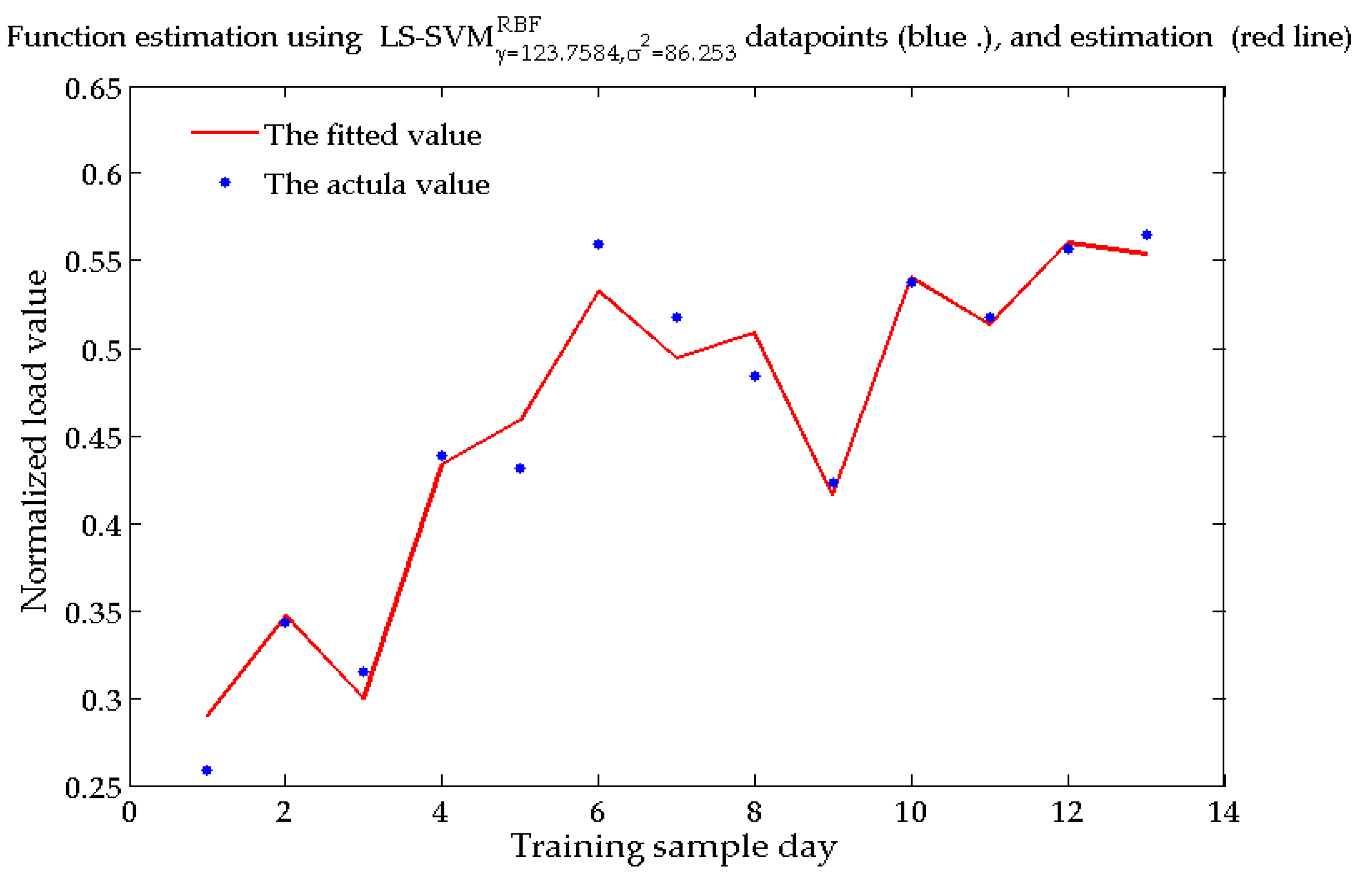
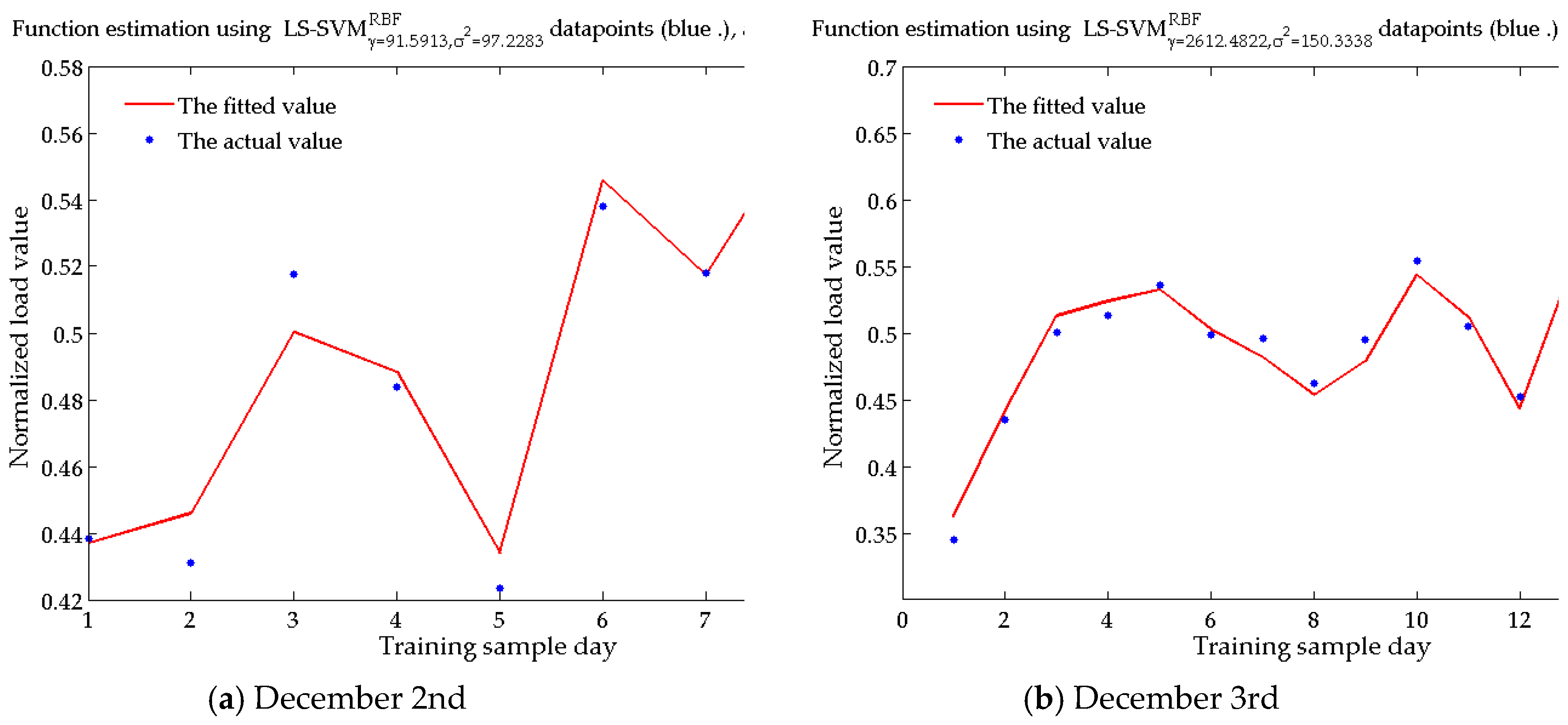
The kernel functions available for the LSSVM model include the Sigmoid kernel function, the Polynomial kernel function, and the Radial Basis Function (RBF) kernel function. The RBF kernel function has fewer preset parameters and thus can be well adapted to practical problems. Therefore, this paper adopts the RBF function as the kernel function of the LSSVM model, that is [55]:
K ( x i , x j ) = exp ( | | x i x j | | 2 σ 2 )
After selecting the appropriate kernel function K ( x i , x j ) to solve the nonlinear regression problem, Equation (11) can be solved and the following decision function can be obtained:
f ( x ) = i = 1 L λ i K ( x i , x ) + b
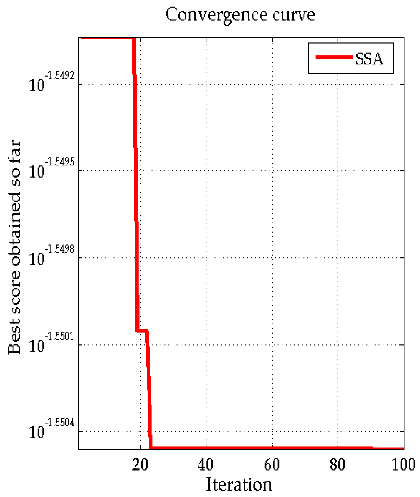
In Equation (13), there are two parameters needed to be determined, that is, the regularization parameter c and the kernel function parameter σ 2 . In order to avoid the influence of subjective factors, this paper uses the salp swarm algorithm (SSA) to automatically find the optimal values of the two parameters.
The salp is a kind of deep-sea animal that usually exhibits collective action, forming a group called the salp chain, so as to achieve better movement by quickly coordinating with the location of the food. Based on this, Australian scholar Mirjalili S proposed a new heuristic optimization method, entitled the salp swarm algorithm (SSA) [56]. In the SSA method, the initial population is divided into leaders and followers, and the leader leads the chain of the salp, followed by the followers. Assuming that there is a food source in the search space which is the salp chain target, called F , according to the behavior of the salp chain, the specific optimization steps are as follows [42,56,57]:
(1) Set the parameters. SSA mainly includes five parameters, namely, the initial number of population, the number of variables, the maximum number of iterations, the lower bound of the variable and the upper bound of the variable.
(2) Population initialization. In the SSA algorithm, the initial population of the salp group is initialized at random locations, and the position matrix is as follows:
S = [ s i j ] n × d
where s i j is the value of the j -th variable of the i -th salp, i = 1 , 2 , , n ,   j = 1 , 2 , , d , and s i j is calculated by Equation (15):
s i j = rand ( i , j ) × [ u b ( i ) l b ( i ) ] + l b ( i )
where rand ( i , j ) is a random matrix whose all elements are distributed in the [0,1] interval. u b ( i ) and l b ( i ) represent the upper and lower bounds of the i -th salp, respectively.
(3) Construct a fitness function. The fitness function is used to calculate each salp’s fitness value determined during the optimization process, and all values are stored in the matrix O S as follows:
O S = [ O S 1 O S 2 O S n ] = { f [ ( s 11 s 12 s 1 d ) ] f [ ( s 21 s 22 s 2 d ) ] f [ ( s n 1 s n 2 s n d ) ] }
In the matrix O S , the position of the salp with the best fitness value is considered as the food source F , and its position is tracked by the salp chain, so that the global optimum value can be obtained by moving the food source F .
(4) Iterative process. In order to perform a global search and avoid local optimization, all of the salps will update their positions through specific steps in the SSA method. Among them, the way the leader updates the location of the food source is:
x j 1 = { F j + c 1 [ ( u b j l b j ) c 2 + l b j ] ,   c 3 0 F j c 1 [ ( u b j l b j ) c 2 + l b j ] ,   c 3 < 0
where x j 1 represents the position of the leader (the first salp) in the j -th dimension, F j is the location of the food source, u b j and l b j represent the upper and lower bounds, respectively, and c 1 , c 2 and c 3 are all random numbers. Specifically, c 2 and c 3 are randomly generated in the interval [0,1] to determine the step size and direction of the j -th dimension moving to the next position, and c 1 is defined as follows:
c 1 = 2 e ( 4 l L ) 2
where L is the maximum number of iterations and l is the current number of iterations. The follower’s location can be updated as follows:
x j i = 1 2 ( x j i + x j i 1 )
Except for initialization, all steps are performed during the iteration until the end standard of the SSA iteration is reached.

4. Empirical Results and Interpretation

4.1. Data Sources and Pre-Processing

This paper takes the data of a city which is seriously affected by air pollution in Northern China as an example, to verify the scientific nature of the proposed short-term load forecasting model considering the impact of APPC measures. The date period is 98 days from 1 September to 7 December in 2018, of which 91 days from 1 September to 30 November in 2018 are training samples, and seven days from 1 to 7 December in 2018 are test samples.
The input variables of the short-term load forecasting model in this paper include daily air quality level, daily average air pressure, daily average temperature, daily average humidity, daily rainfall, daily average wind speed and date type, and the output variable is the daily average load. Among them, the load data is from the city power company, the meteorological data are collected through the meteorological website, and the air quality level and date type are collated by the author according to the valuing rules shown in Table 1.
Firstly, the relevant data of the above eight variables of the city from 1 September to 7 December in 2018 are collected, and the descriptive statistics of the data are shown in Table 2.
Before performing similar day selection and load forecasting, it is first necessary to normalize the data using Equation (1) to eliminate the influence of the dimension. The descriptive statistical results after standardization of variables are shown in Table 3.

4.2. Training Sample Set Construction Results

In this paper, the BWM-GRA method is used to select the similar day of the day to be predicted, so as to construct the training sample set required for load forecasting. Firstly, the BWM method is used to determine the weights of the characteristic indicators. According to the expert opinion, the daily average temperature is set as the optimal indicator, and the daily average wind speed is the worst indicator. Through an expert questionnaire survey, the preference degrees of each characteristic indicator relative to the optimal and worst indicators were obtained, as shown in Table 4.
According to Table 4 and Liu Y et al. [51], the weight of each characteristic indicator obtained by using Lingo11 is as shown in Table 5:
According to the Equations (2)–(5) and the weighting results of the characteristic indicators, the gray relational coefficient between the normalized daily characteristic indicator sequences of the day to be predicted and each similar sample day can be calculated. For example, for the 1 December, 2018, the normalized sequence is X 0 12.1 = ( 0.9524 , 0.4926 , 0.4760 , 0.6655 , 0.1103 , 0.1071 , 0.9130 ) , and for a similar sample day in the similar day sample set (e.g., 1 September 2018), the normalized sequence is X 1 = ( 0.3175 , 0.4118 , 0.9398 , 0.4835 , 0.0000 , 0.6417 , 0.9130 ) . According to the BWM-GRA method proposed in this paper, the grey relational coefficient of the two sequences is calculated to be 0.7656. Similarly, the gray relational coefficient between other similar sample day sequences and the 1 December sequence can be calculated. On this basis, according to the Delphi method [58], considering that the capacity of the training sample set should be characteristic indicator, the gray relational threshold of 1 December is set to 0.8, and a total of 13 similar days of 1 December are obtained, which constitute a set of training sample set used to forecast the load on 1 December.
Similarly, the gray relational degrees between other to-be-predicted day characteristic indicator sequences and all similar sample days’ characteristic indicator sequences can be calculated. On this basis, the threshold of the gray relational of each to-be-predicted day is set using the Delphi method, and the similar sample day whose grey relational value is greater than the given threshold is selected to constitute the training sample set of the day to be predicted. The results of similar sample day selection are shown in Table 6.

4.3. Forecasting Results

This section takes the 1 December load forecasting process as an example to demonstrate the specific application of the proposed load forecasting model.
Firstly, the 13 similar sample days corresponding to 1 December are used as training sample sets. After standardizing the data, the parameters of the LSSVM optimized by SSA are calculated by using the MATALB software, and the regularization parameter C = 123.7584 , the kernel function parameter σ 2 = 86.253 . At this time, the fitness function value of the SSA-LSSVM model is 0.0282, that is, the model fitting accuracy can reach over 97% [42]. The process of optimizing the LSSVM parameters using SSA is shown in Figure 2.
By substituting the optimized LSSVM model parameters and the relevant data of the training sample set into the model, the LSSVM model is trained, and the model fitting effect after training is shown in Figure 3.
Input the load influencing factor data of 1 December into the trained model, and the normalized load value of the day can be obtained. Then, the forecasted load value can be calculated according to Equation (1), and the forecasting accuracy of the model can be obtained by comparing the forecasted result with the actual load value, as listed in Table 7.
Similarly, using the similar day samples of forecasted days from 2 December to 7 December listed in Table 6 as the training sample set, based on the standardized data, the SSA-optimized LSSVM parameters and model fitness function value for each to-be-forecasted day can be obtained using the MATALB, which are shown in Table 8. Meanwhile, the processes of optimizing the LSSVM parameters using SSA for other to-be-forecasted days are shown in Figure 4.
By substituting the optimized LSSVM model parameters and the relevant data of the training sample set into the model, the LSSVM models for other to-be-forecasted days are trained, and the model fitting effects after training are shown in Figure 5.
The load influencing factors data of six to-be-forecasted days from 2 December to 7 December are input into the respective trained models to obtain the standardized load value for the six days, and then the predicted load values are calculated and compared with the actual load values to obtain the prediction accuracy of each model, as shown in Table 9, from which it can be seen that the forecasting accuracy of each to-be-forecasted day is less than 2%, revealing that the proposed model has good applicability in forecasting the regional daily power load considering the impacts of APPC measures.

4.4. Comparison of Results

In this paper, considering the influence of APPC measures, a short-term load forecasting model is constructed based on BWM-GRA and SSA-LSSVM techniques. In order to verify the validity of the model, this paper compares the proposed model with selected short-term load forecasting models using the same data samples. The comparison models are set as follows:
Model 1: Short-term load forecasting model proposed in this paper considering the impact of APPC measures;
Model 2: Short-term load forecasting model based on BWM-GRA and SSA-LSSVM, regardless of the impact of APPC measures;
Model 3: Considering the influence of APPC measures, use traditional GRA method to select similar day samples, and use SSA-LSSVM for short-term load forecasting;
Model 4: Considering the impact of APPC measures, a short-term load forecasting model is constructed based on BWM-GRA and PSO-LSSVM [59].
Similarly, the related data of the same city from 1 September to 30 November in 2018 are used as training samples, and those from 1 December to 7 December are used as test samples. The above model is used for prediction, and the results are shown in Table 10.
According to the actual load, the prediction error of each test sample day and the average error of each model are calculated, as shown in Figure 6, where MAPE is mean absolute percentage error, calculated by:
M A P E = 1 N i = 1 N | y i y ^ i y i |
where N is the number of the day to be forecasted, y i and y ^ i are the actual and forecasted loads of i -th to-be-forecasted day.
According to Table 10 and Figure 6, combined with the selected model scheme settings, several findings can be concluded: (1) Considering the influence of APPC measures can improve the prediction accuracy of the model. According to the comparison of models 1 and model 2, the prediction error of model 1 for each sample day to be predicted is smaller than that of model 2, and the average error of model 2 is the largest among the four models, indicating that the short-term load forecasting results of the city have significantly affected by APPC measures. Therefore, considering this impact can effectively improve the accuracy of short-term load forecasting.
(2) Using BWM-GRA to construct training samples can avoid the subjectivity of training sample construction and improve prediction accuracy. Through the comparison of Model 1 and Model 3, using the traditional GRA method to construct the training sample set does not consider the difference of the importance degree of each influencing factor, so that the training sample set has certain deviation. In model 1, the traditional GRA is improved by using BWM, revealing that the importance of each influencing factor is considered in the process of constructing the training sample set, which makes the construction result of the training sample set more realistic, helping to improve the prediction accuracy.
(3) The forecasting model based on LSSVM method has high accuracy, and using SSA to optimize parameters can reduce subjectivity and improve model prediction effect. Compared with SVM, the LSSVM-based prediction method simplifies the calculation process and has the advantage of fast and accuracy. In addition, according to the comparison between Model 1 and Model 4, although the PSO and SSA parameter optimization can both reduce the subjectivity of the model, compared with PSO, SSA can reduce the computational complexity of parameter optimization and improve the optimization efficiency by setting the leader and followers in the parameter optimization process.

5. Conclusions and Discussions

5.1. Conclusions

The implementation of APPC measures will affect the electricity consumption behaviors of power users, thus affecting the regional electricity load. However, the previous researches had less consideration on the APPC measures’ impacts on short-term load. Therefore, this paper first analyzed the background of APPC measures, and then examined the policy system of APPC measures and its impact on short-term load. Furthermore, this paper incorporated the impact of APPC measures into the load forecasting framework, and proposed a short-term load forecasting model based on BWM-GRA and SSA-LSSVM techniques. Specifically, the BWM method was adopted to improve the traditional GRA that ignores the importance difference of different characteristic indicators, so as to select similar day sample to construct the training sample set for forecasting the selected daily power load. The SSA approach was employed to optimize the parameters used in LSSVM to reduce the subjectivity of the model parameter setting process, which can reduce the computational complexity of optimization and improve the optimization efficiency.
To verify the effectiveness of the proposed model, an empirical analysis was performed based on the data of a city affected by air pollution in Northern China from 1 September to 7 December in 2018. Moreover, three selected models are employed to forecast the daily power load of the city using the same samples, and their results are compared with the proposed model’s result, which can present the performance of the proposed hybrid forecasting model. Specifically speaking: (1) The M A P E of Model 1 is less than that of Model 2, indicating that APPC measures have significant impacts on the short-term load of the city affected by air pollution, and considering this impact can effectively improve the prediction accuracy. (2) A comparison of Model 1 and Model 3 reveals that after using BWM to improve the traditional GRA method, the obtained training sample set can better reflect the characteristic similarity of the to-be-forecasted days and the training sample days, thus helping to improve the accuracy of load forecasting. (3) Using the SSA to optimize the parameters of LSSVM has the characteristics of low computational complexity, avoidance of subjectivity of model parameter setting, and thus has high prediction accuracy, as suggested by the comparison of Model 1 and Model 4.

5.2. Discussions

Although the proposed short-term load forecasting model considering the impact of APPC measures based on BWM-GRA and SSA-LSSVM techniques can be well applied to forecast the daily power load of the city affected by air pollution in Northern China, there is still room for improvement in this paper.
(1) The selection of indicators to characterize the impact of APPC measures needs further investigation. In this paper, the factor that causes APPC measures, namely the AQI is considered as a as a variable reflecting the impact of APPC measures, which is mainly based on the assumption that the value of AQI and the implementation of APPC measures have a clear and unique correspondence. However, the correspondence between AQI value and APPC measures may be ambiguous and non-unique, so how to select or construct corresponding indicators to reflect this relationship is one of the alternative directions to further improve the accuracy of short-term load forecasting under APPC measures, and is also the direction that this paper can be further improved in the future.
(2) The universality of the proposed short-term load forecasting model needs further discussions. The empirical analysis and model comparison results verify the applicability of the proposed regional short-term load forecasting model based on BWM-GRA and SSA-LSSVM techniques, and provide ideas and framework for similar forecasting problems. However, for other forecasting problems, such as renewable energy output forecasting and time-point load forecasting, the applicability of the proposed forecasting model needs to be discussed. (1) The set of influencing factors needs to be adjusted according to the forecasting object. The influencing factors of daily load forecasting in this paper include the influence of APPC measures, meteorological indicators and date types. For other forecasting problems, it is necessary to construct corresponding sets of influencing factors according to the characteristics of the objects to be forecasted. (2) There is still room for improvement in the training sample set construction method. In the proposed BWM-GRA based training sample set construction method, the method of judging the importance of factors is the BWM method, which needs to give the judgment of the importance of all indicators relative to the best and worst indicators, and thus is a weighting method under the classical set. However, for the cases where the judgment result of the indicator importance is difficult to clearly predict, the fuzzy BWM method [60] can be considered. Moreover, the threshold value of each day to be predicted in the GRA is determined based on the Delphi method, which has a certain subjectivity, so the fuzzy Delphi [61] method can be used to reduce the subjectivity of the expert experience through multiple rounds of expert feedback. (3) The choice of forecasting methods under large samples remains to be discussed. The forecasting model based on SSA optimized LSSVM has better adaptability under small samples [42,62]. When the training sample set is too large, the method may have a good fitting effect on the training samples, but the deviation of the forecasting results of the test samples may be large, indicating that the method is prone to over-fitting under large samples. Therefore, the applicability of SSA is debatable in large-sample-based forecasting issues such as renewable energy output forecasting and time-point load forecasting.
In summary, the short-term load forecasting model based on BWM-GRA and SSA-LSSVM proposed in this paper fully considers the impacts of APPC measures on regional short-term load, enriching and expanding the short-term load forecasting theory, which can provide an effective tool for short-term load forecasting. In addition, this paper uses the factor that most influences APPC measures as the policy impact variable of APPC measures, namely the air quality index; thus providing a new idea for similar research that considers policy shocks, i.e., when it is difficult to find an indicator that can characterize the policy impact, it can be considered to adopt the indicator that triggers the policy as an alternative variable to complete the analysis. Finally, there are still some improvements to be made in the construction of the influencing factors set and forecasting models in this paper, which can provide future directions for the study of forecasting issues considering policy impacts.

Author Contributions

X.L., H.Z. and B.L. conceived and designed the research method used in this paper; L.Z. and W.X. collected the data, related policy documents and reference used for the analysis; S.G. checked the language of this paper; B.L. performed the empirical analysis and wrote the paper.

Funding

This research received no external funding.

Acknowledgments

Thanks are due to the North China Electric Power University Library for providing detailed reference.

Conflicts of Interest

The authors declare no conflict of interest.

References

  1. Yang, H.; Liu, J. Research on the time-space diffusion and joint prevention and control strategy of regional compound air pollution. Mod. Bus. Trade Ind. 2018, 39, 196–197. [Google Scholar]
  2. Qin, Y.; Xie, Z.; Li, Y. Review of Research on the Impacts of Atmospheric Pollution on the Health of Residents. Environ. Sci. 2019, 40, 1512–1520. [Google Scholar]
  3. Lyu, W.; Li, Y.; Guan, D.; Zhao, H.; Zhang, Q.; Liu, Z. Driving forces of Chinese primary air pollution emissions: An index decomposition analysis. J. Clean. Prod. 2016, 133, 136–144. [Google Scholar] [CrossRef]
  4. Xie, R.; Zhao, G.; Zhu, B.Z.; Chevallier, J. Examining the factors affecting air pollution emission growth in China. Environ. Model. Assess. 2018, 23, 389–400. [Google Scholar] [CrossRef]
  5. Shi, L.; Wang, Y.; Cheng, R.; Bian, Y. Effects of industrial structure adjustment on air pollutant emission in Beijing-Tianjin-Hebei region based on the impulse response function of VAR model. Sci. Technol. Rev. 2018, 36, 24–31. [Google Scholar]
  6. China State Council. Notice of the State Council on Printing and Disclosing the Air Pollution Prevention and Control Action Plan. Available online: http://www.gov.cn/zhengce/content/2013-09/13/content_4561.htm (accessed on 10 September 2013).
  7. Zhang, H.; Wang, S.; Hao, J.; Wang, X.; Wang, S.L.; Chai, F.; Li, M. Air pollution and control action in Beijing. J. Clean. Prod. 2016, 112, 1519–1527. [Google Scholar] [CrossRef]
  8. Feng, L.; Liao, W. Legislation, plans, and policies for prevention and control of air pollution in China: Achievements, challenges, and improvements. J. Clean. Prod. 2016, 112, 1549–1558. [Google Scholar] [CrossRef]
  9. Mi, Z.F.; Pan, S.Y.; Yu, H.; Wei, Y.M. Potential impacts of industrial structure on energy consumption and CO2 emission: A case study of Beijing. J. Clean. Prod. 2015, 103, 455–462. [Google Scholar] [CrossRef]
  10. Yuan, J.; Zhang, W. Research on the quantification and de-capacity path of China’s coal-fired excess scale. Energy China 2017, 39, 14–20. [Google Scholar]
  11. Yuan, J.; Lei, Q.; Wang, Y. China’s electricity demand outlook and coal power prospect analysis under the new economic normal. Energy China 2015, 7, 21–27. [Google Scholar]
  12. Sun, Y.; Shi, M.; Shan, B.; Cao, F. Electric energy substitution potential analysis method based on particle swarm optimization support vector machine. Power Syst. Technol. 2017, 41, 1767–1771. [Google Scholar]
  13. Liu, G.; Yang, Z.; Chen, B.; Su, M.; Ulgiati, S. Prevention and control policy analysis for energy-related regional pollution management in China. Appl. Energy 2016, 166, 292–300. [Google Scholar] [CrossRef]
  14. Niu, D.; Song, Z.; Xiao, X. Electric power substitution for coal in China: Status quo and SWOT analysis. Renew. Sustain. Energy Rev. 2017, 70, 610–622. [Google Scholar] [CrossRef]
  15. Xiang, K.; Jichao, B. A Preliminary Study on Effects of Cutting Overcapacity on China’s Energy Security. J. Ind. Technol. Econ. 2018, 37, 141–147. [Google Scholar]
  16. Feng, Y.; Wang, S.; Sha, Y.; Ding, Q.; Yuan, J.; Guo, X. Coal power overcapacity in China: Province-Level estimates and policy implications. Resour. Conserv. Recycl. 2018, 137, 89–100. [Google Scholar] [CrossRef]
  17. Shanghai Securities News. North China will fight the smog this winter: Three types of enterprises like cement and steel mills in 20 cities have implemented temporary shutdowns. Ready-Mix. Concr. 2016, 11, 26. [Google Scholar]
  18. Global Plastics Network. Multi-Industries in “2+26” City Have Implemented Temporary Shutdowns Planning to Solve Air Pollution Problems. Available online: https://www.pvc123.com/news/2017-08/375070.html (accessed on 25 August 2017).
  19. Nahit, E.S.; Macfarlane, G.J.; Pritchard, C.M.; Cherry, N.M.; Silman, A.J. Short term influence of mechanical factors on regional musculoskeletal pain: A study of new workers from 12 occupational groups. Occup. Environ. Med. 2001, 58, 374–381. [Google Scholar] [CrossRef]
  20. Çevik, H.H.; Çunkaş, M. Short-term load forecasting using fuzzy logic and ANFIS. Neural Comput. Appl. 2015, 26, 1355–1367. [Google Scholar] [CrossRef]
  21. Boroojeni, K.G.; Amini, M.H.; Bahrami, S.; Iyengar, S.S.; Sarwat, A.I.; Karabasoglu, O. A novel multi-time-scale modeling for electric power demand forecasting: From short-term to medium-term horizon. Electr. Power Syst. Res. 2017, 142, 58–73. [Google Scholar] [CrossRef]
  22. Porumb, R.; Postolache, P.; Seritan, G.; Vatu, R.; Ceaki, O. Load profiles analysis for electricity market. Comput. Methods Soc. Sci. 2013, 1, 30–38. [Google Scholar]
  23. Seritan, G.; Triştiu, I.; Fierăscu, G.; Vatu, R. Assessment for Efficient Operation of Smart Grids Using Advanced Technologies. In Proceedings of the 2018 IEEE International Conference and Exposition on Electrical and Power Engineering (EPE), Iasi, Romania, 18–19 October 2018; pp. 0901–0905. [Google Scholar]
  24. Cai, S.; Wang, Y.; Zhao, B.; Wang, S.; Chang, X.; Hao, J. The impact of the “air pollution prevention and control action plan” on PM2. 5 concentrations in Jing-Jin-Ji region during 2012–2020. Sci. Total Environ. 2017, 580, 197–209. [Google Scholar] [CrossRef]
  25. Duan, L.; Niu, D.; Gu, Z. Long and medium term power load forecasting with multi-level recursive regression analysis. In Proceedings of the 2008 IEEE Second International Symposium on Intelligent Information Technology Application, Shanghai, China, 20–22 December 2008; Volume 1, pp. 514–518. [Google Scholar]
  26. Lei, S.; Sun, C.; Zhou, Q.; Zhang, X. The research of local linear model of short term electrical load on multivariate time series. In Proceedings of the 2005 IEEE Russia Power Tech, St. Petersburg, Russia, 27–30 June 2005. [Google Scholar]
  27. Cui, H.; Peng, X. Summer short-term load forecasting based on ARIMAX model. Power Syst. Prot. Control 2015, 43, 108–114. [Google Scholar]
  28. Quan, H.; Srinivasan, D.; Khosravi, A. Short-term load and wind power forecasting using neural network-based prediction intervals. IEEE Trans. Neural Netw. Learn. Syst. 2014, 25, 303–315. [Google Scholar] [CrossRef]
  29. Teo, T.T.; Logenthiran, T.; Woo, W.L. Forecasting of photovoltaic power using extreme learning machine. In Proceedings of the 2015 IEEE Innovative Smart Grid Technologies-Asia (ISGT ASIA), Bangkok, Thailand, 3–6 November 2015; pp. 1–6. [Google Scholar]
  30. Li, S.; Wang, P.; Goel, L. Short-term load forecasting by wavelet transform and evolutionary extreme learning machine. Electr. Power Syst. Res. 2015, 122, 96–103. [Google Scholar] [CrossRef]
  31. Li, S.; Goel, L.; Wang, P. An ensemble approach for short-term load forecasting by extreme learning machine. Appl. Energy 2016, 170, 22–29. [Google Scholar] [CrossRef]
  32. Ryu, S.; Noh, J.; Kim, H. Deep neural network based demand side short term load forecasting. Energies 2016, 10, 3. [Google Scholar] [CrossRef]
  33. Chen, Y.; Hong, W.C.; Shen, W.; Huang, N. Electric load forecasting based on a least squares support vector machine with fuzzy time series and global harmony search algorithm. Energies 2016, 9, 70. [Google Scholar] [CrossRef]
  34. Zhang, X.; Wang, J.; Zhang, K. Short-term electric load forecasting based on singular spectrum analysis and support vector machine optimized by Cuckoo search algorithm. Electr. Power Syst. Res. 2017, 146, 270–285. [Google Scholar] [CrossRef]
  35. Kong, W.; Dong, Z.Y.; Jia, Y.; Hill, D.J.; Xu, Y.; Zhang, Y. Short-term residential load forecasting based on LSTM recurrent neural network. IEEE Trans. Smart Grid 2017, 10, 841–851. [Google Scholar] [CrossRef]
  36. Mo, W.; Zhang, B.; Sun, H.; Hu, Z. Method to select similar days for short-term load forecasting. J. Tsinghua Univ. 2004, 44, 106–109. [Google Scholar]
  37. Zhang, B.; Zhou, B.; Shi, M.; Wei, J. Short-Term Load Forecasting Based on Grey Correlation Analysis and Random Forest Regression Model. Water Resour. Power 2017, 35, 203–207. [Google Scholar]
  38. Huang, Q.; Li, Y.; Liu, S.; Liu, P. Short-time load forecasting based on fuzzy clustering and random forest. Electr. Meas. Instrum. 2017, 54, 41–46. [Google Scholar]
  39. Niu, D.; Wei, Y. Short-term power load combinatorial forecast adaptively weighted by FHNN similar-day clustering. Autom. Electr. Power Syst. 2013, 37, 54–57. [Google Scholar]
  40. Wu, Y.; Lei, J.; Bao, L.; Li, C. Short-term load forecasting based on improved grey relational analysis and neural network optimized by bat algorithm. Autom. Electr. Power Syst. 2018, 42, 67–74. [Google Scholar]
  41. Rezaei, J. Best-worst multi-criteria decision-making method. Omega 2015, 53, 49–57. [Google Scholar] [CrossRef]
  42. Zhao, H.; Huang, G.; Yan, N. Forecasting energy-related CO2 emissions employing a novel SSA-LSSVM model: Considering structural factors in China. Energies 2018, 11, 781. [Google Scholar] [CrossRef]
  43. Zhang, B. In 2013, the smog “engaged” China. Youth Reference, A28. Available online: http://qnck.cyol.com/html/2014-01/01/nw.D110000qnck_20140101_1-28.htm (accessed on 1 January 2014).
  44. Wang, Y.; Sun, M.; Yang, X.; Yuan, X. Public awareness and willingness to pay for tackling smog pollution in China: A case study. J. Clean. Prod. 2016, 112, 1627–1634. [Google Scholar] [CrossRef]
  45. Ma, W. Ozone Pollution Hits Beijing-Tianjin-Hebei and Has Replaced PM2.5 as a Primary Pollutant. Available online: http://www.sohu.com/a/142000958_116062 (accessed on 20 May 2017).
  46. Phoenix News. China’s Emissions of Almost All Pollutants Ranked First in the World. Available online: http://news.ifeng.com/a/20161206/50368423_0.shtml (accessed on 6 December 2016).
  47. Jin, Y.; Andersson, H.; Zhang, S. Air pollution control policies in China: A retrospective and prospects. Int. J. Environ. Res. Public Health 2016, 13, 1219. [Google Scholar] [CrossRef] [PubMed]
  48. Zhang, J.; Jiang, H.; Liu, G.; Zeng, W. A study on the contribution of industrial restructuring to reduction of carbon emissions in China during the five Five-Year Plan periods. J. Clean. Prod. 2018, 176, 629–635. [Google Scholar] [CrossRef]
  49. Ministry of Environmental Protection. Environmental Air Quality Index Technical Regulations (Trial). Available online: https://wenku.baidu.com/view/5bbdd248e518964bcf847c61.html (accessed on 29 February 2016).
  50. Rezaei, J. Best-worst multi-criteria decision-making method: Some properties and a linear model. Omega 2016, 64, 126–130. [Google Scholar] [CrossRef]
  51. Liu, Y.; Li, F.Y.; Wang, Y.; Yu, X.; Yuan, J.; Wang, Y.W. Assessing the Environmental Impact Caused by Power Grid Projects in High Altitude Areas Based on BWM and Vague Sets Techniques. Sustainability 2018, 10, 1768. [Google Scholar] [CrossRef]
  52. Wang, H.; Hu, D. Comparison of SVM and LS-SVM for regression. In Proceedings of the 2005 IEEE International Conference on Neural Networks and Brain, Beijing, China, 13–15 October 2005; Volume 1, pp. 279–283. [Google Scholar]
  53. Adankon, M.M.; Cheriet, M. Model selection for the LS-SVM. Application to handwriting recognition. Pattern Recognit. 2009, 42, 3264–3270. [Google Scholar] [CrossRef] [Green Version]
  54. Carmeli, C.; De Vito, E.; Toigo, A. Vector valued reproducing kernel Hilbert spaces of integrable functions and Mercer theorem. Anal. Appl. 2006, 4, 377–408. [Google Scholar] [CrossRef]
  55. Hamers, B.; Suykens, J.A.K.; De Moor, B. Compactly supported RBF kernels for sparsifying the gram matrix in LS-SVM regression models. In Proceedings of the International Conference on Artificial Neural Networks, Madrid, Spain, 28–30 August 2002; Springer: Berlin/Heidelberg, Germany, 2002; pp. 720–726. [Google Scholar]
  56. Mirjalili, S.; Gandomi, A.H.; Mirjalili, S.Z.; Saremi, S.; Faris, H.; Mirjalili, S.M. Salp Swarm Algorithm: A bio-inspired optimizer for engineering design problems. Adv. Eng. Softw. 2017, 114, 163–191. [Google Scholar] [CrossRef]
  57. Sayed, G.I.; Khoriba, G.; Haggag, M.H. A novel chaotic salp swarm algorithm for global optimization and feature selection. Appl. Intell. 2018, 48, 3462–3481. [Google Scholar] [CrossRef]
  58. Okoli, C.; Pawlowski, S.D. The Delphi method as a research tool: An example, design considerations and applications. Inf. Manag. 2004, 42, 15–29. [Google Scholar] [CrossRef]
  59. Gorjaei, R.G.; Songolzadeh, R.; Torkaman, M.; Safari, M.; Zargar, G. A novel PSO-LSSVM model for predicting liquid rate of two phase flow through wellhead chokes. J. Nat. Gas Sci. Eng. 2015, 24, 228–237. [Google Scholar] [CrossRef]
  60. Guo, S.; Zhao, H. Fuzzy best-worst multi-criteria decision-making method and its applications. Knowl.-Based Syst. 2017, 121, 23–31. [Google Scholar] [CrossRef]
  61. Zhao, H.; Li, N. Optimal siting of charging stations for electric vehicles based on fuzzy Delphi and hybrid multi-criteria decision making approaches from an extended sustainability perspective. Energies 2016, 9, 270. [Google Scholar] [CrossRef]
  62. Abbassi, R.; Abbassi, A.; Heidari, A.A.; Mirjalili, S. An efficient salp swarm-inspired algorithm for parameters identification of photovoltaic cell models. Energy Convers. Manag. 2019, 179, 362–372. [Google Scholar] [CrossRef]
Figure 1. The policy system of APPC measures.
Sustainability 11 02983 g001
Figure 2. The process of optimizing the LSSVM parameters using SSA for 1 December.
Sustainability 11 02983 g002
Figure 3. SSA-LSSVM model fitting effect for 1 December.
Sustainability 11 02983 g003
Figure 4. Processes of optimizing LSSVM parameters using SSA for other to-be-forecasted days.
Sustainability 11 02983 g004
Figure 5. SSA-LSSVM model fitting effects for other to-be-forecasted days.
Sustainability 11 02983 g005aSustainability 11 02983 g005b
Figure 6. Forecasting error of each model.
Sustainability 11 02983 g006
Table 1. Variables and valuing rules.
Variable NameUnitValuing Rule
Daily average loadMWDaily data, actual values
Daily air quality level/0 for 0 AQI < 100 , 1 for 100 AQI < 150 , 2 for 150 AQI < 200 , and 3 for AQI 200
Daily average air pressurekPaDaily data, actual values
Daily average temperature°CDaily data, actual values
Daily average humidityg/m3Daily data, actual values
Daily rainfallmmDaily data, actual values
Daily average wind speedm/sDaily data, actual values
Date type/1 for normal working days, and 2 for legal holidays
Table 2. Descriptive statistics of sample data.
NMax.Min.MeanS.D.
Daily average load983859.62582315.0776 2922.2208 270.7487
Daily air quality level983.00000.0000 0.4286 0.8582
Daily average air pressure981018.1583983.7583 1000.1516 5.9333
Daily average temperature9826.6583−4.8958 14.9207 6.6357
Daily average humidity9897.416724.2917 58.1798 17.4024
Daily rainfall983.40830.8792 1.9854 0.5465
Daily average wind speed9819.00000.0000 0.9560 3.1773
Date type9821.0000 1.3297 0.4727
Table 3. Descriptive statistics of standardized sample data.
Variable NameNMax.Min.MeanS.D.
Z-daily average load980.89590.06250.39010.1461
Z-daily air quality rating980.95240.00000.13610.2724
Z–daily average air pressure980.62150.36570.48760.0441
Z–daily average temperature980.95980.00740.60550.2003
Z- daily average humidity980.93850.01530.44320.2197
Z-daily rainfall980.93790.01600.41920.1992
Z- daily average wind speed980.95240.00000.04790.1593
Z-date type980.91300.04350.33010.4110
Table 4. Preference degrees of each indicator relative to the best and worst indicators.
Index S 1 S 2 S 3 S 4 S 5 S 6 S 7
A B 2415483
A W 6475316
Table 5. Weights and rankings of each characteristic indicator.
Index S 1 S 2 S 3 S 4 S 5 S 6 S 7
w j 0.19370.12880.25750.08590.11190.02860.1936
Ranking2416573
Table 6. Results of similar sample day selection.
Forecasted DayGrey Relational ThresholdSimilar Sample Days *Sample Set Capacity
1 December0.81014, 1020, 1021, 1110, 1111, 1117, 1118, 1124, 1125, 1127–113013
2 December0.81110, 1111, 1118, 1124, 1125, 1127–11309
3 December0.81016, 1105–1108, 1112-1116, 1123, 1126–113016
4 December0.851016, 1025, 1105–1108, 1112, 1113 1114, 1116, 112311
5 December0.850918, 0928, 1009–1011, 1017–1019, 1026, 1029–1031, 1105–1109, 1112, 1115, 1116, 112221
6 December0.81008–1012, 1015, 1017–1019, 1026, 1029–1031, 1105–1109, 1115, 1116, 112221
7 December0.81009–1012, 1017–1019, 1026, 1029–1031, 1105–1109, 115, 1116, 112219
Note: * The similar sample days in Table 6 are expressed in the form of "month-day", for instance, 0918 is September 18, 1014 is October 14, 1105 is November 5, and 1127–1130 is from 27 November to 30 November.
Table 7. Short-term load forecast results of 1 December based on SSA-LSSVM.
Forecasted DayStandardized ValuePredictive Load (MW)Actual Load (MW)Prediction Error (%)
1 December0.47723083.65903129.3984−1.4616
Table 8. Training results of the SSA-LSSVM model.
Forecasted DayRegularization ParameterKernel Function ParameterFitness Function Value
2 December91.591397.22830.0474
3 December2612.4822150.33380.0372
4 December547.552824.14240.0382
5 December1245.0968991.93930.0750
6 December4948.3211503.33840.0888
7 December1209856.38850.0193
Table 9. Short-term load forecasting results based on SSA-LSSVM.
Forecasted DayStandardized ValuePredictive Load (MW)Actual Load (MW)Prediction Error (%)
2 December0.39532931.92442978.5803−1.5664
3 December0.53363188.29003147.44151.2978
4 December0.60663323.58323279.07151.3574
5 December0.73533562.08943599.4933−1.0391
6 December0.79323669.42333717.9822−1.3061
7 December0.86663805.32643859.6258−1.4069
Table 10. Forecasting results of each model.
Forecasted DayModel 1Model 2Model 3Model 4Actual
1 December3083.6593235.043215.653183.533129.3984
2 December2931.92443162.813122.43043.852978.5803
3 December3188.293334.163293.263249.273147.4415
4 December3323.58323448.23349.063220.623279.0715
5 December3562.08943699.983643.763507.193599.4933
6 December3669.42333842.453870.983815.773717.9822
7 December3805.32643947.513723.23778.313859.6258

