Article

Multiobjective Genetic Algorithm-Based Optimization of PID Controller Parameters for Fuel Cell Voltage and Fuel Utilization

1
Key Lab of Energy Thermal Conversion and Control of Ministry of Education, School of Energy and Environment, Southeast University, Nanjing 210096, China
2
School of Information Engineering, Ningxia University, Yinchuan 750021, China
3
College of Nuclear Science and Technology, Beijing Normal University, Beijing 100875, China
4
Department of Electrical & Computer Engineering, Baylor University, Waco, TX 76798, USA
*
Authors to whom correspondence should be addressed.
Sustainability 2019, 11(12), 3290; https://0-doi-org.brum.beds.ac.uk/10.3390/su11123290
Submission received: 20 April 2019 / Revised: 6 June 2019 / Accepted: 6 June 2019 / Published: 14 June 2019

Abstract

:
Nowadays, given the great deal of fossil fuel consumption and associated environmental pollution, solid oxide fuel cells (SOFCs) have shown their great merits in terms of high energy conversion efficiency and low emissions as a stationary power source. To ensure power quality and efficiency, both the output voltage and fuel utilization of an SOFC should be tightly controlled. However, these two control objectives usually conflict with each other, making the controller design of an SOFC quite challenging and sophisticated. To this end, a multi-objective genetic algorithm (MOGA) was employed to tune the proportional–integral–derivative (PID) controller parameters through the following steps: (1) Identifying the SOFC system through a least squares method; (2) designing the control based on a relative gain array (RGA) analysis; and (3) applying the MOGA to a simulation to search for a set of optimal solutions. By comparing the control performance of the Pareto solutions, satisfactory control parameters were determined. The simulation results demonstrated that the proposed method could reduce the impact of disturbances and regulate output voltage and fuel utilization simultaneously (with strong robustness).

1. Introduction

Nowadays, with a great deal of fossil fuel consumption, many environmental issues have been raised. With the merits of low pollution and high efficiency [1], hydrogen energy-based fuel cells are considered to be ideal alternative energy sources, and they are widely used to supply power to stand-alone power systems and vehicles [2,3,4]. Among all fuel cells, solid oxide fuel cells (SOFCs) attract much attention for their multifuel capabilities and potential for cogeneration [5], as well as their ease of coordination with refinery hydrogen networks [6]. Numerous studies about SOFCs have been done. Rao et al. [7] analyzed the thermodynamic characteristics and techno-economic performance of a system consisting of an SOFC–gas turbine system, Xia et al. [8] studied low-temperature operations of SOFCs, and Wang et al. [9] modified the anode material to solve the problem of coke formation. Besides these, studies on efficient control strategies to ensure the safety, stability, and efficiency of SOFCs are also very important. In order to maintain the efficiency of an SOFC, fuel utilization in an SOFC must be kept between 70% and 90% [10]. In addition, to ensure the power quality of an SOFC, the output voltage must be controlled tightly. However, due to the nonlinearity and couplings of multiple variables and frequent load disturbances, the control of an SOFC is extremely hard, and the controller must be appropriately designed. As a result, designing an efficient control scheme is of great significance in the research on SOFCs.
To solve the problem of maintaining the output voltage and fuel utilization of SOFCs, many advanced control strategies have been proposed, such as model predictive control (MPC) [11,12,13], fuzzy proportional–integral–derivative (PID) control [14], fuzzy logic control [15], and neural network control [16]. All of these control strategies have been shown to obtain excellent control performance in numerous simulation studies: However, due to their computational complexity, these control strategies are difficult to implement in practical applications.
With the merits of a simple structure and high reliability, PID controllers are widely used in the process industry: However, to ensure control performance, the control parameters of PID controllers must be tuned well. To this end, numerous artificial intelligence (AI)-based optimization methods have been applied to tune PID controllers. For example, Qin, Sun, and Hua [17] used a fruit fly optimization algorithm (FOA) to optimize the PID controllers of a refrigeration system, Zamani et al. [18] applied a particle swarm optimization (PSO) algorithm to optimize the PID controller of an automatic voltage regulator (AVR), and Elbayomy et al. [19] optimized the PID controller of an electrohydraulic servo actuator system (EHSAS) to control the movable surface of a space vehicle. However, these references all used a single-objective optimization method, where the authors judged a controller’s performance through one objective function that weighted the sum of different performance indices, such as the integral absolute error (IAE), overshoot, and settling time. Although in the end this method achieved good results, it ignored the problem that the control objectives were usually conflicting and that the weight factors were decided subjectively by the author. Instead of using only one objective function, a Pareto-based multiobjective optimization algorithm involves two or more objective functions and is thus able to deal with the conflicting objectives of a control system without designating weight factors: Many researchers choose this method to solve optimization problems [20,21,22,23].
This paper aims to (1) identify a dynamic SOFC model as a linearized model, (2) apply two PID controllers to maintain the output voltage and fuel utilization of an SOFC under load disturbance, and (3) enhance the control system performance by optimizing the controller with multiobjective optimization. The remaining part of this paper is organized as follows: In Section 2, a dynamic SOFC model is introduced, while in Section 3, a linearized model is identified and a controller for the model is designed. Section 4 optimizes the controller parameters with genetic algorithm (GA)-based multiobjective optimization, and Section 5 applies the optimal controllers to the nonlinear system and analyzes the optimization results. Conclusions are drawn in Section 6.

2. Problem Description

2.1. Dynamic Model for an SOFC

The model presented in this paper was based on three submodels: An electrochemical model, a mass balance model, and an energy balance model. To simplify the model, six assumptions were made as follows:
  • Both hydrogen and air are preheated to a specific temperature before entering the anode and cathode;
  • Both hydrogen and air are in full contact with the anode and cathode, and the stoichiometric quantity of oxygen at the cathode is sufficiently large;
  • A large stoichiometric quantity of oxygen exists at the cathode;
  • The oxygen concentration in the air is 21%;
  • The whole stack can be presented as a combination of individual stacks;
  • Ideal gas laws are employed for both the fuel flow and air flow.
A structural diagram of this model is shown in Figure 1, where the fuel flow, air flow, oxygen ion flow, and electron flow are represented by red, blue, yellow, and green arrows, respectively.

2.1.1. Electrochemical Model

As we can tell from Figure 1, the SOFC consists of an anode and a cathode, and they are connected by a solid ceramic electrolyte. Through the electrolyte, oxygen ions are transported from the cathode to the anode, and electrons are transported from the anode to the cathode through the external electric circuit. The reaction on the anode and the cathode and the total reaction are shown as follows:
2 H 2 + 2 O 2 2 H 2 O + 4 e ,
O 2 + 4 e 2 O 2 ,
2 H 2 + O 2 H 2 O .
Based on Nernst’s equation [14], the open circuit voltage of the fuel cell stack Ecell can be formulized as
E c e l l = E 0 , c e l l + R T c e l l 2 F ln [ p H 2 p O 2 0.5 p H 2 O ] .
Here, E0,cell can be calculated as
E 0 , c e l l = E 0 , c e l l 0 k E ( T 298 ) ,
where E 0 , c e l l 0 is the reference voltage at 298 K and 1 atm of pressure.
The partial pressures in Equation (4), pH2, pO2, and pH2O, are the average of the inlet and outlet partial pressures of the respective components, calculated as follows:
p H 2 = p H 2 i n + p H 2 o u t 2 ,
p O 2 = p O 2 i n + p O 2 o u t 2 ,
p H 2 O = p H 2 O i n + p H 2 O o u t 2 .
Due to ohmic loss, activation loss, and concentration loss, the output voltage of the fuel cell stack Vcell is lower than Ecell, which is calculated as
V c e l l = E c e l l V o h m V a c t V c o n .
The expression of the three voltage drops are given below:
V o h m = I A c e l l R o h m ,
V a c t = R T F ( sinh 1 ( I 2 i 0 , a n ) + sinh 1 ( I 2 i 0 , c a ) ) ,
V c o n = R T 2 F ( ln ( p H 2 O , r p H 2 p H 2 O p H 2 , r ) + 1 2 ln ( p O 2 p O 2 , r ) ) ,
where Rohm is the internal resistance of the fuel cell, and it is calculated as follows [24]:
R o h m = ( a e l e exp ( b e l e T ) A c e l l ) δ e l e + ( a i t c exp ( b i t c T ) A c e l l ) δ i t c .
According to assumption 5, the output voltage of the fuel cell can be calculated with Vcell by
V o u t = N V c e l l ,
where N is the number of fuel cells in a series.

2.1.2. Mass Balance Model

According to assumption 5, the dynamic effective partial pressure of H2, O2, and H2O can be presented as follows [25]:
V a n R T d p H 2 c h d t = M H 2 i n M H 2 o u t I 2 F ,
V a n R T d p H 2 O c h d t = M H 2 O i n M H 2 O o u t + I 2 F ,
V c a R T d p O 2 c h d t = M O 2 i n M O 2 o u t I 2 F ,
while based on assumption 2, the inlet and outlet mass flow rate of H2, O2, and H2O can be described as
{ M H 2 i n = M a n x H 2 i n = M a n p H 2 i n p a n c h M H 2 o u t = M a n x H 2 o u t = M a n p H 2 o u t p a n c h ,
{ M H 2 O i n = M a n x H 2 O i n = M a n p H 2 O i n p a n c h M H 2 O o u t = M a n x H 2 O o u t = M a n p H 2 O o u t p a n c h ,
{ M O 2 i n = M c a x O 2 i n = M a n p O 2 i n p c a c h M O 2 o u t = M c a x O 2 o u t = M a n p O 2 o u t p c a c h .

2.1.3. Energy Balance Model

As Figure 1 shows, hydrogen flows through the anode surface and changes into water, while air is provided by a central air supply tube (AST) and is forced to flow through the cathode. Due to the simplification of the model, the means of heat transfer inside the cell are radiation, convection, and mass flow [26].
Therefore, the energy balance equations for different parts of the cell are shown as follows:
  • Cell tube:
    q c e l l , i n = q g e n = q c h e m q e l e ,
    q c e l l , o u t = q r a d + q c o n v , a n n + q f l o w , a i r , a n n + q c o n v , f u e l + q f l o w , f u e l ,
    q c e l l , n e t = q c e l l , i n q c e l l , o u t = m c e l l C c e l l d T c e l l d t ,
    q r a d = ε A S T σ A A S T , o u t e r ( T c e l l 4 T A S T 4 ) ,
    q c o n v , a n n = h c e l l A c e l l , i n n e r ( T c e l l T a i r , a n n ) ,
    q f l o w , a i r , a n n = M a i r x a i r C a i r ( T a i r , a n n , i n T a i r , a n n , o u t ) ,
    q c o n v , f u e l = h c e l l A c e l l , o u t e r ( T c e l l T f u e l ) ,
    q f l o w , f u e l = ( M H 2 , i n + M H 2 , o u t ) x H 2 C H 2 ( T f u e l , o u t T f u e l , i n ) + ( M H 2 O , i n + M H 2 O , o u t ) x H 2 O C H 2 O ( T f u e l , o u t T f u e l , i n ) ;
  • Fuel:
    q f u e l , n e t = m f u e l C f u e l d T f u e l d t ;
  • Air between the cell tube and the AST:
    q a i r , a n n , n e t = m a i r , a n n C a i r d T a i r , a n n d t ;
  • AST:
    q A S T , n e t = m A S T C A S T d T A S T d t ,
    q A S T , c o n v , o u t e r = h A S T , o u t e r A A S T , o u t e r ( T a i r , c e l l T A S T ) ,
    q A S T , c o n v , i n n e r = h A S T , i n n e r A A S T , i n n e r ( T A S T T a i r , A S T ) ,
    q f l o w , a i r , A S T = m a i r C a i r ( T a i r , A S T , i n T a i r , A S T , o u t ) ;
  • Air in the AST:
    q a i r , A S T , n e t = m a i r , A S T C a i r d T a i r , A S T d t .
Based on the formulation of (21)–(35), the energy balance model for the SOFC was developed.

2.2. Control Problems

The main propose of the controller design was to ensure that the output voltage Vout and the fuel utilization FU follow their reference values and maintain their stability as strongly as possible. The main problems in the controller design are listed as follows:
  • High coupling: The SOFC is a coupled system, which makes its controller design challenging and complicated;
  • Frequent disturbance: Due to the frequent change of the load, a continual disturbance exists in the system, which requires the controller to have strong robustness and accurate control performance;
  • Conflicting objectives: The accuracy of the control performance of Vout and FU are the two conflicting objectives. However, to improve the power quality of the SOFC, both objectives need to be optimized at the same time.

3. Controller Design

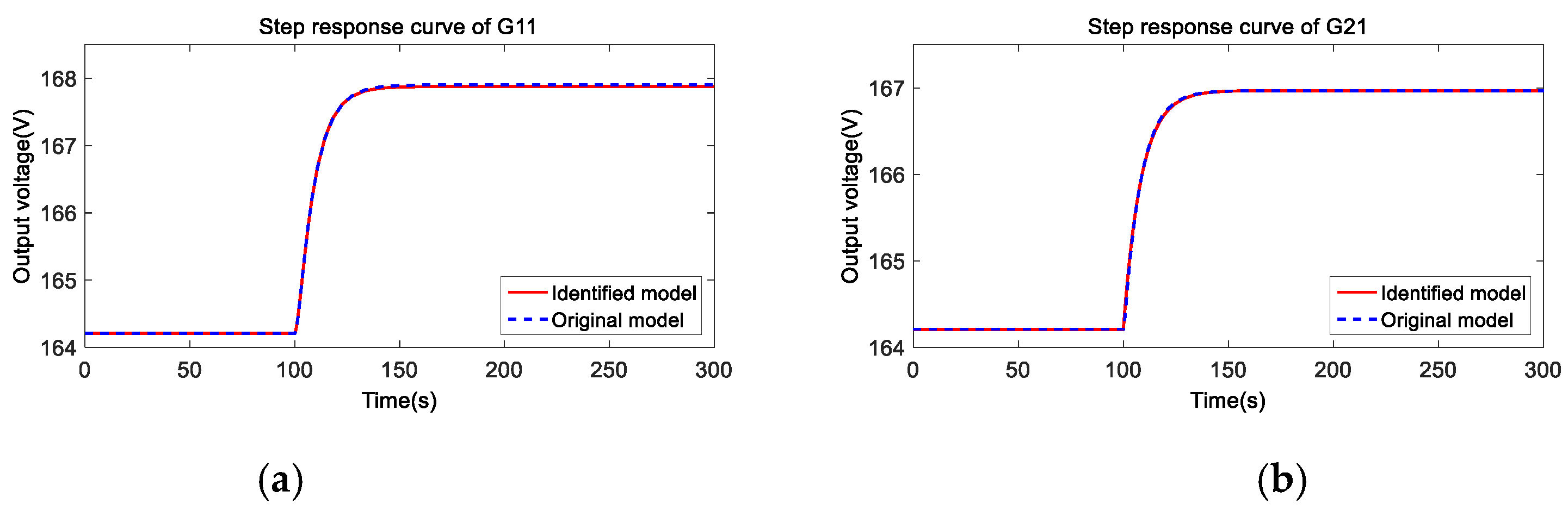
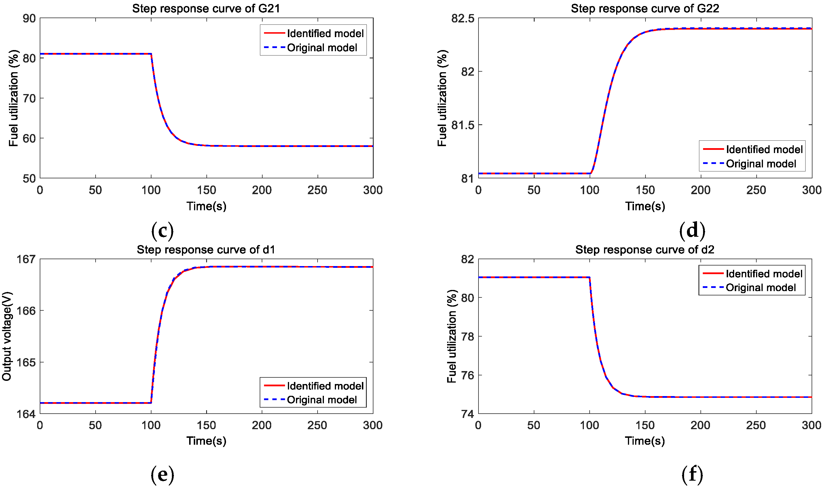
3.1. Model Identification

Since the SOFC model is a multi-input–multi-output (MIMO) system, the load resistance R was chosen as the disturbance of the system, the fuel flow mH2 and the cathode pressure Pc were chosen as the control variables, and the output voltage Vout and fuel utilization FU were chosen as the controlled variables. Thus, the linearized model can be identified as a 3 × 2 MIMO system:
[ y 1 y 2 ] = [ G 11 G 12 G 21 G 22 ] [ u 1 u 2 ] + [ G d 1 G d 2 ] d ,
where y1 is the output voltage Vout, y2 is the fuel utilization FU, u1 is the fuel flow mH2, u2 is the cathode pressure Pc, d is the load resistance R, G11 represents the transfer function from mH2 to Vout, G12 represents the transfer function from mH2 to FU, G21 represents the transfer function from Pc to Vout, G22 represents the transfer function from Pc to FU, Gd1 represents the transfer function from R to Vout, and Gd2 represents the transfer function from R to FU.
To identify these transfer functions, a step response of this system was analyzed. First, a step signal was set on mH2, while Pc and R were kept as constants, and the step responses of Vout and FU were recorded. Second, a step signal was set on Pc, while mH2 and R were kept as constants, and then the step responses of Vout and FU were recorded. Third, a step signal was set on R, while Pc and mH2 were kept as constants, and the step responses of Vout and FU were recorded. Finally, based on the step response results, the transfer functions can be readily identified as follows:
G 11 = 528.942 s + 2594.573 s 2 + 0.627 s + 0.064 G 21 = 0.108 s + 1.024 × 10 4 s 2 + 0.118 s + 1.119 × 10 4 G 12 = 271.283 s 0.286 s 2 + 0.107 s + 1.116 × 10 4 G 22 = 8.998 × 10 6 s 5.227 × 10 5 s 2 + 0.209 s + 0.012 G d 1 = 0.591 s + 5.122 × 10 4 s 2 + 0.113 s + 9.991 × 10 5 G d 2 = 0.015 s 1.306 × 10 5 s 2 + 0.121 s + 1.050 × 10 4
The step response curves are drawn in Figure 2. As we can tell from the results, the step response curves of the identified model are the same as those of the original model, and thus the identified model is able to be used for control design.

3.2. Relative Gain Array (RGA) Paring

To analyze the relationship between the input and output variables of a system, we applied the relative gain array (RGA) defined by Skogestad and Postlethwaite in [27]. First, by setting the time s to 0, we got the steady-state matrix of G11, G12, G21, and G22:
A = [ G 11 | s 0 G 12 | s 0 G 21 | s 0 G 22 | s 0 ] = [ 4.0763 × 10 4 0.9148 2.5607 × 10 3 0.0045 ] .
Then, the RGA matrix was calculated:
R G A = A ( A 1 ) T = [ λ 11 λ 12 λ 21 λ 22 ] = [ 0.0729 0.9271 0.9271 0.0729 ] .
The results show that the output voltage Vout is affected more by the cathode pressure Pc, while the fuel utilization FU is affected more by the fuel flow mH2. Thus, Vout can be controlled by Pc easily, and FU can be controlled by mH2 easily.

3.3. Controller Design

In this paper, two PID controllers were applied to control mH2 and Pc independently. The formula for a PID controller is shown as
G ( s ) = k p + k i 1 s + k d T d 1 + T d 1 s ,
where kp, ki, and kd are the proportional gain, integral gain, and derivative gain, respectively. In previous research, the main work has been to search for the optimal values of kp, ki, and kd [17,19,28]. However, the filter coefficient N is also of great importance, and an appropriate filter coefficient can reduce the output oscillation and improve the control performance. As a result, the filter coefficient was also studied for this paper, and there were eight parameters that needed to be decided on, which were the parameters of PID1 (kp1, ki1, kd1, N1) and the parameters of PID2 (kp2, ki2, kd2, N2).
The structure of the control system is shown in Figure 3, and the parameters of the controllers were initialized by the pidTuner Toolbox in Matlab as
{ k p 1 = 1.646 × 10 4 k i 1 = 1.360 × 10 4 k d 1 = 5.848 × 10 6 T d 1 = 16.970 , { k p 2 = 1.572 k i 2 = 0.326 k d 2 = 0.067 T d 2 = 1.012 .

4. Solution Method

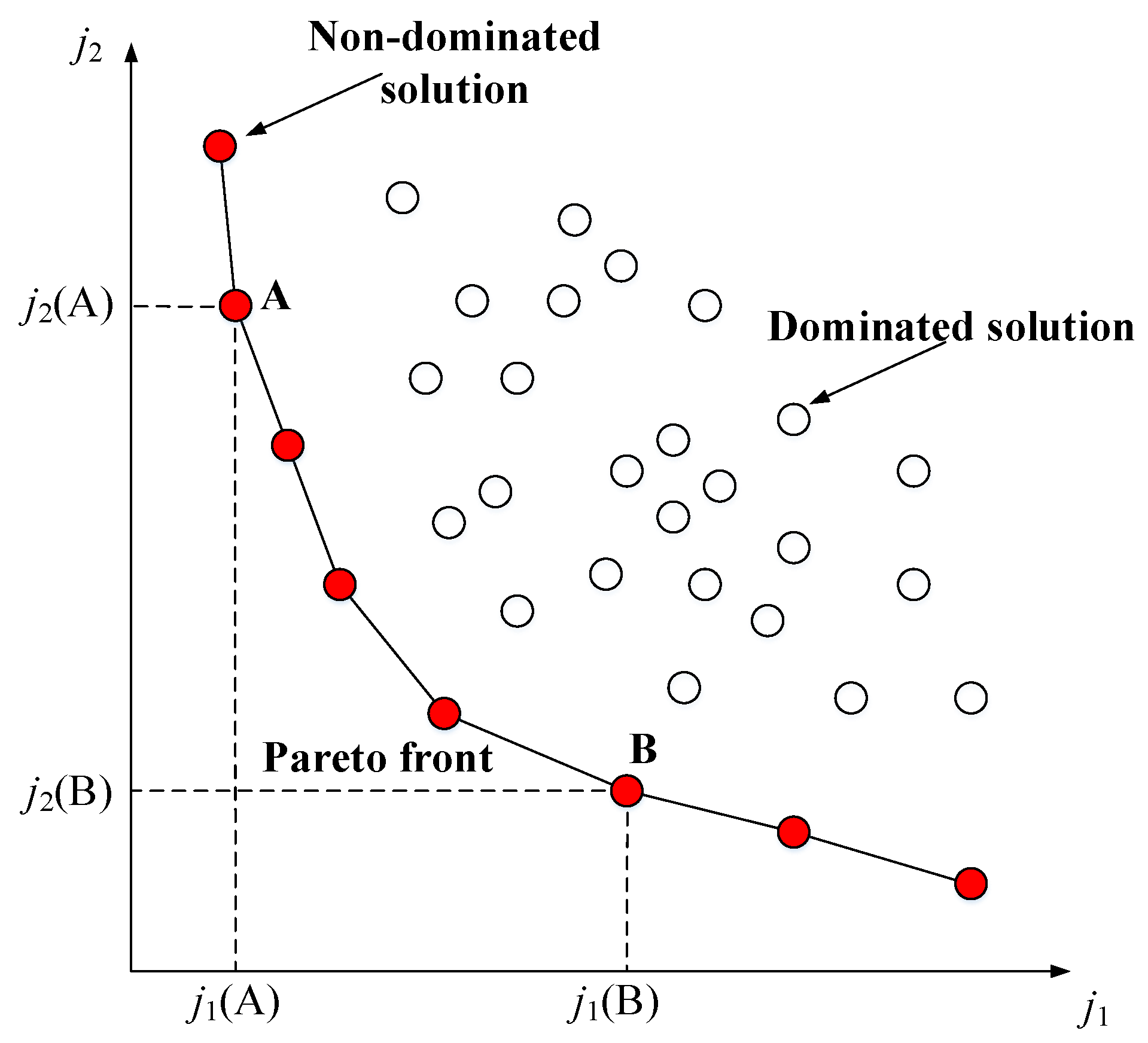
4.1. Introduction of Multiobjective Optimization based on a Genetic Algorithm

Multiobjective optimization usually involves two or more objective functions, and it is widely used in the field, where objectives are conflicting and need to be optimized at the same time. As is shown in Figure 4, the optimization result is a set of Pareto optimal solutions, where none of the objectives can be promoted without deteriorating other objectives. A multiobjective optimization problem (MOP) can be described as
min J ( x ) = [ j 1 ( x ) , j 1 ( x ) , , j n ( x ) ] x X ,
where J is the vector of objective functions, n is the number of objective functions, x represents the decision vector, and X is the constraint of the decision vector x. The objective functions are designed by the decision-maker to judge the quality of the solution, and in the field of industrial control, objective functions usually consist of an IAE, overshoot, and settling time.
To solve optimization problems, many methods have been developed, and the GA proposed by Holland in 1975 [29] is one of the most popular ones. Meanwhile, in 1994, Srinivas and Deb [30] developed a new algorithm based on a GA called a nondominated sorting genetic algorithm (NSGA), and then in 2000, an improved version of the NSGA (called the NSGA-II) was developed by Deb et al. [31]. With the merits of low computational complexities and the ability of parallel computation, it is widely used for MOPs [21,32]. Afterwards, in order to improve the distribution density of the Pareto front and avoid the problem of premature ripening, an improved NSGA-II was developed by introducing the parameter Pareto faction x, which represents the ratio of the optimal solutions to the total population (Equation (43)):
x = N Pareto N ,
where N represents the population size, and NPareto represents the number of Pareto optimal solutions. A flow chart of this algorithm is shown in Figure 5.
In this section, the proposed improved NSGA-II is applied to find the optimal sets of control parameters for the SOFC.

4.2. Optimization of the Control Parameters of the SOFC

As was mentioned in Section 3, there were eight parameters in the two PID controllers that needed to be optimized: kp1, ki1, kd1, N1, kp2, ki2, kd2, and N2. Thus, the decision vector could be described as x = (kp1, ki1, kd1, N1, kp2, ki2, kd2, N2). The integral absolute error (IAE) of the output voltage and fuel utilization were employed as two objective functions, and the MOP could be formulated as
min F = [ I A E 1 ( x ) I A E 2 ( x ) ] ,
where
I A E 1 = 0 T ( | V out , ref V out | ) d t ,
I A E 2 = 0 T ( | F U ref F U | ) d t ,
and the constraint for each parameter is shown as
{ k p 1 ( 10 2 , 10 7 ) k i 1 ( 10 2 , 10 7 ) k d 1 ( 10 8 , 10 4 ) T d 1 ( 10 3 , 100 ) , { k p 2 ( 10 3 , 10 ) k i 2 ( 10 3 , 10 ) k d 2 ( 1 , 10 4 ) T d 2 ( 10 3 , 100 ) .
The population size N was set as 50, the maximum generation Max was set as 50, the Pareto fraction x was set as 0.35, the mutation function was a constraint-dependent type, and the crossover probability was 0.8. The stopping criteria were designed as follows:
  • The number of generations is higher than the maximum number of iterations;
  • The average relative change in the spread of the Pareto solutions over 100 generations is less than 10−4, and the spread is smaller than the average spread over the last 100 generations.
For each generation, four load disturbances occurred in each simulation process, and two objective functions, IAE1 and IAE2, of 50 individuals were calculated based on the simulation results.
The distribution of the final population in the objective function space is shown in Figure 6, which clearly illustrates the conflicting relationship between IAE1 and IAE2. Any decrease in IAE2 led to an increase in IAE1. In other words, any improvement in the control performance of fuel utilization led to a deterioration in the control performance of the output voltage. Five typical points were chosen from the Pareto front to get the optimal parameters of the controllers, and the value of each parameter and the objective function are displayed in Table 1. In Table 1, point A possessed the lowest IAE1 and the highest IAE2, while point E possessed the highest IAE1 and the lowest IAE2. As we can tell, there were trade-offs between the two objectives, and to decide the final optimal solution, a decision-making process should be executed based on the decision-maker’s insight.
Figure 7 denotes the variation of the objective functions with the generation. As we can tell from the result, IAE1 decreased from 22.75 to 1.20 and converged at about 1.197 after 30 generations, while IAE2 decreased from 0.8 to 0.011 and converged at about 0.0108 after 25 generations. Both IAE1 and IAE2 were greatly minimized after about 30 generations, and thus the optimization was successful.

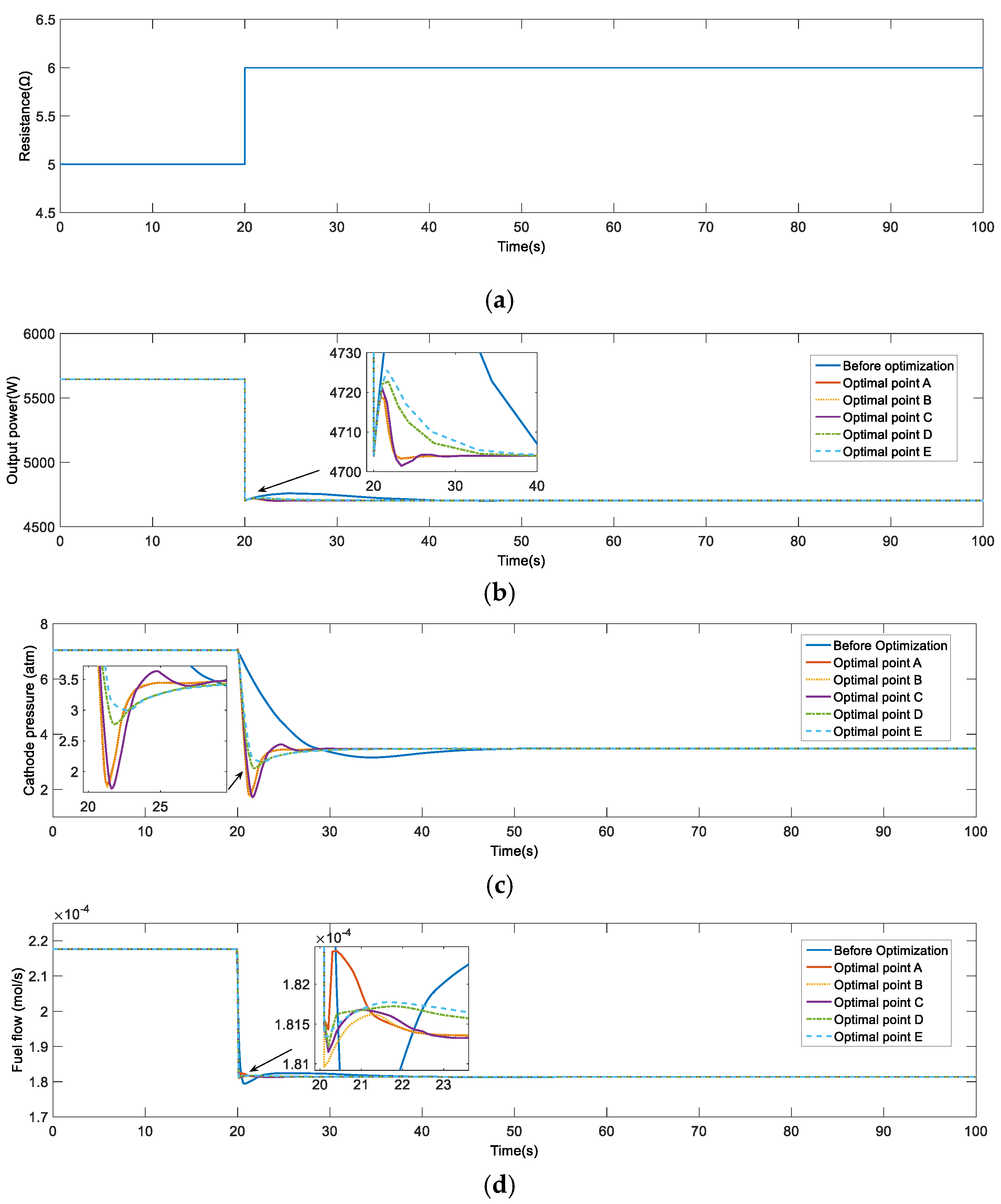
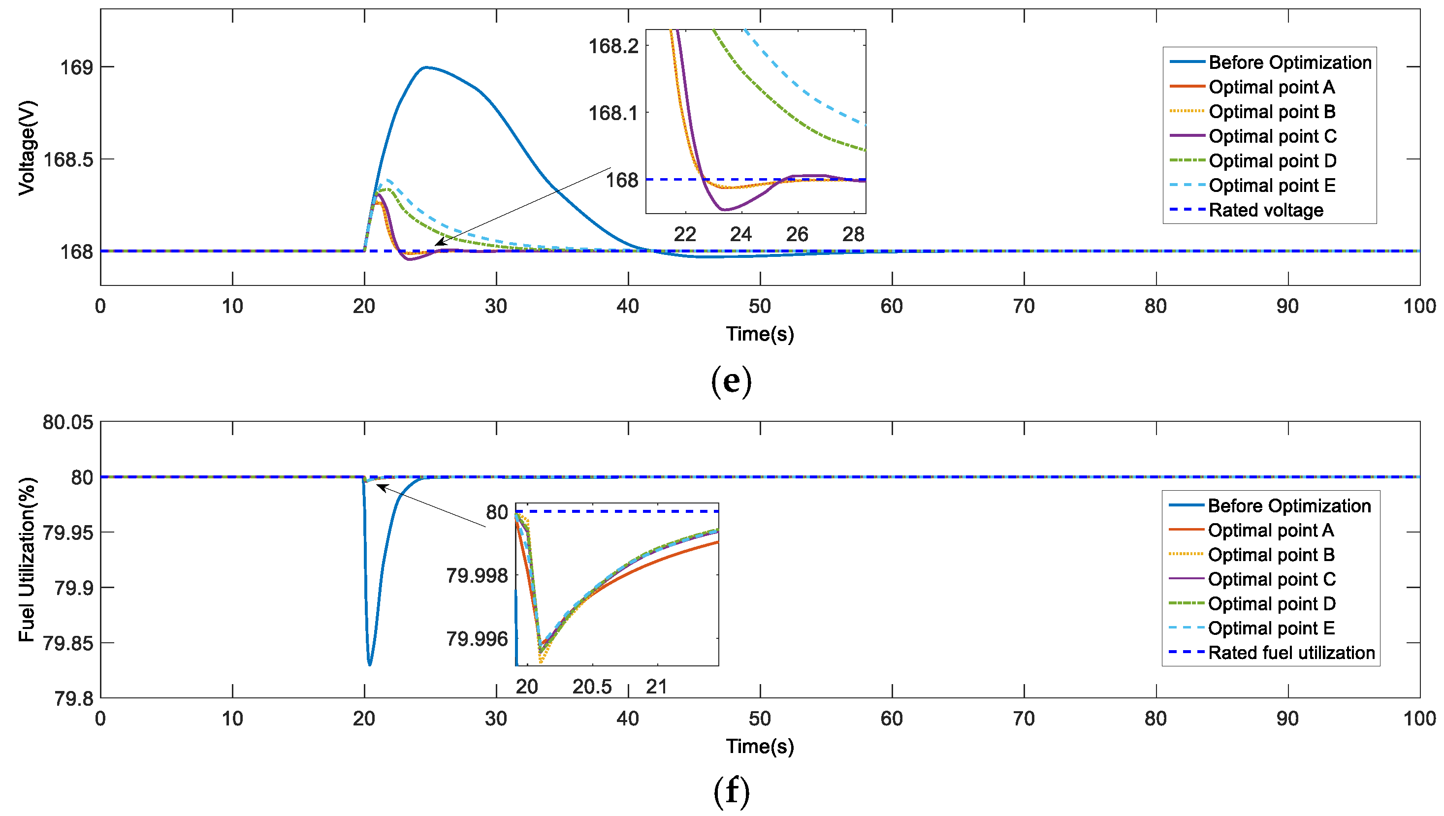
5. Results and Discussion

In this section, to analyze the control performance of the five sets of optimal control parameters and the initial control parameters, a simulation was performed based on the linearized model implemented, and the results were compared and discussed.

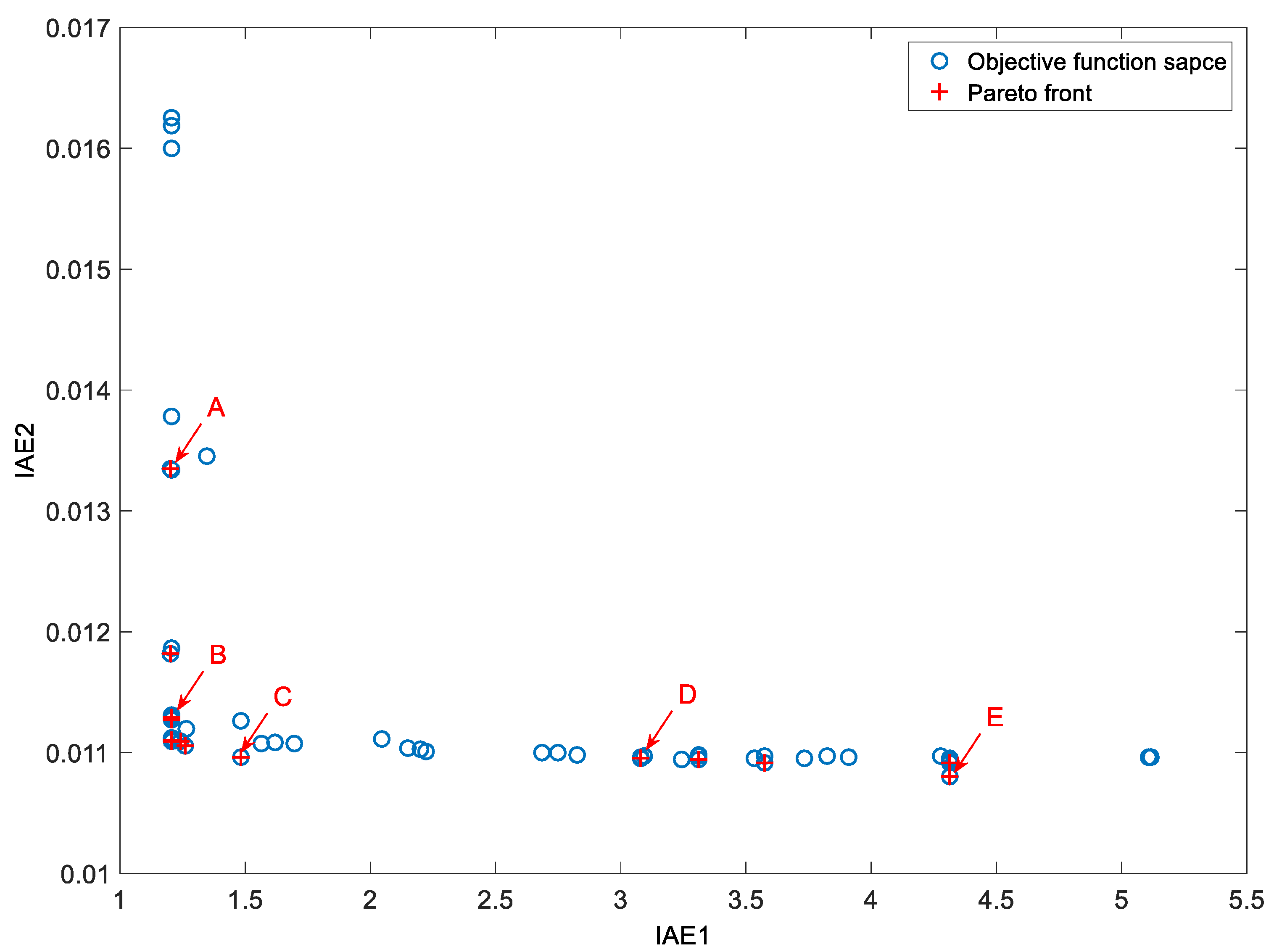
5.1. Comparison of the Optimal Points

In this part, a step signal was added to the load resistance, and the disturbance responses of the controllers on the five optimal points and the original controller were compared. The best optimal points were chosen based on the comparison results.

5.1.1. Simulation Results

During the simulation process, a step signal was added to the load resistance to make it change from 5 Ω to 6 Ω at 20 s, while the reference values of Vout and FU were 168 V and 80%, respectively. The disturbance responses of the output power Pout, the output voltage, the fuel utilization, the fuel flow, and the cathode pressure are shown in Figure 8, and detailed data from the simulation are shown in Table 2.

5.1.2. Discussion

From the simulation results, we can observe that compared to the initial controller before optimization, the controllers tuned to the five optimal points all had better control performance.
In Figure 8b, the controllers on the five optimal points all had faster dynamic responses on Pout compared to the initial controller. At optimal point A, the speed of the dynamic response was the fastest, while optimal point E possessed the slowest dynamic response. In Figure 8c,d, the controllers on the five optimal points all had faster control effects on Pc and mH2.
In Figure 8e, it is clear that the control performance of Vout could be dramatically improved by applying the controllers on the five optimal points, and the settling time and IAE of the output voltage gradually increased from optimal point A to E, while the optimal point C possessed the biggest overshoot among all the optimal points (0.0211%). In Figure 8f, both the settling time and IAE of the response of FU on the five optimal points were better than those before optimization. Among all of the optimal points, the controller on point A possessed the longest settling time (1.225 s), while the settling time for the controller before optimization was 4.832 s. In addition, the controller on optimal point E possessed the best control performance with the shortest settling time, 0.062 3 s, and the lowest IAE, 0.0017.
In conclusion, the controllers on the five optimal points all had a smaller overshoot, lower settling times, and a lower IAE than the initial controller. Based on the simulation results, the control parameters on optimal point D were chosen as the best solution in order to reduce the control action and improve the control performance of both the output voltage and fuel utilization.
Additionally, there were some defects in the optimization process. Compared to the improved NSGA-II we applied in this paper, the NSGA-III proposed by Deb and Jain [33] in 2014 is more proper for an MOP with a Pareto front, whose objective values may have a different scale. Moreover, the population size and execution times applied were the default values in the Matlab Optimization Toolbox, which could be optimized to save on optimization time.

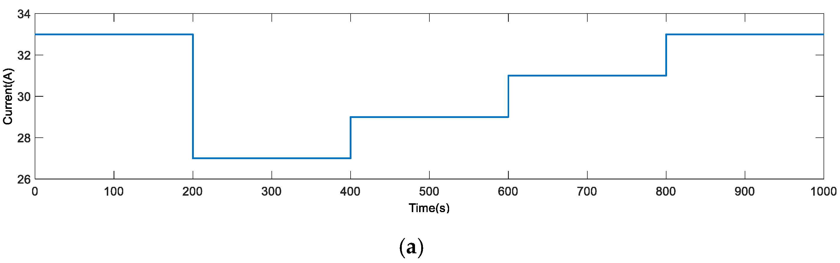
5.2. Continuous Disturbance Response Simulation

In this part, continuous step signals were added to the load resistance and the current to simulate the realistic working conditions of an SOFC. The disturbance responses of the optimal controller based on optimal point D and the original controller were compared, and conclusions were drawn based on the simulation results.

5.2.1. Resistance Disturbance Response Simulation

During the simulation process, a continuous step signal was added to the load resistance to make it change from 5 Ω to 5.5 Ω, 6 Ω, 6.5 Ω, and 5 Ω at 200 s, 400 s, 600 s, and 800 s, respectively. The reference values of Vout and FU were kept at 168 V and 80%, respectively. The disturbance responses of the output power Pout, the output voltage, the fuel utilization, the fuel flow, and the cathode pressure are shown in Figure 9, and detailed data from the simulation are shown in Table 3.

5.2.2. Current Disturbance Response Simulation

During the simulation process, a continuous step signal was added to the current to make it change from 33 A to 27 A, 29 A, 31 A, and 33 A at 200 s, 400 s, 600 s, and 800 s, respectively. The reference values of Vout and FU were kept at 168 V and 80%, respectively. The disturbance responses of the output power Pout, the output voltage, the fuel utilization, the fuel flow, and the cathode pressure are shown in Figure 10, and detailed data from the simulation are shown in Table 4.

5.2.3. Discussion

From the simulation results, it is evident that compared to the original controller, the optimal controller based on the controller parameters on optimal point D had better control performance.
In Figure 9b and Figure 10b, the step responses of the optimal controller possessed faster dynamic responses than the original one, which led to fewer fluctuations in the output power. Figure 9c,d and Figure 10c,d, also illustrate that the optimal controller had more rapid dynamic responses to cathode pressure and fuel flow, which permitted faster control action in the controller.
From Figure 9e and Figure 10e, it is clear that the control performance of the optimal controller was much better than the original controller from the perspective of the overshoot and settling time. The overshoot of all of the disturbance responses of the optimal controller was 0, whereas the original controller had a slight overshoot. As for the settling time, the settling time of the optimal controller under resistance disturbance varied from 8.5 s to 16.4 s, while that of the original controller under resistance disturbance varied from 18.1 s to 46.2 s. In addition, the settling time of the optimal controller under current disturbance varied from 12.1 s to 17.3 s, while that of the original controller under resistance disturbance varied from 37.6 s to 50.3 s.
In Figure 9f and Figure 10f, although the overshoot of both the original controller and optimal controller was 0, the settling time of the optimal controller was much shorter due to the rapid control action. The settling time of the optimal controller under resistance disturbance varied from 1.1 s to 2.4 s, and as for the original controller, it varied from 4.8 s to 6.8 s. The settling time of the optimal controller under current disturbance varied from 1.8 s to 2.2 s, and the original controller varied from 5.2 s to 6.7 s.
In conclusion, from the simulation results of the continuous disturbance response, it is clear that the optimal controller on optimal point D had the merits of stability, a smaller overshoot, and reduced settling time, and consequently, it is the ideal controller for the SOFC model under consideration.

6. Conclusions

An SOFC is an efficient energy conversion device that has been widely used. To deal with the characteristics of couplings of multivariables, nonlinearity of the model, and frequent load disturbances, this paper employed a GA-based optimization algorithm to find the optimal parameters for the PID controllers of an SOFC. In this paper, a 3 × 2 MIMO system was identified based on the SOFC model, and two PID controllers were designed to separately control Vout and FU. Then, the optimization objectives were designed, and a GA was applied for multiobjective optimizations of the controller parameters for the two controllers. Finally, a set of optimal points on the Pareto front were found, and the corresponding control parameters of the five points were applied to control the linearized SOFC model. The results showed that the controller parameters at the five optimal points resulted in better control performance compared to before optimization in terms of the IAE, the overshoot, and the settling time. The parameters on optimal point D were considered to be the best for their smooth control action. Therefore, PID controllers with the controller parameters on optimal point D are an ideal choice for SOFC control.

Author Contributions

All authors collectively conceived of the research and carried out the analysis. Y.Q. and Q.H. led the simulations and paper writing, with contributions and supervision from L.S., G.Z. and S.N.

Funding

This research was funded by the National Natural Science Foundation of China under Grant 51806034; the Natural Science Foundation of Jiangsu Province, China, under Grant BK20170686; the open funding of the Jiangsu Province Key Lab of Aerospace Power System, Nanjing University of Aeronautics and Astronautics, under Grant CEPE2018010; and the open funding of the state key lab of Engines, Tianjin University.

Conflicts of Interest

The authors declare no conflicts of interest.

Nomenclature

Nomenclature
Aarea (m2)
aConstant material resistance (Ω∙m)
bConstant material resistance (K)
CHeat capacity [J/(mol∙K)]
EReversible potential (V)
FFaraday constant, 96487 (C/mol)
hHeat transfer coefficient [W/(m2·K)]
I, iCurrent (A)
i0Exchange current (A)
MMole flow rate (mol/s)
mMass (kg)
NNumber of cells in the stack
P, pPressure (atm)
qEnergy (J)
RGas constant, 8.3143 J/(mol·K), or resistance (Ω)
TTemperature (K)
VVoltage (V)
xMole fraction
δLength/thickness (m)
εEmissivity
σStefan–Boltzmann constant, 5.67 × 10⁻⁸ (W·m−2·K−4.)
Superscripts and subscripts
actActivation
airConditions for air
anAnode
annAnnulus of the cell
ASTAir supply tube
caCathode
cellConditions for individual cell
chemChemical
conConcentration
convConvective
eleElectticity
flowFlow heat exchange
fuelConditions for fuel
genGenerated
H2Hydrogen
H2OWater
inConditions of input/inlet
innerInner conditions
itcInterconnection between cells
netNet values
O2Oxygen
ohmOhmic
outConditions of output/outlet
outerOuter conditions
radRadiation
refReference value

References

  1. Sun, L.; Shen, J.; Hua, Q.; Lee, K. Data-driven oxygen excess ratio control for proton exchange membrane fuel cell. Appl. Energy 2018, 231, 866–875. [Google Scholar] [CrossRef]
  2. Lou, Y.; Liao, Z.; Sun, J.; Jiang, B.; Wang, J.; Yang, Y. A novel two-step method to design inter-plant hydrogen network. Int. J. Hydrog. Energy 2019, 44, 5686–5695. [Google Scholar] [CrossRef]
  3. Sun, L.; Wu, G.; Xue, Y.; Shen, J.; Li, D.; Lee, K.Y. Coordinated control strategies for fuel cell power plant in a microgrid. IEEE Trans. Energy Convers. 2017, 33, 1–9. [Google Scholar] [CrossRef]
  4. Sun, L.; Hua, Q.; Shen, J.; Xue, Y.; Li, D.; Lee, K. A combined voltage control strategy for fuel cell. Sustainability 2017, 9, 1517. [Google Scholar] [CrossRef]
  5. Wu, L.; Sun, L.; Shen, J.; Hua, Q. Multiple model predictive hybrid feedforward control of fuel cell power generation system. Sustainability 2018, 10, 437. [Google Scholar] [CrossRef]
  6. Wei, L.; Shen, Y.; Liao, Z.; Sun, J.; Jiang, B.; Wang, J.; Yang, Y. Balancing between risk and profit in refinery hydrogen networks: A Worst-Case Conditional Value-at-Risk approach. Chem. Eng. Res. Des. 2019, 146, 201–210. [Google Scholar] [CrossRef]
  7. Rao, M.; Fernandes, A.; Pronk, P.; Aravind, P.V. Design, modelling and techno-economic analysis of a solid oxide fuel cell-gas turbine system with CO2 capture fueled by gases from steel industry. Appl. Therm. Eng. 2019, 148, 1258–1270. [Google Scholar] [CrossRef]
  8. Xia, C.; Qiao, Z.; Feng, C.; Kim, J.-S.; Wang, B.; Zhu, B. Study on Zinc Oxide-Based Electrolytes in Low-Temperature Solid Oxide Fuel Cells. Materials 2018, 11, 40. [Google Scholar] [CrossRef]
  9. Wang, W.; Qu, J.; Julião, P.S.B.; Shao, Z. Recent Advances in the Development of Anode Materials for Solid Oxide Fuel Cells Utilizing Liquid Oxygenated Hydrocarbon Fuels: A Mini Review. Energy Technol. 2019, 7, 33–44. [Google Scholar] [CrossRef]
  10. Li, Y.H.; Rajakaruna, S.; Choi, S.S. Control of a Solid Oxide Fuel Cell Power Plant in a Grid-Connected System. IEEE Trans. Energy Convers. 2007, 22, 405–413. [Google Scholar] [CrossRef]
  11. Jacobsen, L.T.; Spivey, B.J.; Hedengren, J.D. Model predictive control with a rigorous model of a Solid Oxide Fuel Cell. In Proceedings of the 2013 American Control Conference, Washington, DC, USA, 17–19 June 2013; p. 3741. [Google Scholar]
  12. Pohjoranta, A.; Halinen, M.; Pennanen, J.; Kiviaho, J. Model predictive control of the solid oxide fuel cell stack temperature with models based on experimental data. J. Power Sources 2015, 277, 239–250. [Google Scholar] [CrossRef]
  13. Oh, S.-R.; Sun, J.; Dobbs, H.; King, J. Model Predictive Control for Power and Thermal Management of an Integrated Solid Oxide Fuel Cell and Turbocharger System. IEEE Trans. Control Syst. Technol. Control Syst. Technol. 2014, 22, 911–920. [Google Scholar]
  14. Qin, Y.; Sun, L.; Hua, Q.; Liu, P. A Fuzzy Adaptive PID Controller Design for Fuel Cell Power Plant. Sustainability 2018, 10, 2438. [Google Scholar] [CrossRef]
  15. Sakhare, A.R.; Davari, A.; Feliachi, A. Control of stand alone solid oxide fuel cell using fuzzy logic. In Proceedings of the 35th Southeastern Symposium on System Theory, Morgantown, WV, USA, 18 March 2003; p. 473. [Google Scholar]
  16. Ji, N.; Xu, D.; Liu, F. A novel adaptive neural network constrained control for solid oxide fuel cells via dynamic anti-windup. Neurocomputing 2016, 214, 134–142. [Google Scholar] [CrossRef]
  17. Qin, Y.; Sun, L.; Hua, Q. Environmental health oriented optimal temperature control for refrigeration systems based on a fruit fly intelligent algorithm. Int. J. Environ. Res. Public Health 2018, 15, 2865. [Google Scholar] [CrossRef] [PubMed]
  18. Zamani, M.; Karimi-Ghartemani, M.; Sadati, N.; Parniani, M. Design of a fractional order PID controller for an AVR using particle swarm optimization. Control Eng. Pract. 2009, 17, 1380–1387. [Google Scholar] [CrossRef]
  19. Elbayomy, K.M.; Zongxia, J.; Huaqing, Z. PID Controller Optimization by GA and Its Performances on the Electro-hydraulic Servo Control System. Chin. J. Aeronaut. 2008, 21, 378–384. [Google Scholar] [CrossRef] [Green Version]
  20. Sun, L.; Shen, J.; Hua, Q.; Xue, Y.; Li, D.; Lee, K.Y. Multi-objective optimization for advanced superheater steam temperature control in a 300 MW power plant. Appl. Energy 2017, 208, 592–606. [Google Scholar] [CrossRef]
  21. Wang, P.; Yan, X.; Zhao, F. Multi-objective optimization of control parameters for a pressurized water reactor pressurizer using a genetic algorithm. Ann. Nucl. Energy 2019, 124, 9–20. [Google Scholar] [CrossRef]
  22. Huang, J.; Liu, Y.; Liu, M.; Cao, M.; Yan, Q. Multi-Objective Optimization Control of Distributed Electric Drive Vehicles Based on Optimal Torque Distribution. IEEE Access 2019, 7, 16377–16394. [Google Scholar] [CrossRef]
  23. Banos, R.; Manzano-Agugliaro, F.; Montoya, F.; Gil, C.; Alcayde, A.; Gómez, J. Optimization methods applied to renewable and sustainable energy: A review. Renew. Sustain. Energy Rev. 2011, 15, 1753–1766. [Google Scholar] [CrossRef]
  24. Chan, S.H.; Low, C.F.; Ding, O.L. Energy and exergy analysis of simple solid-oxide fuel-cell power systems. J. Power Sources 2002, 103, 188–200. [Google Scholar] [CrossRef]
  25. Hatsopoulos, G.N.; Keenan, J.H. Principles of General Thermodynamics; R. E. Krieger Pub. Co.: Huntington, NY, USA, 1981. [Google Scholar]
  26. Wang, C.; Nehrir, M.H. A Physically Based Dynamic Model for Solid Oxide Fuel Cells. IEEE Trans. Energy Convers. 2008, 22, 887–897. [Google Scholar] [CrossRef]
  27. Skogestad, S.; Postlethwaite, I. Multivariable Feedback Control: Analysis and Design; John Wiley: Chichester, UK; Hoboken, NJ, USA, 2005. [Google Scholar]
  28. Dhieb, Y.; Yaich, M.; Guermazi, A.; Ghariani, M. PID Controller Tuning using Ant Colony Optimization for Induction Motor. J. Electr. Syst. 2019, 15, 133–141. [Google Scholar]
  29. Holland, J.H. Adaptation in Natural and Artificial Systems; University of Michigan Press: Ann Arbor, MI, USA, 1975. [Google Scholar]
  30. Srinivas, N.; Deb, K. Muiltiobjective optimization using nondominated sorting in genetic algorithms. Evol. Comput. 1994, 2, 221–248. [Google Scholar] [CrossRef]
  31. Deb, K.; Agrawal, S.; Pratap, A.; Meyarivan, T. A Fast Elitist Non-Dominated Sorting Genetic Algorithm for Multi-Objective Optimization: NSGA-II; Schoenauer, M., Deb, K., Rudolph, G., Yao, X., Lutton, E., Merelo, J.J., Schwefel, H.-P., Eds.; Parallel Problem Solving from Nature PPSN VI; Springer: Berlin/Heidelberg, Germany, 2000; pp. 849–858. [Google Scholar]
  32. Nagarkar, M.P.; Vikhe Patil, G.J.; Bhalerao, Y.J.; Zaware Patil, R.N. GA-based multi-objective optimization of active nonlinear quarter car suspension system—PID and fuzzy logic control. Int. J. Mech. Mater. Eng. 2018, 13, 10. [Google Scholar] [CrossRef]
  33. Deb, K.; Jain, H. An Evolutionary Many-Objective Optimization Algorithm Using Reference-Point-Based Nondominated Sorting Approach, Part I: Solving Problems with Box Constraints. IEEE Trans. Evol. Comput. 2014, 18, 577–601. [Google Scholar] [CrossRef]
Figure 1. A structural diagram of a solid oxide fuel cell (SOFC).
Sustainability 11 03290 g001
Figure 2. Step response curves of the identified model and the original model. (a) Comparison of step response curves of G11; (b) Comparison of step response curves of G21; (c) Comparison of step response curves of G12; (e) Comparison of step response curves of G22; (e) Comparison of step response curves of d1; (f) Comparison of step response curves of d2.
Sustainability 11 03290 g002aSustainability 11 03290 g002b
Figure 3. Structure of the control system.
Sustainability 11 03290 g003
Figure 4. Schematic diagram of a Pareto front.
Sustainability 11 03290 g004
Figure 5. Flow chart of the improved nondominated sorting genetic algorithm (NSGA)-II.
Sustainability 11 03290 g005
Figure 6. The distribution of the final generation in the objective function space.
Sustainability 11 03290 g006
Figure 7. The trend lines of the objective functions: (a) The trend line of IAE1; (b) the trend line of IAE2.
Sustainability 11 03290 g007
Figure 8. Simulation results of a step response: (a) Step input of R; (b) disturbance response of Pout; (c) disturbance response of Pc; (d) disturbance response of mH2; (e) disturbance response of Vout; (f) disturbance response of FU.
Sustainability 11 03290 g008aSustainability 11 03290 g008b
Figure 9. Simulation results of a continuous step response: (a) Step input of R; (b) disturbance response of Pout; (c) disturbance response of Pc; (d) disturbance response of mH2; (e) disturbance response of Vout; (f) disturbance response of FU.
Sustainability 11 03290 g009aSustainability 11 03290 g009b
Figure 10. Simulation results of a continuous step response: (a) Step input of the current; (b) disturbance response of Pout; (c) disturbance response of Pc; (d) disturbance response of mH2; (e) disturbance response of Vout; (f) disturbance response of FU.
Sustainability 11 03290 g010aSustainability 11 03290 g010b
Table 1. The value of the control parameters and objective functions at the five optimal points.
Control ParametersABCDE
kp1−0.00753−0.00666−0.00708−0.00677−0.00733
ki1−0.00981−0.00983−0.00985−0.00999−0.00998
kd18.18 × 10−57.68 × 10−55.40 × 10−56.58 × 10−55.88 × 10−5
Td156.0111955.9675268.611953.981848.92057
kp29.9503849.9533417.9952759.5061238.360098
ki29.9776869.9751389.2003532.3422231.672613
kd2−0.92397−0.90781−0.51078−0.63197−0.50791
Td269.3071269.3229951.5797469.1891863.97332
IAE11.2031.2051.4813.0814.313
IAE20.01340.01130.01110.0110.0108
Table 2. Detailed data from the simulation results.
Output VariablesIndexBefore OptimizationOptimal Point AOptimal Point BOptimal Point COptimal Point DOptimal Point E
Output VoltageOvershoot (%)0.02270.01130.01110.021100
Settling time (s)38.2314.2934.3564.90310.86517.108
IAE111.75060.28970.29240.34950.89722.0206
Fuel UtilizationOvershoot (%)000000
Settling time (s)4.8321.2250.9270.09370.06520.0623
IAE20.26110.00370.00280.00250.00180.0017
Table 3. Detailed data from the simulation results.
Output VariablesNumberOptimal ControllerOriginal Controller
Overshoot (%)Settling Time (s)Overshoot (%)Settling Time (s)
Output Voltage109.60.01230.3
209.30.00724.5
308.5018.1
4016.40.06046.2
Fuel Utilization101.405.4
201.505.2
301.104.8
402.406.8
Table 4. Detailed data from the simulation results.
Output VariablesNumberOptimal ControllerOriginal Controller
Overshoot (%)Settling Time (s)Overshoot (%)Settling Time (s)
Output Voltage1017.30.01837.6
2011.90.00938.8
3012.70.01240.5
4012.10.01550.3
Fuel utilization102.206.5
201.505.6
301.405.2
401.806.7

