A Multi-Step Approach Framework for Freight Forecasting of River-Sea Direct Transport without Direct Historical Data

Abstract

The freight forecasting of river-sea direct transport (RSDT) is crucial for the policy making of river-sea transportation facilities and the decision-making of relevant port and shipping companies. This paper develops a multi-step approach framework for freight volume forecasting of RSDT in the case that direct historical data are not available. First, we collect publicly available shipping data, including ship traffic flow, speed limit of each navigation channel, free-flow running time, channel length, channel capacity, etc. The origin–destination (O–D) matrix estimation method is then used to obtain the matrix of historical freight volumes among all O–D pairs based on these data. Next, the future total freight volumes among these O–D pairs are forecasted by using the gray prediction model, and the sharing rate of RSDT is estimated by using the logit model. The freight volume of RSDT is thus determined. The effectiveness of the proposed approach is validated by forecasting the RSDT freight volume on a shipping route of China.

1. Introduction

River-sea direct transport (RSDT) is a kind of sustainable transportation mode directly connecting river and sea, which uses river-sea ships for direct transport without transshipment. It has been reported that the introduction of RSDT mode is able to reduce the total shipping cost by more than 8% comparing to the reduction of about 2% by the river-sea combined mode [1]. Besides, the RSDT mode is able to reduce shipping time, fuel consumptions and carbon emissions.

Due to various realistic restrictions such as river conditions and ship types, the RSDT mode has not been well-developed [2]. Many researchers have studied the design and optimization of river-sea ship [1,3,4,5,6,7], the function model [8,9] and the characteristics and strength analysis [10,11,12,13,14] of RSDT. Cinquini et al. [4] addressed the shape optimization problem of an innovative river-sea ship designed to achieve an improved dynamic behavior in both river and sea navigation conditions. Wu et al. [11] investigated the ultimate strength of a river-sea ship under combined action of bending and torsion by the means of numerical and experimental research. Guo et al. [12] carried out a hydrodynamic analysis of river-sea container ships under specific routes based on the three-dimensional potential flow theory, which placed a foundation for fatigue assessment of new inland-ocean container ships. By investigating the characteristics and structure of the river-sea combined transport, Egorov and Tonyuk [13] provided the optimal propulsion system selection for combined ships and presented the comparison results of fuel efficiency at different cruising speeds.

Nowadays, as China’s coastal economy and inland economy enter a new era of synergistic development, the traditional shipping transport mode is facing new challenges of transformation and upgrading. RSDT, as an important way of deepening the supply-side structural reform of transportation, is attracting more and more attention. Compared with similar sea-going ship, this RSDT ship leads to the reduction of about 10% in the total shipping cost, the increase of about 13% in the load capacity and the reduction of about 12% in the energy consumption. This RSDT model is in line with the green and low-carbon development trend [15,16,17,18,19] nowadays. China plans to establish a safe, efficient and green direct transportation system by 2030 and to complete the construction of the RSDT system from the Yangtze River and Yangtze River delta region to Ningbo-Zhoushan port and Shanghai-Yangshan port in 2020 [20]. In order to achieve this goal, it is very important to forecast the RSDT freight demand effectively.

The freight volume of RSDT is one of the important indicators reflecting the demand of direct transport, and it is also critical for the local government to determine the scale of infrastructure construction and make relevant shipping transport policies. Moreover, shipping companies need to establish development and operation strategies on the basis of certain demands of river-sea freight volumes. Therefore, forecasting RSDT freight volume effectively is of great significance for the RSDT development.

Research on freight volume forecasting in different industries has been reported extensively [21,22,23,24,25,26,27,28,29,30]. Rashed et al. [28] developed a three-step approach by combining the autoregressive distributed lag model with economic scenarios to capture the potential impact of specific risks, modeling and forecasting the demand of container throughput. Ruiz-Aguilar et al. [29] proposed a novel methodology based on a three-step procedure in order to better predict inspections volume, integrating a clustering technique and a hybrid prediction model. Traditional freight volume forecasting methods make forecasts usually based on historical data. We can use these methods to forecast the freight volume in the future if we have the historical freight volumes between ports of origin (O) and ports of destination (D), which is called usually as the origin–destination (O–D) matrix of historical freight volumes. Unfortunately, as a new transport mode in China, RSDT is still in its infancy of entering the market, for which historical data are rare and difficult to obtain. Therefore, it is infeasible to use the existing forecasting method directly to forecast the RSDT freight volume. Unfortunately, there is no relevant research on RSDT freight forecasting so far.

This paper thus aims to develop an effective method for RSDT freight volume forecasting when direct historical data are not available. The RSDT freight in a port consists of ingoing and outgoing freights. The goal of RSDT freight volume forecasting is to obtain the summation of ingoing and outgoing freight volumes between a specified O–D pair of RSDT in the future year. Due to the unavailability of the O–D matrix of historical RSDT freight volumes in China, this research thus investigates how to forecast RSDT freight volume based on publicly available indirect shipping data and effective methods in the absence of such direct data. Available indirect shipping data usually includes ship traffic flow, speed limit of each navigation channel, free-flow running time, channel length, channel capacity, etc.

This paper contributes to the literature by developing a multi-step approach framework for RSDT freight volume forecasting. To the best of the authors’ knowledge, it is the first study of investigating RSDT freight forecasting in the literature. The proposed methodology is capable of making effective freight volume forecasting in the case that direct historical freight data are unavailable by combining OD matrix estimation, gray prediction and logit model.

2. A Multi-Step Approach Framework for RSDT Freight Volume Forecasting

2.1. Overview of the Multi-Step Approach Framework

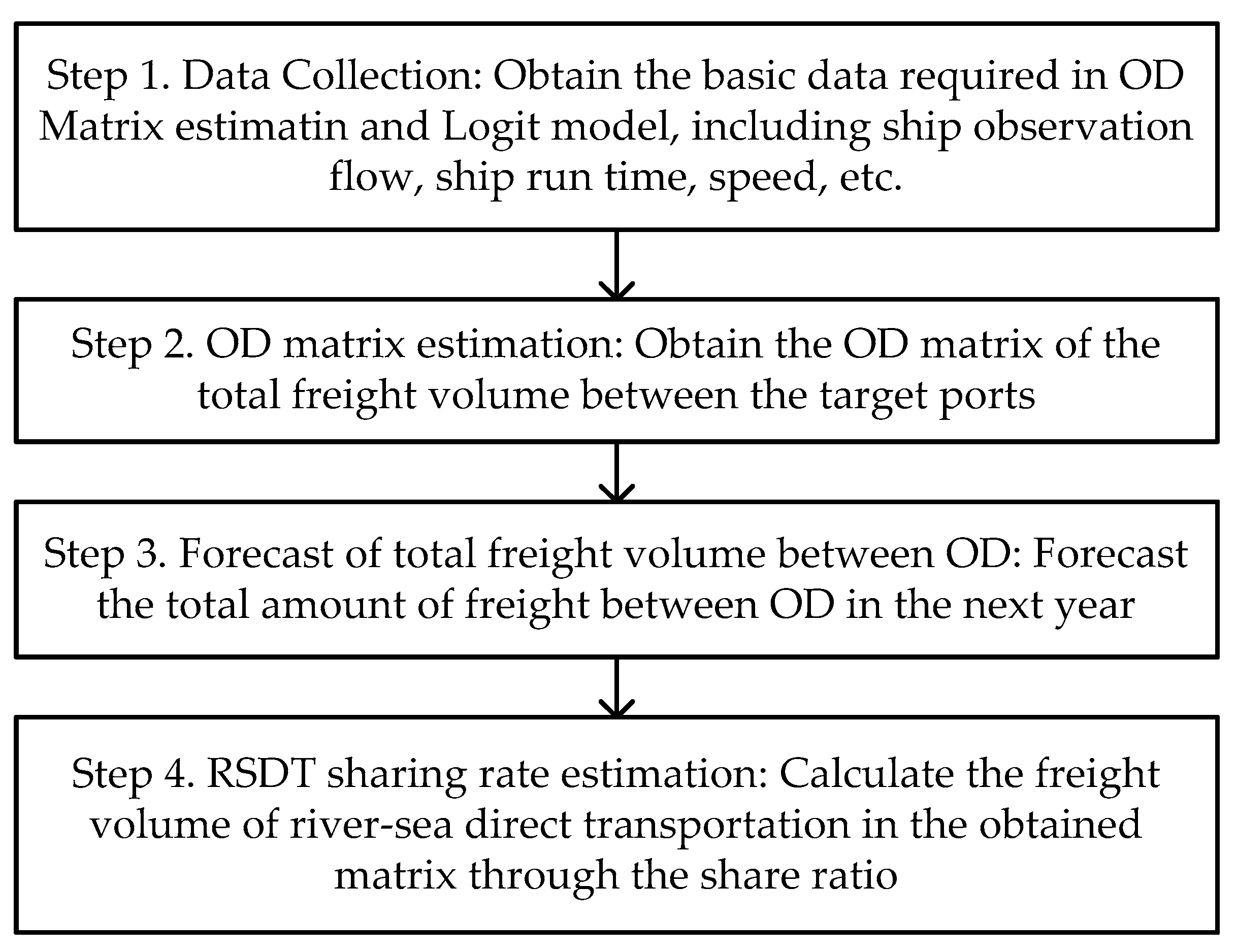
This research proposes a multi-step approach framework for the RSDT freight volume forecasting, as shown in Figure 1. Since the O–D matrix of historical RSDT freight volumes is not available, a natural starting point of our methodology is to first observe and collect publicly available shipping-related data of specific routes, such as shipping transport-related traffic flow, speed limit of each navigation channel, free-flow running time, channel length and channel capacity. On the basis of these data, we then use the O–D matrix estimation method to obtain the O–D matrix of historical RSDT freight volumes among all O–D pairs. Next, the gray prediction method is used to predict the total freight volume between the specified O–D pair in future years, which contains the total freight volume of all shipping transport modes, including river-sea combined transport, river-sea push barge transport and river-sea direct transport. Finally, the logit model is adopted to estimate the proportion of RSDT (i.e., the sharing rate) in total freight volume between this O–D pair, so as to obtain the forecast of RSDT freight volume. Based on the above descriptions, the approach framework involves four steps: Data collection, O–D matrix estimation, forecast of total freight volume between all O–D pairs and RSDT sharing rate estimation. These steps are detailed in Section 2.2, Section 2.3, Section 2.4 and Section 2.5.

2.2. Data Collection

Data collection is to collect the data required in the forecasting process. In the four steps shown in Figure 1, the future total freight forecast is generated based on the O–D matrix estimation. Therefore, only the data required in the O–D matrix estimation and the logit model need to be collected.

2.2.1. Data Required in O–D Matrix Estimation

The O–D matrix estimation, as detailed in Section 2.3, is a process of estimating the O–D matrix based on publicly available data (e.g., traffic flow). In this process, the required data include shipping transport-related traffic flow, speed limit of each navigation channel, free-flow running time, channel length, channel capacity and an initial O–D matrix. Among them, the first five can be observed on the website http://www.shipxy.com/, which uses more than 60 satellites and 2500 automatic identification system base stations to provide Internet-based information and positioning services of vessels among more than 3000 ports worldwide. The historical O–D matrix is usually used as the initial O–D matrix if the historical matrix is available. In the absence of the historical O–D matrix, this research used the matrix with a diagonal value of 0 and the remainder of 1 as the initial O–D matrix.

2.2.2. Data Required in Logit Model

The logit model, as detailed in Section 2.5, is a commonly used method for determining the sharing rates of different transport modes. The utility function is the decisive factor influencing the choice of a transport mode, which will be formulated in Formula (7). We needed to determine the factors that influence the cargo owner’s choice of a particular mode of transport first. Based on these influencing factors, the required data of the utility function can be divided into two parts. The first part is the proportions of different influencing factors, which can be determined by analytic hierarchy process [31], since it is a classical method for determining the weight of factors. The second part is the utility values, which indicates the decision criteria of shippers for different factors. We rated the factors based on their gradings given by shipping practitioners and researchers.

2.3. O–D Matrix Estimation

The O–D matrix estimation method aims at estimating the freight volumes between O–D pairs by traffic flow volumes, which is widely used in highway traffic forecasting. This research applied the O–D matrix estimation method to estimate the historical freight volumes of shipping transport among all O–D pairs, since the forecasting of RSDT freight volume is similar to the forecasting of highway traffic flow. Let $N$ denote the number of ports (indexed by $i$, $j$). There are $M$ route segments (indexed by $a$) between port $i$ and port $j$. The principle of O–D matrix estimation can be expressed by the following formula:

$$V_a = {\displaystyle \sum _i{\displaystyle \sum _j{T}_{ij}}}{p}_{ij}^a,$$

(1)

where $V_a$ is the freight volume of route segment $a$, $T_{ij}$ is the amount of freight from port $i$ to port $j$ and $p_{ij}^a$ is the proportion of the freight passing through segment $a$.

According to Formula (1) above, the estimation of $V_a$ is determined by the total freight volumes among all O–D pairs and their proportions passing through segment $a$. For an actual traffic network, the number of traffic segments $M$ is often much smaller than the number of O–D pairs $N(N-1)$ to be sought. Moreover, the traffic flow of all segments cannot be detected, so the optimal O–D matrix cannot be estimated only by the traffic flow. This means that, due to insufficient information, the linear equations will have multiple sets of feasible solutions. Thus, the problem is transformed into the one of choosing the optimal solution (i.e., the optimal O–D matrix) among the many feasible solutions. This requires some additional information to determine the most realistic O–D matrix. Nguyen [32] first proposed a user equilibrium model to solve the O–D matrix estimation problem, which can be easily implemented by using the Transcad software. TransCAD is a geographic information system (GIS) software product developed by Caliper Corporation, which combines GIS and transportation modeling capabilities in a single platform. It is widely used in transportation planning, travel demand forecasting, design and management.

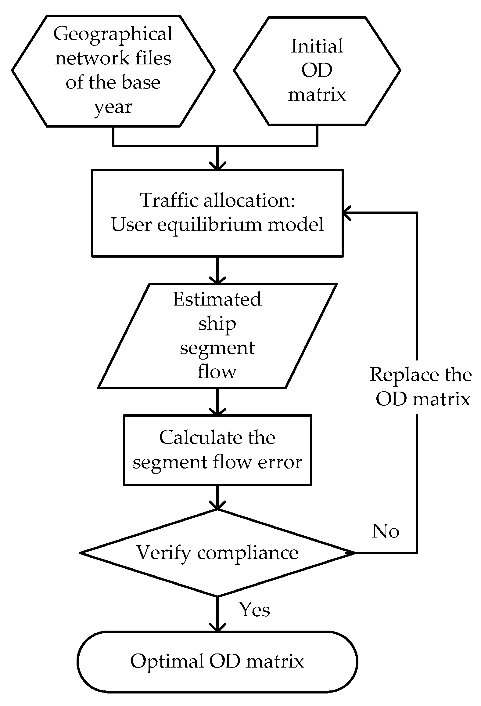
Based on this principle, the flowchart of O–D matrix estimation solved by Transcad software is illustrated in Figure 2. The first operation process was to divide the estimation O–D area and create geographical network files of the base year, where we needed to input basic data, such as ship traffic flow, speed limit of each navigation channel, free-flow running time, channel length and channel capacity, etc. Based on the geographical network files of the base year and the initial O–D matrix, the user equilibrium model [24] was used to allocate the ship traffic. Then, the ship traffic flow of each segment was estimated. The segment flow error was calculated to verify the reliability of the O–D matrix estimation process. If the error was small enough, the optimal matrix was obtained. Otherwise, we needed to replace the O–D matrix and performed the traffic allocation again.

2.4. Forecasting of Total Freight Volumes Among All O–D Pairs

The freight volume matrix obtained by the O–D matrix estimation is the historical freight volume data between ports of all O–D pairs, which is so-called the historical O–D matrix. Next, based on this matrix, we could forecast directly the total freight volumes among all O–D pairs in the future year.

The freight volume forecast between an O–D pair usually depends on the freight volumes in recent years. The available data of historical freight volumes are usually limited and uncertain. The gray prediction model is a forecasting method capable of generating effective forecasts based on a small amount of historical data. There is no need to know the priori characteristics of historical data, and can better maintain the actual situation of the original system. The gray model contains both certain and uncertain information, and predicts the time series-related processes for less data within a certain range. Therefore, this study used the gray prediction model [33] to predict the total freight volumes among all O–D pairs in the future year, in which the posterior ratio $C$ and the probability $P$ of small error were used to test the accuracy of the model.

The gray prediction model is presented as follows:

(1) Assume that the original data sequence is $X^{(0)}=\left\{x^{(0)}(1),x^{(0)}(2),\dots ,x^{(0)}(n)\right\},n\ge 4$;

(2) Generate an accumulation sequence $X^{(1)}=\left\{x^{(1)}(1),x^{(1)}(2),\dots ,x^{(1)}(n)\right\},n\ge 4$ based on $X^{(0)}$, where $x^{(1)}(k) = {\displaystyle \sum _{i=1}^k{x}^{(0)}(i)}, k = 1,2,\dots ,n$.

Take $GM(1,1)$ model for the accumulated sequence. The prediction principle of GM (1,1) model is described next. First, we generate a set of new data series with obvious trend by means of accumulation for a certain data series. We then build a model for prediction according to the growth trend of the new data series. At last, we conduct an inverse calculation by using the method of subtraction to restore the original data series, so as to obtain the prediction results. That is,

$$\frac{d{x}^{(1)}(k)}{dt} + c{x}^{(1)}(k) = u,$$

(2)

where $c$ is the development of gray number, $u$ is the endogenous control gray number. $c$ and $u$ are solved by least squares method:

$${[c,u]}^{\mathrm{T}}=(B^{\mathrm{T}}B{)}^{-1}{B}^{\mathrm{T}}{Y}_n$$

(3)

where $B=\left(\begin{array}{cc}-\frac{1}{2}[x^{(1)}(1)+x^{(1)}(2)]& 1\\ -\frac{1}{2}[x^{(1)}(2)+x^{(1)}(3)]& 1\\ \dots & \dots \\ -\frac{1}{2}[x^{(1)}(n-1)+x^{(1)}(n)]& 1\end{array}\right)$, $Y_n=[x^{(0)}(2),x^{(0)}(3),\dots ,x^{(0)}(n{)]}^{\mathrm{T}}$.

(3) Solving the differential equation, the time response sequence can be obtained as follows:

$${\widehat{X}}^{{}^{(1)}}(k + 1) = (x^{(0)}(1) - \frac{u}{c}{)\mathrm{e}}^{-ck} + \frac{u}{c},$$

(4)

where $k =0,1,2.....,n$.

Since sequence $X^{(1)}$ is a first-order accumulation sequence of $X^{(0)}$, a subtraction of ${\widehat{X}}^{{}^{(1)}}(k+1)$ gives an estimate of $X^{(0)}$. That is,

$${\widehat{X}}^{(0)}(k + 1) = {\widehat{X}}^{ (1)}(k + 1){\widehat{X}}^{(1)}(k) = (1 -{ \mathrm{e}}^{-c}{)(\mathrm{X}}^{(0)}(1) - \frac{u}{c}{)\mathrm{e}}^{-ck}.$$

(5)

In general, there are two criteria to validate the accuracy of the gray prediction model. The first one is the posterior ratio $C$, which is derived by dividing $S_2$ by $S_1$, that is $C = S_1/S_2$. And $S_1$ is the standard deviation of the original time series, $S_2$ is the standard deviation of the forecasting errors. The lower $C$ is, the better the forecasting model is. The other is the probability of small error, which is defined as $P = prob.\left\{\left|e(k) - \overline{\mathrm{e}}\right| < 0.6745S_1\right\}$, $k = 2,3,\dots ,n$, where $e(k) = X^{(0)}(k) - {\widehat{X}}^{(0)}(k)$, $k = 0,1,2.....,n$. $\overline{\mathrm{e}}$ is the mean of forecasting errors. This shows the probability that the relative bias of the forecasting error is lower than 0.6745. The pairs of the forecasting indicators $P$ and $C$ can characterize for grades of forecasting accuracy. The values of $P$ and $C$ for different accuracy grades are defined in the gray prediction model [28], as shown in

Table 1. Accuracy grade of the GM (1,1) model under different values of $C$ and $P$.

Evaluation Index	Accuracy Grade
	Good	Qualified	General	Unqualified
The posterior diff. ratio $C$	<0.35	<0.5	<0.65	>0.65
The small error probability $P$	>0.95	>0.8	>0.7	<0.70

. To achieve a good forecasting performance, $P$ is commonly required to be larger than 0.95.

2.5. RSDT Sharing Rate Estimation

There are three shipping transportation modes in the river and sea transportation, including river-sea combined transport (RSCT), river-sea push barge (RSPB) system and river-sea direct transport (RSDT). The river-sea combined transport (RSCT) uses sea-going vessels and river-inland vessels transporting separately in different channel segments, and transit at particular places or junction ports. The river-sea push barge (RSPB) system implies a river push boat to sail the push barge to the junction port where it, from the sea push boat, continues to the seaport destination. There, the push barge will be unloaded or possibly sailed, again with a river push boat, to the final inland port of destination. The river-sea direct transport (RSDT) uses the river-sea direct ship to transport without transshipment.

The results of the gray prediction model is the total freight volume of the above three modes. In order to obtain the freight volume of RSDT mode, the sharing rate of RSDT needs to be determined. This paper adopts the logit model to obtain the sharing rate of RSDT in the above modes.

The logit model is a widely used effective method for determining the proportions of different categorical outputs, which is thus used to estimate the sharing rate between a single O–D pair. This model can be formulated as follows:

$$P_k = \frac{e^{U(k)}}{{\displaystyle \sum _k^K{e}^{U(k)}}},$$

(6)

$$U(k) = {\displaystyle \sum _{\mathrm{i}=1}^I{w}_i·X_i}(k),$$

(7)

where $P_k$ is the sharing rate of the $k$th transport mode, and $U(k)$ is the utility function of the $k$th transport mode, $k = 1,\dots ,\mathrm{K}$; $w_i$ is the weight of the $i$th influencing factor, and $0\le w_i\le 1$, $i = 1,2,\dots ,\mathrm{I}$; To use the logit model, we needed to obtain the weights of all influencing factors first. This paper used the analytic hierarchy process (AHP)-based process [23] to calculate the weights of these factors. The detail of AHP-based process is described as follows.

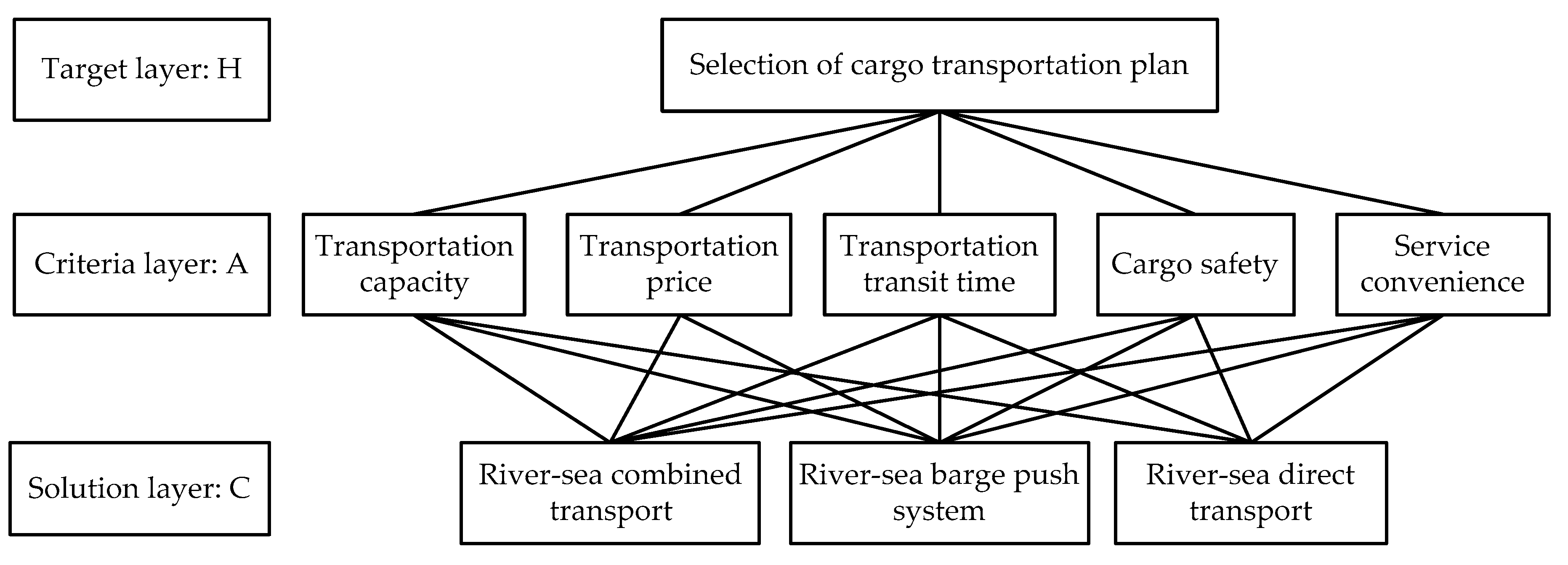
First, we established different levels of element structure diagrams, namely the target layer, the criteria layer and the solution layer. For the target layer $H$, its next criteria layer has $n$ elements $A_1,A_2,\dots ,A_n$. These elements could be transportation capacity, transportation price, transportation transit time, etc. To calculate the weights (denoted by $w_i$) of different influencing factors, we firstly used the pairwise comparison method to get the relative importance of $A_i$ to $H$, and formed the judgment matrix. The judgment matrix is the basic information of the analytic hierarchy process and an important basis for calculating the weight of each element. An example of the judgment matrix of pair-wise comparison factors is shown in

Table 2. Judgment matrix of pair-wise comparison factors.

$H$	$A_1$	$A_2$	…	$A_j$	…	$A_n$
$A_1$	$a_{11}$	$a_{12}$	…	$a_{1j}$	…	$a_{1n}$
$A_2$	$a_{21}$	$a_{22}$	…	$a_{2j}$	…	$a_{2n}$
…	…	…	…	…	…	…
$A_i$	$a_{i1}$	$a_{i2}$	…	$a_{ij}$	…	$a_{in}$
…	…	…	…	…	…	…
$A_n$	$a_{n1}$	$a_{n2}$	…	$a_{nj}$	…	$a_{nn}$

.

In Table 2, $a_{ij}$ represents the relative importance of factor $A_i$ to $A_j$ from the perspective of the judgment criteria $H$. If it is assumed that the weights of the factors $A_1,A_2,\dots ,A_n$ under the criterion $H$ are $w_1,w_2,\dots ,w_n$ respectively, $w = (w_1,w_2,\dots ,w_n{)}^T$, then $a_{ij} = w_i/w_j$ and $a_{ij}$ must satisfy these rules $a_{ii} = 1$, $a_{ij} = 1/a_{ji}$, $a_{ik}{a}_{kj} = a_{ij}$. Matrix $A = \left[\begin{array}{cccc}{a}_{11}& a_{12}& \cdots & a_{1n}\\ a_{21}& a_{22}& \cdots & a_{2n}\\ \cdots & \cdots & \cdots & \cdots \\ a_{n1}& a_{n2}& \cdots & a_{nn}\end{array}\right]$ is a judgment matrix. Then, the square root method was used to calculate the relative weights $w_i$ of different influencing factors. We had $V_i = {\displaystyle \prod _{i=1}^n{a}_{ij}^{\frac{1}{n}}}$, $w_i = V_i/{\displaystyle \sum V_i}$ and ${\displaystyle \sum w_i} = 1$.

The element $w_i$ in the judgment matrix is the numerical scale representing the relative importance of two factors, which is called the judgment scale. It varies from 1 to 9, where ‘1’ signifies the same importance of two factors, and ‘9’ indicates that one factor is much more important than the other.

In order to test the consistency of the judgment matrix, the consistency index $CI = \frac{{\lambda }_{\max } - n}{n - 1}$ was built, where ${\lambda }_{\max } = \frac{1}{n}{\displaystyle \sum _{i=1}^n\frac{{(Aw)}_i}{w_i}}$ was the maximum eigenvalue of the judgment matrix. A matrix is consistent only if ${\lambda }_{\max }>n$. If the index $CI$ is less than 0.1, which is a baseline for consistency, the judgment matrix is considered as consistent.

Next, the utility value $X_i(k)$ was used to indicate the decision criteria of shippers for different factors, which could be determined by expert scoring. Participants from the shipping industry and relevant research communities were investigated to obtain the scoring results. Each factor was evaluated by three grades, 1, 2 and 3. Grade ‘3’ means that the score was high, and grade ‘1’ means that the score was low.

3. Case Study

3.1. Case Route of River-Sea Direct Transport

This paper takes the Ningbo-Zhoushan port to Ma’anshan port route as the case route to forecast the RSDT freight volume. In terms of the total cargo throughput, Ningbo-Zhoushan port is the world’s largest and the first billion-ton port. It locates in the Pan-Yangtze River Delta area of China with excellent natural conditions and is the main port of the Zhoushan River-Sea Intermodal Service Center. A 300,000-ton-class ship can get into and out of the port freely. The super-large ship of 400,000 tons or above can wait for the tide to enter and exit. The Yangtze River Economic Belt has been an important sea passage and has the conditions and foundation for developing river-sea combined transport. The route from Ningbo-Zhoushan port to Ma’anshan port is thus selected as the China’s first RSDT route by relevant authorities. In the following, we referred to Ningbo-Zhoushan port as Ningbo port.

3.2. Results

Based on the approach framework described in Section 2, the forecasting process and results for the case route are described as follows.

3.2.1. Data Collection and Results of O–D Matrix Estimation

We obtained the annual average ship traffic flows between 2011 and 2017 through the Statistical Bulletin on the Development of the Transportation Industry, which are listed in

Table 3. Average ship flow of 2011–2017 (Source: Statistical Bulletin of Transport Industry Development).

Year	2011	2012	2013	2014	2015	2016	2017
Annual average daily ship flow (ship)	638	617	628	656	648	663	703
Annual average hourly ship flow (ship)	26.58	25.7	26.16	27.33	27	27.62	29.2

. It could be seen that the difference in annual average ship flow variation was small. Therefore, we observed and recorded the ship traffic flow in the ports along the case route, based on the website http://www.shipxy.com/, as the basic data of O–D estimation. The observed results are shown in

Table 4. Observed flow at major ports per hour (source: http://www.shipxy.com/).

Port	Anqing	Chizhou	Tongling	Wuhu	Ma’anshan	Jiangsu	Shanghai	Ningbo	Taizhou	Jiujiang
Observed flow (Ship per hour)	4	3.6	4.8	8	9	15	9	6	2	1

. On this basis, the O–D matrix estimation was then carried out. We used the information such as the ship traffic flow and the initial matrix as inputs, and used the user equilibrium model to obtain the ship traffic flow matrix, which is shown in

Table 5. Ship flow matrix of 2011–2017 (unit: Ship per hour).

	Anqing	Chizhou	Tongling	Wuhu	Ma’anshan	Shanghai	Ningbo	Taizhou	Jiangsu	Hefei	Jiujiang
Anqing	0	0.40	0.48	0.27	0.30	0.32	0.42	0.53	0.54	0.56	0.17
Chizhou	0.40	0	0.57	0.23	0.27	0.30	0.43	0.56	0.58	0.59	0.14
Tongling	0.48	0.57	0	0.10	0.19	0.25	0.40	0.56	0.58	0.60	0.09
Wuhu	0.27	0.23	0.10	0	0.38	0.40	0.68	0.94	0.90	0.86	0.09
Ma’anshan	0.30	0.27	0.19	0.38	0	0.44	0.95	1.34	1.16	1.05	0.03
Shanghai	0.32	0.30	0.25	0.40	0.44	0	2.26	2.54	1.68	1.34	0.09
Ningbo	0.42	0.43	0.40	0.68	0.95	2.26	0	2.88	1.46	1.14	0.22
Taizhou	0.53	0.56	0.56	0.94	1.34	2.54	2.88	0	0.78	0.74	0.37
Jiangsu	0.54	0.58	0.58	0.90	1.16	1.68	1.46	0.78	0	0.71	0.42
Hefei	0.56	0.59	0.60	0.86	1.05	1.34	1.14	0.74	0.71	0	0.45
Jiujiang	0.17	0.14	0.09	0.09	0.03	0.09	0.22	0.37	0.42	0.45	0

(unit: Ship/h). To convert the unit in Table 5 to million tons, the average load of one ship was multiplied by the number of hours per year. Therefore, this paper sets the conversion coefficient u, and it was equal to 24 (h/d) × 365 (d/year) × the average load (ton/ship) ÷ 1,000,000. The average loads of one ship from 2011 to 2017 were obtained from the China port Yearbook. The conversion coefficients and the average loads of one ship are shown in

Table 6. Average load and conversion factors of 2011–2017 (Source: China Port Yearbook).

Year	2011	2012	2013	2014	2015	2016	2017
Average load capacity (ton/boat)	1186.35	1279.38	1414.11	1499.34	1642.16	1662.88	1770.00
Conversion factor	1039.24	1120.74	1238.76	1313.42	1438.53	1456.68	1550.52

. Based on these conversion factors, we obtained the total freight O–D matrix shown in

Table 7. Total freight volume matrix of 2017 (unit: 10,000 tons).

	Anqing	Chizhou	Tongling	Wuhu	Ma’anshan	Shanghai	Ningbo	Taizhou	Jiangsu	Hefei	Jiujiang
Anqing	0	7.02	8.41	4.86	5.25	5.61	7.41	9.32	9.64	9.85	3.02
Chizhou	7.02	0	10.11	4.06	4.78	5.32	7.52	9.84	10.19	10.38	2.48
Tongling	8.41	10.11	0	1.77	3.36	4.34	7.04	9.89	10.32	10.55	1.63
Wuhu	4.86	4.06	1.77	0	6.72	7.15	12.01	16.57	15.85	15.19	1.59
Ma’anshan	5.25	4.78	3.36	6.72	0	7.72	16.74	23.63	20.53	18.54	0.5
Shanghai	5.61	5.32	4.34	7.15	7.72	0	39.96	44.95	29.75	23.73	1.6
Ningbo	7.41	7.52	7.04	12.01	16.74	39.96	0	50.93	25.81	20.1	3.86
Taizhou	9.32	9.84	9.89	16.57	23.63	44.95	50.93	0	13.75	13.12	6.54
Jiangsu	9.64	10.19	10.32	15.85	20.53	29.75	25.81	13.75	0	12.54	7.35
Hefei	9.85	10.38	10.55	15.19	18.54	23.73	20.1	13.12	12.54	0	7.91
Jiujiang	3.02	2.48	1.63	1.59	0.5	1.6	3.86	6.54	7.35	7.91	0

.

We could obtain the freight volumes of Shanghai port and Ningbo port to Ma’anshan port in 2011–2017 by repeating the above steps, which are shown in

Table 8. Total freight volumes of Shanghai port and Ningbo port to Ma’anshan port in 2011–2017 (Unit: Million tons).

Year	2011	2012	2013	2014	2015	2016	2017
Shanghai-Ma’anshan	4.53	4.89	5.41	5.73	6.28	6.36	7.72
Ningbo-Ma’anshan	9.83	10.60	11.71	12.42	13.6	13.77	16.74
Total	14.36	15.49	17.12	18.15	19.88	20.13	24.46

.

The Ma’anshan port is the main source of water freight transportation within Anhui Province. After opening up RSDT routes, it has a strong attraction to the freight from its surrounding ports, which we could define as Anhui ports. Assume that the freight between Ningbo port to the ports of Anhui Province (Anhui ports) are transported via Ma’anshan direct route, the maximum amount of waterborne freight transport between 2011 and 2017 that can be obtained under ideal conditions are shown in

Table 9. Total freight volume available at Ma’anshan port in 2011–2017 (unit: Million tons).

Year	2011	2012	2013	2014	2015	2016	2017
Ningbo-Anqing	4.35	4.69	5.19	5.50	6.02	6.10	7.41
Ningbo-Chizhou	4.42	4.76	5.27	5.58	6.11	6.19	7.52
Ningbo-Tongling	4.14	4.46	4.93	5.22	5.72	5.79	7.04
Ningbo-Wuhu	7.05	7.60	8.40	8.91	9.76	9.88	12.01
Ningbo-Ma’anshan	9.83	10.60	11.71	12.42	13.60	13.77	16.74
Total	29.79	32.11	35.50	37.63	41.21	41.73	50.72

.

3.2.2. Results of the Total Freight Volume Forecasting

Based on the historical total freight data of 2011–2017, we obtained the gray prediction model as follows,

$${\widehat{X}}^{{}^{(1)}}(k + 1) = 362.93{\mathrm{e}}^{ 0.0842k} - 333.14.$$

(8)

The estimated value of the original sequence is:

$${\widehat{X}}^{(0)}(k + 1) = {\widehat{X}}^{(1)}(k + 1) - {\widehat{X}}^{(1)}(k).$$

(9)

Based on this model, the freight volume of Ningbo port to Ma’anshan in 2018–2022 could be obtained, as shown in

Table 10. Forecast of the total annual freight volume of 2018–2022 in Ningbo to Ma’anshan route.

Year	2018	2019	2020	2021	2022
Freight volume (million tons)	52.86	57.51	62.56	68.06	74.04

. In order to test the accuracy of the gray prediction model, we used the posterior difference method [32] to calculate the posterior difference ratio C and the small error probability P, which equaled 0.047 and 1.0 respectively. Compared these two values with the accuracy grade of GM (1,1) model shown in Table 1, the prediction model had good prediction accuracy.

3.2.3. Results of RSDT Sharing Rate Estimation

Based on the total freight volume of Ma’anshan port obtained in the future year in the previous step, the logit model detailed in Section 2.5 was used to obtain the freight volume of RSDT. First, through survey statistics and a literature review, we found that the shippers or agents mainly considered five factors when choosing a freight transport mode, including transportation capacity, transportation price, transportation time, cargo security and service convenience. We could see the AHP hierarchy for choosing a transport mode in Figure 3. The judgment matrix of pairwise comparison is shown in

Table 11. Judgment matrix for case route.

$H$	$A_1$	$A_2$	$A_3$	$A_4$	$A_5$
$A_1$	1	1/3	4	1/5	5
$A_2$	3	1	5	3	7
$A_3$	1/4	1/5	1	1/6	2
$A_4$	5	1/3	6	1	8
$A_5$	1/5	1/7	1/2	1/8	1

. The analytic hierarchy process and the expert scoring method were used to obtain the weights of different influencing factors, as shown in

Table 12. Weights of various influencing factors.

Target Layer	Criteria Layer	Weights
The main considerations for choosing which mode of transport	Transportation capacity	0.13
	Transportation price	0.38
	Transportation time	0.07
	Cargo safety	0.36
	Service convenience	0.06

. The consistency index $CI$ was 0.0648, which is smaller than 0.1 and can be considered as consistent.

Next, the above-mentioned index $X_i(k)$ was determined by expert scoring. More than 40 participants from the shipping industry and relevant research communities were investigated to obtain the scoring results.

On the basis of the values in Table 12 and

Table 13. Utility values for each influencing factor.

The Main Considerations for Choosing Which Mode of Transport	Utility Value Score
	River-Sea Combined Transport	River-Sea Push Barge Transport	River-Sea Direct Transport
Transportation capacity	3	1	2
Transportation price	3	1	1
Transportation time	1	2	3
Cargo safety	1	2	2
Service convenience	3	2	2

, the utility values of RSCT, PSPB and RSDT modes were 2.134, 1.489 and 1.688 respectively. In addition, the sharing rates of the three modes were 46.2%, 24.2%, and 29.6%.

3.2.4. Results of RSDT Freight Volume Forecasting

On the basis of the total freight volume obtained by the O–D matrix estimation and the grey prediction model and the sharing rate obtained by the logit model, the freight volume forecasts of different shipping transport modes from 2018–2022 could be obtained, as shown in

Table 14. Forecast of freight volume of three shipping transport modes of 2018–2022 in Ningbo to Ma’anshan route (unit: Million tons).

Year	2018	2019	2020	2021	2022
River-sea combined transport	24.42	26.57	28.90	31.44	34.21
River-sea push barge	12.79	13.92	15.14	16.47	17.92
River-sea direct transport	15.65	17.02	18.52	20.15	21.92

. The freight volume forecasts of RSDT were 15.65, 17.02, 18.52, 20.15 and 21.92 in the four years respectively.

4. Evaluation and Discussions

In the forecasting literature, two methods are adopted usually to validate the effectiveness of the proposed forecasting approach. Method 1 is to compare the forecasting results of the proposed forecasting approach and benchmarking approaches. Method 2 is to compare the errors of the forecasts generated by the proposed approach and the real values. However, both methods cannot be used in this research because no effective approach has been developed to forecast the RSDT freight volumes and the real RSDT freight volumes are unavailable in China.

This research thus used an indirect method to validate the effectiveness of the proposed multi-level forecasting approach. Our case study aimed to forecast the direct transport freight volume from Ningbo port to Ma’anshan port, so we focus on validating this value. To make this forecast, multiple steps were involved under the proposed framework. Among these steps, the ratio of RSDT freight volume to the total shipping freight volume obtained by the logit model was based on the weights determined by different experts’ subjective gradings. Therefore, this step did not need to be validated and we only validated the effectiveness of the other two steps. First, we validated the reliability of the freight volume of the two international transshipment ports of Shanghai port and Ningbo port to the Ma’anshan port. Second, we compared the freight volume forecast of Ma’anshan port with the freight volume attracting from this port’s surrounding ports to validate if the forecasting result was reliable.

We used the main freight volume of the Ma’anshan port to validate the reliability of the forecasted total freight volume of Ma’anshan port. As a heavy industry city, Ma’anshan port’s main shipping cargo from Ningbo and Shanghai ports is the iron ore import of Ma’anshan Iron and Steel Co., Ltd. The imported iron ore is transshipped to the Ma’anshan port from two international transshipment ports on the Yangtze River route, namely Shanghai port and Ningbo port. According to the Ma’anshan Yearbook of 2018, the crude steel output of Ma’anshan City reached 19.76 million tons in 2017. According to the historical statistics of the industry, we needed 1.6 tons of iron ore for the production of one ton of crude steel. The external dependence of Chinese iron ore ranged from 65.5% to 89.29%, so the demand for iron ore imports in 2017 ranged from 20.71 to 28.82 million tons, with an intermediate value of 24.47 million tons, which is almost equal to the predicted value of 24.46 million tons. It can be seen from Table 7 that the total freight volume from Shanghai and Ningbo ports to Ma’anshan port in 2017 was 24.46 million tons. Therefore, we could conclude that the forecast of the total freight volume of Ma’anshan port was reliable.

According to the results shown in Table 8 of Section 3.2, the cargo transshipment freight volume of Shanghai port and Ningbo port had increased year by year. This can be ascribed to the construction of Shanghai Free Trade port and the integration of Zhejiang ports in recent years. It is also consistent with the increase of the cargo transportation capacity of the two ports. It can be seen from

Table 15. Comparison of total freight volumes to Ma’anshan port and intermediate value of imported iron ore in 2011–2017 (Unit: Million tons).

Year	2011	2012	2013	2014	2015	2016	2017
Shanghai-Ma’anshan	4.53	4.89	5.41	5.73	6.28	6.36	7.72
Ningbo-Ma’anshan	9.83	10.6	11.71	12.42	13.6	13.77	16.74
Total	14.36	15.49	17.12	18.15	19.88	20.13	24.46
Crude steel production	15.51	15.92	17.34	17.74	17.67	18.72	19.76
Intermediate value of iron ore import range	19.20	19.71	21.47	21.97	21.88	23.18	24.47

that, comparing with the import volume of iron ore in Ma’anshan port, the intermediate value of the import volume of Ma’anshan port was gradually approaching the value obtained by the O–D estimation method, and the gap between the two was almost 0 in 2017. This also explains the reliability of the O–D matrix estimation results.

It can be seen from

Table 16. Total freight volume available in Ma’anshan port in 2011–2017 (unit: Million tons).

Year	2011	2012	2013	2014	2015	2016	2017
Total freight volume of Ningbo to ports of Anhui province	29.79	32.11	35.5	37.63	41.21	41.73	50.72
Mean of inbound and outbound throughput of Ma’anshan port	26.53	34.05	37.45	40.51	46.03	52.86	55.07

that in 2011–2017, excepting in 2011, the cargo volume attracted by the Ma’anshan port (shown in Table 9) was lower than the average ingoing and outgoing throughput of Ma’anshan Port (source: China port Yearbook of 2012–2018). The result is consistent with the reality since the throughput includes the freight volume of transshipment.

5. Conclusions

This paper investigated a freight forecasting problem for RSDT. A multi-step approach framework for RSDT freight volume forecasting was developed to forecast the future freight volume effectively, which is helpful (1) for relevant government authorities to make relevant policies in shipping and infrastructure construction, and (2) for shipping and logistics companies to make effective development plans.

Due to the lack of direct historical data, the proposed approach made forecasts on the basis of publicly available indirect data. First, we used the observed ship traffic flow and other related data to estimate the O–D freight volume matrix. Based on this, the gray forecasting model was used to predict the total freight volumes among all O–D pairs. The total freight volume consists of the volumes generated by three different transport modes, including RSDT, RSCT and RSPB. Therefore, we used the logit model to determine the sharing rate of RSDT mode. Then, the RSDT freight volume was obtained.

In the absence of historical freight data, traditional methods cannot be used to validate the effectiveness of the proposed multi-level forecasting approach. This research thus used an indirect method, which aimed to evaluate the results generated by the O–D matrix estimation and the logit model could be used to obtain reliable freight volume forecasts. Due to the absence of historical freight data, we could not validate the effectiveness of the proposed approach directly by using historical freight, which was the main limitation of this research. However, even so, we used an indirect analysis method to show the effectiveness of the proposed approach.

Under the proposed framework, other methods could also be used for total freight forecasting and RSDT sharing rate estimation. We did not claim the approaches used in this paper were the best ones under this framework, which can be further investigated in future work. Future research can validate the effectiveness of the proposed approach in different RSDT routes as well, especially after real historical freight data are available.

References

- Ruan, N.; Li, X.; Liu, Z. Optimization model of Yangtze River dry bulk freight based on direct transportation mode and investment constraints of river-sea. J. Traffic Transp. Eng. 2012, 12, 93–99. [Google Scholar]
- Konings, R.; Ludema, M. The competitiveness of the river–sea transport system: Market perspectives on the United Kingdom–Germany corridor. J. Transp. Geogr. 2000, 8, 221–228. [Google Scholar] [CrossRef]
- Chen, K.P.; Gao, Y.L.; Huang, Z.P.; Dong, G.X. Development of energy-saving devices for a 20,000 DWT river-sea bulk carrier. J. Mar. Sci. Appl. 2018, 17, 131–139. [Google Scholar] [CrossRef]
- Cinquini, C.; Venini, P.; Nascimbene, R.; Tiano, A. Design of a river-sea ship by optimization. Struct. Multidiscip. Optim. 2001, 22, 240–247. [Google Scholar] [CrossRef]
- Da Silva, D.M.; Ventura, M. Analysis of river/sea transportation of ore bulk using simulation process. Marit. Technol. Eng. 2014, 1, 109. [Google Scholar]
- Da Silva, D.M.; Ventura, M. Design optimization of a bulk carrier for river/sea ore transport. Marit. Technol. Eng. 2014, 1, 119. [Google Scholar]
- Daduna, J.R. Short sea shipping and river-sea shipping in the multi-modal transport of containers. Int. J. Ind. Eng. 2013, 20, 225–240. [Google Scholar]
- Kaup, M. Functional model of river-sea ships operating in European system of transport corridors Part II Methods of determination of design assumptions for river-sea ships operating in European system of transport corridors, according to their functional model. Pol. Marit. Res. 2008, 15, 3–11. [Google Scholar] [CrossRef]
- Kaup, M. Functional model of river-sea ships operating in European system of transport corridors Part I. Methods used to elaborate functional models of river-sea ships operating in European system of transport corridors. Pol. Marit. Res. 2008, 15, 3–11. [Google Scholar] [CrossRef]
- Radmilović, Z.; Zobenica, R.; Maraš, V. River–sea shipping—Competitiveness of various transport technologies. J. Transp. Geogr. 2011, 19, 1509–1516. [Google Scholar] [CrossRef]
- Wu, H.C.; Wu, W.G.; Gan, J.; Sun, H.X. Ultimate strength analysis of a river-sea ship under combined action of torsion and bending. In Proceedings of the ASME 32nd International Conference on Ocean, Offshore and Arctic Engineering, Nantes, France, 9–14 June 2013; Volume 2b. [Google Scholar]
- Guo, G.H.; Wang, Y.W.; Gan, J.; Wu, W.G.; Ye, Y.L. Study on wave load prediction and fatigue damage analysis of river-sea-going ship. In Proceedings of the ASME 2018 37th International Conference on Ocean, Offshore and Arctic Engineering, Madrid, Spain, 17–22 June 2018. [Google Scholar]
- Egorov, G.V.; Tonyuk, V.I. The concept of combined ships “volga-don max” class for the carriage of oil products, bulk cargoes, containers, rolling machinery and over dimensions. Mar. Intellect. Technol. 2017, 2, 26–34. [Google Scholar]
- Xu, T.Q.; Wang, L.J.; Lu, X.; Li, G.Q. The whole structure strength analysis of river-sea bulk carrier. In Proceedings of the International Conference on Information Technology and Industrial Automation (Icitia 2015), Guangzhou, China, 4–5 July 2015; pp. 325–330. [Google Scholar]
- Liu, Q.; Liu, J.; Le, W.; Guo, Z.; He, Z. Data-driven intelligent location of public charging stations for electric vehicles. J. Clean. Prod. 2019, 232, 531–541. [Google Scholar] [CrossRef]
- Wang, W.; Chen, J.; Liu, Q.; Guo, Z. Green Project Planning with Realistic Multi-Objective Consideration in Developing Sustainable Port. Sustainability 2018, 10, 2385. [Google Scholar] [CrossRef]
- Guo, Z.; Zhang, D.; Liu, H.; He, Z.; Shi, L. Green transportation scheduling with pickup time and transport mode selections using a novel multi-objective memetic optimization approach. Transp. Res. Part D 2018, 60, 137–152. [Google Scholar] [CrossRef]
- Guo, Z.; Liu, H.; Zhang, D.; Yang, J. Green Supplier Evaluation and Selection in Apparel Manufacturing Using a Fuzzy Multi-Criteria Decision-Making Approach. Sustainability 2017, 9, 650. [Google Scholar]
- He, Z.; Chen, P.; Liu, H.; Guo, Z. Performance measurement system and strategies for developing low-carbon logistics: A case study in China. J. Clean. Prod. 2017, 156, 395–405. [Google Scholar] [CrossRef]
- General Office of the State Council of the People’s Republic of China. Opinions of the Ministry of Transport on Promoting the Development of Direct Transportation of Rivers and Seas on Specific Routes; General Office of the State Council of the People’s Republic of China: Beijing, China, 2017.
- Patil, G.; Sahu, P. Estimation of freight demand at Mumbai Port using regression and time series models. KSCE J. Civ. Eng. 2016, 20, 2022–2032. [Google Scholar] [CrossRef]
- Yang, Y. Development of the regional freight transportation demand prediction models based on the regression analysis methods. Neurocomputing 2015, 158, 42–47. [Google Scholar] [CrossRef]
- Nuzzolo, A.; Comi, A. Urban freight demand forecasting: A mixed quantity/delivery/vehicle-based model. Transp. Res. Part E 2014, 65, 84–98. [Google Scholar] [CrossRef]
- Güler, H. An empirical modelling framework for forecasting freight transportation. Transp. Vilnius 2014, 29, 185–194. [Google Scholar] [CrossRef]
- Fite, J.T.; Don Taylor, G.; Usher, J.S.; English, J.R.; Roberts, J.N. Forecasting freight demand using economic indices. Int. J. Phys. Distrib. Logist. Manag. 2002, 32, 299–308. [Google Scholar] [CrossRef]
- Garrido, R.A.; Mahmassani, H.S. Forecasting freight transportation demand with the space–time multinomial probit model. Transp. Res. Part B 2000, 34, 403–418. [Google Scholar] [CrossRef]
- Gosasang, V.; Chandraprakaikul, W.; Kiattisin, S. A comparison of traditional and neural networks forecasting techniques for container throughput at Bangkok port. Asian J. Shipp. Logist. 2011, 27, 463–482. [Google Scholar] [CrossRef]
- Rashed, Y.; Meersman, H.; Sys, C.; Van de Voorde, E.; Vanelslander, T. A combined approach to forecast container throughput demand: Scenarios for the Hamburg-Le Havre range of ports. Transp. Res. Part A Policy Pract. 2018, 117, 127–141. [Google Scholar] [CrossRef]
- Ruiz-Aguilar, J.J.; Turias, I.J.; Jiménez-Come, M.J. A novel three-step procedure to forecast the inspection volume. Transp. Res. Part C 2015, 56, 393–414. [Google Scholar] [CrossRef]
- Wang, J.; Deng, W.; Guo, Y. New Bayesian combination method for short-term traffic flow forecasting. Transp. Res. Part C 2014, 43, 79–94. [Google Scholar] [CrossRef]
- Dos Santos, P.H.; Neves, S.M.; Sant’Anna, D.O.; Oliveira, C.H.d.; Carvalho, H.D. The analytic hierarchy process supporting decision making for sustainable development: An overview of applications. J. Clean. Prod. 2019, 212, 119–138. [Google Scholar] [CrossRef]
- Nguyen, S. Estimating and OD Matrix from Network Data: A Network Equilibrium Approach; Université de Montréal, Centre de Recherche Sur Les Transports: Montréal, QC, Canada, 1977. [Google Scholar]
- Deng, J. Basic Method of Grey System; Huazhong University of Science and Technology Press: Wuhan, China, 1990. [Google Scholar]
Figure 1.
Forecasting approach framework proposed.
Figure 2.
Origin–destination (O–D) matrix estimation flowchart.
Figure 3.
Analytic hierarchy process (AHP) hierarchy for choosing a transport mode.