Using Volunteered Geographic Information and Nighttime Light Remote Sensing Data to Identify Tourism Areas of Interest


Abstract
:1. Introduction
2. Related Works
2.1. Volunteered Geographic Information
2.2. Extracting Interesting Regions from VGI
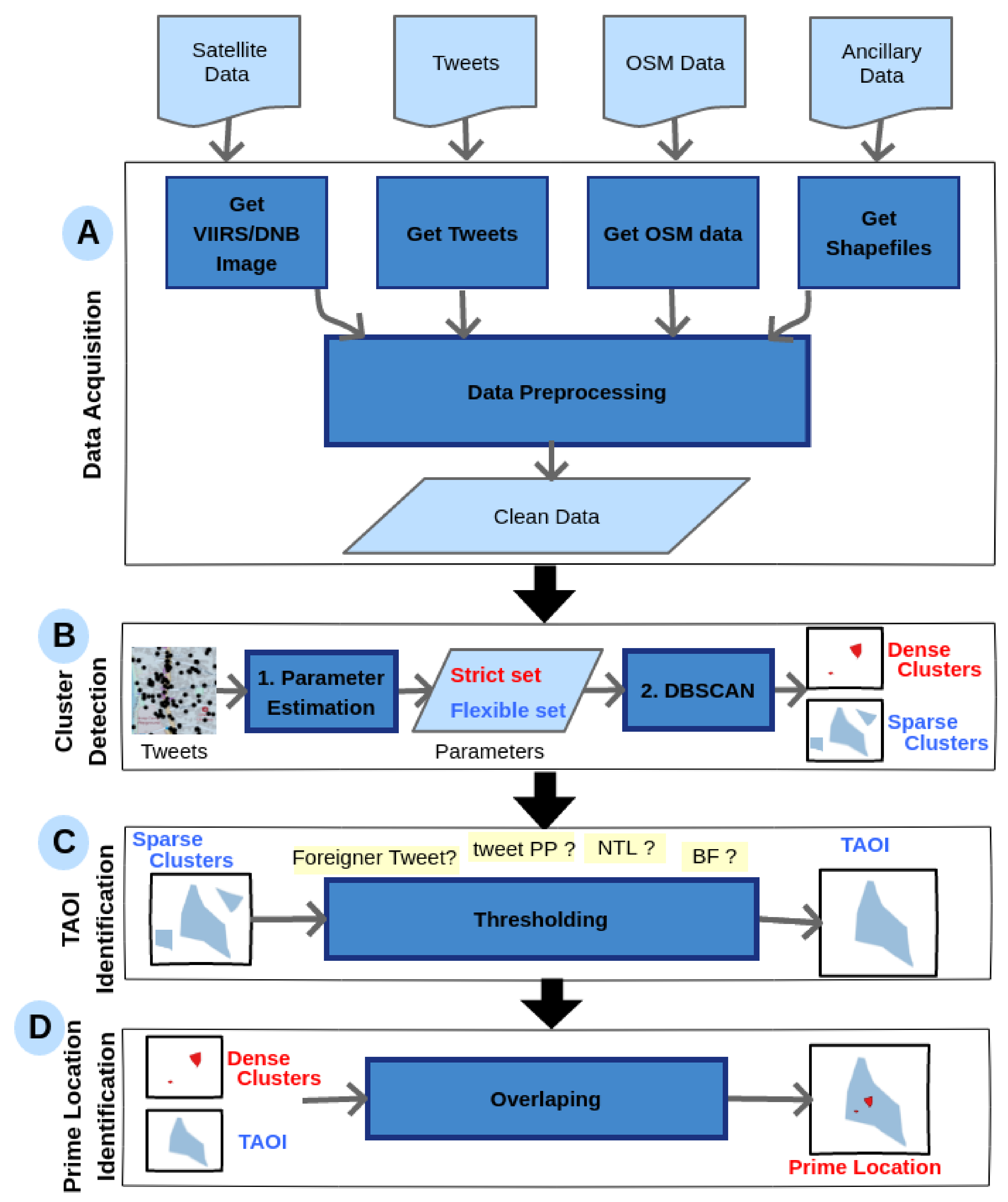
3. Methodology
3.1. Tourism Area of Interest (TAOI)
3.2. TAOI Identification Algorithm
- The algorithm should work in an unsupervised way as the exact number of clusters are not known beforehand.
- Clusters can have an arbitrary number, shape, or size (point percent) depending on the context (e.g., study area, data source, etc.)
- Method should detect high-intensity gathering of tweets all over the study area.
- The algorithm must aggregate significant data while discarding any outliers and noise.
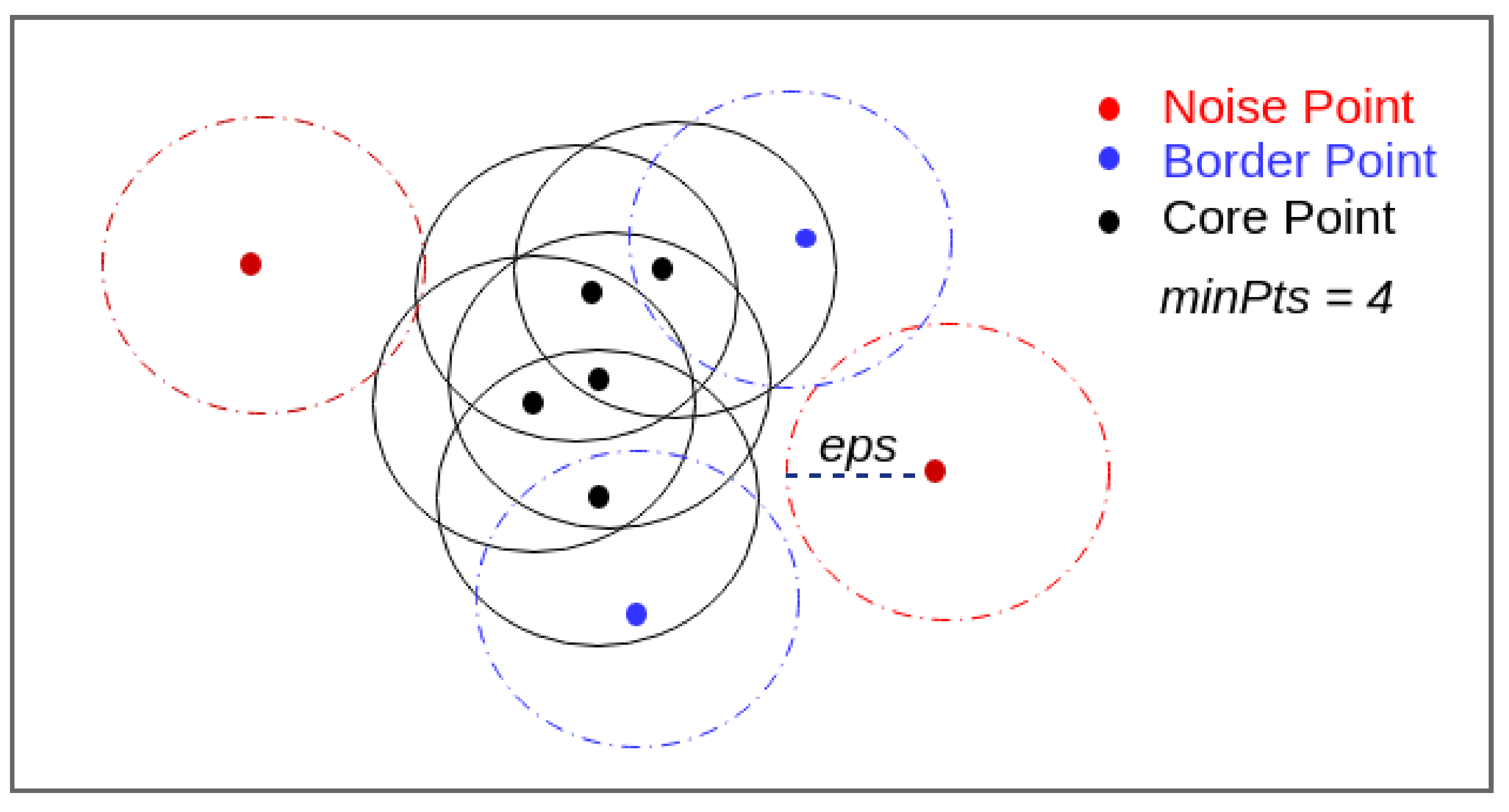
3.2.1. Clustering Terminology and Mechanism
- (i)
- The set of tweet points to be clustered is D, where p denotes the location of any tweet.
- (ii)
- The tweet density of a point p is determined by the number of neighboring tweets within distance from the point p.
- (iii)
- The -Neighborhood of p is represented by , where gives the distance between the two points p and q.
- (iv)
- A point p is a core point if it has a minimum of points within its neighborhood such that: .
- (v)
- A point q is a border point if it has fewer than points within its neighborhood but lies within the neighborhood of core point p.
- (vi)
- Any tweet point r which is neither a core nor a border point is considered to be a noise point.
- (vii)
- A point p is directly density reachable from another points q if p is within -Neighborhood of q and q is a core point such that:
- (a)
- .
- (b)
- .
- (viii)
- A point p is density reachable from another points q if there is a series of core points leading p to q such that: , where denote core points.
- (ix)
- A cluster C is a non-empty subset of D where each point is density reachable such that:
- (a)
- if and p is density reachable from q then .
- (b)
- so that both p and q are density reachable from r.
- (i)
- Start with an arbitrary point
- (a)
- Determine the neighborhood points adhering to and requirements.
- (1)
- Recursively apply step for all new neighboring points.
- (b)
- Density reachable and density connected points are used to create a new cluster. Any other points are marked as noise. If the noise point satisfies and for a different point in later iterations then it can still be a cluster point.
- (c)
- All points within the cluster are marked visited.
- (ii)
- Repeat step with new unvisited points until all the points are marked visited or noise.
3.2.2. Tuning of Clustering Parameter
- (i)
- (i.e., lowest and highest ): The strict version of parameters identifies groups with the smallest possible extent and utmost tweet density (i.e., Dense Clusters). The Dense Clusters are supposed to have the highest user attention and are the potential regions for prime tourism locations.
- (ii)
- (i.e., parameter combination yielding maximum clusters): A maximum number of clusters may be obtained with relaxed DBSCAN parameters and such accumulations (i.e., Sparse Clusters) are the candidate TAOI locations.
3.2.3. Cluster Detection
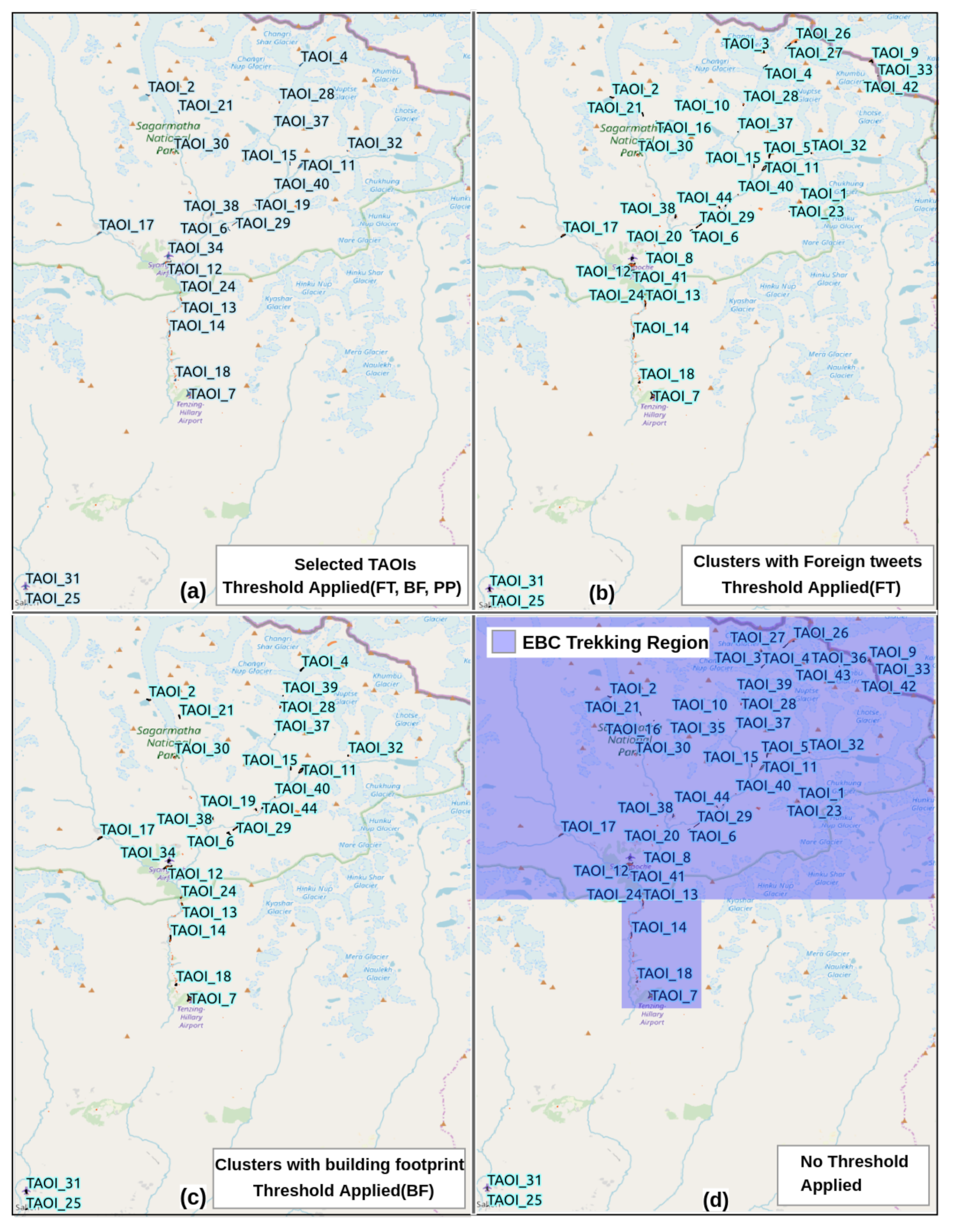
3.2.4. Identifying TAOIs by Cluster Pruning
- must be used to generate Sparse Clusters from geo-tagged tweets.
- Sparse Clusters must satisfy sufficient amount of foreigner tweets (FT) and tweet point percentage (PP).
- Lastly, BF and NTL thresholds must be fulfilled. Based on the contribution of BF and NTL, three different methods are defined to identify TAOIs as follows:
- (a)
- : Clusters must adhere to minimum BF threshold.
- (b)
- : Clusters must maintain minimum NTL threshold.
- (c)
- : Clusters must adhere to minimum NTL threshold as well as BF threshold.
- must be used to generate Dense Clusters from geo-tagged tweets.
- Dense Clusters must satisfy sufficient amounts of NTL, foreigner tweets, tweet point percentage, and building footprint requirements. Any cluster which does not meet these requirements are pruned away.
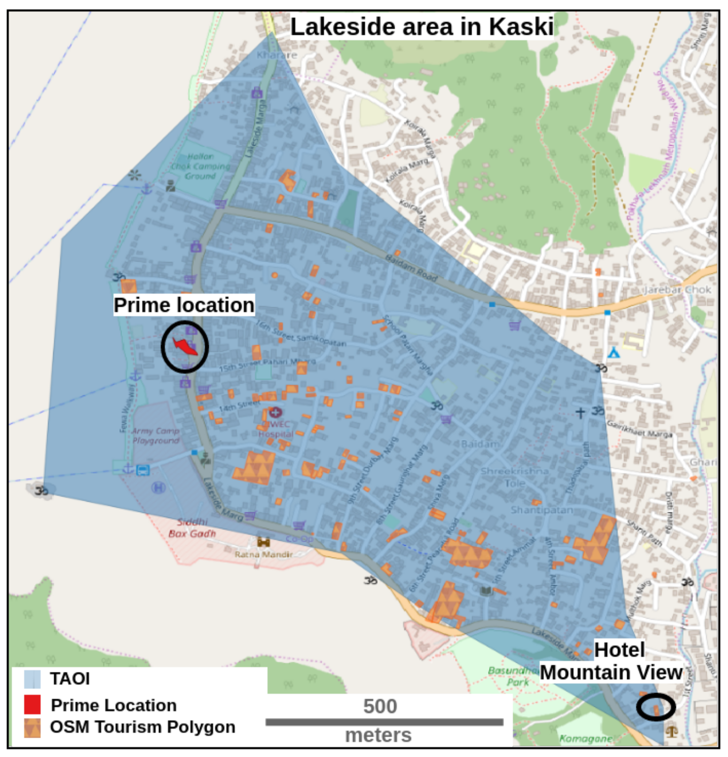
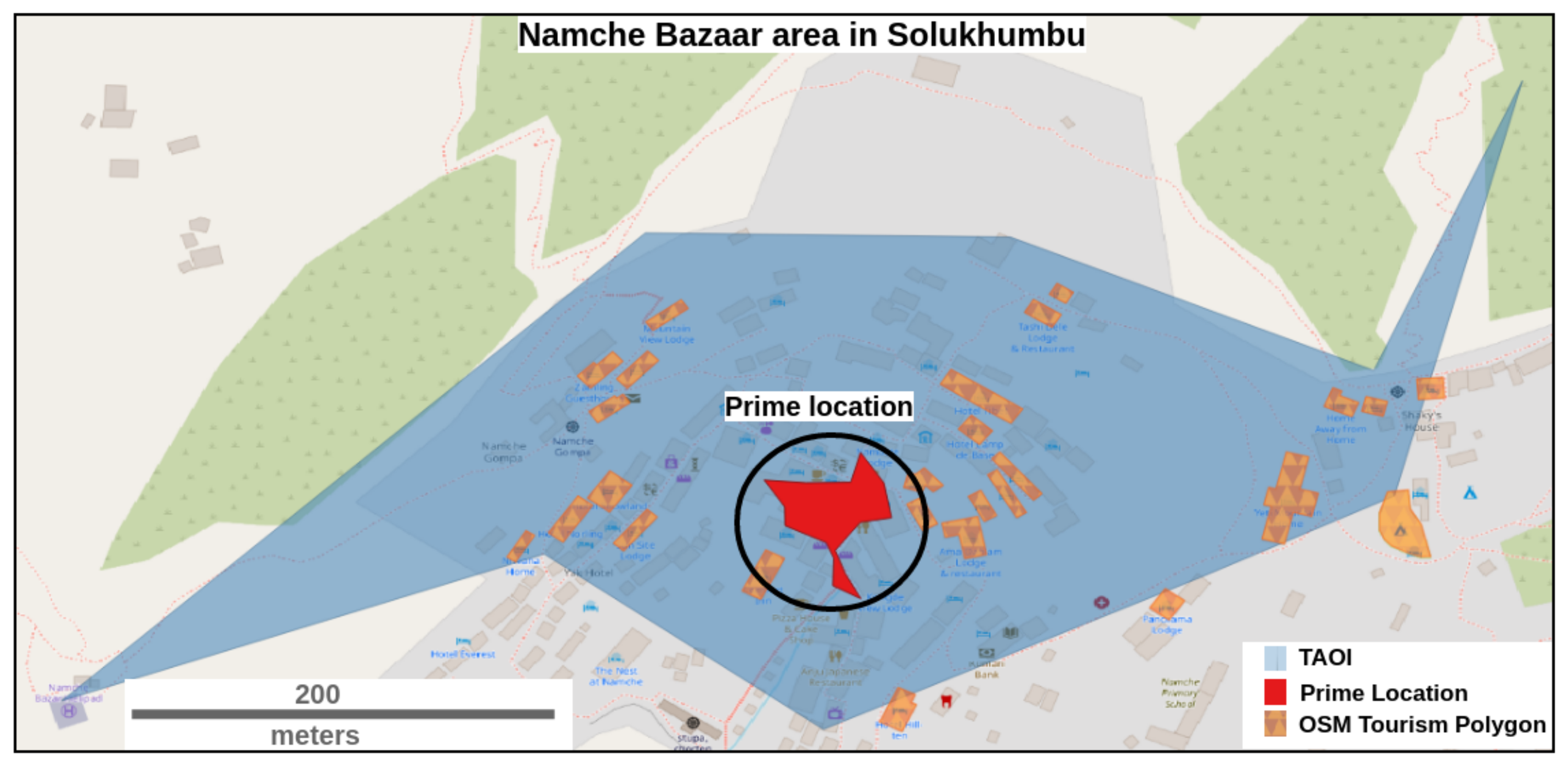
- The overlap of the selected Dense Clusters with TAOIs, if present, identifies the location of the prime tourism spots.
4. Experiment Setup
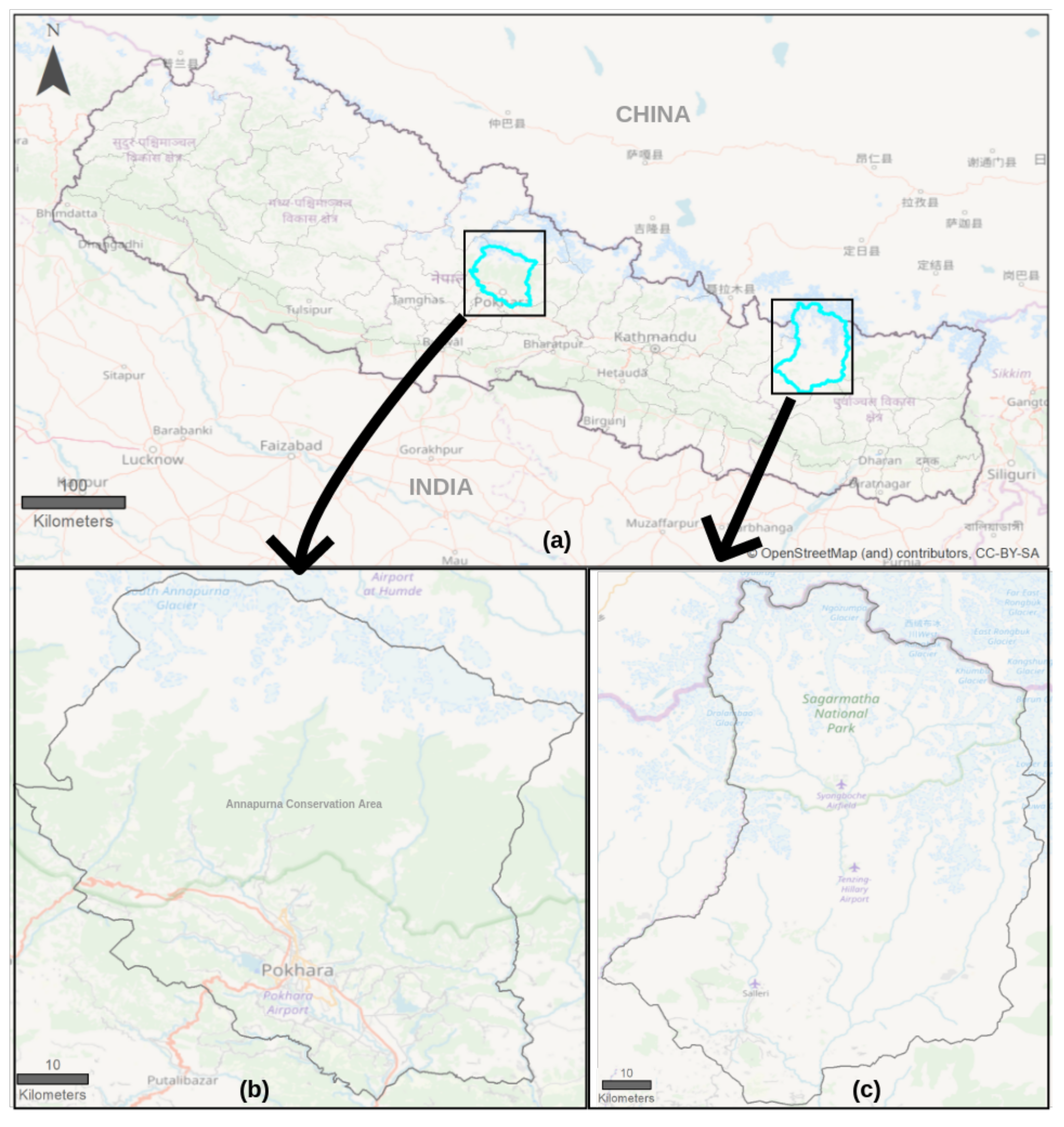
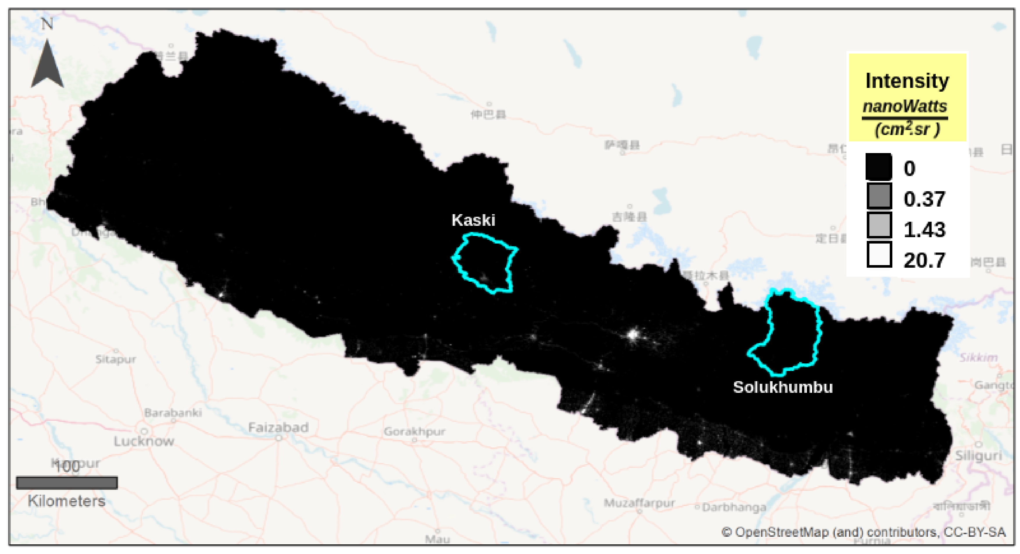
4.1. Study Area
4.2. Data Acquisition
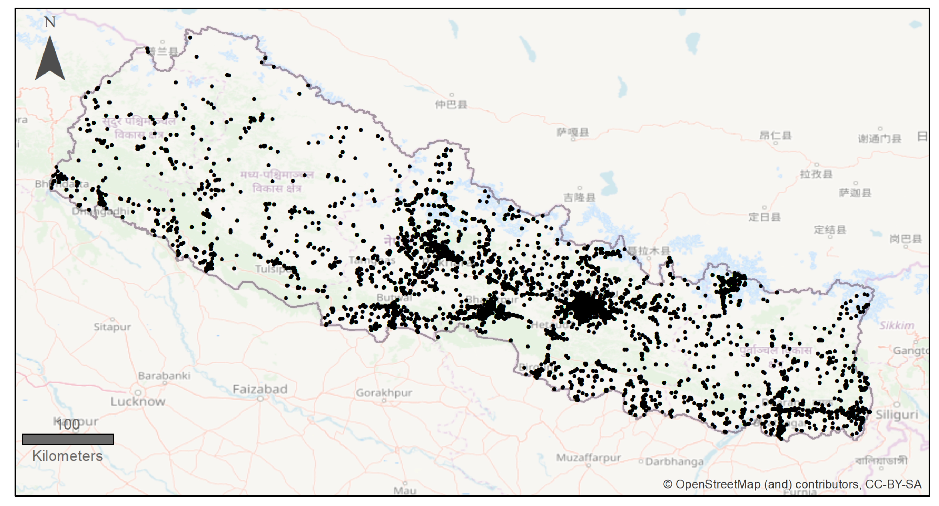
4.2.1. Twitter
4.2.2. Building Footprint
4.2.3. Nighttime Light
4.3. Softwares
5. Results
5.1. Selection of Clustering Parameters
5.2. TAOI Identification
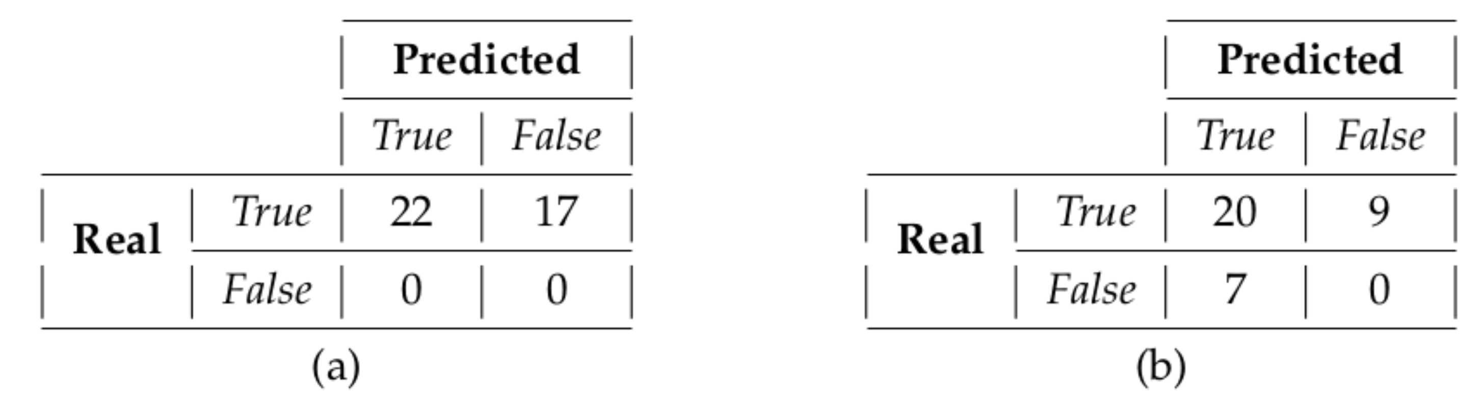
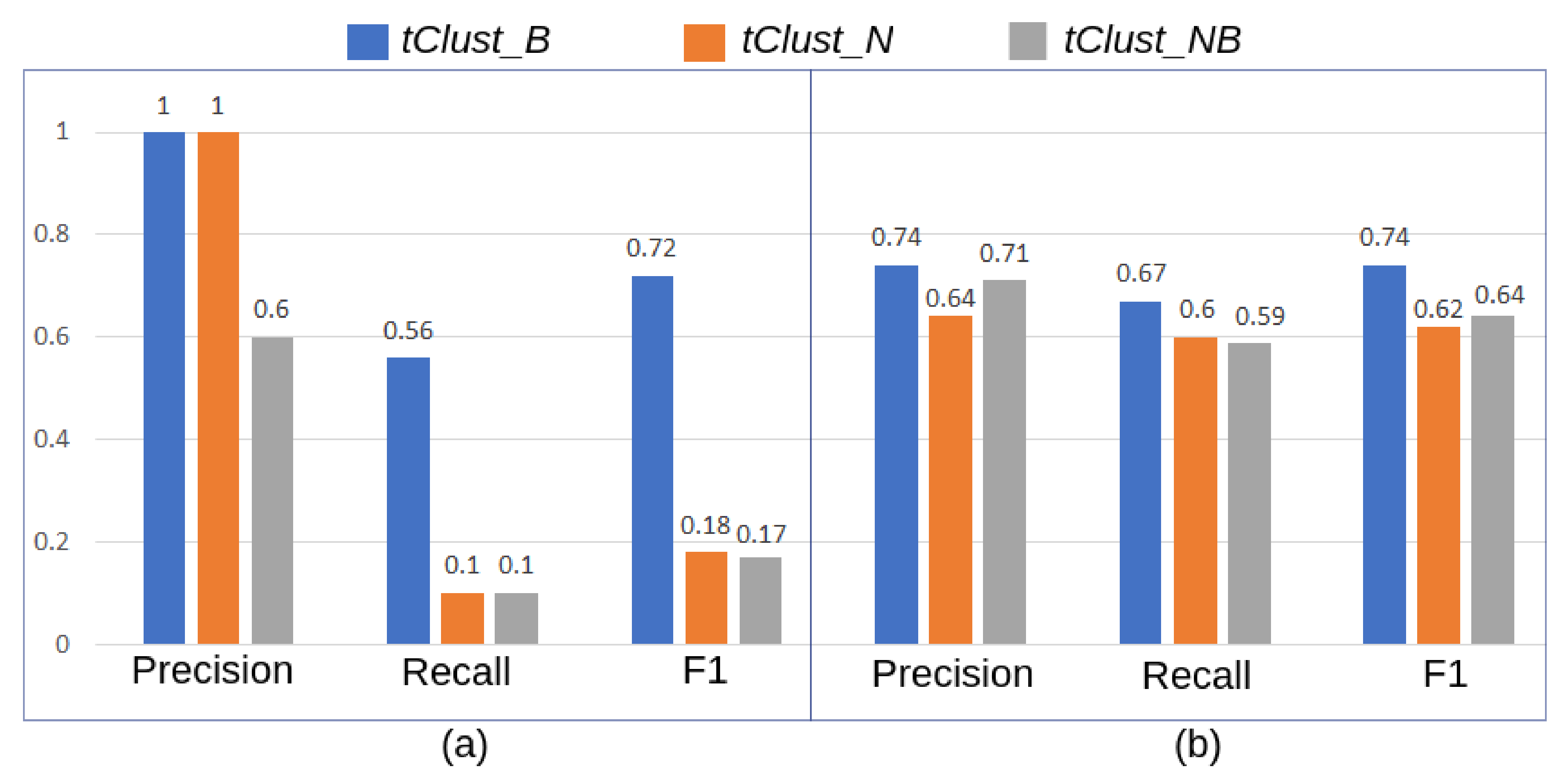
5.3. Validation
6. Discussion
6.1. Significance of the Data Sources Used
6.2. Significance of Cluster Pruning
6.3. TAOI Categorization
6.4. Cost Effective and Quicker Alternative to Traditional Methods
6.5. Comparison with OSM
6.6. Impact of Location Accuracy of Geo-Tagged Tweets
6.7. Limitations in Coverage
7. Conclusions
Author Contributions
Funding
Acknowledgments
Conflicts of Interest
References
- Ashley, C.; De Brine, P.; Lehr, A.; Wilde, H. The Role of the Tourism Sector in Expanding Economic Opportunity; John F. Kennedy School of Government, Harvard University Cambridge: Cambridge, MA, USA, 2007. [Google Scholar]
- WTTC. World Travel and Tourism Report 2018 Report for Nepal. Available online: https://www.wttc.org/-/media/files/reports/economic-impact-research/countries-2018/nepal2018.pdf (accessed on 18 March 2019).
- United Nations. Sustainable Tourism. Available online: https://sustainabledevelopment.un.org/topics/sustainabletourism (accessed on 27 June 2019).
- Morrison-Saunders, A.; Hughes, M.; Pope, J.; Douglas, A.; Wessels, J.A. Understanding visitor expectations for responsible tourism in an iconic national park: Differences between local and international visitors. J. Ecotourism 2019, 1–11. [Google Scholar] [CrossRef]
- Martín Martín, J.M.; Guaita Martínez, J.M.; Molina Moreno, V.; Sartal Rodríguez, A. An Analysis of the Tourist Mobility in the Island of Lanzarote: Car Rental Versus More Sustainable Transportation Alternatives. Sustainability 2019, 11, 739. [Google Scholar] [CrossRef]
- Henderson, J.V.; Storeygard, A.; Weil, D.N. Measuring economic growth from outer space. Am. Econ. Rev. 2012, 102, 994–1028. [Google Scholar] [CrossRef] [PubMed]
- Bennett, P.; Giles, L.; Halevy, A.; Han, J.; Hearst, M.; Leskovec, J. Channeling the deluge: Research challenges for big data and information systems. In Proceedings of the 22nd ACM International Conference on Information & Knowledge Management, San Francisco, CA, USA, 27 October–1 November 2013; pp. 2537–2538. [Google Scholar]
- Heikinheimo, V.; Minin, E.D.; Tenkanen, H.; Hausmann, A.; Erkkonen, J.; Toivonen, T. User-generated geographic information for visitor monitoring in a national park: A comparison of social media data and visitor survey. ISPRS Int. J. Geo-Inf. 2017, 6, 85. [Google Scholar] [CrossRef]
- Jendryke, M.; Balz, T.; McClure, S.C.; Liao, M. Putting people in the picture: Combining big location-based social media data and remote sensing imagery for enhanced contextual urban information in Shanghai. Comput. Environ. Urban Syst. 2017, 62, 99–112. [Google Scholar] [CrossRef] [Green Version]
- Miyazaki, H.; Nagai, M.; Shibasaki, R. Development of Time-Series Human Settlement Mapping System using Historical Landsat Archive. Int. Arch. Photogramm. Remote. Sens. Spat. Inf. Sci. 2016, 41, 1385. [Google Scholar] [CrossRef]
- Sitthi, A.; Nagai, M.; Dailey, M.; Ninsawat, S. Exploring land use and land cover of geotagged social-sensing images using naive bayes classifier. Sustainability 2016, 8, 921. [Google Scholar] [CrossRef]
- Preoţiuc-Pietro, D.; Volkova, S.; Lampos, V.; Bachrach, Y.; Aletras, N. Studying user income through language, behaviour and affect in social media. PLoS ONE 2015, 10, e0138717. [Google Scholar] [CrossRef] [PubMed]
- Levin, N.; Lechner, A.M.; Brown, G. An evaluation of crowdsourced information for assessing the visitation and perceived importance of protected areas. Appl. Geogr. 2017, 79, 115–126. [Google Scholar] [CrossRef] [Green Version]
- Park, J.H.; Lee, C.; Yoo, C.; Nam, Y. An analysis of the utilization of Facebook by local Korean governments for tourism development and the network of smart tourism ecosystem. Int. J. Inf. Manag. 2016, 36, 1320–1327. [Google Scholar] [CrossRef]
- Del Vecchio, P.; Mele, G.; Ndou, V.; Secundo, G. Creating value from social big data: Implications for smart tourism destinations. Inf. Process. Manag. 2018, 54, 847–860. [Google Scholar] [CrossRef]
- García-Palomares, J.C.; Gutiérrez, J.; Mínguez, C. Identification of tourist hot spots based on social networks: A comparative analysis of European metropolises using photo-sharing services and GIS. Appl. Geogr. 2015, 63, 408–417. [Google Scholar] [CrossRef]
- Encalada, L.; Boavida-Portugal, I.; Cardoso Ferreira, C.; Rocha, J. Identifying tourist places of interest based on digital imprints: Towards a sustainable smart city. Sustainability 2017, 9, 2317. [Google Scholar] [CrossRef]
- Maeda, T.; Yoshida, M.; Toriumi, F.; Ohashi, H. Extraction of Tourist Destinations and Comparative Analysis of Preferences Between Foreign Tourists and Domestic Tourists on the Basis of Geotagged Social Media Data. ISPRS Int. J. Geo-Inf. 2018, 7, 99. [Google Scholar] [CrossRef]
- Chen, M.; Arribas-Bel, D.; Singleton, A. Understanding the dynamics of urban areas of interest through volunteered geographic information. J. Geogr. Syst. 2018. [Google Scholar] [CrossRef]
- Majid, A.; Chen, L.; Mirza, H.T.; Hussain, I.; Chen, G. A system for mining interesting tourist locations and travel sequences from public geo-tagged photos. Data Knowl. Eng. 2015, 95, 66–86. [Google Scholar] [CrossRef]
- Vu, H.Q.; Li, G.; Law, R.; Ye, B.H. Exploring the travel behaviors of inbound tourists to Hong Kong using geotagged photos. Tour. Manag. 2015, 46, 222–232. [Google Scholar] [CrossRef]
- Lee, J.Y.; Tsou, M.H. Mapping Spatiotemporal Tourist Behaviors and Hotspots Through Location-Based Photo-Sharing Service (Flickr) Data. In Lecture Notes in Geoinformation and Cartography, Proceedings of the Progress in Location Based Services 2018, LBS 2018, Zurich, Switzerland, 15–17 January 2018; Kiefer, P., Huang, H., Van de Weghe, N., Raubal, M., Eds.; Springer International Publishing: Cham, Switzerland, 2018; pp. 315–334. [Google Scholar]
- Zhuang, C.; Ma, Q.; Liang, X.; Yoshikawa, M. Discovering obscure sightseeing spots by analysis of geo-tagged social images. In Proceedings of the 2015 IEEE/ACM International Conference on Advances in Social Networks Analysis and Mining 2015, Paris, France, 25–28 August 2015; pp. 590–595. [Google Scholar]
- Ester, M.; Kriegel, H.P.; Sander, J.; Xu, X. A density-based algorithm for discovering clusters in large spatial databases with noise. In Proceedings of the Second International Conference on Knowledge Discovery and Data Mining (KDD’96), Portland, OR, USA, 2–4 August 1996; Simoudis, E., Han, J., Fayyad, U., Eds.; AAAI Press: Palo Alto, CA, USA, 1996; Volume 96, pp. 226–231. [Google Scholar]
- Hu, Y.; Gao, S.; Janowicz, K.; Yu, B.; Li, W.; Prasad, S. Extracting and understanding urban areas of interest using geotagged photos. Comput. Environ. Urban Syst. 2015, 54, 240–254. [Google Scholar] [CrossRef]
- Liu, Y.; Liu, X.; Gao, S.; Gong, L.; Kang, C.; Zhi, Y.; Chi, G.; Shi, L. Social sensing: A new approach to understanding our socioeconomic environments. Ann. Assoc. Am. Geogr. 2015, 105, 512–530. [Google Scholar] [CrossRef]
- Goodchild, M.F. Citizens as sensors: The world of volunteered geography. GeoJournal 2007, 69, 211–221. [Google Scholar] [CrossRef]
- Haklay, M. How good is volunteered geographical information? A comparative study of OpenStreetMap and Ordnance Survey datasets. Environ. Plan. Plan. Des. 2010, 37, 682–703. [Google Scholar] [CrossRef]
- Li, L.; Goodchild, M.F. Constructing places from spatial footprints. In Proceedings of the 1st ACM SIGSPATIAL International Workshop on Crowdsourced and Volunteered Geographic Information, Redondo Beach, CA, USA, 6 November 2012; pp. 15–21. [Google Scholar]
- Salas-Olmedo, M.H.; Moya-Gómez, B.; García-Palomares, J.C.; Gutiérrez, J. Tourists’ digital footprint in cities: Comparing Big Data sources. Tour. Manag. 2018, 66, 13–25. [Google Scholar] [CrossRef]
- Estima, J.; Painho, M. Exploratory analysis of OpenStreetMap for land use classification. In Proceedings of the Second ACM SIGSPATIAL International Workshop on Crowdsourced and Volunteered Geographic Information, Orlando, FL, USA, 5 November 2013; pp. 39–46. [Google Scholar]
- Sun, Y.; Fan, H.; Li, M.; Zipf, A. Identifying the city center using human travel flows generated from location-based social networking data. Environ. Plan. Plan. Des. 2016, 43, 480–498. [Google Scholar] [CrossRef]
- Koutras, A.; Nikas, I.A.; Panagopoulos, A. Towards Developing Smart Cities: Evidence from GIS Analysis on Tourists’ Behavior Using Social Network Data in the City of Athens. In Smart Tourism as a Driver for Culture and Sustainability; Katsoni, V., Segarra-Oña, M., Eds.; Springer International Publishing: Cham, Switzerland, 2019; pp. 407–418. [Google Scholar]
- Xing, H.; Meng, Y.; Hou, D.; Song, J.; Xu, H. Employing crowdsourced geographic information to classify land cover with spatial clustering and topic model. Remote. Sens. 2017, 9, 602. [Google Scholar] [CrossRef]
- Li, Y.; Li, Q.; Shan, J. Discover patterns and mobility of Twitter users—A study of four US college cities. ISPRS Int. J. Geo-Inf. 2017, 6, 42. [Google Scholar] [CrossRef]
- Mazanec, J. Segmenting city tourists into vacation styles. In International City Tourism: Analysis and Strategy; Pinter: London, UK, 1997; pp. 114–128. [Google Scholar]
- Shoval, N.; Raveh, A. Categorization of tourist attractions and the modeling of tourist cities: Based on the co-plot method of multivariate analysis. Tour. Manag. 2004, 25, 741–750. [Google Scholar] [CrossRef]
- MacQueen, J. Some methods for classification and analysis of multivariate observations. In Proceedings of the Fifth Berkeley Symposium on Mathematical Statistics and Probability, Oakland, CA, USA, 21 June–18 July 1965; University of California Press: Berkeley, CA, USA, 1967; Volume 1, pp. 281–297. [Google Scholar]
- Rousseeuw, P.J.; Kaufman, L. Clustering by means of medoids. In Statistical Data Analysis Based on the L1 Norm and Related Methods; Dodge, Y., Ed.; North-Holland/Elsevier: Amsterdam, The Netherlands, 1987; pp. 405–416. [Google Scholar]
- Birant, D.; Kut, A. ST-DBSCAN: An algorithm for clustering spatial–temporal data. Data Knowl. Eng. 2007, 60, 208–221. [Google Scholar] [CrossRef]
- Kisilevich, S.; Mansmann, F.; Keim, D. P-DBSCAN: A density based clustering algorithm for exploration and analysis of attractive areas using collections of geo-tagged photos. In Proceedings of the 1st International Conference and Exhibition on Computing for Geospatial Research & Application, Washington, DC, USA, 21–23 June 2010; p. 38. [Google Scholar]
- Campello, R.J.; Moulavi, D.; Sander, J. Density-based clustering based on hierarchical density estimates. In Proceedings of the Pacific-Asia Conference on Knowledge Discovery and Data Mining, Gold Coast, Australia, 14–17 April 2013; Springer: Berlin/Heidelberg, Germany, 2013; pp. 160–172. [Google Scholar]
- Anselin, L. Local indicators of spatial association—LISA. Geogr. Anal. 1995, 27, 93–115. [Google Scholar] [CrossRef]
- Getis, A.; Ord, J. The Analysis of Spatial Association by Use of Distance Statistics, Geographycal Analysis. In Perspectives on Spatial Data Analysis; Springer: Berlin/Heidelberg, Germany, 1992. [Google Scholar]
- Wang, T.; Ren, C.; Luo, Y.; Tian, J. NS-DBSCAN: A Density-Based Clustering Algorithm in Network Space. ISPRS Int. J. Geo-Inf. 2019, 8, 218. [Google Scholar] [CrossRef]
- Dehuri, S.; Mohapatra, C.; Ghosh, A.; Mall, R. Comparative study of clustering algorithms. Inf. Technol. J. 2006, 5, 551–559. [Google Scholar] [CrossRef]
- Yang, Y.; Gong, Z. Identifying points of interest by self-tuning clustering. In Proceedings of the 34th International ACM SIGIR Conference on Research and Development in Information Retrieval, Beijing, China, 24–28 July 2011; pp. 883–892. [Google Scholar]
- Laptev, D.; Tikhonov, A.; Serdyukov, P.; Gusev, G. Parameter-free discovery and recommendation of areas-of-interest. In Proceedings of the 22nd ACM SIGSPATIAL International Conference on Advances in Geographic Information Systems, Dallas, TX, USA, 4–7 November 2014; pp. 113–122. [Google Scholar]
- Korakakis, M.; Spyrou, E.; Mylonas, P.; Perantonis, S.J. Exploiting social media information toward a context-aware recommendation system. Soc. Netw. Anal. Min. 2017, 7, 42. [Google Scholar] [CrossRef]
- Hasnat, M.M.; Hasan, S. Identifying tourists and analyzing spatial patterns of their destinations from location-based social media data. Transp. Res. Part Emerg. Technol. 2018, 96, 38–54. [Google Scholar] [CrossRef]
- Kuo, C.L.; Chan, T.C.; Fan, I.; Zipf, A. Efficient Method for POI/ROI Discovery Using Flickr Geotagged Photos. ISPRS Int. J. Geo-Inf. 2018, 7, 121. [Google Scholar] [CrossRef]
- Yan, Y.; Kuo, C.L.; Feng, C.C.; Huang, W.; Fan, H.; Zipf, A. Coupling maximum entropy modeling with geotagged social media data to determine the geographic distribution of tourists. Int. J. Geogr. Inf. Sci. 2018, 32, 1699–1736. [Google Scholar] [CrossRef]
- Cheng, Y. Mean shift, mode seeking, and clustering. IEEE Trans. Pattern Anal. Mach. Intell. 1995, 17, 790–799. [Google Scholar] [CrossRef]
- Rosenblatt, M. Remarks on some nonparametric estimates of a density function. In The Annals of Mathematical Statistics; JSTOR: New York, NY, USA, 1956; pp. 832–837. [Google Scholar]
- Dueck, D. Affinity Propagation: Clustering Data by Passing Messages. Ph.D. Thesis, University of Toronto, Toronto, ON, Canada, 2009. [Google Scholar]
- Ng, A.Y.; Jordan, M.I.; Weiss, Y. On spectral clustering: Analysis and an algorithm. In Advances in Neural Information Processing Systems; MIT Press: Cambridge, MA, USA, 2001; pp. 849–856. [Google Scholar]
- Schubert, E.; Sander, J.; Ester, M.; Kriegel, H.P.; Xu, X. DBSCAN revisited, revisited: Why and how you should (still) use DBSCAN. ACM Trans. Database Syst. (TODS) 2017, 42, 19. [Google Scholar] [CrossRef]
- Zhou, X.; Xu, C.; Kimmons, B. Detecting tourism destinations using scalable geospatial analysis based on cloud computing platform. Comput. Environ. Urban Syst. 2015, 54, 144–153. [Google Scholar] [CrossRef]
- Akdag, F.; Eick, C.F.; Chen, G. Creating Polygon Models for Spatial Clusters. In Foundations of Intelligent Systems; Andreasen, T., Christiansen, H., Cubero, J.C., Raś, Z.W., Eds.; Springer International Publishing: Cham, Switzerland, 2014; pp. 493–499. [Google Scholar] [Green Version]
- Duckham, M.; Kulik, L.; Worboys, M.; Galton, A. Efficient generation of simple polygons for characterizing the shape of a set of points in the plane. Pattern Recognit. 2008, 41, 3224–3236. [Google Scholar] [CrossRef]
- Devkota, B.; Miyazaki, H. An Exploratory Study on the Generation and Distribution of Geotagged Tweets in Nepal. In Proceedings of the 2018 IEEE 3rd International Conference on Computing, Communication and Security (ICCCS), Kathmandu, Nepal, 25–27 October 2018; pp. 70–76. [Google Scholar]
- Yamaguchi, Y.; Amagasa, T.; Kitagawa, H. Landmark-based user location inference in social media. In Proceedings of the First ACM Conference on Online Social Networks, Boston, MA, USA, 7–8 October 2013; pp. 223–234. [Google Scholar]
- Chong, W.H.; Lim, E.P. Fine-grained Geolocation of Tweets in Temporal Proximity. ACM Trans. Inf. Syst. (TOIS) 2019, 37, 17. [Google Scholar] [CrossRef]
- Jurgens, D. That’s what friends are for: Inferring location in online social media platforms based on social relationships. In Proceedings of the Seventh International AAAI Conference on Weblogs and Social Media, Atlanta, GA, USA, 28 June 2013. [Google Scholar]
- Krikigianni, E.; Tsiakos, C.; Chalkias, C. Estimating the relationship between touristic activities and night light emissions. Eur. J. Remote. Sens. 2019, 52, 233–246. [Google Scholar] [CrossRef] [Green Version]
- Checa, J. Urban Intensities. The Urbanization of the Iberian Mediterranean Coast in the Light of Nighttime Satellite Images of the Earth. Urban Sci. 2018, 2, 115. [Google Scholar] [CrossRef]
- Nepal, S.K.; Kohler, T.; Banzhaf, B.R. Great Himalaya: Tourism and the Dynamics of Change in Nepal; Swiss Foundation for Alpine Research: Zurich, Switzerland, 2002. [Google Scholar]
- Central Bureau of Statistics, Government of Nepal. National Population and Housing Census 2011. Available online: https://unstats.un.org/unsd/demographic/sources/census/wphc/Nepal/Nepal-Census-2011-Vol1.pdf (accessed on 18 March 2019).
- LonelyPlanet. Top Experiences in Nepal. Available online: https://www.lonelyplanet.com/nepal (accessed on 7 April 2019).
- InternetLiveStats. Twitter Usage Statistics. 2013. Available online: http://www.internetlivestats.com/twitter-statistics/ (accessed on 18 March 2019).
- Cesare, N.; Grant, C.; Nsoesie, E.O. Detection of User Demographics on Social Media: A Review of Methods and Recommendations for Best Practices. arXiv 2017, arXiv:1702.01807. [Google Scholar]
- Burghardt, M. Tools for the Analysis and Visualization of Twitter Language Data. Available online: https://epub.uni-regensburg.de/35669/ (accessed on 18 March 2019).
- Puschmann, C.; Bruns, A.; Mahrt, M.; Weller, K.; Burgess, J. Epilogue: Why Study Twitter. In Twitter and Society; Peter Lang: New York, NY, USA, 2014; Volume 89, pp. 425–432. [Google Scholar]
- SocialAves. Social Media Landscape Nepal. 2017. Available online: https://socialaves.com/social-media-landscape-nepal/ (accessed on 18 March 2019).
- Li, L.; Goodchild, M.F.; Xu, B. Spatial, temporal, and socioeconomic patterns in the use of Twitter and Flickr. Cartogr. Geogr. Inf. Sci. 2013, 40, 61–77. [Google Scholar] [CrossRef]
- Morstatter, F.; Pfeffer, J.; Liu, H.; Carley, K.M. Is the sample good enough? comparing data from twitter’s streaming api with twitter’s firehose. arXiv 2013, arXiv:1306.5204. [Google Scholar]
- Morstatter, F.; Pfeffer, J.; Liu, H. When is it biased? Assessing the representativeness of twitter’s streaming API. In Proceedings of the 23rd International Conference on World Wide Web, Seoul, Korea, 7–11 April 2014; pp. 555–556. [Google Scholar]
- Frias-Martinez, V.; Soto, V.; Hohwald, H.; Frias-Martinez, E. Characterizing urban landscapes using geolocated tweets. In Proceedings of the 2012 International Conference on Privacy, Security, Risk and Trust and 2012 International Confernece on Social Computing, Amsterdam, The Netherlands, 3–5 September 2012; pp. 239–248. [Google Scholar]
- Zhao, N.; Cao, G.; Zhang, W.; Samson, E.L. Tweets or nighttime lights: Comparison for preeminence in estimating socioeconomic factors. ISPRS J. Photogramm. Remote. Sens. 2018, 146, 1–10. [Google Scholar] [CrossRef]
- Elvidge, C.D.; Safran, J.; Tuttle, B.; Sutton, P.; Cinzano, P.; Pettit, D.; Arvesen, J.; Small, C. Potential for global mapping of development via a nightsat mission. GeoJournal 2007, 69, 45–53. [Google Scholar] [CrossRef]
- Baugh, K.; Hsu, F.C.; Elvidge, C.D.; Zhizhin, M. Nighttime lights compositing using the VIIRS day-night band: Preliminary results. Proc. Asia-Pac. Adv. Netw. 2013, 35, 70–86. [Google Scholar] [CrossRef]
- Li, X.; Elvidge, C.; Zhou, Y.; Cao, C.; Warner, T. Remote sensing of night-time light. Int. J. Remote. Sens. 2017, 38, 5855–5859. [Google Scholar] [CrossRef] [Green Version]
- Mellander, C.; Lobo, J.; Stolarick, K.; Matheson, Z. Night-time light data: A good proxy measure for economic activity? PLoS ONE 2015, 10, e0139779. [Google Scholar] [CrossRef]
- Board, N.T. Greater Pokhara Valley Lake side and City Map. In Greater Pokhara Valley and City Map; Nepal Map Publisher: Kathmandu, Nepal, 2011. [Google Scholar]
- Banerjee, P.S. Everest Trekking Maps and Complete Guide; Milestone Himalayan Series; Milestone Books: Calcutta, India, 2017. [Google Scholar]
- Nel, O.; López, J.; Martín, J.; Checa, J. Energy and urban form. The growth of European cities on the basis of night-time brightness. Land Use Policy 2017, 61, 103–112. [Google Scholar] [CrossRef]
- Buntain, C.; McGrath, E.; Golbeck, J.; LaFree, G. Comparing Social Media and Traditional Surveys around the Boston Marathon Bombing. In Proceedings of the #Microposts: 6th Workshop on Making Sense of Microposts, Montréal, QC, Canada, 11–15 April 2016; pp. 34–41. [Google Scholar]
- Zheng, S.; Zheng, J. Assessing the completeness and positional accuracy of OpenStreetMap in China. In Thematic Cartography for the Society; Springer: Cham, Switzerland, 2014; pp. 171–189. [Google Scholar]
- Tomaštík, J.; Saloň, Š.; Piroh, R. Horizontal accuracy and applicability of smartphone GNSS positioning in forests. For. Int. J. For. Res. 2016, 90, 187–198. [Google Scholar] [CrossRef]
- Merry, K.; Bettinger, P. Smartphone GPS accuracy study in an urban environment. PLoS ONE 2019, 14, e0219890. [Google Scholar] [CrossRef] [PubMed]


| Algorithm | Comments |
|---|---|
| DBSCAN [24] | - Works in an unsupervised way as the exact number of clusters are not known beforehand. - Clusters can have an arbitrary number, shape, or size. - Detects high-intensity gathering of points all over the study area. - Aggregates significant data while discarding any outliers and noise. - Require minimum domain knowledge to determine the input parameters. |
| Classic clustering method such as K-means [38] and K-medoids [39] | - Require pre-knowledge of the number of clusters to be generated. - Cannot identify outliers as noise. - Final result is sensitive to initial starting values. - Assumes the true underlying clusters are globular. |
| Spatial Point Processing methods such as Local Moran [43] and Getic-ord Gi [44] | - Cannot outperform generic clustering algorithms ( e.g., DBSCAN) in delineating aggregated data and shaping generated clusters. |
| Self-Organizing Maps [46] | - If the clusters are of arbitrary shape, DBSCAN algorithm performs better than the self-organizing map. |
| Mean-Shift Algorithm [53] | - Cannot identify outliers as noise. |
| Kernel Density Estimation [54] | - Does not generate a clear hard-lined definitions between points in different clusters. |
| Affinity Propagation [55] | - Assumes the true underlying clusters are globular. |
| Spectral clustering [56] | - Require pre-knowledge of the number of clusters to be generated. |
| Kaski | Solukhumbu | |
|---|---|---|
| Area ( sq.km.) | 2017 | 3312 |
| Population | 492,098 | 105,886 |
| Bounding Box(degrees) | (83.70,28.08), (84.28,28.61) | (86.36,27.34), (87.01,28.11) |
| Features | - Pokhara, the tourism capital of Nepal. - Pokhara ranked 7 in “Top Experiences in Nepal” by Lonely Planet [69]. - A part of Mount Annapurna and range. | - Mount Everest. - World heritage site: Sagarmatha National Park. - ‘Everest Base Camp Trek’ ranked 2 in “Top Experiences in Nepal” by Lonely Planet [69]. |
| Place | Total Tweets | Total Users | Average Tweets Per User |
|---|---|---|---|
| Kaski | 8787 | 2150 | 4 |
| Solukhumbu | 5472 | 718 | 7 |
| Nepal | 89,228 | 14,216 | 6 |
| NTL 2015 | NTL 2016 | |
|---|---|---|
| NTL 2015 | 1 | 0.995 |
| NTL 2016 | 0.995 | 1 |
| Place | ||||||
|---|---|---|---|---|---|---|
| (m) | (%) | Clusters | (m) | (%) | Clusters | |
| Kaski | 25 | 0.11 | 1 | 175 | 0.01 | 75 |
| Solukhumbu | 25 | 0.51 | 1 | 350 | 0.01 | 44 |
| Place | Total Clusters | Clusters Confirming | |||
|---|---|---|---|---|---|
| FT | NTL | BF | PP | ||
| Kaski | 75 | 47 | 60 | 68 | 68 |
| Solukhumbu | 44 | 39 | 7 | 26 | 40 |
| Place | Total Clusters | tClust_B | tClust_N | tClust_NB | Prime Location | |||
|---|---|---|---|---|---|---|---|---|
| TAOI | Pruned | TAOI | Pruned | TAOI | Pruned | |||
| Kaski | 75 | 41 | 34 | 33 | 42 | 28 | 47 | 1 |
| Solukhumbu | 44 | 24 | 20 | 7 | 37 | 5 | 39 | 1 |
| Place | tClust_B | Prime Locations | ||
|---|---|---|---|---|
| TAOIs | Overlap | Locations | Overlap | |
| Kaski | 41 | 19 | 1 | 0 |
| Solukhumbu | 24 | 13 | 1 | 0 |
© 2019 by the authors. Licensee MDPI, Basel, Switzerland. This article is an open access article distributed under the terms and conditions of the Creative Commons Attribution (CC BY) license (http://creativecommons.org/licenses/by/4.0/).
Share and Cite
Devkota, B.; Miyazaki, H.; Witayangkurn, A.; Kim, S.M. Using Volunteered Geographic Information and Nighttime Light Remote Sensing Data to Identify Tourism Areas of Interest. Sustainability 2019, 11, 4718. https://0-doi-org.brum.beds.ac.uk/10.3390/su11174718
Devkota B, Miyazaki H, Witayangkurn A, Kim SM. Using Volunteered Geographic Information and Nighttime Light Remote Sensing Data to Identify Tourism Areas of Interest. Sustainability. 2019; 11(17):4718. https://0-doi-org.brum.beds.ac.uk/10.3390/su11174718
Chicago/Turabian StyleDevkota, Bidur, Hiroyuki Miyazaki, Apichon Witayangkurn, and Sohee Minsun Kim. 2019. "Using Volunteered Geographic Information and Nighttime Light Remote Sensing Data to Identify Tourism Areas of Interest" Sustainability 11, no. 17: 4718. https://0-doi-org.brum.beds.ac.uk/10.3390/su11174718