Experimental and Numerical Study on the Characteristics of the Thermal Design of a Large-Area Hot Plate for Nanoimprint Equipment


1
HSD Engine Ltd., Changwon-ci, Kyungsangnam-do, Changwon 51574, Korea
2
Department of Mechanical and Shipbuilding Convergence Engineering, Pukyung National University, Busan 48547, Korea
*
Author to whom correspondence should be addressed.
Sustainability 2019, 11(17), 4795; https://0-doi-org.brum.beds.ac.uk/10.3390/su11174795
Submission received: 15 August 2019
/
Revised: 28 August 2019
/
Accepted: 29 August 2019
/
Published: 3 September 2019
Abstract
:A numerical study was conducted on the thermal performance of a large-area hot plate specifically designed as a heating and cooling tool for thermal nanoimprint lithography processes. The hot plate had the dimensions 240 mm × 240 mm × 20 mm, in which a series of cartridge heaters and cooling holes were installed. Stainless steel was selected to endure the high molding pressures. To examine the hot plate’s abnormal thermal behavior, ANSYS Fluent V15.0, which is commercial CFD code, was used to perform computational analysis. A numerical model was employed to predict the thermal behavior of the hot plate in both the heating and cooling phases. To conduct the thermal design of a large-area hot plate for nanoimprint equipment, we selected the model to be studied and proposed a cooling model using both direct and indirect cooling methods with and without heat pipes. In addition, we created a small hot plate and performed experimental and computational analyses to confirm the validity of the proposed model. This study also analyzed problems that may occur in the stage prior to the large-area expansion of the hot plate. In the case of a stainless steel (STS304) hot plate for large-area hot plate expansion, the heat pipes were inserted in the direction of the cartridge heaters to address the problems that may occur when expanding the hot plate into a large area. As a result, the heating rate was 40 °C/min and the temperature uniformity was less than 1% of the maximum working temperature of 200 °C. For cooling, when considering pressure and using air as the coolant for the ends, a cooling rate of 20 °C/min and thermal performance of less than 13.2 °C (less than 7%) based on the maximum temperature were obtained. These results were similar to the experimental results.
1. Introduction
A hot plate is a heating device that indirectly applies heat to a material via surface heating. It is widely used, with applications including cooking plates, temperature control devices for chemical experiments in which temperature uniformity is important, and semiconductor processing devices that require rapid uniform heating performance. General hot plate design is not difficult in view of the current level of industrial technology, and a variety of products are already available on the market. However, these have not been thoroughly researched. The subject of this study is a hot plate for thermal nanoimprint lithography (TH-NIL) equipment. The design of this type of hot plate is technically challenging due to the functional requirements demanded by the TH-NIL process. Mass production technology for creating various nano shapes is key to improving the performance and functionality of electronic components, as well as to improving manufacturing productivity. Photolithography has, to date, led the miniaturization of shapes in semiconductor processes [1]. This fabrication method uses the properties of photoreactive resin. It has been developed to the level of fabrication at 10-nm line width in memory semiconductor processes; however, due to the complexity of the fabrication process and high production costs, it is difficult to fabricate a diversity of shapes. Furthermore, due to the limitations of the wavelength of light, progress in miniaturization has also been stunted. An alternative to address these issues is the nanoimprint technique, a mechanical etching technique in which the polymer substrate is heated to a temperature above the glass transition temperature, softened, and then pressed against the surface using a stamp with an ultra-fine shape that transfers its opposite shape [2]. Based on resin solidification methods, this fabrication method is classified as a photo-curing method in which ultraviolet rays are irradiated onto a UV-curable resin, and as a TH-NIL method in which the resin is cured via cooling. As TH-NIL is not restricted by the ultraviolet wavelength of the photo-curing method, a fabrication method capable of producing high-aspect-ratio structures [3] or precise thermal control due to the continuous process of heating– pressurizing–cooling is required.
However, because the manufacturing process is complex, the cost of production is high and it is difficult to manufacture a variety of shapes. In addition, progress in miniaturization is encountering limitations due to constraints caused by light wavelengths [4,5,6]. One alternative which has been proposed for resolving this problem is nano imprinting. This is a mechanical etching method in which a polymer substrate is softened by heating it to higher than the glass transition temperature [7,8,9,10,11,12,13,14] and then a stamp with a nano-shape is pressed on the surface to transfer the opposite shape [15,16,17]. This manufacturing method is classified according to the method by which the resin is hardened, and it includes the photocuring method which uses ultraviolet radiation on the resin and the TH-NIL method which cools the resin to harden it. TH-NIL is not subject to the limitations caused by the photocuring method’s ultraviolet ray wavelengths, and it can create high aspect ratio shapes [18], but it requires fine thermal control due to the characteristics of the continuous heating– pressurizing– cooling process.
Even in the earliest publications from Chou et al. [2,19,20] this simple concept showed high-resolution capabilities down to the 10-nm regime. Various NIL methods are differentiated depending on the curing process applied, which also sets the required specifications for mold and resist materials. NIL methods with the corresponding materials used are summarized in Table 1.
The following requirements should be considered when designing the TH-NIL hot plate: (1) the hot plate should be able to rapidly heat and cool to efficiently melt and solidify the resin; (2) the hot plate should have large-area expandability; (3) the hot plate should maintain high temperature uniformity to minimize deformation due to non-uniform thermal expansion and to facilitate stamping and separation; (4) the hot plate material should have high hardness and strength to minimize deformation due to pressure during pressing. (1) and (2) are productivity-related requirements and (3) and (4) are quality-related requirements. Fully-fledged research on TH-NIL began after the proposal of Chou et al. [2]; however, these studies mostly cover physical phenomena such as filling that occur in processes, the material properties of substrates and the like, and stamp fabrication [25,26,27,28]. In contrast, researchers also conducted studies on hot plates in line with the promotion of TH-NIL equipment development [29,30,31]. Kwak et al. [32] proposed a concept for a hot plate capable of horizontal expansion of the cold source and heat source in which long rod-shaped cartridge heaters and cooling holes through which the coolant flows are vertically staggered They then verified its conceptual validity through computational analysis and experimentation. In a subsequent study, Park et al. [33] embodied the conceptual model presented in the previous study and designed a 240 × 240 × 20 mm hot plate, analyzed its thermal behavior through computational analysis, and found that the hot plate provides consistent heating performance and temperature uniformity satisfying the design requirements. In particular, this study created and utilized a sub-program capable of simulating proportional–integral–derivative (PID) control to reproduce the thermal behavior of a hot plate equipped with an actual feedback controller. This study used aluminum with high thermal diffusivity for the material of the hot plate to ensure temperature uniformity; however, aluminum has a low surface hardness, making it an unsuitable material for the TH-NIL process that is exposed to high pressure pressing. To address this problem, Yang [34] conducted a heating test using a hot plate fabricated from stainless steel with a high surface hardness. However, as a cooling test using the coolant flow in the cooling holes was not performed, the thermal performance of the entire process could not be evaluated.
This study aimed to evaluate the suitability of thermal design of a hot plate fabricated from stainless steel with a high material strength and hardness to withstand the pressurization process. For this purpose, we numerically analyzed the unsteady thermal behavior of the heating and cooling processes. In this process, this study identified thermal problems caused by stainless steel materials with low thermal conductivity and sought corresponding solutions.
2. Experimental and Analysis Method
2.1. Experimental Setup and Method
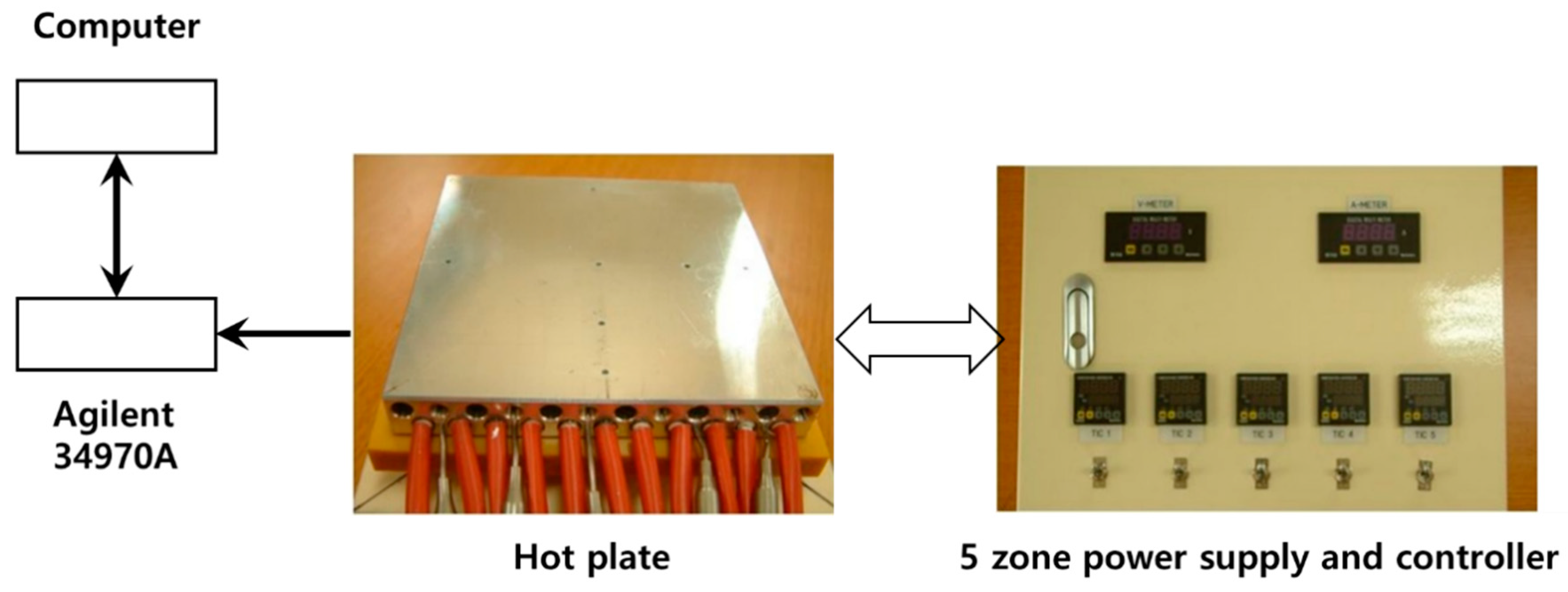
Figure 1 shows a schematic diagram of the experimental setup. The experimental setup consists of a power supply, a controller, and a temperature measurement device. The power supply and controller were integrated into a single system. When power is applied by the power supply, the temperature read by the thermocouple located at the center of the hot plate is inputted to the controller and compared with the target temperature, after which multiple control is performed. The target temperature was set to 240 °C.
Figure 2 shows the configuration of the controller, DC power relay, and heater which show the specification of instrument as shown Table 2. For the PID controller, the temperature of the hot plate is inputted into the feedback controller (TZN4S) through the thermocouple located at the center of the hot plate. The DC power supply relay (WYG 1C 20Z4), which interrupts the supply of current, is controlled to adjust the temperature of the heater in comparison with the target temperature. The thermocouple can be used at temperatures even above 1000 °C. We calibrated the K-type thermocouple with a diameter of 2.0 mm using a thermostat and observed a measurement error of 1.5 °C. The measurement position for temperature control is in the direction in which the cartridge heater is inserted as in the computer analysis, located at the center of the hot plate and 12 mm from the upper hot plate. To minimize heat loss from the lower part, the hot plate was placed on a peak heat insulation material with a thickness of 20 mm and connected to the temperature measurement device Agilent 34970A, that can measure 120 channels simultaneously and has a 22-bit resolution.
In the heating test, the temperature of the atmosphere in the laboratory was kept constant at 17 °C to keep the outside air temperature constant. The temperature sensor was operated in a constant state. Power was supplied to the hot plate after two minutes from the start of operation of the temperature sensor, as it takes some time to determine if the researcher has made a mistake, or if the internal settings of Agilent 34970A are operational. The target temperature was set to 240 degrees and the power was turned off 200 to 205 min after being supplied to the hot plate. The computational analysis was performed in the same manner, the details of which are covered in the numerical analysis method.
2.2. Numerical Method and Analytical Model
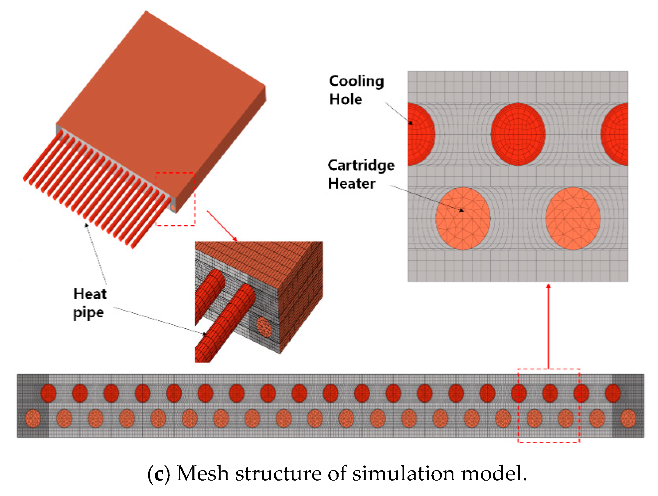
To examine the hot plate’s abnormal thermal behavior, ANSYS Fluent V15.0, which is commercial CFD (Computation Fluid Dynamics) code, was used to perform computational analysis. The analysis area was the entire hot plate as shown in Figure 1 and two million grid cells were used.
The RNG k-ε model [35] is a method of modeling the turbulence phenomenon based on a mathematical statistical technique called RNG (Renormalization Group) method. The transportation equation for k, ε of RNG model is as follows;
The coefficient values applied in the above equation are as follows;
where, is turbulent kinetic energy Prandtl number, is turbulent dissipation rate Prandtl number, is turbulent viscosity with , is turbulent energy dissipation rate, is strain tensor, is turbulent kinetic energy.
We developed a dedicated computational analysis model to analyze the thermal behavior of the hot plate. The physical mechanisms related to the thermal behavior of the hot plate include the heat generation of the cartridge heaters used as the heating source and the convection heat transfer of the coolant in the cooling holes, or the cooling at the ends of the heat pipes and the natural convection heat transfer from the surface of the hot plate to the outside air. Because of high computational and physical complexity, numerical simulation of all these heating mechanisms is not suitable for use as a thermal design tool. This study treated the heat transfer from the hot plate to the outside air as a boundary condition to fulfill the objectives of the thermal design of the hot plate. For the computational analysis, we used ANSYS Fluent, a commercial CFD tool, and considered only the conduction heat transfer inside the hot plate and the convection heat transfer related to the cooling holes.
The computational analysis model adopted in this study is a control model that controls the thermal behavior of the hot plate. For the actual TH-NIL hot plate, feedback control is performed to precisely control the temperature. However, as existing commercial CFD tools lack a function to simulate the behavior of the controller, it is impossible to analyze the process of the controller controlling the temperature through simple methods. This study created and used a computational analysis model that reflects real-life situations including hot plate temperature control. For this purpose, the control logic that controls the heat generation of the cartridge heaters that provide heat to the hot plate was created through user-defined functions (UDF) and linked to Fluent.
Computational analysis was performed using the commercial CFD tool ANSYS Fluent V15.0 to investigate the unsteady thermal behavior of the hot plate. The analysis area is the entire hot plate shown in Figure 1, in which two million gratings were used. We separately calculated the heating mode for raising the temperature of the hot plate from room temperature to 200 °C and the cooling mode for cooling it from 200 °C to room temperature. Calculation conditions similar to the previous study [31] as shown in Figure 3a were used. For Model I, we assumed that the cooling holes were empty in the heating mode and that the coolant flows into the cooling holes at 17.2 degrees in the cooling mode, and then treated this as the speed boundary condition. To increase the temperature uniformity, the coolant flows of adjacent cooling holes were set to be opposite to each other. Nitrogen gas and water were used as the coolant, and the turbulent flow of the coolant was calculated using the RNG k-ε model and the enhanced wall function. The key of Model II is the modeling of the heat pipes. Considering that the axial effective thermal conductivity of the heat pipes is approximately 80 times that of copper [32], the heat pipes were simply simulated as a solid with a thermal conductivity of 80 times that of copper. In the cooling mode, the cooling of the 30 mm end part of the heat pipe was treated with a convective heat transfer coefficient of hheatpipe = 1768.4 W/m2, K, and an external temperature of 17.2 degrees as the boundary conditions. This cooling capacity corresponds to 150 W based on the initial cooling condition and applies the maximum heat transfer capacity [33] which satisfies the capillary limit of the 6 mm diameter heat pipe obtained in the previous study [31]. The bottom surface of the hot plate was treated with insulation, and the natural convection cooling condition was applied to the upper and side surfaces. The laminar natural convection heat transfer correlations for the upper and side surfaces of the rectangular structure are as follows [34].
Here, and are the Rayleigh numbers found using the hot plate’s height and the surface’s characteristic length . The heating mode is in a normal state, and the natural convection on the side surfaces and the top surface can be seen as laminar flow. The convection heat transfer coefficients of (W/m2·K), (W/m2·K) were found from this value, and they were used to process the side surface and top surface cooling boundary conditions. In reality, the heating and cooling heat flux applied to the hot plate from the heat sources and cooling sources is more than 100 times this, and therefore the effect of these boundary conditions is not great. To model the supplied heat quantity, which is adjusted in real time by the controller during the heating mode, the PID control logic was made into a user-defined function (UDF) and linked to Fluent. The UDF was created using a macro provided by Fluent and was used via interpretation. In the same fashion as the PID controller that is normally used, the target temperature was set, and the gain index for proportional control (Pgain), the integral control gain index (Igain), and the differential control gain index (Dgain) were inputted; then the amount of heat supplied by the heater was controlled based on the temperature obtained from the temperature monitoring portion. A normal controller controls the time during which the current or voltage is interrupted, but this is difficult to reflect in the computational analysis. As such, it was changed into an adjustment of the amount of heat supplied to the cartridge heaters. The numerical model was created so that 6 controllers independently controlled 6 regions centered on the 6 temperature monitoring points shown in Figure 1, as described in Section 2.1.
Based on the temperature behavior of the hot plate, the TH-NIL process was subdivided into a heating mode for raising the temperature of the hot plate from room temperature to the working temperature, a molding mode for pressing the hot plate at a constant temperature, and a cooling mode for lowering the temperature of the hot plate from the working temperature to room temperature. We performed computational analysis for only the heating and cooling processes, as the pressurization process at a constant temperature is not an important thermal analysis target. Since the process characteristics of the cooling mode are different from those of the heating mode, a separate analytical model was created and we performed calculations separately. To simulate the heating and cooling tests of the hot plate, we introduced a thermal analysis methodology including the thermal flow behavior modeling of the hot plate and the heater controller as well as the adopted analytical model, and then verified the reliability of the computational analysis using this model.
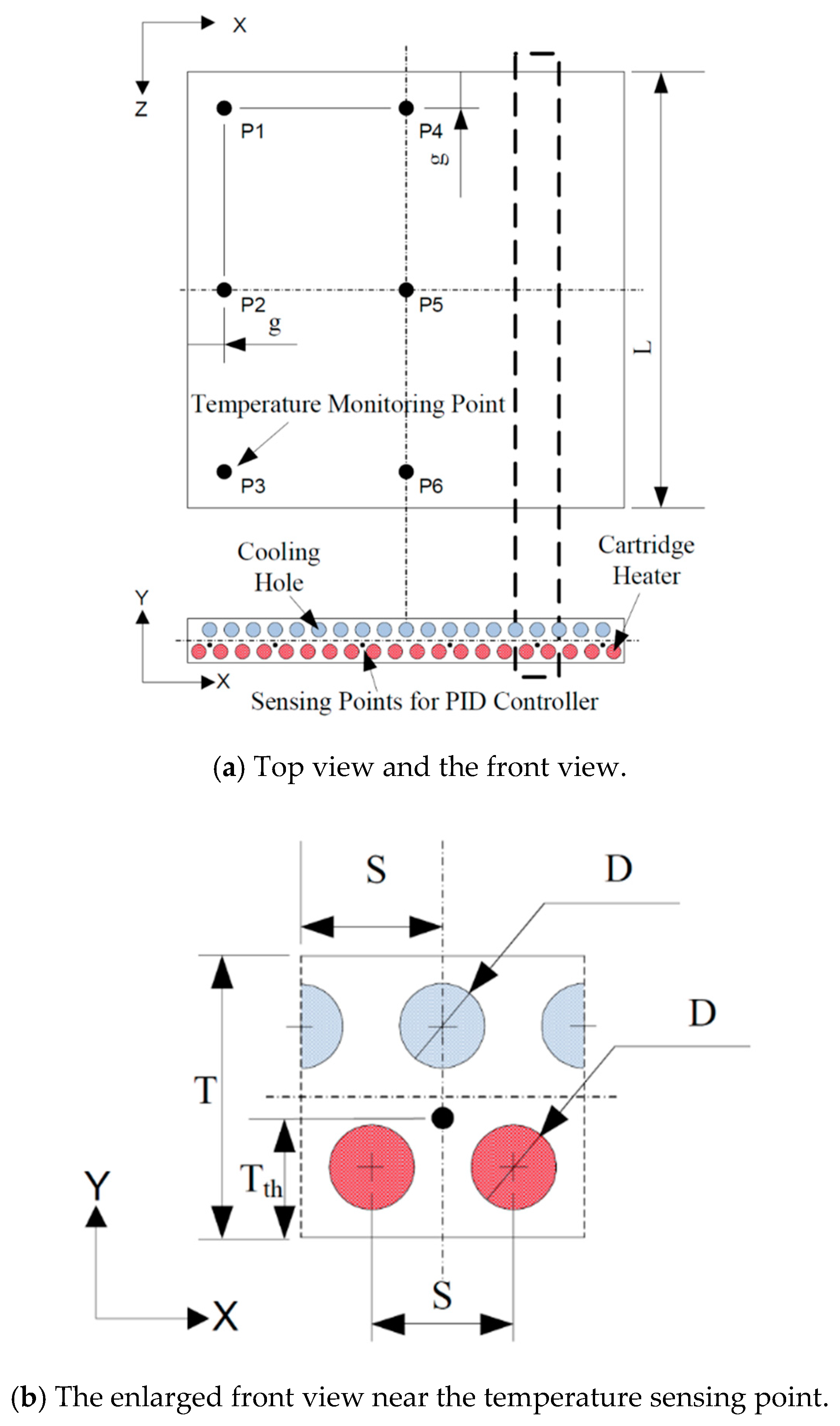
Figure 3 and Table 3 show the hot plate model for analysis. The cooling holes are located on the top of the flat hot plate and the circular cartridge heaters are mounted on the bottom. Heating is performed by the heat supplied by the heaters, while cooling uses the two different models as described above. This includes a direct cooling method in which the coolant flows in the cooling holes, and an indirect cooling method in which heat pipes longer than the hot plate are inserted into the cooling holes, and the heat pipes protruding outside the hot plate are cooled to indirectly cool the hot plate. Figure 3 shows the hot plate investigated in this study; the basic structure is the same as that of the previous study [9,10]. The hot plate is a square plate structure with a side length L and a thickness d. Excluding the outer edge of the hot plate with a width of g, the square area with a length of L-2g on one side is the area in which actual work is possible. On the side of the hot plate, circular holes with diameter D are vertically staggered in two rows in the longitudinal (z) direction. The holes are arranged horizontally at intervals of S, a key advantage of this hot plate enabling large-area expansion by increasing the number of circular holes.
As shown in Figure 3, the circular cartridge heaters are inserted into the lower circular holes to provide a heat source in the heating mode, and the upper circular holes are used for cooling. The main specifications of the hot plate used in this study are as follows. L = 240 mm, D = 6 mm, G =10 mm, d = 20 mm, S = 12 mm. On this basis, 20 cartridge heaters are mounted on the bottom and 19 cooling holes are processed on the top. The heating capacity per cartridge heater is 300 W. The hot plate uses a stainless-steel material STS304 with a density of 8030 kg/m3, and a thermal conductivity of 15.1 W/mK. The thermal diffusivity is 3.75 × 10⁻⁶ m2/s, much smaller than the thermal diffusivity of 7.10 × 10⁻⁵ m2/s of aluminum considered in the previous study.
This study considered two hot plate models with different cooling hole utilization methods. In Model I, as described in the previous study [8], the cooling holes are used as the passage in which the coolant flows only in the cooling mode to directly cool the hot plate. On the other hand, Model II inserts heat pipes in the cooling holes as a method of improving temperature uniformity, which may be insufficient in Model I. This model uses heat pipes longer than the hot plate; the end parts of the heat pipes protruding to the outside are cooled to indirectly cool the hot plate. The outer diameter of the heat pipe is 6 mm and the length is 340 mm. Here, the 30 mm portion at the end of the 100 mm portion protruding from the hot plate is cooled.
Feedback control is performed for the heat generation of the cartridge heaters so that the hot plate temperature can optimally approach the temperature setpoint and stabilize the system. As performed in the previous study [9], a total of 6 PID controllers were used to control the 20 heaters. As shown in Figure 3a, six temperature-monitoring points are arranged: two heaters near the temperature monitoring points of the outer frame are grouped into one group; four heaters near the inside temperature-monitoring points are grouped into six groups, for which independent temperature control is then performed.
2.3. Control Variables Setting
In the numerical experiment for setting the control variables, because the computational load would be large for the calculation of the entire area, we used a simplified model with a small partial analysis area as shown on the right side of Figure 3. For comparison with the experimental model, we performed numerical calculations on a small hot plate made of aluminum material. The length of the hot plate is 120 mm, the outer diameter of the heater is 60 mm, the heating target temperature is 240 °C, and the heating capacity of one cartridge heater is 150 W.
(1) Proportional gain effect
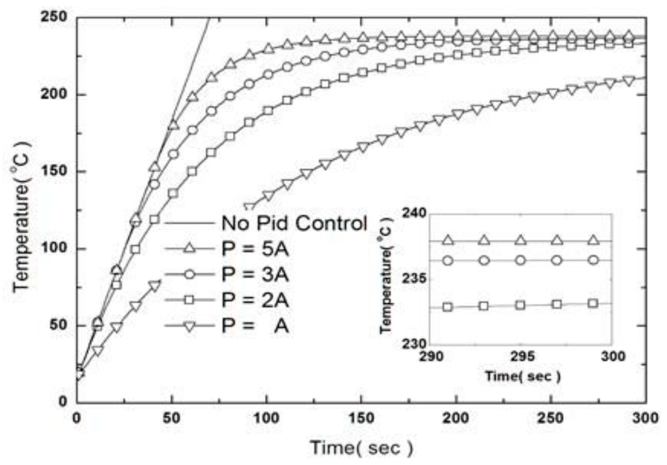
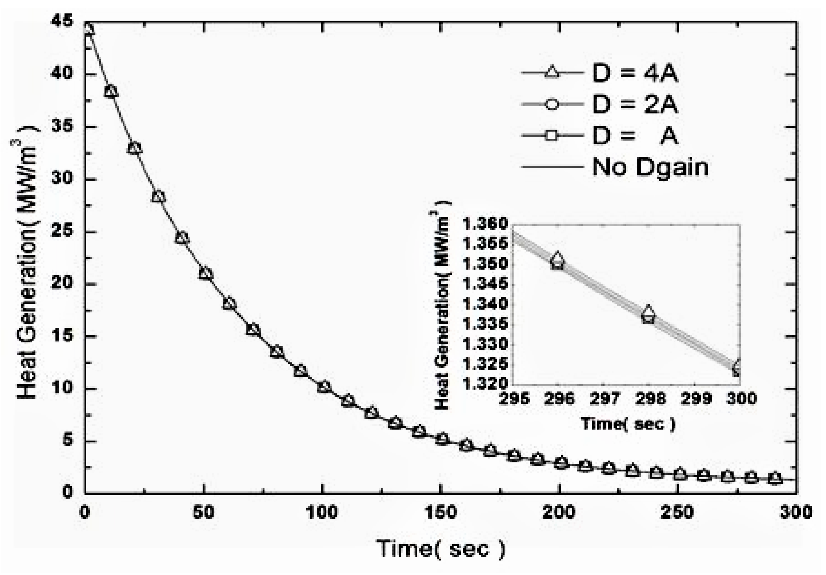
Figure 4 shows how the thermal behavior of the partial model varies with changes in the value of proportional gain. We set the integral gain and derivative gain of the partial model to zero and altered the value of proportional gain, creating a graph of the change in temperature over time obtained at the center of the hot plate. The lower right shows an enlarged section of the temperature curve from 290 to 300 s. Figure 5 shows the change in the heat generation per unit volume supplied to the cartridge heaters with time as proportional gain changes. The solid line in Figure 5 shows the temperature rise curve without control. The proportional gain value can be largely divided into four cases of -▽-, -□-, -○-, and -△-, with -▽- being the smallest. When the control was performed, up to 150 W of heat was set to be supplied to the cartridge heaters applied to the hot plate.
As the proportional gain increases, the temperature converges near 240 °C without rising above the target value; however, we confirmed that a constant value is maintained with the target value. The results show that even if the proportional gain (Pgain) increases, the overshoot phenomenon (overheating above the target value) does not occur, unlike behavior stemming from mass, elasticity, and damping due to vibration.
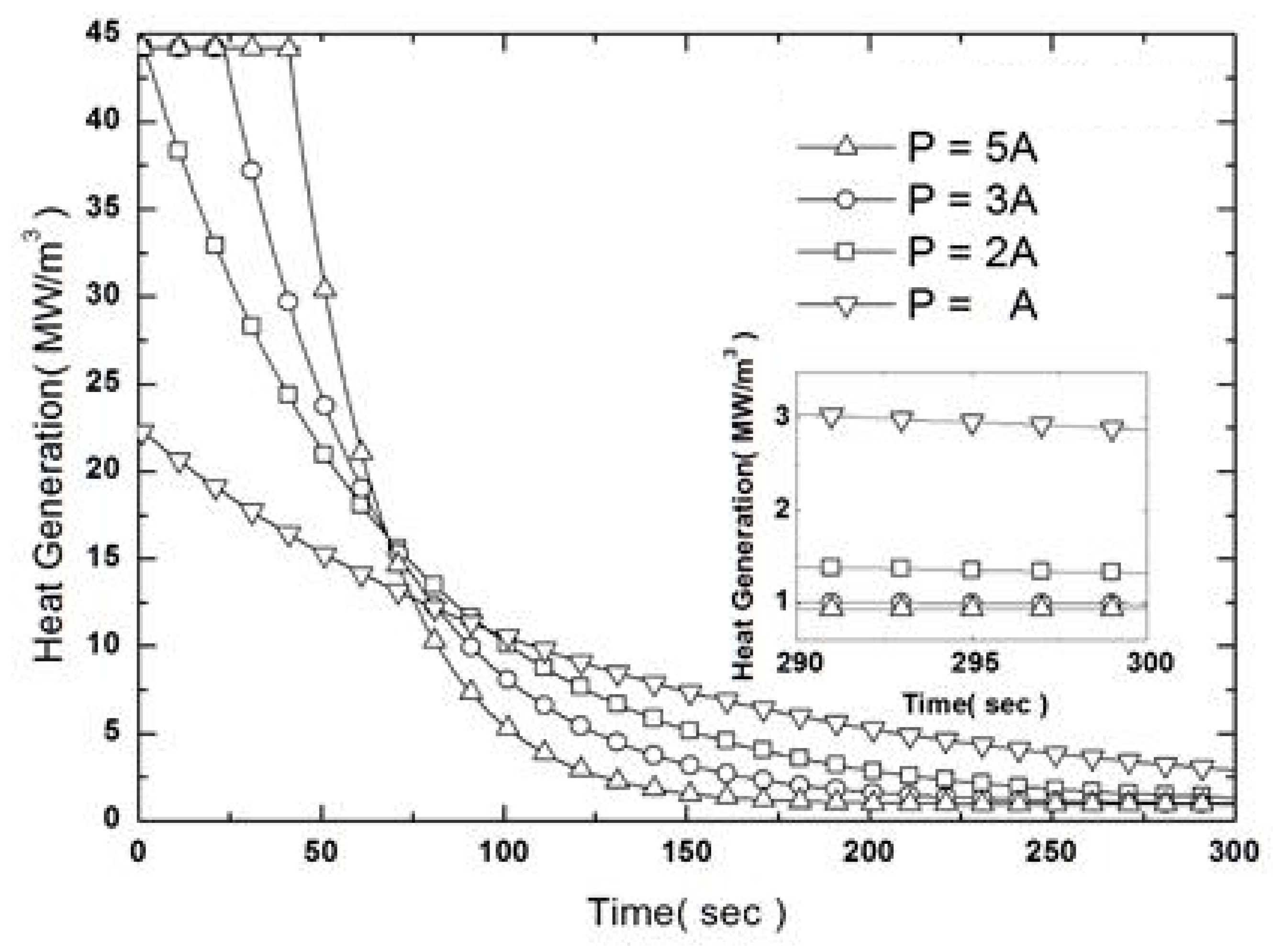
(2) Integral gain effect
Figure 6 shows the results of the numerical analysis experiment conducted according to changes in integral gain. Based on the previous experimental results, the graph shows the temperature behavior at the center obtained with variation in integral gain when the derivative gain is set to zero and the proportional gain is 5 A, which was determined as the optimal value. The lower right shows an enlarged section of the temperature curve from 290 to 300 s. Figure 7 shows the change in the heat per unit volume supplied from the cartridge heaters as the integral gain changes in the same manner.
The order of the symbols for increasing integral gain is -□-, -○-, and -Δ-. As in the unsteady analysis according to changes in proportional gain, the maximum heat supplied from the cartridge heaters applied to the hot plate is 150 W, equal to the heater specifications. If the integral gain applied to the symbol -□- is A, then this is applied 3 times to -○- and 5 times to -Δ-. Considering that the target temperature is 240 °C, we can confirm that as the integral gain increases, the temperature converges on 240 °C. For -Δ-, we observe a temperature of 240 °C or higher. Figure 7 shows that the heat supplied decreases between 290 °C and 300 °C also with a small gradient, indicating that control is still being performed. This phenomenon indicates that integral gain can be utilized to reduce the steady state error, that is, the difference between the target temperature and the measured temperature. Therefore, the target temperature of the hot plate can be controlled by simply using the proportional gain and the integral gain applied so far. We must additionally confirm whether derivative gain has an effect in order to confirm whether the simulation of PID control is feasible.
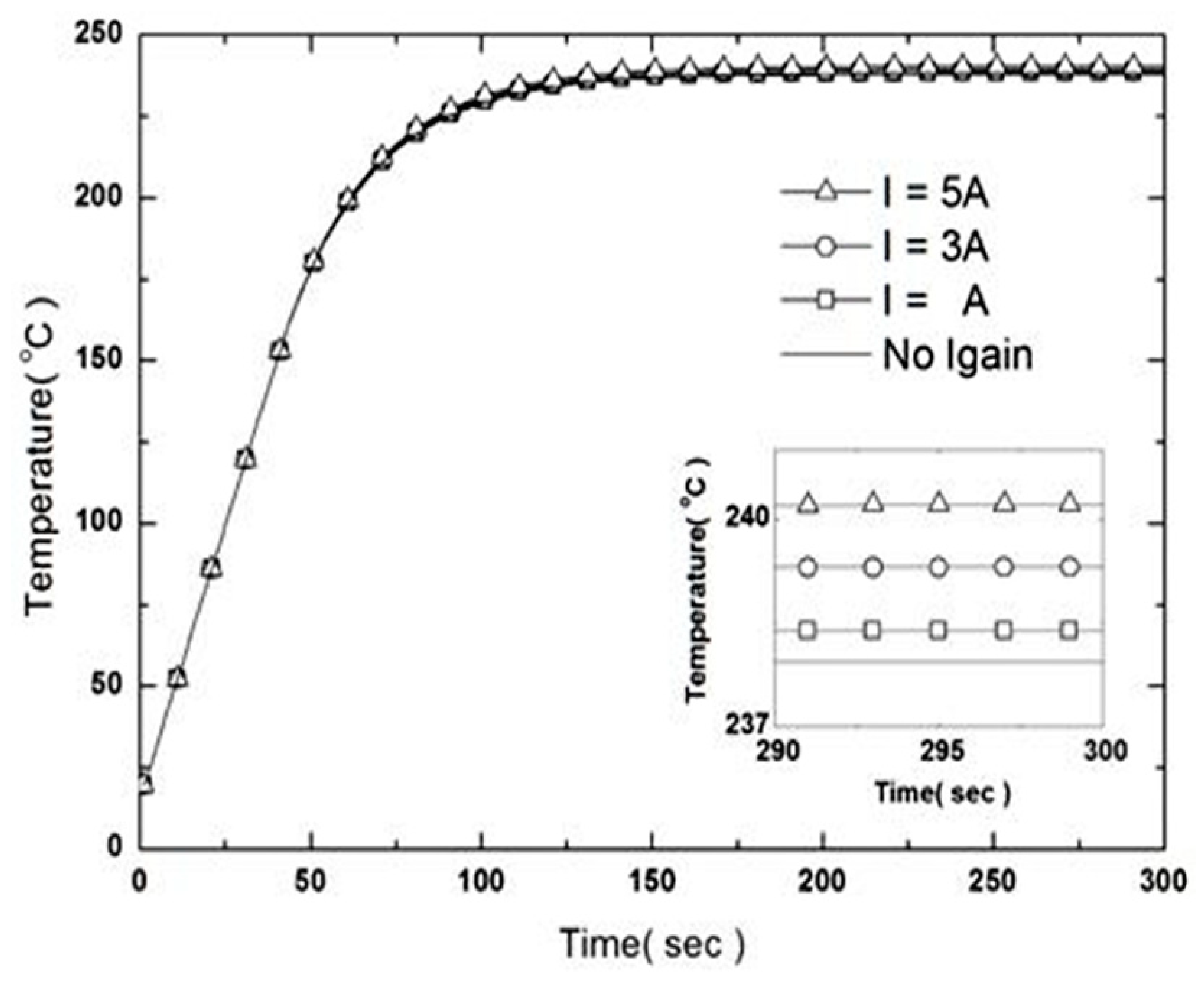
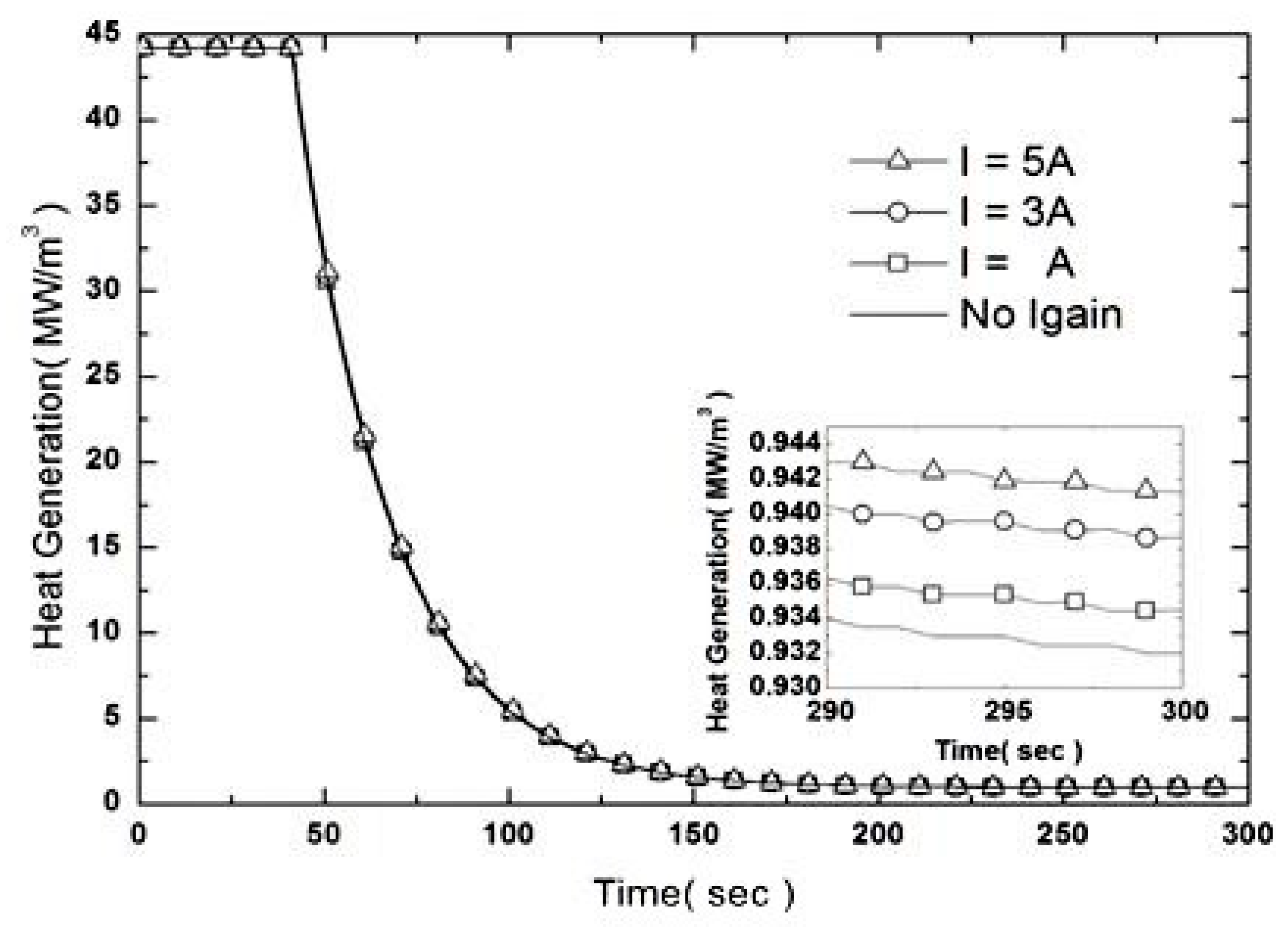
(3) Derivative gain effect
Figure 8 shows the temperature behavior of the hot plate according to changes in derivative gain. Figure 4 shows the temperature behavior at the center obtained with variation in derivative gain when the integral gain is set to zero and the proportional gain is 2 A. The lower right shows an enlarged section of the temperature curve from 295 to 300 s. Figure 7 shows the heat per unit volume supplied to the cartridge heaters according to variation in the derivative gain. The graph shows the derivative gain as a solid line for comparison with the case in which derivative gain is not applied (gain value of zero). The order of the symbols for increasing derivative gain is -□-, -○-, and -Δ-. The appropriate proportional gain should be applied to observe phenomena that may occur as the derivative gain increases. This is because it is difficult to observe the effect of derivative gain when proportional gain is small. Overshoot may occur if proportional gain is large. As derivative gain increases, the compensating value becomes larger and the tendency of approaching the target temperature becomes more prominent.
Figure 9 shows that at the same time as the heat per unit volume supplied from the cartridge heater, the amount of heat that is finely supplied increases after 300 s. However, Figure 8 shows that the temperature at the center of the heating plate decreases as the derivative gain increases. Here, control is performed from the start and the amount of supplied heat is reduced overall; however, as the temperature difference of the current time decreases in comparison to the temperature difference of the past time, the size of the entire supply decreases. Therefore, the effect of increasing the derivative gain becomes greater. We confirmed that as the derivative gain increases, the final temperature decreases gradually. However, as shown in the lower right of Figure 6, the increase in temperature is not large compared to the case without the derivative gain, indicating that the effect of derivative gain is included in the characteristics of the system. Furthermore, as mentioned in the previous section, the integral gain can be used to reduce the error of the steady state, suggesting that the present system can be controlled without applying the derivative gain. Accordingly, we analyzed the effects of proportional gain, integral gain, and derivative gain applied to the PID controller and verified the gain characteristics according to variations in each gain value.
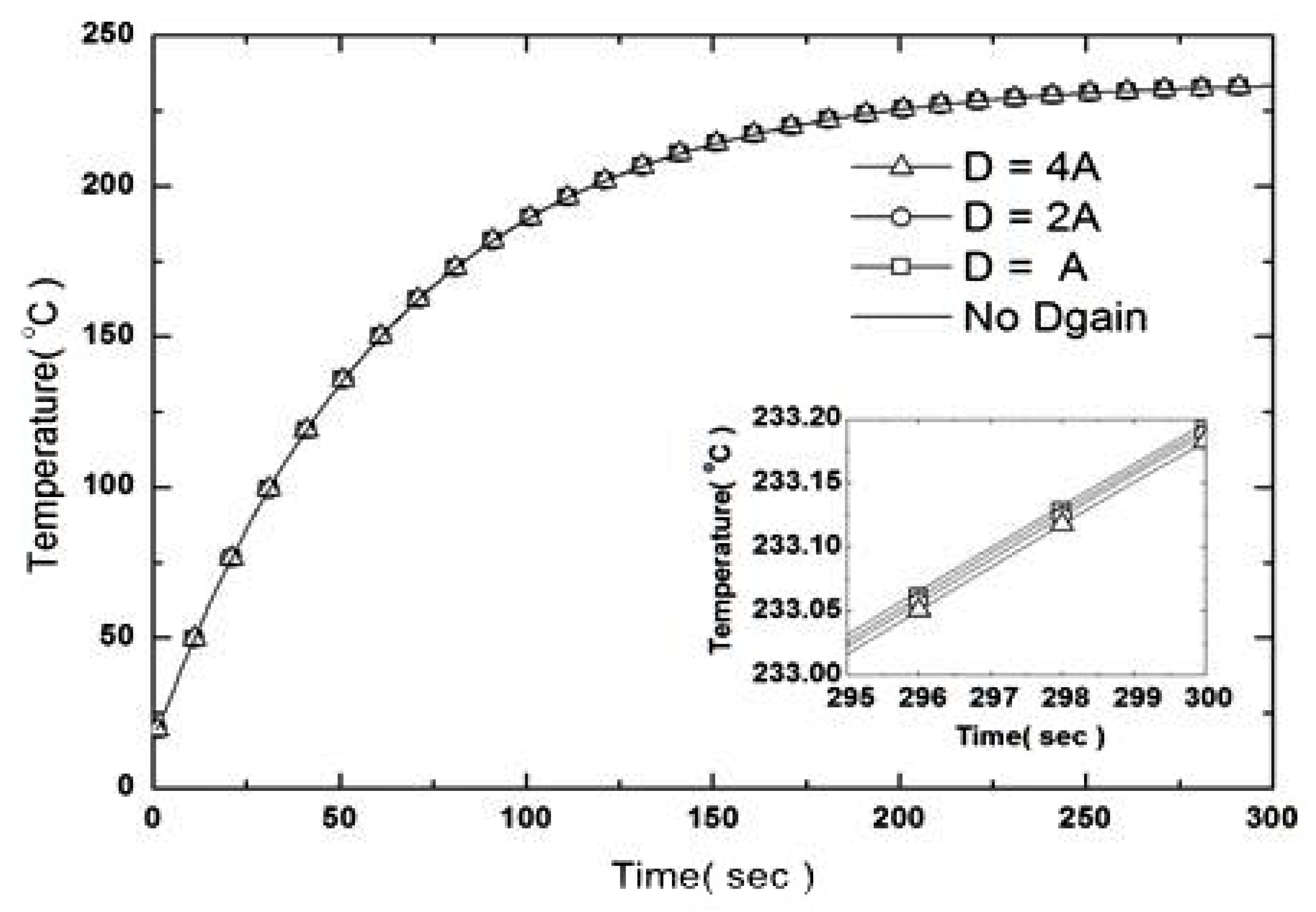
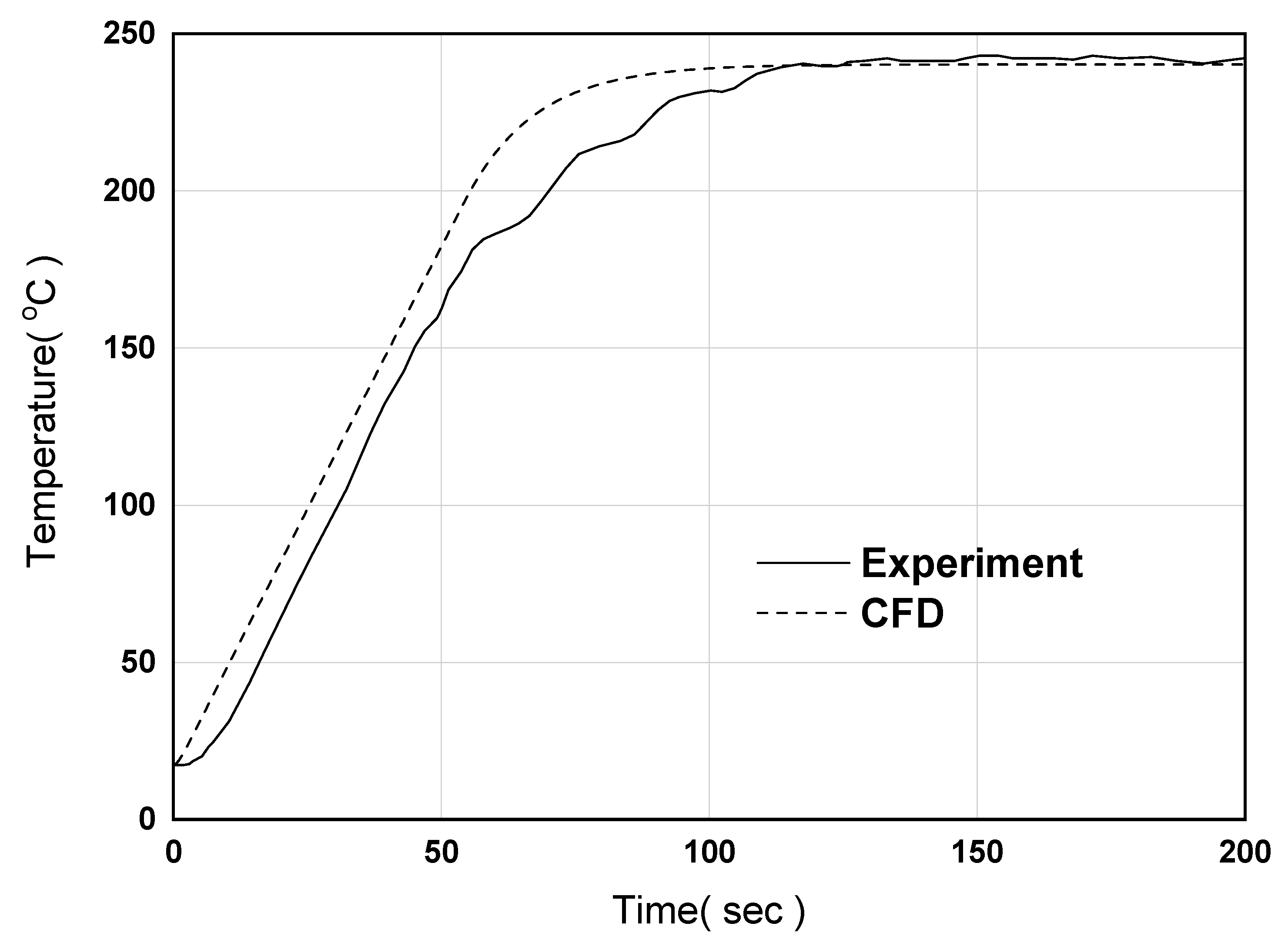
Next, to derive similar results to the actual experiment, we must select the gain value for computational analysis. In this study, as mentioned in the previous section, only the proportional gain and integral gain were applied, and the derivative gain was not. We selected the proportional gain and integral gain to reduce the steady state error. Figure 10 shows the temperature of the center obtained by applying PID control, as well as the experimental results obtained through automatic tuning. It is noteworthy that between 0 and 10 s at the beginning, the temperature slowly increased in the experiment whereas it sharply increased in the computation. This phenomenon can be attributed to the required initial start-up time according to the power supply at this time.
3. Results and Analysis
3.1. Heating Numerical Analysis Characteristics
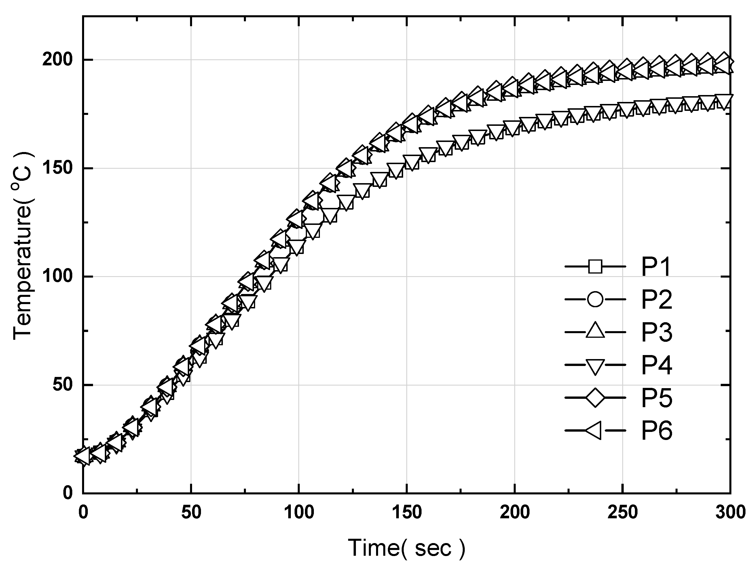
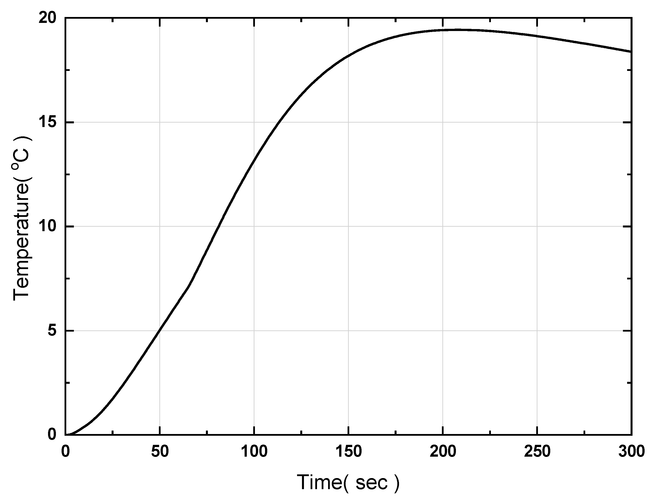
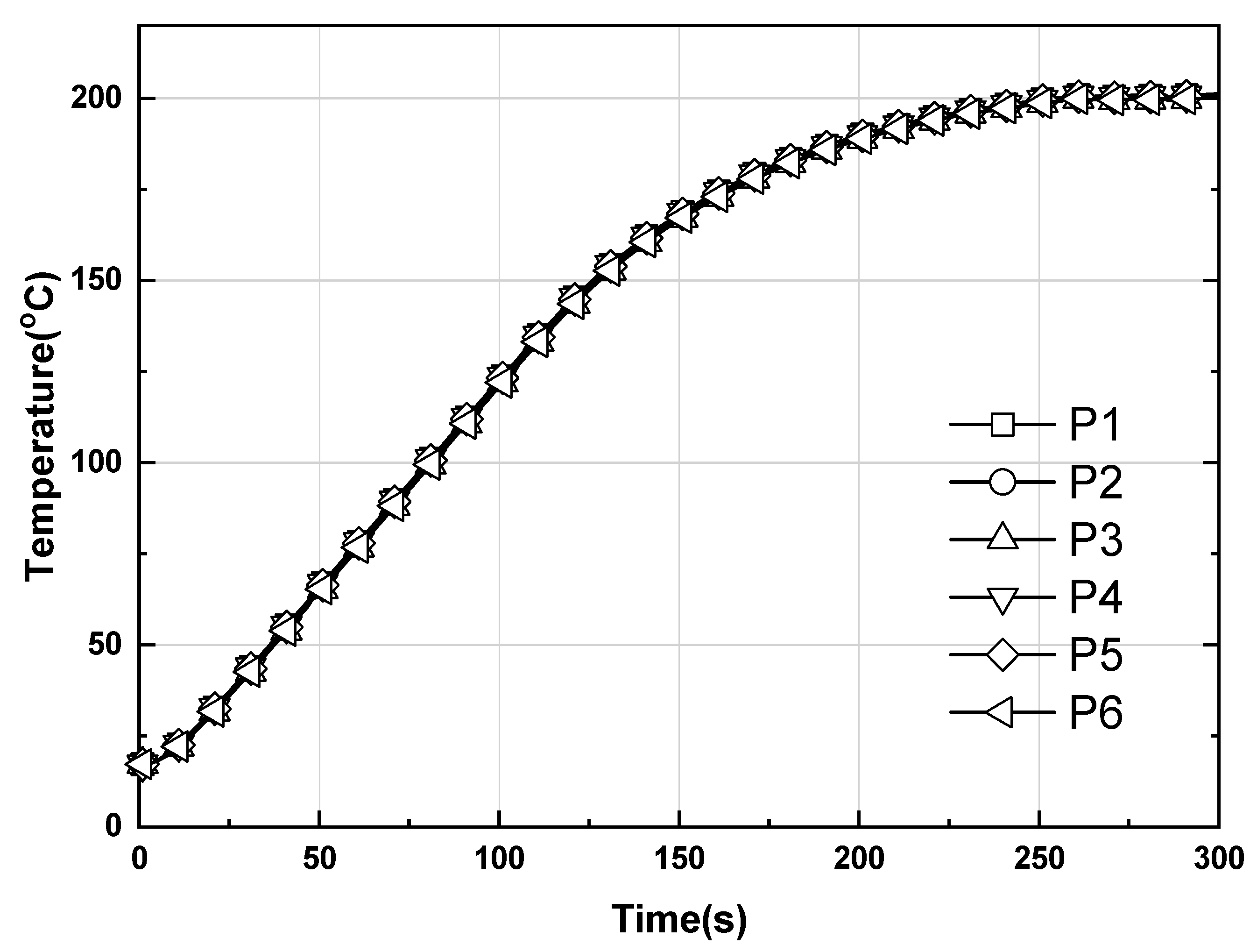
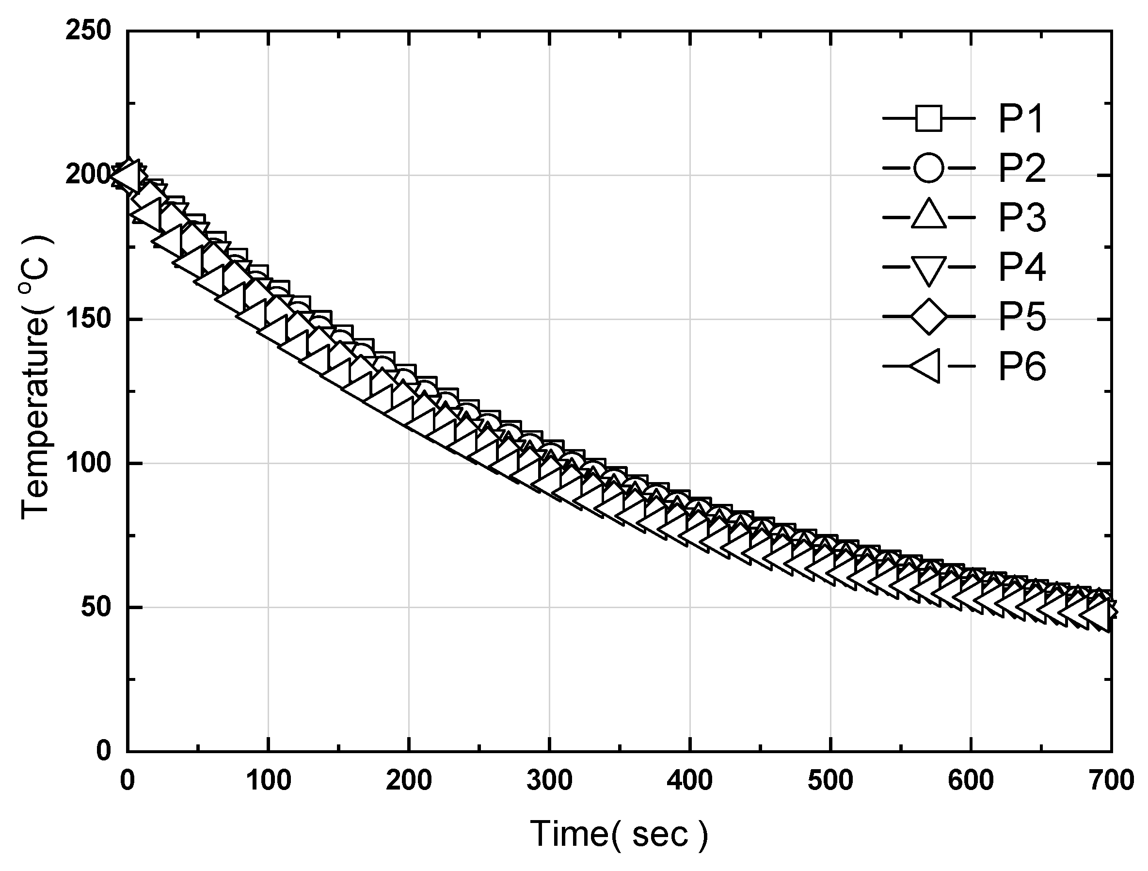
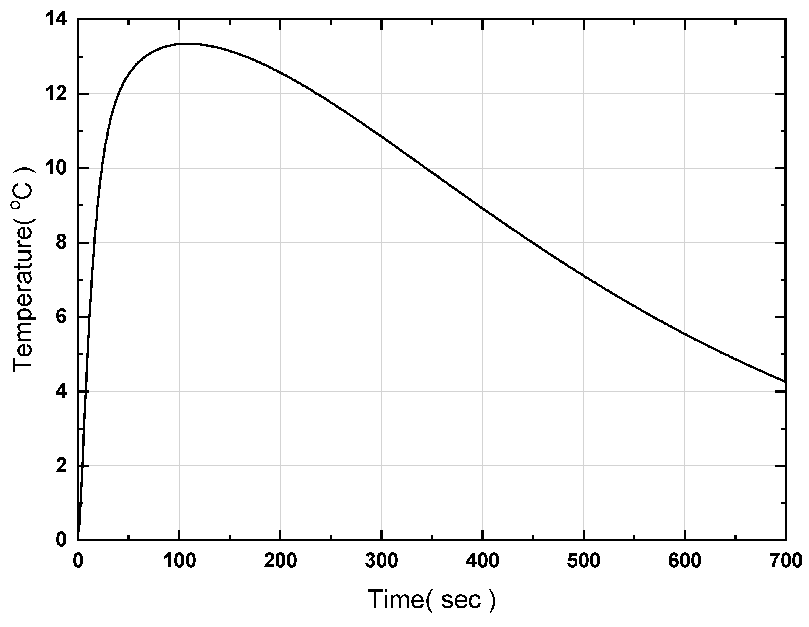
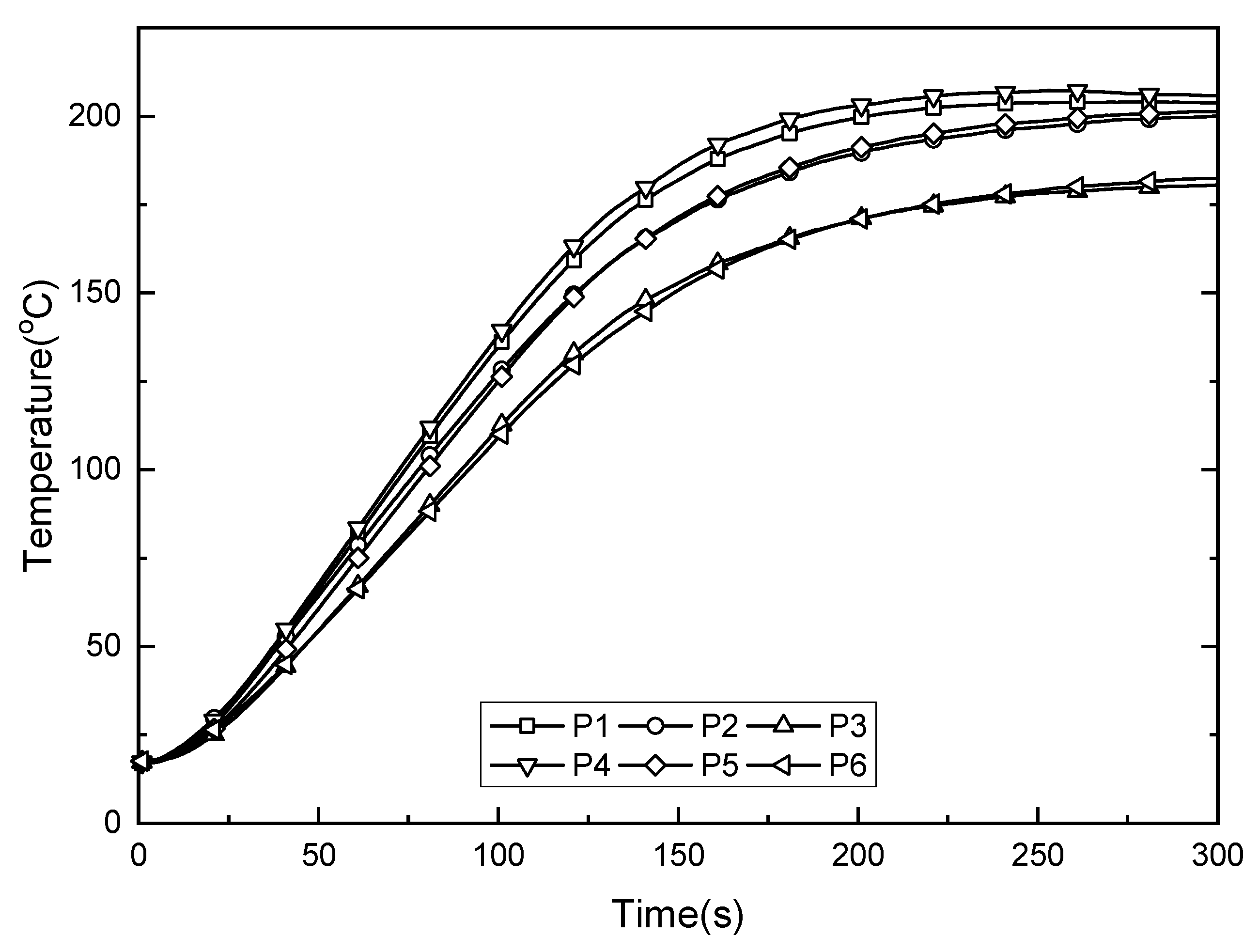
Figure 11a,b show the temperature changes at the center of the hot plate with PID control applied for one sub zone mentioned in Figure 3. Through a computer simulation of the PID controller using a small model, we confirmed that the roles of Pgain and Igain are dominant. Thus, when using a large-area hot plate as well, as the area widens, the heat supplied increased on the sides of the hot plate compared to a smaller one. Nevertheless, as the density corresponding to the heat storage capacity does not differ, the Dgain effect is also not significantly different. Accordingly, we analyzed the performance of the controller based on Pgain and Igain for the submodel. Because the system characteristics for the large-area hot plate differ, the gain value of PID control obtained through the computer simulation of the small hot plate must be re-selected. Figure 11a shows four examples of temperature behavior according to variations in Pgain during PID control. The target temperature of the hot plate was set at 200 °C. -○- represents the temperature curve at the center of the hot plate obtained by experiment rather than computational analysis, while -□- indicates the case in which PID control is not performed. Otherwise, the order of the symbols for increasing Pgain is -△-, -▽-, and -◇-. -△- is the smallest value of Pgain; if the applied Pgain is A then this is increased by three times to -▽- and 100 times to -◇-. In the computational analysis, the control time was 0.5 s. At the beginning of the temperature curve, the temperature of the heater itself increases when power is supplied to the cartridge heaters and an initial start-up time is required, resulting in a time delay and then a linear increase. When PID control is not applied, 300 W is supplied per heater; hence, as shown by -□-, the gradient of the temperature curve does not change due to the constant heat flux condition, and the temperature continues to increase. -Δ-, the smallest Pgain value, does not reach the target temperature of 200 °C because the power supplied to the heater is within the allowable power range. This was confirmed to be small compared to the solid line in which PID control is not performed. As Pgain increases, the temperature maintains a constant gradient and then approaches 200 degrees; the difference to the target temperature decreases, and is then maintained at approximately two to three degrees. The value of Pgain applied to control was selected to satisfy the same gradient with a time width of less than 0.2 degrees, based on the solid line case in which control was not applied. Figure 11b shows the temperature behavior according to variation in Igain in the steady state similarly applying the -▽- Pgain value (Pgain = 3 A) of Figure 11a to reduce the steady-state error. The order of the symbols for increasing Igain is -○-, -△-, -▽-, and -◇-. The steady-state error decreases as Igain increases, consistent with the experimental values. These results show that overshoot does not occur in the temperature behavior of the given hot plate and that the temperature of the hot plate does not fluctuate significantly, unlike the displacement control. This demonstrates that, as in the computational analysis, the role of Dgain is unnecessary in PID control. The values of Igain used in control were applied to satisfy a range of steady-state error of ± 0.02 °C. Figure 12 shows the temperature at each measurement point with no heat pipes and only the controller and hot plate. Measurement point P5 is located at the center of the hot plate and the rest are located 2 cm from the end. P1, P2, and P3 are located on one straight line in the longitudinal direction, while P4, P5, and P6 are located on another straight line. Overall, P1 and P4 show low temperatures, while the other measurement points show temperatures in the same position. P1 and P4 are low because heat is not generated 2 cm from the end of the cartridge heaters. To quantitatively analyze the temperature results, Figure 13 shows the difference between the maximum and minimum temperatures. As shown, the maximum temperature difference is 20 °C. This suggests that, considering the embossing process of the hot plate material, additional supplementary measures are needed to ensure temperature uniformity for large-area hot plate expansion when applying a stainless steel (STS304) material with a low thermal conductivity.
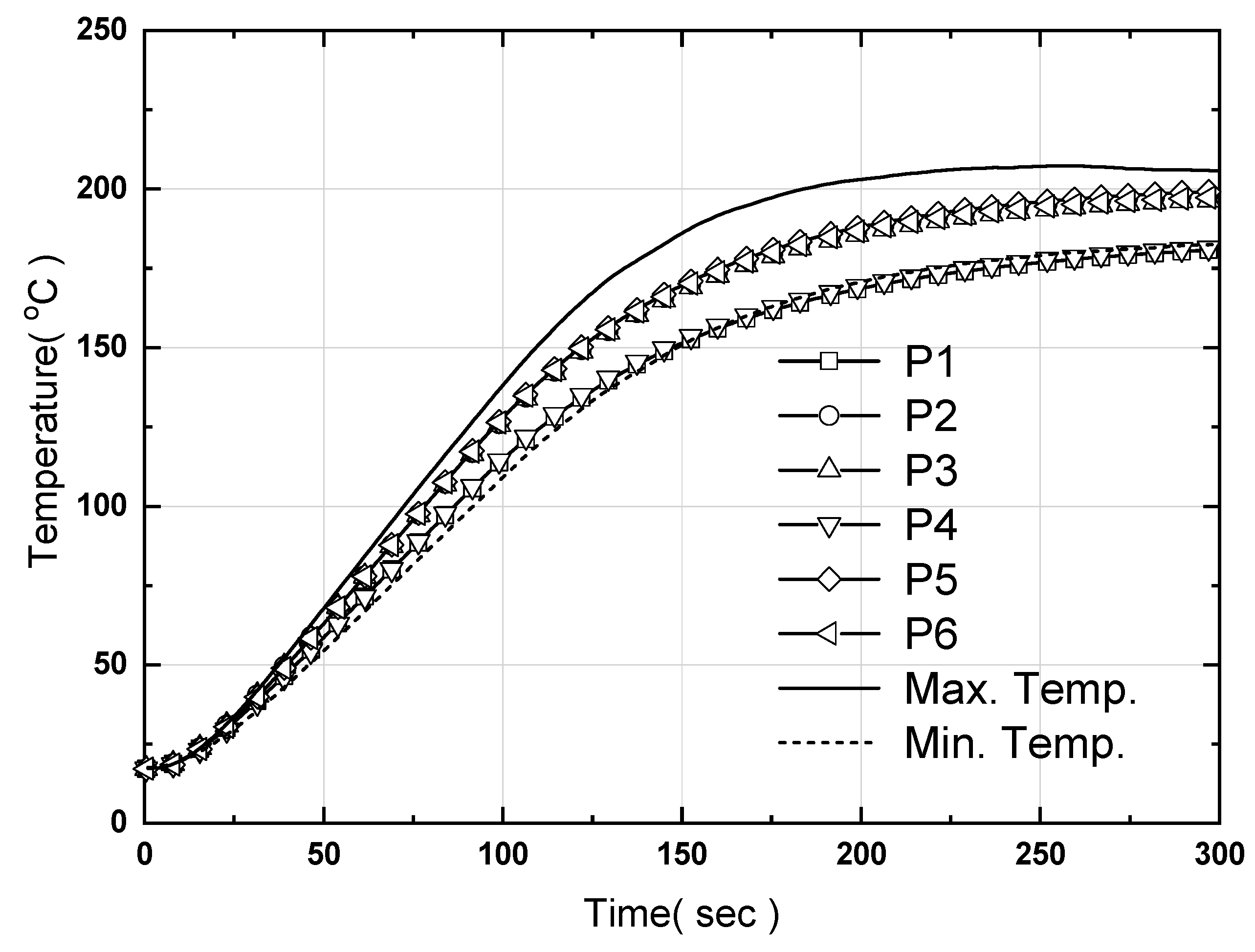
To reduce the temperature difference, Figure 14 shows the thermal behavior of the work surface with time when control is performed using heat pipes with a diameter of 6 mm and length of 340 mm, the same manner as the hot plate model in Figure 3. The measurement points are the same as in Figure 3a, and the thermal conductivity of the heat pipes was 80 times that of copper. When the heat pipes are applied, the temperature uniformity of the hot plate is maintained at 200 ± 1 °C. The rate of heating increase was 40 °C /min. This result indicates that temperature uniformity can be improved by using heat pipes even when the hot plate is made from stainless steel (STS304).
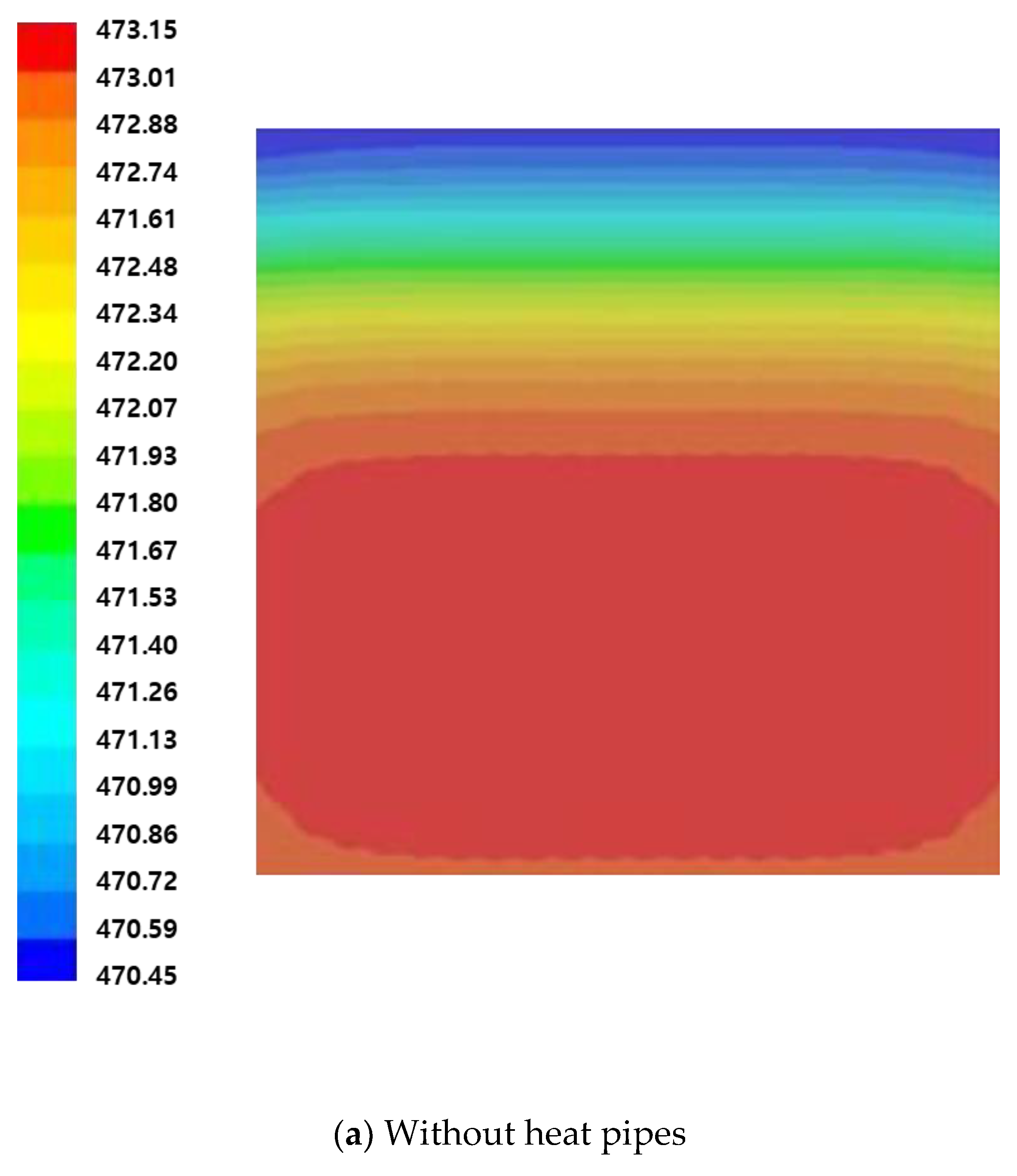
Figure 15a,b shows the temperature field above the hot plate after 300 s of heating. Figure 15a shows the case without heat pipes, and Figure 15b shows the case with heat pipes. Without heat pipes, the temperature difference in the z-axis direction in which the cartridge heaters are inserted is larger than that in the x-axis direction. The model mirroring the actual experiment showed that heat was not generated in the 20 mm end part of the cartridge heaters. This confirms that the temperature of the center is high due to the heat superposition phenomenon. In the case with heat pipes, the heat is relatively evenly distributed and the difference in temperature is maintained within three degrees.
3.2. Cooling Numerical Analysis Characteristics
Figure 16 shows the temperatures measured at the six points in the case without heat pipes after turning on counter-directional nitrogen cooling flows in the cooling holes with a length of 240 mm, while Figure 17 shows the difference between the maximum and minimum temperatures for the same. The speed of the coolant was set to 10, 20, and 30 m/s as before. Counter-directional cooling was applied due to its superiority for single-directional cooling. The temperature decreases as the speed of the coolant increases; however, as the difference between the maximum and the minimum temperatures ranges from 17.5 °C to 20 °C, the cooling method using nitrogen is still problematic.
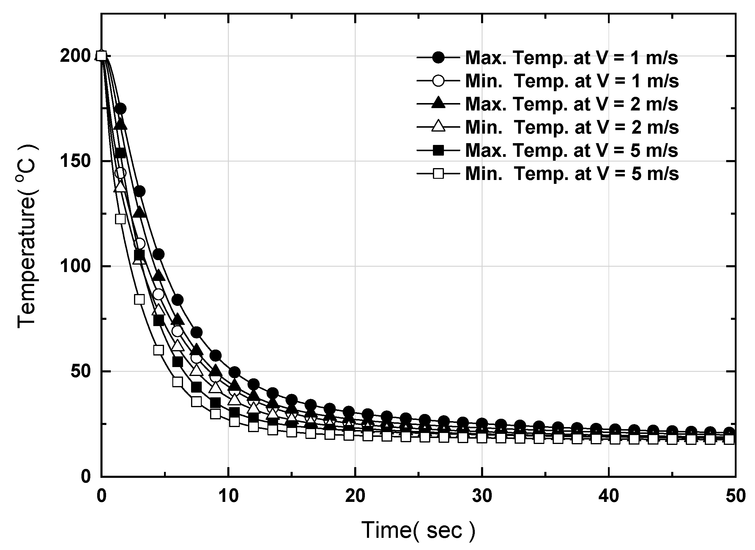
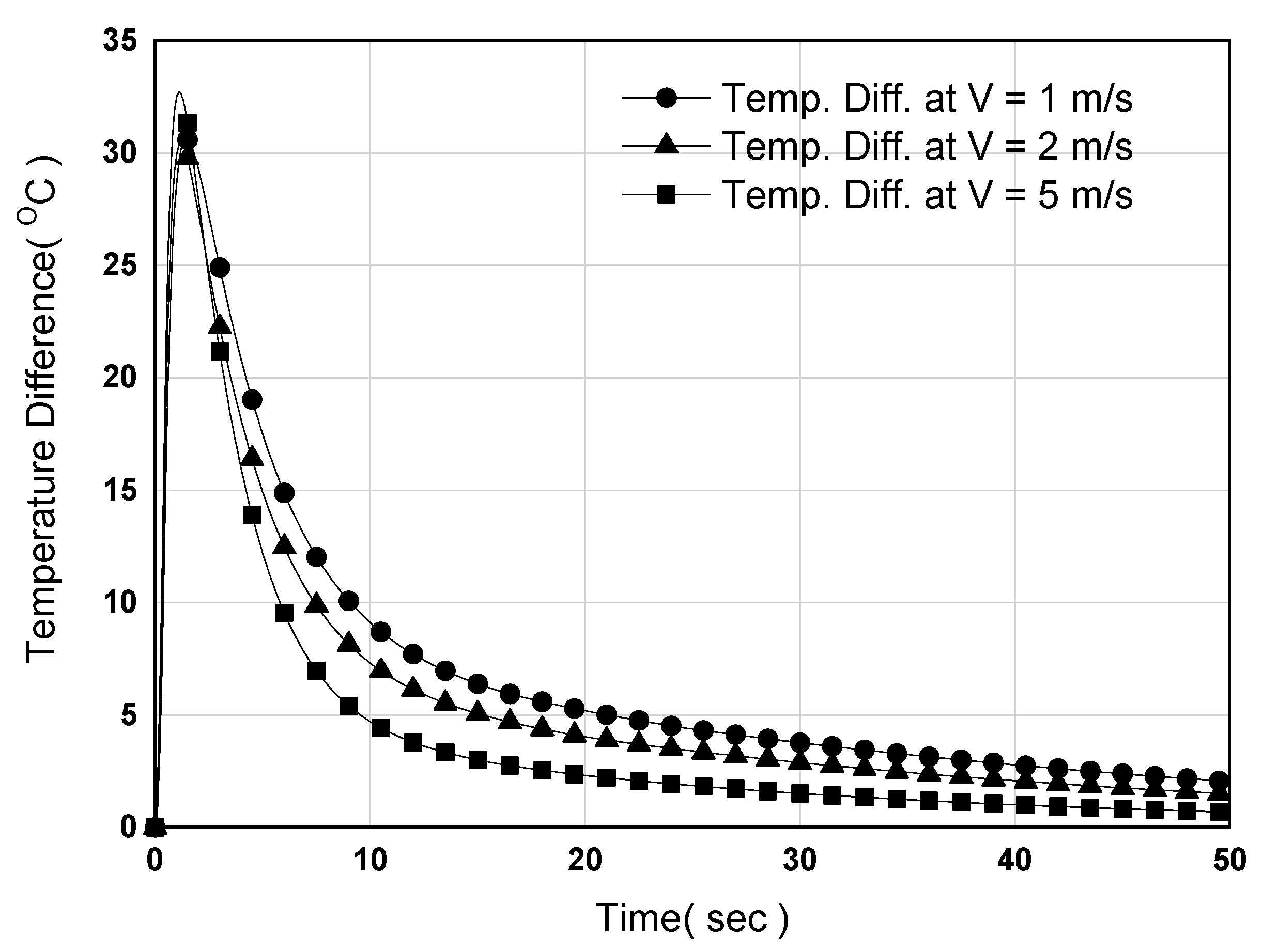
Figure 18 and Figure 19 show the maximum and minimum temperatures as well as the temperature difference when water is used as the coolant in counter-directional cooling. The speed of the coolant was 1, 2, and 5 m/s, the actual rates available on semiconductor equipment production lines. As with the cooling method using nitrogen, the temperature difference decreases as the coolant speed increases; furthermore, the cooling time was reduced compared to the nitrogen method. However, with a maximum temperature difference of 30 °C or more, it would take approximately 20 s to fall below 5 °C. This indicates that issues may arise in cooling when using water as a coolant as well. Therefore, the hot plate cannot be directly cooled using a coolant, and a different method is required. We also confirmed the need to secure temperature uniformity in order to expand the hot plate into a larger area. To solve this problem, the heat pipes were also applied to cooling.
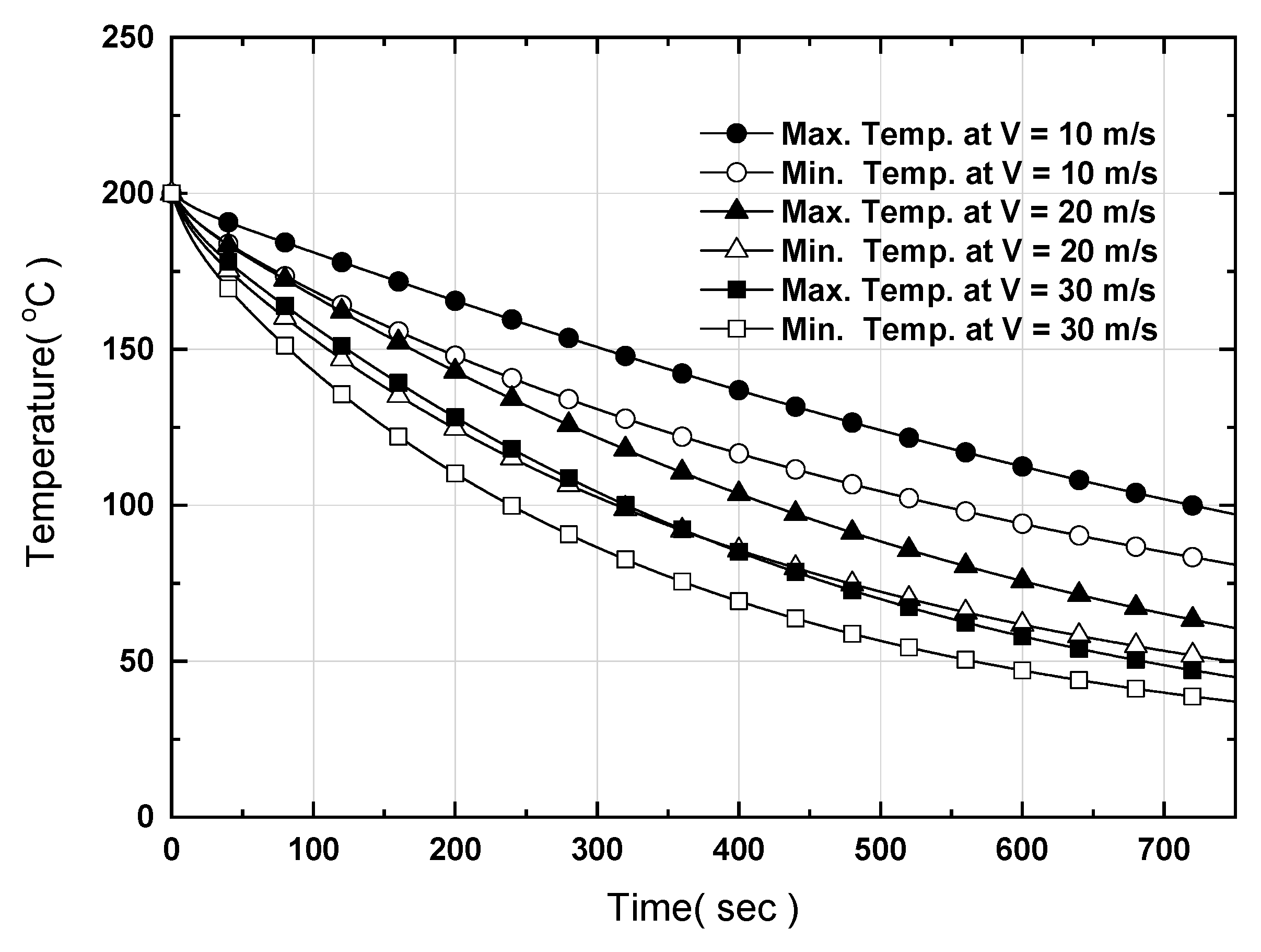
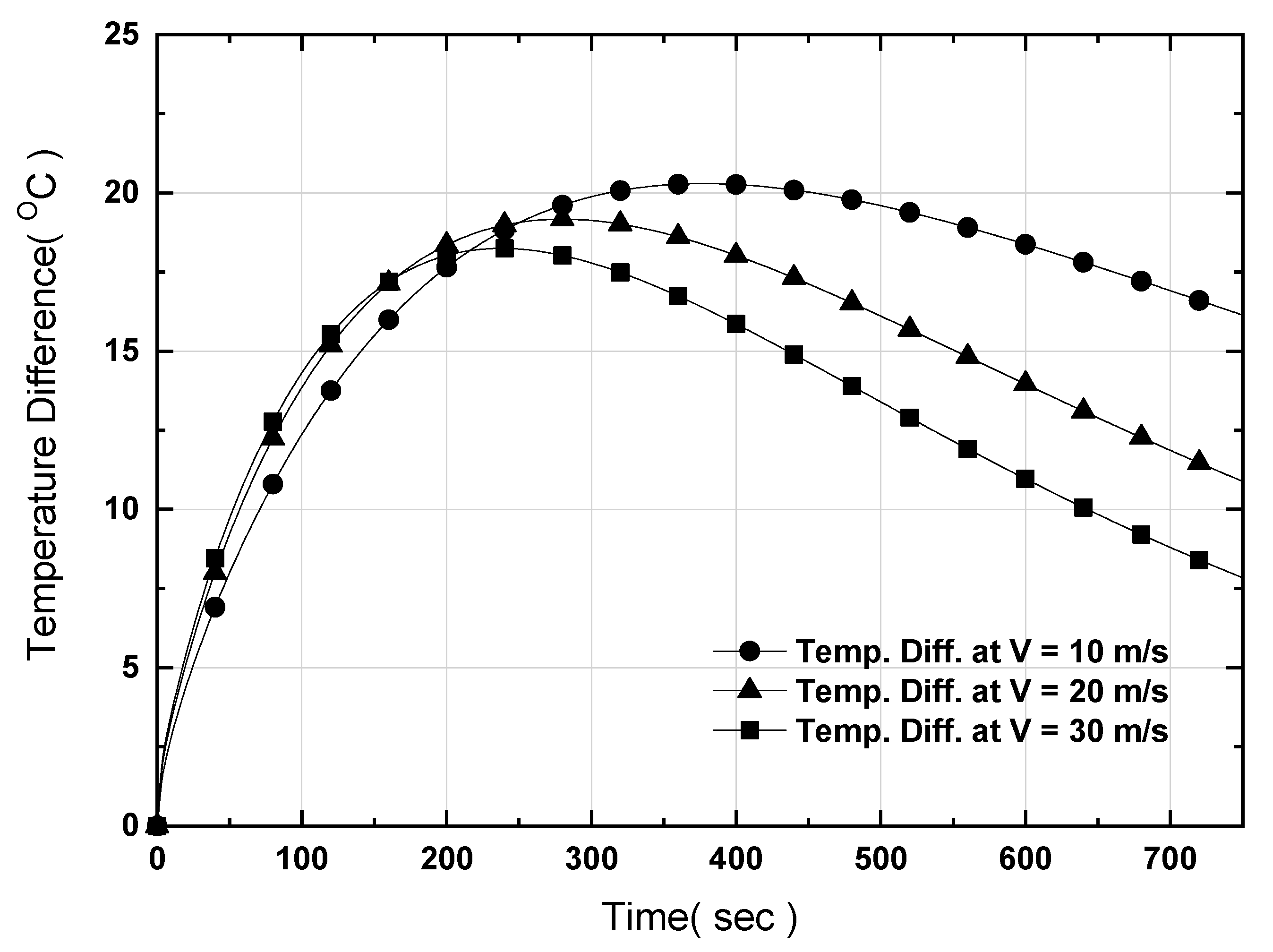
Figure 20 shows the unsteady temperature behavior from the temperature monitoring points P1 to P6 (Figure 3a) when the end 20 mm is cooled with air at 15 °C. The flow rate of the air is 30 m/s. The heat transfer coefficient, a boundary condition, was evaluated at 1768.4 W/m2K through Equation (3) using the derived convection heat transfer coefficient based on a processing capacity of 150 W (the processing capacity of the heat pipes). The heat pipes were modeled with a thermal conductivity of 80 times that of copper; thus, as cooling was performed via convection, the temperature curve showed a monotonically decreasing pattern overall. Additionally, when the glass transition temperature is set to 100 °C (105 °C for polymethyl methacrylate (PMMA)), a cooling gradient of 20 °C/min was achieved, thereby satisfying cooling performance. Figure 21 shows the difference between the maximum and minimum values for quantitative evaluation. As the cooling time increases, the temperature difference is greatly reduced from 32.5 °C to 13.2 °C, unlike the cooling characteristics of the hot plate without heat pipes. Thus, temperature uniformity was improved.
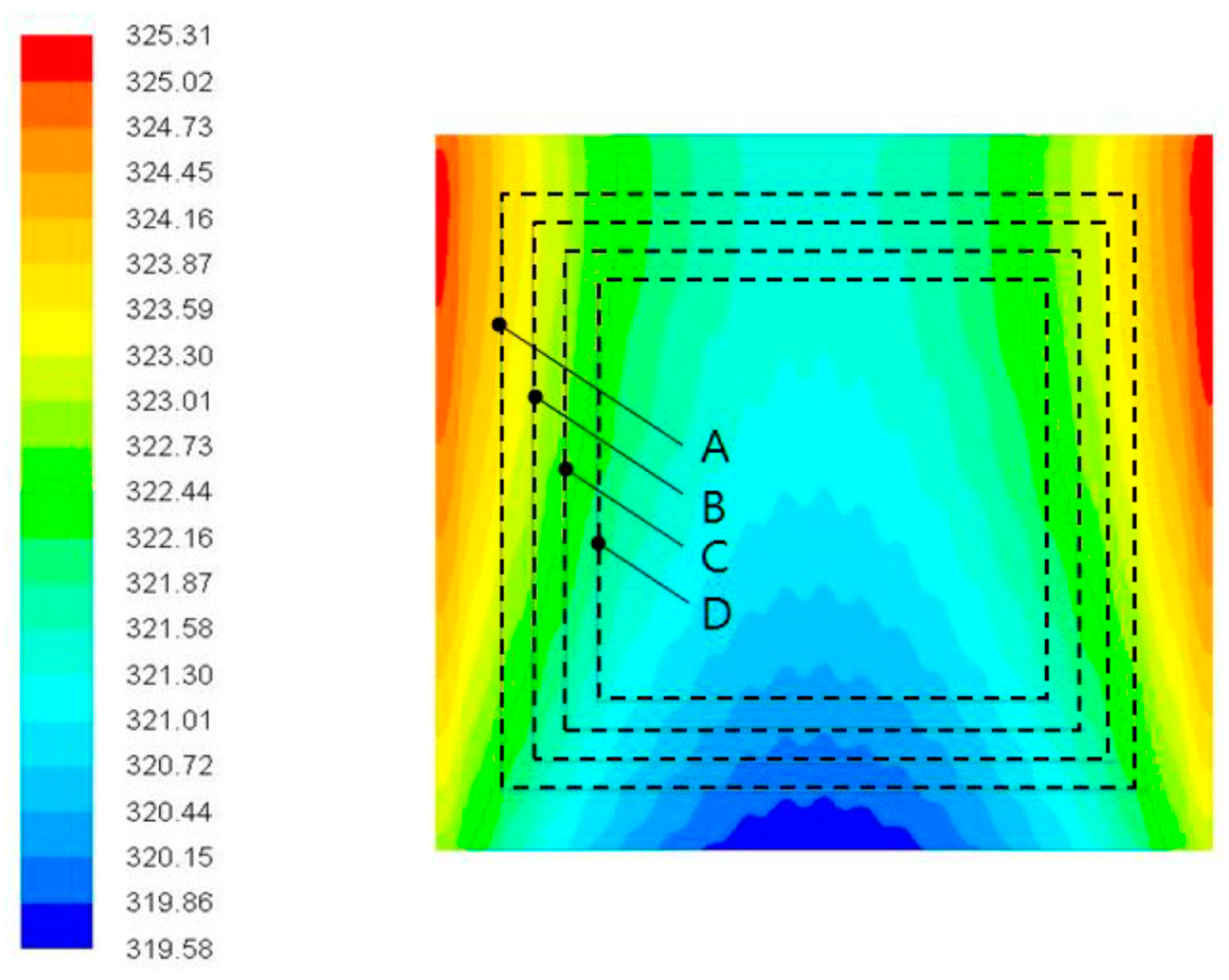
To analyze the possible working area of the entire hot plate, Figure 22 and Figure 23 show the temperature field of the upper surface 100 and 700 s after cooling. The heat pipe is positioned in the longitudinal (z) direction as shown in Figure 3. The cooling from the sidewall is not smooth, and cooling is fast at the center where the heat pipes are located. We confirmed that the area satisfying the temperature deviation ± 3 °C was 170 × 170 mm, under the current boundary conditions. Additional studies are needed to account for the available working area compared to the total area.
3.3. Comparison of Numerical and Experimental Results
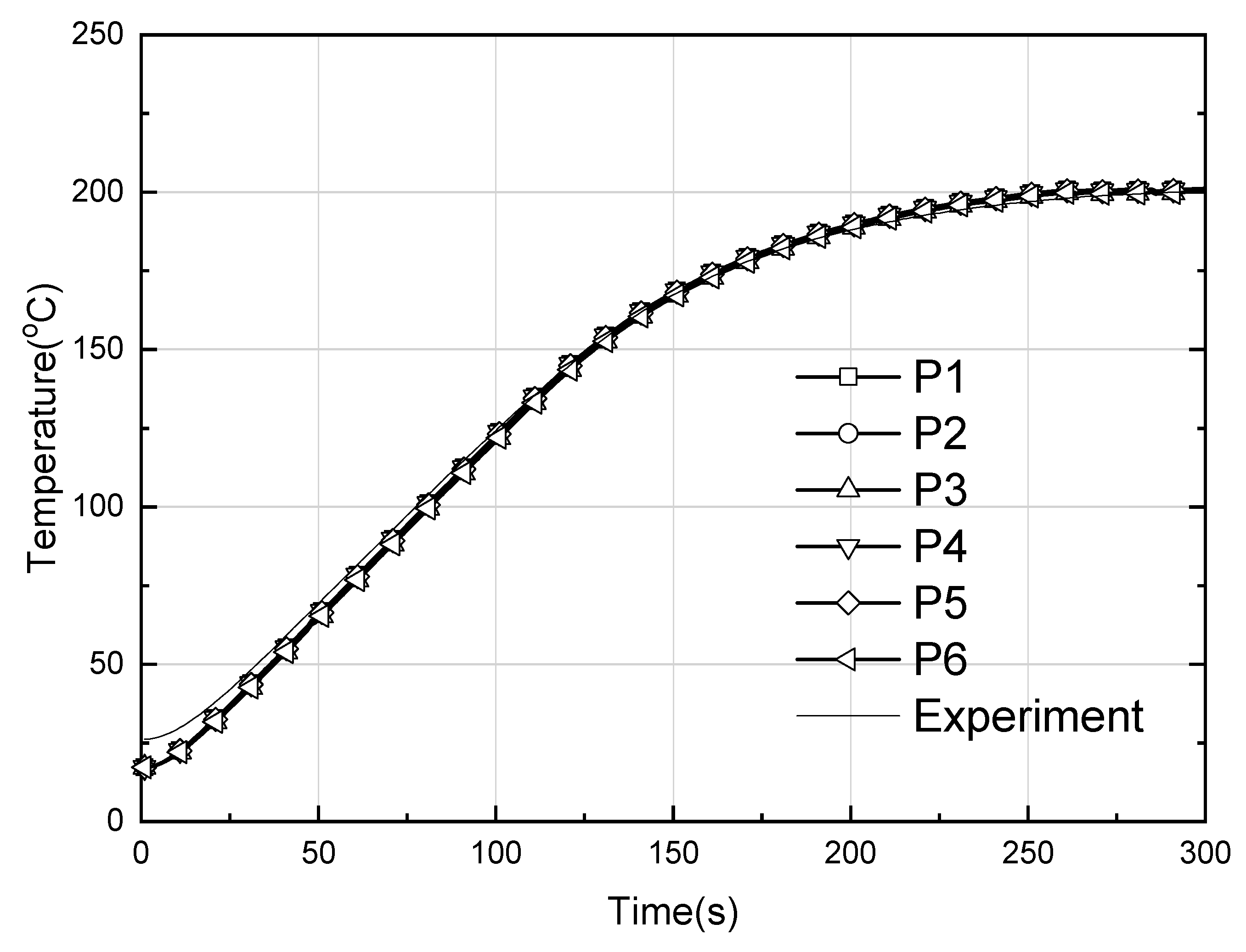
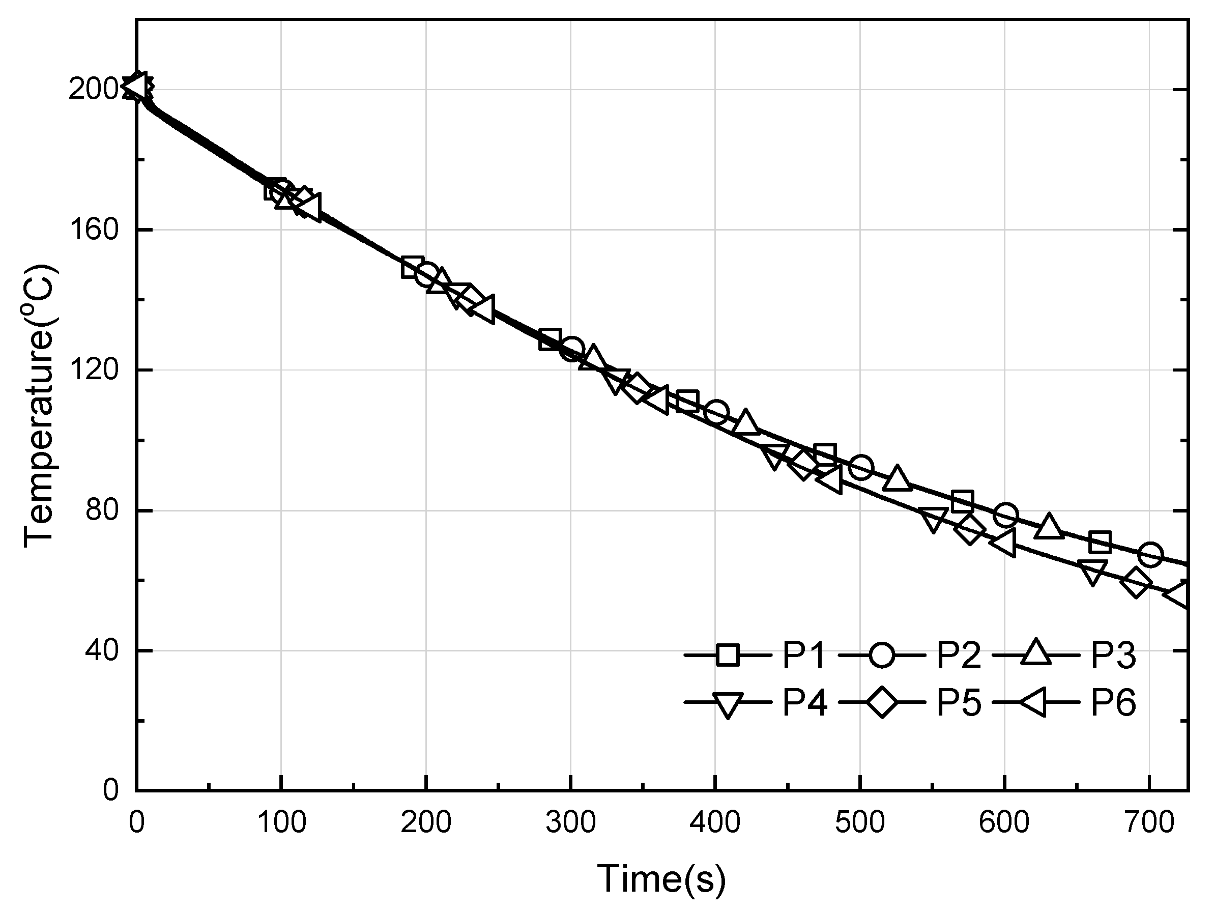
For the heating and cooling models, a computational analysis on a large-area hot plate using a hot plate model with a controller for heating, and a hot plate cooling model with heat pipes for cooling, was performed in this study. We compared the computational results and experimental results of Yang [31]. Figure 24 shows the unsteady temperature behavior of the hot plate with no heat pipes, as conducted by Yang. Figure 25 shows the maximum and minimum values, as well as those derived from the present calculations. Similar trends were shown overall. In the experiment of Yang [31], heat generation from the cartridge heaters did not occur at points P3 and P6, while this was observed at points P1 and P4 in the computational analysis. The increasing tendency of the temperature gradient can be attributed to the difference in gain value of the PID controller.
Figure 26 shows the unsteady temperature behavior during heating when heat pipes are used. The experimental and analytical results showed similar trends overall. The initial gradients differ due to the different initial start temperatures, but the same gradient was observed between 50 and 100 s when the maximum output occurs.
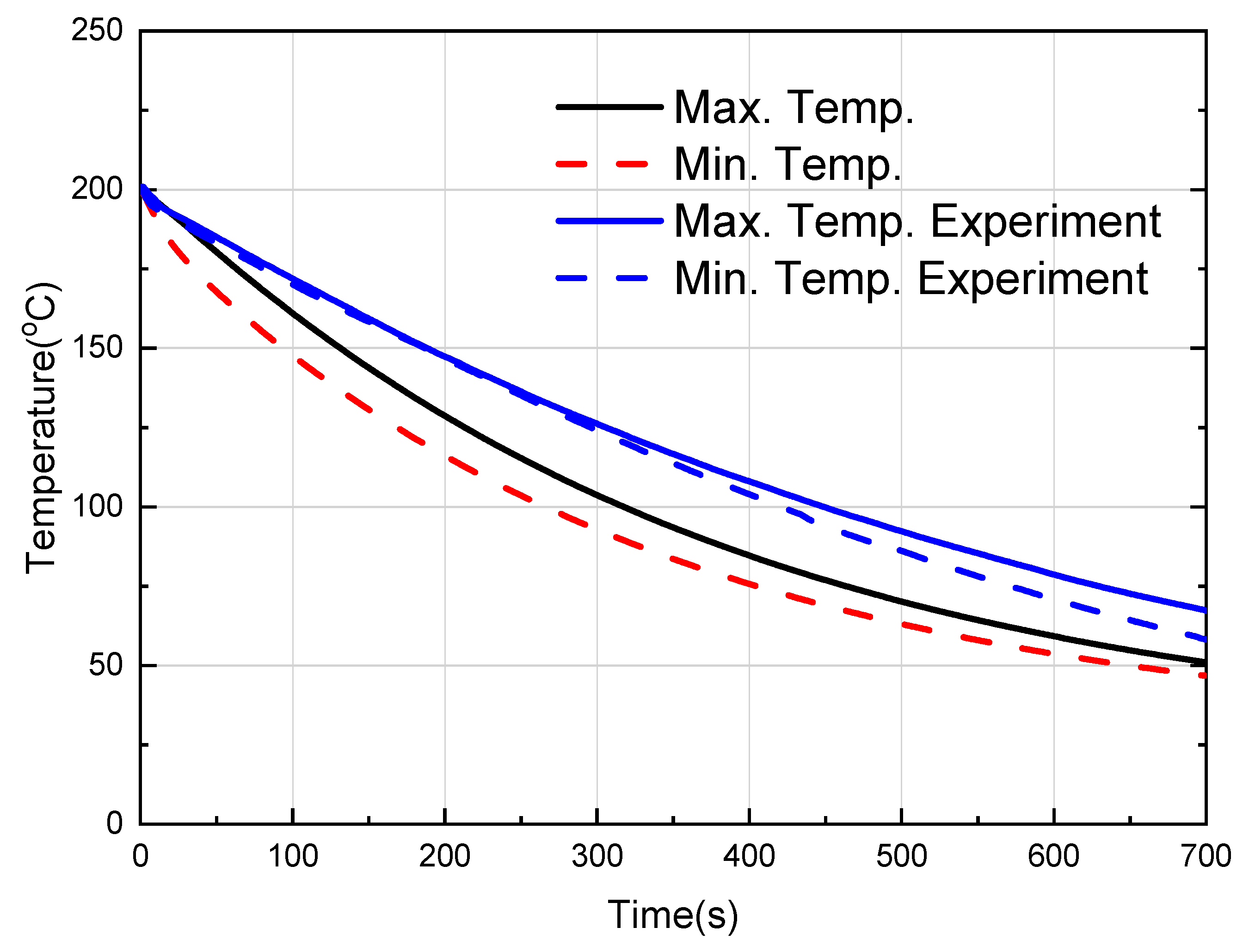
Figure 27 shows the experimental results of Yang [31] in which the cooling length is 3.0 cm and the heat pipes are cooled via water. Figure 28 shows the computational analysis results using the same cooling capacity along with the results of Yang [31]. In the computational analysis, when cooling is performed with air at 15 °C and a rate of 30 m/s, the temperature is greater than the experimental result. Rather than this being due to a problem in the calculation of the convective heat transfer coefficient, though heat transfer is achieved by the working fluid in the experiment, in the calculation, the heat pipe is modeled as a solid, and a general value for copper was applied for the selection of Cp. We compared the overall trends of the experimental and computational analyses to verify the validity and applicability of the numerical model.
4. Conclusions
To conduct the thermal design of a large-area hot plate for nanoimprint equipment, we selected the model to be studied and proposed a cooling model using both direct and indirect cooling methods with and without heat pipes. In addition, we created a small hot plate and performed experimental and computational analyses to confirm the validity of the proposed model. This study also analyzed problems that may occur in the stage prior to the large-area expansion of the hot plate. We fabricated the large-area hot plate from SUS (Steel Use Stainless) material and compared the results of the experiment and the computational analysis, and then developed a large-area hot plate and confirmed the superiority of the hot plate developed through practical application. The following conclusions were drawn from this study.
- (1)
- Based on the conceptual design, we developed a heating model with a controller to realize the unsteady temperature behavior. The PID algorithm was applied to the controller and its operability was evaluated by changing the values of Pgain, Igain, and Dgain. For cooling, hot plate cooling models incorporating and not incorporating heat pipes were developed in the same manner as the study model. When heat pipes are applied, indirect cooling is performed by cooling their ends.
- (2)
- A computational analysis was performed using a heating model including a controller that applies a stainless steel (STS304) material for the large-area expansion of the hot plate. The results demonstrated that the 2 cm ends of the cartridge heaters were not heated, and the thermal conductivity of the stainless steel was low. Thus, the maximum temperature difference at nine measurement points of the hot plate was 20 °C. For cooling, cooling holes were formed; when using nitrogen and water as the coolants and applying counter-flow, the temperature difference was 20 °C and 32.5 °C, respectively. These results confirmed issues with heating and cooling through conventional methods. To address the above problems, a new heating method was proposed applying heat pipes, and for the cooling method, an indirect cooling method was proposed in which the heat pipe ends are cooled.
- (3)
- When using a stainless steel (STS304) hot plate for large-area hot plate expansion, the heat pipes were inserted in the direction of the cartridge heaters to address the problems that may occur when expanding the hot plate into a large area. As a result, the heating rate was 40 °C/min and the temperature uniformity was less than 1% of the maximum working temperature of 200 °C. For cooling, when considering pressure and using air as the coolant for the ends, a cooling rate of 20 °C/min and thermal performance of less than 13.2 °C (less than 7%) based on the maximum temperature were obtained. These results were similar to the experimental results.
Author Contributions
Conceptualization, G.P.; methodology, C.L.; investigation, C.L.; data curation, G.P.; writing—original draft preparation, C.L.; writing—review and editing, C.L.
Funding
This research received no external funding.
Conflicts of Interest
The authors declare no conflict of interest.
References
- May, G.S.; Spanos, C.J. Fundamentals of Semiconductor Fabrication; John Wily & Sons Publishing: New York, NY, USA, 2003. [Google Scholar]
- Chou, S.Y.; Krauss, P.R.; Renstrom, P.J. Nanoimprint Lithography. J. Vac. Sci. Technol. 1996, 14, 129–4133. [Google Scholar] [CrossRef]
- Becker, H.; Heim, U. Hot Embossing as a Method for the Fabrication of Polymer High Aspect Ratio Structures. Sens. Actuators A Phys. 2000, 84, 130–135. [Google Scholar] [CrossRef]
- Lee, J.; Park, S.; Choi, K.; Kim, G. Nano-scale patterning using the roll typed UVnanoimprint lithography tool. Microelectron. Eng. 2008, 85, 861–865. [Google Scholar] [CrossRef]
- Ahn, S.H.; Guo, L.J. Large-area roll-to-roll and roll-to-plate Nanoimprint Lithography: A step toward high-throughput application of continuous nanoimprinting. ACS Nano. 2009, 3, 2304–2310. [Google Scholar] [CrossRef] [PubMed]
- Yoshikawa, H.; Taniguchi, J.; Tazaki, G.; Zento, T. Fabrication of high-aspect-ratio pattern via high throughput roll-to-roll ultraviolet nanoimprint lithography. Microelectron. Eng. 2013, 112, 273–277. [Google Scholar] [CrossRef]
- Hua, F.; Sun, Y.; Gaur, A.; Meitl, M.A.; Bilhaut, L.; Rotkina, L.; Wang, J.; Geil, P.; Shim, M.; Rogers, J.A.; et al. Polymer imprint lithography with molecular-scale resolution. Nano Lett. 2004, 4, 2467–2471. [Google Scholar] [CrossRef]
- Belligundu, S.; Shiakolas, P.S. Study on two-stage hot embossing microreplication: Silicon to polymer to polymer. J. Microlithogr. Microfabr. Microsyst. 2006, 5, 021103. [Google Scholar] [CrossRef]
- Jaszewski, R.W.; Schift, H.; Schnyder, B.; Schneuwly, A.; Gröning, P. Deposition of anti-adhesive ultra-thin teflon-like films and their interaction with polymers during hot embossing. Appl. Surf. Sci. 1999, 143, 301–308. [Google Scholar] [CrossRef]
- Chou, S.Y.; Krauss, P.R.; Renstrom, P.J. Imprint of sub-25 nm vias and trenches in polymers. Appl. Phy. Lett. 1995, 67, 3114. [Google Scholar] [CrossRef]
- Youn, S.W.; Ogiwara, M.; Goto, H.; Takahashi, M.; Maeda, R. Prototype development of a roller imprint system and its application to large area polymer replication for a microstructured optical device. J. Mater. Process. Technol. 2008, 202, 76–85. [Google Scholar] [CrossRef]
- Xia, Q.; Keimel, C.; Ge, H.; Yu, Z.; Wu, W.; Chou, S.Y. Ultrafast patterning of nanostructures in polymers using laser assisted nanoimprint lithography. Appl. Phy. Lett. 2003, 83, 4417–4419. [Google Scholar] [CrossRef] [Green Version]
- Hsu, Q.C.; Lin, Y.T.; Chou, D.C.; Wu, C.D. Study on Nanoimprint Formability Considering the Anti-adhesion Layer for (CH2) n Polymer by Molecular Dynamics Simulation. Curr. Nanosci. 2012, 8, 424–431. [Google Scholar] [CrossRef]
- Maury, P.; Escalante, M.; Reinhoudt, D.N.; Huskens, J. Directed assembly of nanoparticles onto polymer-imprinted or chemically patterned templates fabricated by nanoimprint lithography. Adv. Mater. 2005, 17, 2718–2723. [Google Scholar] [CrossRef]
- Retolaza, A.; Juarros, A.; Ramiro, J.; Merino, S. Thermal roll to roll nanoimprint lithography for micropillars fabrication on thermoplastics. Microelectron. Eng. 2018, 193, 54–61. [Google Scholar] [CrossRef]
- Andrews, D.L.; Lipson, R.H.; Nann, T.; Mohamed, K. Nanoimprint Lithography for Nanomanufacturing. In Comprehensive Nanoscience and Nanotechnology, 2nd ed.; Academic Press: Cambridge, MA, USA, 2019; pp. 357–386. [Google Scholar]
- Shan, X.; Liu, Y.C.; Lam, C. Studies of polymer deformation and recoveryin micro hot embossing. Microsyst. Technol. 2008, 14, 1055–1060. [Google Scholar] [CrossRef]
- Tan, H.; Gilbertson, A.; Chou, S.Y. Roller nanoimprint lithography. J. Vac. Sci. Technol. B Microelectron. Nanometer Struct. 1998, 16, 3926. [Google Scholar] [CrossRef]
- Striegel, A.; Schneider, M.; Schneider, N.; Benkel, C.; Worgull, M. Seamless tool fabrication for Roll-to-Roll microreplication. Microelectron. Eng. 2018, 194, 8–14. [Google Scholar] [CrossRef]
- Ahn, S.; Cha, J.; Myung, H.; Kim, S.M.; Kang, S. Continuous ultraviolet roll nanoimprinting process for replicating large-scale nano-and micropatterns. Appl. Phys. Lett. 2006, 89, 12–15. [Google Scholar] [CrossRef]
- Moro, M.; Taniguchi, J.; Hiwasa, S. Fabrication of antireflection structure film by roll-to-roll ultraviolet nanoimprint lithography. J. Vac. Sci. Technol. B Nanotechnol. Microelectron. Mater. Process. Meas. Phenom. 2014, 32, 06FG09. [Google Scholar] [CrossRef]
- Chou, S.Y.; Keimel, C.; Gu, J. Ultrafast and direct imprint of nanostructures in silicon. Nature 2002, 417, 835–837. [Google Scholar] [CrossRef]
- Cui, B.; Keimel, C.; Chou, S.Y. Ultrafast direct imprinting of nanostructures in metals by pulsed laser melting. Nanotechnology 2010, 21, 045303. [Google Scholar] [CrossRef] [PubMed]
- Moore, S.; Gomez, J.; Lek, D.; You, B.H.; Kim, N.; Song, I.H. Experimental study of polymer microlens fabrication using partial-filling hot embossing technique. Microelectron. Eng. 2016, 162, 57–62. [Google Scholar] [CrossRef]
- Pang, S.W.; Tamamura, T.; Nakao, M.; Ozawa, A.; Masuda, H. Direct Nano-Printing on Al Substrate Using a SiC Mold. J. Vac. Sci. Technol. 1998, 16, 1145–1149. [Google Scholar] [CrossRef]
- Hirai, Y.; Fujiwara, M.; Okuno, T.; Tanaka, Y.; Endo, M.; Irie, S.; Nakagawa, K.; Sasago, M. Study of the Resist Deformation in Nanoimprint Lithography. J. Vac. Sci. Technol. 2001, 19, 2811–2815. [Google Scholar] [CrossRef]
- Beck, M.; Graczyk, M.; Maximov, I.; Sarwe, E.L.; Ling, T.G.I.; Keil, M.; Montelius, L. Motelius, Improving Stam4ps or 10 nm Level Wafer Scale Nanoimprint Lithography. Microelectron. Eng. 2002, 61, 441–448. [Google Scholar] [CrossRef]
- Khang, D.Y.; Kang, H.; Kim, T.I.; Lee, H.H. Low-Pressure Nanoimprint Lithography. Nano Lett. 2004, 4, 633–637. [Google Scholar] [CrossRef]
- Kwak, H.S.; Park, G.J.; Son, B.C.; Lee, J.J.; Park, H.C. Design of a Hot plate with Rapid Cooling Capability or Thermal Nanoimprint Lithography. In Proceedings of the SICE-ICASE International Joint Conference, Busan, Korea, 18–21 October 2006; pp. 4897–4901. [Google Scholar]
- Park, G.J.; Kwak, H.S.; Shin, D.W.; Lee, J.J. Numerical Simulation of Thermal Control of a Hot Plate for Thermal Nanoimprint Lithography Machines. In Proceedings of the 3rd International Conference on Heating Cooling Technol, Seoul, Korea, 4 March 2007; pp. 321–327. [Google Scholar]
- Yang, J.H. An Experimental Study on the Thermal Performance of a Hot Plate for Thermal Nanoimprint Lithography. Master’s Thesis, Kumoh National Institute of Technology, Gumi, Korea, 2008. [Google Scholar]
- Faghri, A. Heatpipe Science and Technology; Taylor & Francis Press: Abingdon, UK, 1995. [Google Scholar]
- Wallin, P. Heat Pipe: Selection of Working Fluid; Heat and Mass Trasfer Project Report; MVK160: Lund, Sweden, 7 May 2012; pp. 1–7. [Google Scholar]
- Cengel, Y.A. Heat and Mass Transfer; McGraw-Hill Press: New York, NY, USA, 2012; pp. 521–527. [Google Scholar]
- Yakhot, V.; Orszag, S.A.; Thangam, S.; Gatski, T.B.; Speziale, C.G. Development of turbulence models for shear flows by a double expansion technique. Phys. Fluids A 1992, 4, 1510–1520. [Google Scholar] [CrossRef] [Green Version]
Figure 1.
Schematic diagram of the experimental setup for the heating test with a small hot plate.

Figure 2.
Temperature controller system diagram for two cartridge heaters.

Figure 3.
Schematic diagram of the hot plate: (a) Top view and front view, (b) sub zone, (c) mesh structure of simulation model.
Figure 3.
Schematic diagram of the hot plate: (a) Top view and front view, (b) sub zone, (c) mesh structure of simulation model.


Figure 4.
Effect on Igain on time-dependent evolution of temperature at the center of the hot plate made of aluminum (Igain = 0, Dgain =0).
Figure 4.
Effect on Igain on time-dependent evolution of temperature at the center of the hot plate made of aluminum (Igain = 0, Dgain =0).

Figure 5.
Effect on Igain on the rate of heat generation of the heater.

Figure 6.
Effect on Igain on time-dependent evolution of the temperature at the center of the hot plate made of aluminum (Pgain = 5 A, Dgain = 0).
Figure 6.
Effect on Igain on time-dependent evolution of the temperature at the center of the hot plate made of aluminum (Pgain = 5 A, Dgain = 0).

Figure 7.
Effect of Igain on the rate of heat generation of the heater.

Figure 8.
Effects of Dgain on the time-dependent evolution of temperature at the center of the hot plate made of aluminum. The small graph in the lower right corner shows the steady-state results. Pgain = 2 A, Igain = 0.
Figure 8.
Effects of Dgain on the time-dependent evolution of temperature at the center of the hot plate made of aluminum. The small graph in the lower right corner shows the steady-state results. Pgain = 2 A, Igain = 0.

Figure 9.
Effect on Igain on the rate of heat generation of the heater.

Figure 10.
Time-dependent evolution of the temperature at the center of the hot plate made of aluminum using PID controlled heater.
Figure 10.
Time-dependent evolution of the temperature at the center of the hot plate made of aluminum using PID controlled heater.

Figure 11.
Effect on control parameters on the time-dependent temperature evolution at the center on the upper surface of the sub zone. (a) Proportional gain effect; (b) integral gain effect with Pgain = 3 A.
Figure 11.
Effect on control parameters on the time-dependent temperature evolution at the center on the upper surface of the sub zone. (a) Proportional gain effect; (b) integral gain effect with Pgain = 3 A.

Figure 12.
Time-dependent temperature evolution at the six points on the upper surface of the large-area hot plate without heat-pipe calculated by CFD.
Figure 12.
Time-dependent temperature evolution at the six points on the upper surface of the large-area hot plate without heat-pipe calculated by CFD.

Figure 13.
Time-dependent variation of the temperature difference at the six points on the upper surface of the hot plate calculated by CFD.
Figure 13.
Time-dependent variation of the temperature difference at the six points on the upper surface of the hot plate calculated by CFD.

Figure 14.
Time-dependent temperature evolution at the six points on the upper surface of the large-area hot plate with heat pipes.
Figure 14.
Time-dependent temperature evolution at the six points on the upper surface of the large-area hot plate with heat pipes.

Figure 15.
Temperature [K] distribution on the upper surface of the hot plate.


Figure 16.
Temperature variation at the surface of the hot plate after turning on counter-directional nitrogen cooling flows for a large-area hot plate.
Figure 16.
Temperature variation at the surface of the hot plate after turning on counter-directional nitrogen cooling flows for a large-area hot plate.

Figure 17.
Variation of maximum temperature difference on the surface of the hot plate after turning on counter-directional nitrogen cooling for a large-area hot plate.
Figure 17.
Variation of maximum temperature difference on the surface of the hot plate after turning on counter-directional nitrogen cooling for a large-area hot plate.

Figure 18.
Temperature variation at the surface of the hot plate after turning on counter-directional water-cooling flows for a large-area hot plate.
Figure 18.
Temperature variation at the surface of the hot plate after turning on counter-directional water-cooling flows for a large-area hot plate.

Figure 19.
Variation of maximum temperature difference on the surface of the hot plate after turning on counter-directional water cooling for a large-area hot plate.
Figure 19.
Variation of maximum temperature difference on the surface of the hot plate after turning on counter-directional water cooling for a large-area hot plate.

Figure 20.
Time-dependent variation of the temperature at the six points on the upper surface of the hot plate by direct cooling using heat pipes.
Figure 20.
Time-dependent variation of the temperature at the six points on the upper surface of the hot plate by direct cooling using heat pipes.

Figure 21.
Time-dependent variation of the temperature difference at the six points on the upper surface of hot plate by direct cooling using heat pipes.
Figure 21.
Time-dependent variation of the temperature difference at the six points on the upper surface of hot plate by direct cooling using heat pipes.

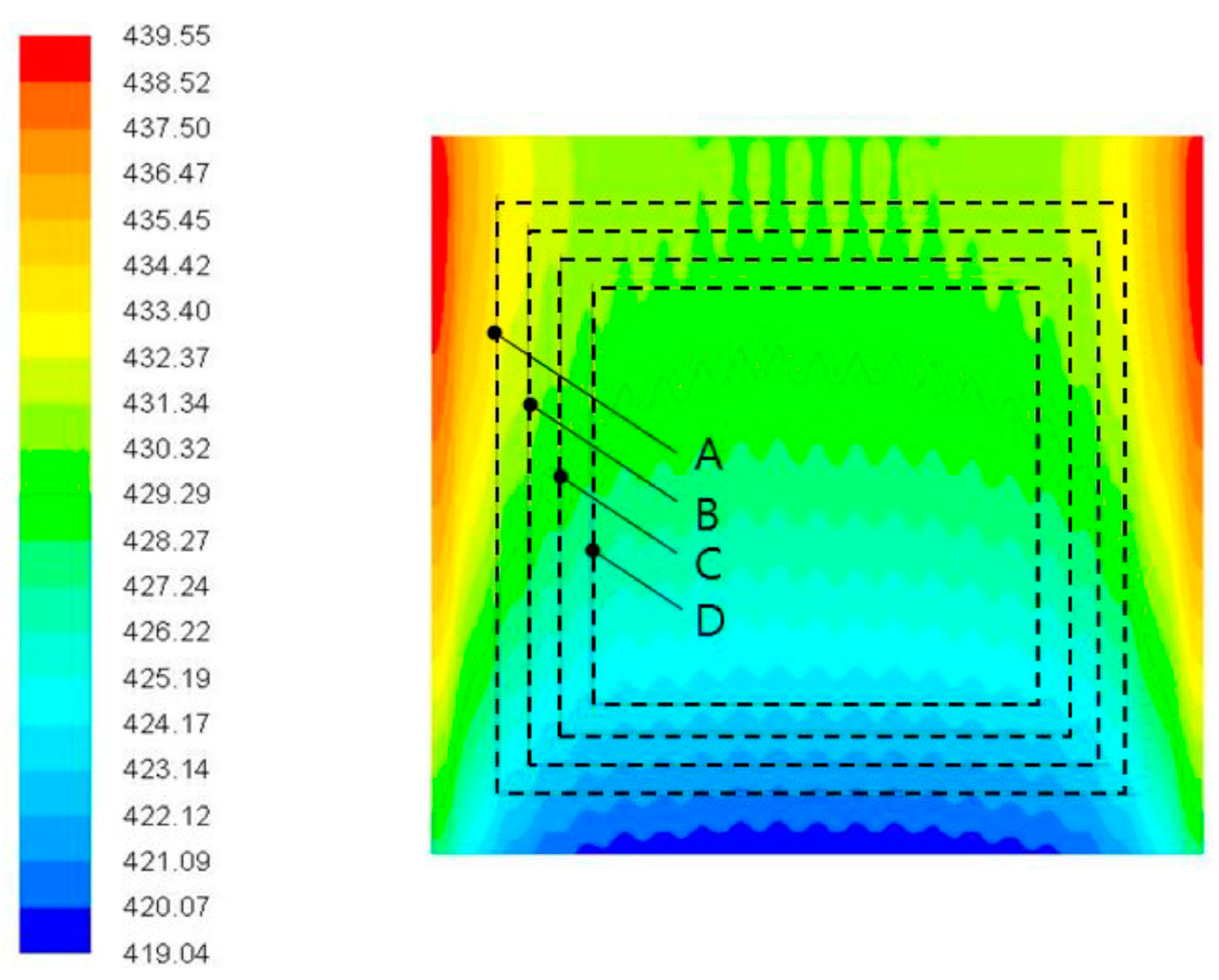
Figure 22.
Working area possible after 100 s by direct cooling using heat pipes. (Temperature and velocity of coolant are 15 °C and 30 m/s).
Figure 22.
Working area possible after 100 s by direct cooling using heat pipes. (Temperature and velocity of coolant are 15 °C and 30 m/s).

| Area | Temperature difference Max. Temp.–Min. Temp. | Working area (cm2) |
| A | 13.3 | 200 × 200 |
| B | 11.0 | 190 × 190 |
| C | 9.0 | 180 × 180 |
| D | 1.0 | 170 × 170 |
Figure 23.
Working area possible after 700 s by direct cooling using heat pipes. (Temperature and velocity of coolant are 15 °C and 30 m/s).
Figure 23.
Working area possible after 700 s by direct cooling using heat pipes. (Temperature and velocity of coolant are 15 °C and 30 m/s).

| Area | Temperature difference Max. Temp.–Min. Temp. | Working area (cm2) |
| A | 4.1 | 200 × 200 |
| B | 3.5 | 190 × 190 |
| C | 2.9 | 180 × 180 |
| D | 1.3 | 170 × 170 |
Figure 24.
Results of the heating experiment [31], showing temporal evolution of temperature at the surface of the hot plate without heat pipes.
Figure 24.
Results of the heating experiment [31], showing temporal evolution of temperature at the surface of the hot plate without heat pipes.

Figure 25.
Comparison of experiments [31] and CFD result for time-dependent temperature evolution at the six points on the upper surface of the large-area hot plate without heat pipes.
Figure 25.
Comparison of experiments [31] and CFD result for time-dependent temperature evolution at the six points on the upper surface of the large-area hot plate without heat pipes.

Figure 26.
Comparison of experiments [31] and CFD results for time-dependent temperature evolution at the six points on the upper surface of the large-area hot plate with heat pipes.
Figure 26.
Comparison of experiments [31] and CFD results for time-dependent temperature evolution at the six points on the upper surface of the large-area hot plate with heat pipes.

Figure 27.
Results of cooling experiments [31] by using water injection (the length of condenser section is 30 mm).
Figure 27.
Results of cooling experiments [31] by using water injection (the length of condenser section is 30 mm).

Figure 28.
Comparison of experiment [31] and CFD result for time-dependent variation of the maximum temperature and that of the minimum temperature at the six points on the upper surface of the large area hot plate by indirect cooling using heat pipes.
Figure 28.
Comparison of experiment [31] and CFD result for time-dependent variation of the maximum temperature and that of the minimum temperature at the six points on the upper surface of the large area hot plate by indirect cooling using heat pipes.


| NIL Method | Process Details | Mold/Substrate | Resist Materials |
|---|---|---|---|
| Thermal NIL [19,20] | Thermal annealing of polymers at temperatures up to 50 °C above the glass transition temperature. | High hardness molds (Young’s modulus should be higher than that of resist): silicon, glasses, quartz, nickel, ceramics, Al oxide Note: thermal expansion coefficient of mold and substrate should match | Only thermoplastic polymers: polystyrene (PS), poly(methyl-methacrylate) (PMMA), polycarbonate (PC), polyethylene terephthalate (PET), siloxane copolymers (PDMS-b-PS, PDMS-g-PMMA), specified spin-on polymers |
| UV NIL at room temperature [4,5,6,21,22] | UV, EUV exposure | UV-transparent materials: quartz glass; soft stamps are more common for UV NIL: polydimethylsiloxane (PDMS), polyvinyl chloride (PVC), PMMA | Low viscosity UV-sensitive materials, ideally with low volume shrinkage after polymerization—usually liquid functionalized monomers or oligomers, CARs (Chemical amplified resists) |
| UV NIL + thermal annealing [23,24] | Simultaneous UV exposure and substrate heating | UV-transparent materials | UV-curable polymers with better surface coverage and lower imprint temperatures as for T-NIL can be used |
Table 2.
Specifications of instruments.
| Items | Model | Specifications | Remarks |
|---|---|---|---|
| Data acquisition system | Agilent 34970A | Two 8-bit digital I/O ports, 26-bit Event Counter, Two 16-bit Analog outputs | Data logger of temperature |
| Power supply | WYG 1C 20Z4 | 90~240 VAC | 8.3 ± 1 ms (response time) |
| Feedback controller | TZN4S | PID (Proportional integral derivative) control | Temperature controller |
| Temperature sensor | K-type thermocouple | 2.0 mm diameter | ±1.5 °C |
Table 3.
Specification of large-area hot plate.
| Mark | Length [mm] |
|---|---|
| G | 20 |
| L | 240 |
| Lhp | 340 |
| S | 12 |
| Dhp | 6 |
| Dch | 6 |
| H | 20 |
| Hth | 8 |
© 2019 by the authors. Licensee MDPI, Basel, Switzerland. This article is an open access article distributed under the terms and conditions of the Creative Commons Attribution (CC BY) license (http://creativecommons.org/licenses/by/4.0/).
Share and Cite
MDPI and ACS Style
Park, G.; Lee, C. Experimental and Numerical Study on the Characteristics of the Thermal Design of a Large-Area Hot Plate for Nanoimprint Equipment. Sustainability 2019, 11, 4795. https://0-doi-org.brum.beds.ac.uk/10.3390/su11174795
AMA Style
Park G, Lee C. Experimental and Numerical Study on the Characteristics of the Thermal Design of a Large-Area Hot Plate for Nanoimprint Equipment. Sustainability. 2019; 11(17):4795. https://0-doi-org.brum.beds.ac.uk/10.3390/su11174795
Chicago/Turabian StylePark, Gyujin, and Changhee Lee. 2019. "Experimental and Numerical Study on the Characteristics of the Thermal Design of a Large-Area Hot Plate for Nanoimprint Equipment" Sustainability 11, no. 17: 4795. https://0-doi-org.brum.beds.ac.uk/10.3390/su11174795
Note that from the first issue of 2016, this journal uses article numbers instead of page numbers. See further details here.