Factors Influencing Matching of Ride-Hailing Service Using Machine Learning Method

1
Department of Urban Engineering, Hanbat National University, Daejeon 34158, Korea
2
Future Strategy Research Center, Land & Housing Institute, Daejeon 34047, Korea
3
DataWiz Ltd., Mokwon University, Daejeon 35349, Korea
4
Center of Infrastructure Asset Management, Hanbat National University, Daejeon 34158, Korea
*
Author to whom correspondence should be addressed.
Sustainability 2019, 11(20), 5615; https://0-doi-org.brum.beds.ac.uk/10.3390/su11205615
Submission received: 19 August 2019
/
Revised: 1 October 2019
/
Accepted: 8 October 2019
/
Published: 12 October 2019
(This article belongs to the Special Issue Sustainability in 2nd IT Revolution with Dynamic Open Innovation)
Abstract
:It is common to call a taxi by taxi-apps in Korea and it was believed that an app-taxi service would provide customers with more convenience. However, customers’ requests can often be denied, as taxi drivers can decide whether to take calls from customers or not. Therefore, studies on factors that determine whether taxi drivers refuse or accept calls from customers are needed. This study investigated why taxi drivers might refuse calls from customers and factors that influence the success of matching within the service. This study used origin-destination data in Seoul and Daejeon obtained from T-map Taxis, which was analyzed via a decision tree using machine learning. Cross-validation was also performed. Results showed that distance, socio-economic features, and land uses affected matching success rate. Furthermore, distance was the most important factor in both Seoul and Daejeon. The matching success rate in Seoul was lowest for trips shorter than the average at midnight. In Daejeon, the rate was lowest when the calls were made for trips either shorter or longer than the average distance. This study showed that the matching success for ride-hailing services can be differentiated particularly by the distance of the requested trip depending on the size of the city.
1. Introduction
With the rapidly growing use of smartphones, customers can make purchases exclusively using apps on a smartphone. Online-to-offline (O2O) service is a business model for making potential customers buy goods in physical stores through online channels. The expansion of O2O services has stimulated the growth of ride-hailing services in the transportation sector over the world. For example, the ride-hailing service in China expanded to various transportation forms and is getting more influential in personal mobility [1]. Ride-hailing is different from ride-sharing. Ride-hailing is the service where riders hire a personal driver who takes them to the exact destination requested. By contrast, ride-sharing is the service where a vehicle is shared with other riders who have a different destination to each other; ride-sharing is not a personal service.
In Korea, ride-hailing services and taxi-apps offered by companies such as Kakao Taxi and T-map Taxi are becoming increasingly popular. However, despite the belief that an app-taxi service would provide customers with more convenience, there have been complaints about the service offered to customers. Customers’ requests can often be denied, as taxi drivers can decide whether to take calls from customers or not after checking their origin and the destination requested.
Although it may not be possible to have a perfect balance between the requirements of taxi drivers and demands of customers, it may be possible to meet the demand of customers using another on-demand service, such as ride-sharing. However, there have been huge protests and resistance from taxi drivers in Korea against ride-sharing services. Therefore, at this time of day, such a service being introduced still requires careful consideration. Therefore, studies on the reasons for the difference between the requirements of taxi drivers and the demands of customers, as well as factors that determine whether taxi drivers refuse or accept calls from customers are needed.
Several studies have been conducted on the use of shared transportation services and they focused on social benefits such as reduction of traffic congestion [2] and greenhouse gas emissions [3]. However, this study focuses on reviewing studies on ride-hailing.
Liao [4] developed and implemented an automatic vehicle location and dispatch system for three taxi companies in Singapore, based on the Global Positioning System (GPS). The system can increase the performance of taxi service management. Customer satisfaction in terms of the performance of the system was high, and it was also expected that the matching rate between passengers and taxi drivers would be improved.
Seow et al. [5] investigated a new dispatch system for taxis in Singapore using a simulation technique and achieved high customer satisfaction. They proposed dispatching multiple taxis to the same number of customers in the same area, and the results show that the waiting time of taxi users reduced by up to 33.1% compared with a previous dispatch system, whereas the idling time of taxis reduced by 26.3%.
Tao [6] carried out a pilot study with intelligent transportation system (ITS) technology in Taipei, Taiwan to examine the matching success rate of a taxi sharing system. The author conducted a survey of users who utilized the service. The results show that approximately 70% of the respondents were women, whereas 90% of them were captive riders in their 20s or 40s. The system also yielded 60% success rate in matching between taxis and users. The results also showed that a higher matching success rate was achieved when more users used public transportation for their trips; most of the respondents were satisfied with the service, but also indicated that the interface of the website for the service was not convenient.
Wallsten [7] used detailed data sets from the New York City Taxi and Limousine Commission documenting more than 1 billion cab uses, complaints about taxis in New York and Chicago, and information provided by Google Trends. He analyzed the competitive effects on the vehicle sharing service of Uber, one of the largest ride-hailing companies in the world. Uber’s popularity was linked to the decline of customer complaints about the taxi service in New York, whereas its growth in Chicago was linked to the decline of certain types of complaints about taxis, including credit card machine breakdown, heating, disrespect, and mobile phone calls by taxi drivers.
Keong [8] analyzed a survey of 305 Malaysian taxi drivers on factors affecting taxi drivers’ use of mobile taxi applications. He found that drivers’ use of such applications was affected by their relative advantages, complexity, drivers’ knowledge, and coercive, mimetic and normative pressures.
Saadi et al. [9] used data from a major Chinese ride-hailing service provider, DiDi Chuxing, and analyzed the temporal and spatial estimation of demand using several machine learning techniques to characterize and predict the short-term demand for ride-hailing services. The machine learning techniques used include decision tree, bagged decision tree, random forest, the gradient boosted decision tree, and an artificial neural network for regression. The gradient boosted decision tree yielded the lowest RMSE (16.41), followed by the artificial neural network (20.09), the random forest (23.50), the begged decision tree (24.29), and the decision tree (33.55). The results show that demand prediction using the gradient boosted decision tree can meet the driver’s requirements more efficiently.
Most studies on app-taxi services focused on usage of services, customer satisfaction, and the success rate of matching between taxi drivers and customers. Furthermore, factor analysis with customer survey was mostly used for identifying the main factors that influence the use of app-taxis and customers’ satisfaction. However, machine learning was scarcely used in previous studies to identify factors influencing the success rate of matching between customers and taxi drivers as well as cross-city comparison approach.
Thus, this study aims to identify factors influencing matching of ride-hailing services from taxi drivers’ point of view using machine learning. A cross-city comparison is also performed to determine the influence of the sizes of cities. In addition, cross validation is carried out to minimize overfitting or selection bias based on the study in [10]. The findings of this study provide insights on how the gap between customers and taxi drivers can be bridged. Furthermore, the study also provides directions on how to improve ride-hailing services in mega cities and medium-sized cities, as well as the features of app-taxi services in such cities.
2. Methodology
2.1. Machine Learning and Decision Tree
Machine learning is used to construct a decision tree to determine the factors influencing matching and to build models. As one of the machine learning algorithms, decision trees chart several decision-making rules and classify or predict a few small groups concerned. They have several sub-models based on the splitting criteria and stopping rules to prevent further data splitting, including chi-squared automatic interaction detection (CHAID), classification and regression trees (CART), C5.0 (successor of ID4), C4.5 (successor of ID3), and Iterative Dichotomiser 3 (ID3). The basic structure of a decision tree is shown in Figure 1 [11].
This model can be easily understood owing to its tree-like structure. In addition, it is a non-parametric method, which does not require the assumption of linearity, normality, or homoscedasticity. Therefore, it is not sensitive to outliers and is superior to existing statistical models in terms of prediction [12].
In this study, a CART algorithm was used to form a regression tree as the dependent variables were continuous. The CART algorithm performs binary split and has different splitting criteria. It also forms a classification tree with discrete dependent variables and a regression tree with continuous dependent variables. The classification tree uses the Gini index as a splitting criterion, as given in the following equation. The Gini index measures the impurity or diversity in each node. It determines the probability of two elements randomly extracted from the total elements that belong to different groups.
where is the Gini index, is the number of categories of the target variables, is the probability that an object in each node belongs to the jth category of the target variable, is the number of observations included in parent node, and is the number of observations in the jth category of the target variable.
A classification tree chooses the dependent variable that reduces the Gini index to the greatest degree and achieves optimal splitting of the variable as child nodes; the decrease in the Gini index is estimated, as given in the following equation. This is to form child nodes so that the impurity is at the lowest level in the case of classification into child nodes [13].
where is the decrease in the Gini index, is the Gini index of the parent node, is the number of observations in the parent node, are the number of observations in the left child node and right child node, respectively, and are the Gini indices of the left child node and the right child node, respectively.
This study used scikit-learn, which is one of the libraries for the Python programming language. Scikit-learn can favorably provide a user-friendly, efficient, and productive interface when implementing an algorithm. It is available in several distribution versions of the Python language such as Anaconda, Enthought Canopy, and Python (x, y). Anaconda is particularly useful for analyzing mass data and performing predictive analysis [14,15]. Therefore, this study used Anaconda for decision tree analysis to form a regression tree.
2.2. Cross-Validation and Model Optimization
Machine learning algorithms are better at predicting explanatory power and building efficient models than conventional methods. However, machine learning exhibits the problem of overfitting. CART algorithm also has an overfitting problem as it is one of the machine learning algorithms. Therefore, a cross-validation technique was used to generalize the models without overfitting. Cross-validation is a technique that optimizes the balance between complexity and classification errors of decision trees. Although a tree grows and has more terminal nodes, the errors decrease; however, this also means that the model performs poorly with new data. Therefore, cross-validated was carried out in this study using a cost-complexity function [16,17].
where is the misclassification error of tree, T, is the complexity measure, which depends on , is the total sum of terminal nodes in the tree, and is a parameter.
Data for machine learning are divided into two data sets: training data and test data. Some of the data is used as the training data to form a tree. The parameter is a regularization parameter, which appears according to the orders of inputting the observations for a training phase of a model. The remaining data becomes the test data for a test phase. These steps were randomly iterated.
Exhaustive search, also known as brute-force or generate and test, was used to select two parameters, namely the maximum depth and minimum sample size of leaf nodes for the optimized tree models [18]. The method calculates all possible number of cases in the combinations of the depth of a tree between 1 and 10 and the minimum sample size of leaf nodes, and then selects parameters from the best fit case [19]. After performing this step, the maximum tree depth and the minimum sample size of leaf nodes for Seoul were selected as 4 and 1, respectively, whereas those for Daejeon were selected as 4 and 9, respectively.
3. Analysis of Features of App-Taxi Matching
In this study, the daily average trip distances of cities and counties in Korea, denoted as Si and Gun, respectively, were analyzed. Seventy-two cities and counties were divided into five regions; then, the daily average trip distances were calculated for each region according to trip purposes and trip means. This approach was used to compare the effects of app-taxi matching based on the characteristics of cities, such as population and distance. Results show that the capital region, including Seoul, had the longest distances of 9.5 km and 8.8 km for trip purposes and trip means, respectively, whereas the Daejeon region had the shortest distances of 5.8 km and 5.9 km, respectively, as shown in Figure 2. The results for Seoul and Daejeon, representing the longest and shortest trip distances, respectively were compared.
The population of Seoul in 2019 was estimated at 9.7 million and the city of Seoul covers a surface area of 605.2 km2. The population density is the city is 16,136 people/km2. On the other hand, Daejeon has a population of 1.5 million in 2019 and the city area is 539.4 km2. The population density is the city is 2785 people/km2. The geographical sizes of the cities are similar, but the population and population density of Seoul are over six times larger than the population and population density of Daejeon.
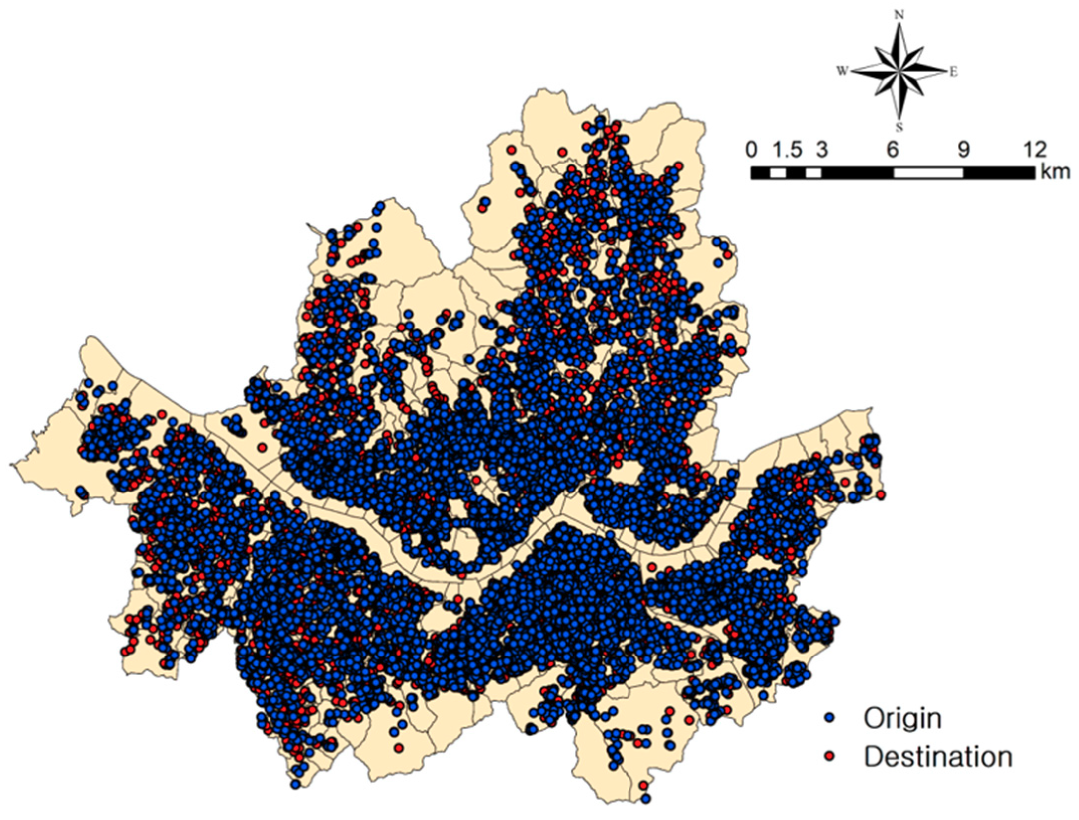
In this study, Origin-Destination (OD) data on successful and unsuccessful (failed) matchings decided by taxi drivers of T-map taxi service in Seoul and Daejeon Metropolitan City in April 2017 (Table 1) was used. The data included the date and time of customers’ calls, matching successes or failures, and categorized reasons for these matching failures as well as the origins and destinations (ODs). The distribution of ODs of the target cities is shown in Figure 3 and Figure 4.
According to data provided by T-map, there were 30,990 cases in Seoul and 4294 cases in Daejeon. The study focuses on identifying what makes taxi-drivers refuse calls from customers. Thus, of the cases, 21,785 cases in Seoul (70.3%) and 3112 cases in Daejeon (72.5%) were used in this study to examine whether taxi drivers accept or decline a call.
Matching success was set as the dependent variable (1 for success and 0 for fail) to analyze factors influencing matching success. Various features of information related to the origins and destinations recorded in the ODs were set as independent variables, namely socio-economic indicators, land uses, station influence area, time, weather, weekday or weekend, etc.
The socio-economic variables include population density, business density, and employee density of the origins and destinations. They were obtained from the Open Data portal for Seoul and National Statistics for Daejeon. The land use data of the ODs were extracted from GIS data in the National Spatial Data Infrastructure Portal. Influence of subway stations was estimated and used as an independent variable. Sta-Inf was defined as an area within a radius of 400 m around a subway station. Data of stations was obtained from the website of the Korea Transport Data Base (KTDB). Weather data was sourced from daily weather information recorded by the Korea Meteorological Administration. Details of the variables are presented in Table 2.
4. Results of Machine Learning
This study used supervised learning, which predicts a dependent (target) variable based on input data. The dependent variable was predicted based on separated input data: training set and test set. We analyzed 75% of the data for the training set and 25% for the test set.
Table 3 shows the results of empirical analysis using machine learning models. In terms of the results obtained before performing cross-validation, the explanation powers (R2) of the training set and test set were respectively 0.770 and 0.723 in Seoul and 0.757 and 0.766 in Daejeon. The decision tree derived the important ranks of the dependent variables as it employs the non-parametric method. The results show that distance was the most important variable in both Seoul and Daejeon.
However, the R2s of the results for the training set and test set in Seoul increased to 0.780 and 0.772, respectively after performing cross-validation. There were also significant increases of 0.836 and 0.834 for the training set and test set in Daejeon, respectively. Thus, cross-validation clearly increased the explanation powers in both cities.
Cross-validation clearly distinguished the important and unimportant variables; no value at Importance for unimportant variables. Five variables were identified as important for Seoul, namely Distance X(6), Midnight X(8), Peak time X(9), D_Employee density X(5), and O_Employee density X(2) in order of importance, whereas eight variables were identified as important for Daejeon, namely Distance, Peak time, Weekend, Cloudy, O_Business density, O_Population density, D_Population density, and O_ Employee density.
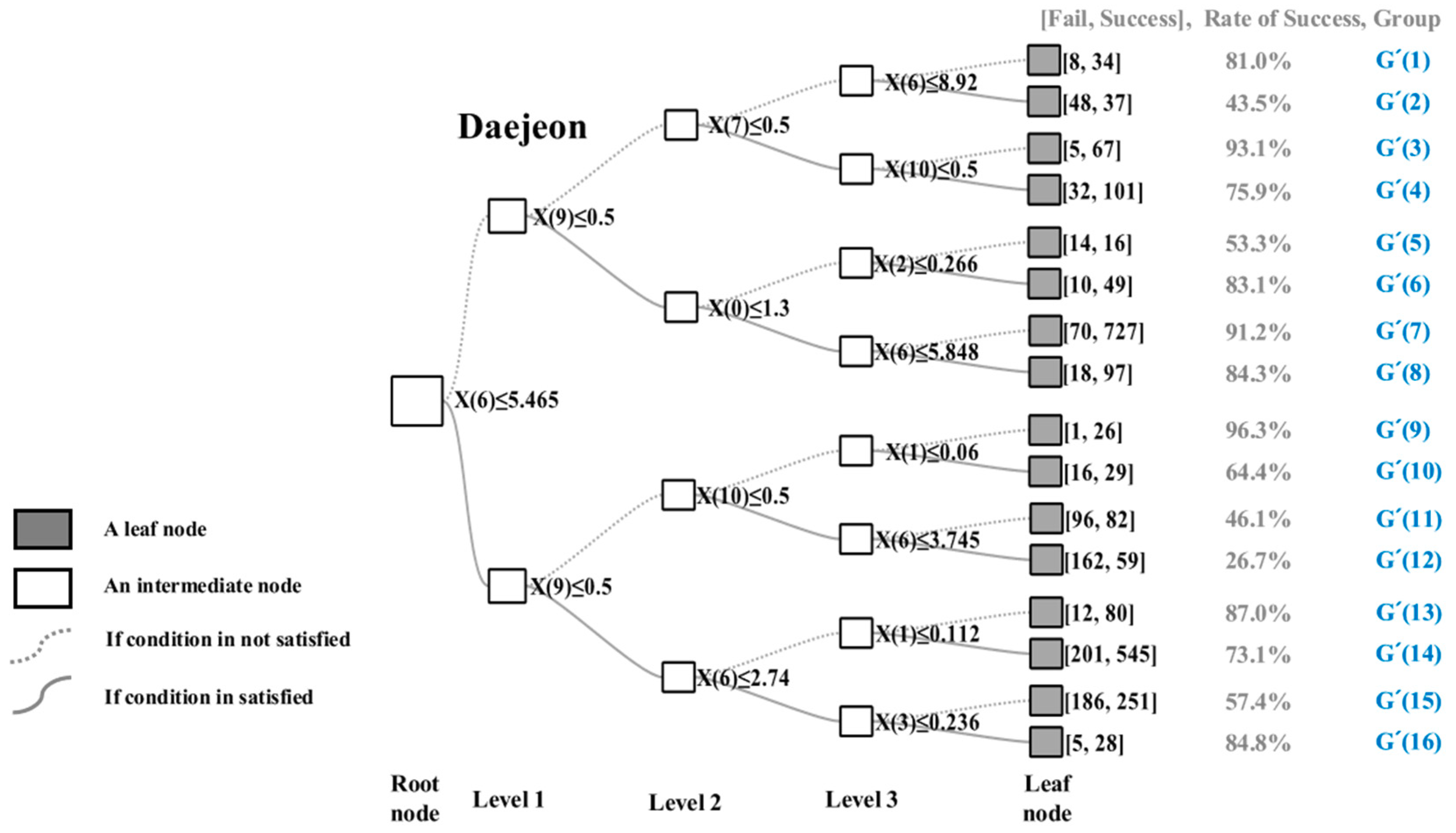
The results shown in Figure 5 and Figure 6 were obtained from the decision tree. The tree consists of 18 leaf nodes in grey squares, 15 internal nodes in white squares, and 1 root node in a slightly larger white square in the middle of the left side. The root node is the start of the tree and allows us to track down the classifications of data. The equations next to the white square nodes are the conditions for splitting the samples, and X(n)s are the dependent variables in Table 3. The solid lines in the figure indicates that the condition for splitting at each variable was met, whereas the dashed lines indicate that the condition was not met [20]. For example, in Figure 5, the root node had X(6) ≤ 8.155 with a dashed line in the upper side and a solid line in the lower side. This indicates that Distance X(6) was the dependent variable and the samples were split at a distance of 8.155 km (splitting condition). The samples that were at a distance of 8.155 km or less belonged to the lower side, whereas the other samples belonged to the upper side. In terms of the values next to the leaf nodes, the first values are the counts of the failed cases of matching, whereas the second values are those of the success cases. Each leaf node also indicates the success rate of matching on the right side. As previously explained, the decision tree shows a clear structure of the model.
In the results for Seoul (Figure 5), most of the leaf nodes with over 50% matching success rate were in the upper half of the decision tree diagram. Only 2 out of 8 leaf nodes in the upper half side had less than 50% matching success rate, whereas only 1 out of 8 leaf nodes in the lower half side had more than 50% matching success rate. This shows that X(6) Distance, which is the variable used for the first branch, is the most important factor and the matching success rates were clearly and mostly identified. When the trip distance for a certain call is less than 8.155 km, the call has a high possibility of being refused by a taxi driver. Apart from distance (X(6)), midnight (X(8)) and peak-time (X(9)) were also important factors.
Two patterns for low-matching success rates were particularly identical in Seoul (Figure 6). Although the trip distance for calls in Group 4 (Pattern 1) were long (over 8.155 km), the calls were made at night and the destinations had a relatively low employee density rate (X(5) ≤ 1.723). Therefore, the matching success rate was low. The calls in Groups 9 and 10 were for relatively short-distance trips (Pattern 2); short-distance trips tended to be frequently refused. However, Pattern 2 had even lower matching success rates as the calls were made at night and the employee density rate at the origins was high. Patterns 1 and 2 were both for trips at night; however, there were a few differences. Pattern 1 was for long-distance trips with a low possibility of taking another passenger at the destinations, whereas Pattern 2 was for short-distance trips with high demands at the origins. This means that taxi drivers can easily find passengers at the origins for Pattern 2. The results in Seoul show that taxi drivers clearly made selective choices for calls based on the trip distance and demand for taxis, especially the demand at origins.
In the results for Daejeon (Figure 7), there were only three leaf nodes with less than 50% matching success rate. This indicates that taxi drivers in Daejeon tended to refuse a call less than drivers in Seoul. Distance (X(6)) and peak-time (X(9)) were the most important factors in order. Distance was the most important factor in Daejeon, similar to the result in Seoul. However, instead of midnight (as in Seoul), peak-time was the second most influential in Daejeon. Moreover, the matching success rates were influenced by weekend or weekdays or weather conditions, even at peak-time.
The two patterns for low matching success rate were also identical in Daejeon (Figure 8). The calls in Group 2 were for relatively long-distance trips, indicating that this might be preferable for taxi drivers. However, the calls were at peak-time during cloudy and rainy weather. Therefore, the matching success rate was low, as taxi drivers had more options owing to high demands. Another important pattern is Pattern 2 for Groups 11 and 12. The pattern shows calls for short-distance trips during weekdays, which had low matching success rate, including the lowest rate of 26.7%. However, under the same condition as weekdays, the rates for weekend were high, with over 50% in Groups 9 and 10. This is because there is a difference in the demands during weekdays and weekend. Taxi drivers in Daejeon tended to refuse calls with relatively short-distance trips at peak-times on weekdays. It means that taxi drivers in Daejeon also refused calls when the demand was high (peak-times on weekdays). However, the refusals in Daejeon occurred at different times from Seoul: midnight in Seoul, whereas peak-times on weekdays in Daejeon, and less occurred than in Seoul due to the difference in the absolute volume of taxi demand.
A comparison of the results of the two cities shows that taxi drivers in Daejeon tended to refuse calls less than those in Seoul. This is possibly due to higher demand for taxis in Seoul than in Daejeon; therefore, taxi drivers in Seoul tend to be selective in choosing a passenger. However, taxis in Daejeon may be more cost competitive for passengers due to the relatively lower demand. Refusals usually occur at peak-time or at night. It is difficult to find clear evidence for this trend owing to lack of research regarding taxis in Korea; however, it can be somewhat verified using the actual occupancy rate (AOR) and operating rate (OPR) of taxis in 2014 (Table 4). The AOR indicates the rate of running miles or times of taxis with passengers, whereas the OPR indicates the rate of the number of actual running taxis over the number of taxis permitted (licensed).
On average, the OPR of Daejeon was over 10% point greater than that in Seoul. On the other hand, the AOR by distance in Seoul was over 10% points greater than that in Daejeon. This indicates that there are fewer taxis running in Seoul than the permitted number of taxis; therefore, the taxis in Seoul can have higher probability of running with passengers. In Daejeon, most of the permitted taxis are in operation and have a low probability of running with passengers. Therefore, in terms of comparison of the AORs by distance between the two cities, the taxis in Seoul have a higher likelihood of taking passengers as there is higher demand, whereas the taxis in Daejeon have a lower likelihood of taking passengers owing to low demand and high competition. Although the AORs by time for all taxis and corporate taxis in Seoul were approximately 2% points smaller than those in Daejeon, there is no significant difference between the AORs by time in Seoul and Daejeon considering that the proportion of private taxis was more than 60%.
As shown in Figure 3, although the sizes of the two cities were similar, the geographical boundaries of taxi operations in the cities were completely different. The taxis in Daejeon run only within the central area for short distances. In the decision tree models, the branching condition for Distance (X(6)) of Seoul at the root node was approximately 8.1 km, whereas that of Daejeon was 5.4 km. This clearly shows that the running distance of taxis in Daejeon was shorter than that in Seoul, which perfectly matches the OD distributions shown in Figure 3. If we assume that taxis continuously take passengers for 1 h and each trip distance was 8.1 km in Seoul and 5.4 km in Daejeon, the revenue of taxi drivers in Daejeon will be higher. Therefore, from the Daejeon taxi drivers’ point of view, taking passengers will be beneficial regardless of distance and they can easily return to the central area for more passengers.
The other variables of the decision tree models also provide reasonable explanations for the present situation of refusals by taxi drivers. The variable of midnight was important in Seoul. It is difficult to take a taxi at night in this city, especially after 11 pm, as demands for taxis sharply increase between 11 pm and 1 am the next day. However, taxis in Seoul run for relatively long distances; thus, it is difficult to take multiple passengers during the limited time, and drivers have to refuse certain calls to maximize their own revenue. Peak-time and weekend were important variables in Daejeon, indicating that the demand for taxis is high during morning and evening commuting times on weekdays. Moreover, unlike in Seoul, the variable of midnight was not important because of the relatively short trip distances between residential areas and business or commercial areas.
5. Conclusions
In this study, the factors influencing the success of matching for app-taxis in Seoul and Daejeon were identified. Socio-economic variables, land uses, and distance, as well as weather conditions and times of the day were used as factors that influence the success of matching. The key approach of this study was the use of a machine learning method to perform a decision tree for analysis. In addition, the results obtained before and after performing cross-validation were compared.
Overall, the results showed that using machine learning yielded good performance as the explanation powers for the decision tree were over 0.7 for the training set and test set. Cross-validation had relatively small effect on the results, except for the decision tree of Daejeon in which the explanation power significantly increased.
The results also showed that distance was the most important factor in both cities. In Seoul, taxi drivers tended to prefer calls of a long-distance trip during off-peak in the day, whereas taxi drivers’ preferences in Daejeon seemed more complicated than those in Seoul. However, it can be deduced that taxi drivers in Daejeon were more influenced by the prevailing characteristics of the origins, such as population density or business density, than drivers in Seoul.
Consequently, using machine learning yields good performance for decision trees, and the study found that distance was the most important factor to ensure matching between taxi drivers and customers for app-taxis. However, the study also has a few limitations. Data used in this study covered only a period of one month, and the cases were limited to Seoul and Daejeon. In addition, the usage of T-map taxi service is low; therefore, it is rather difficult to generalize the results of this study at this point. The study should be extended using additional data.
Author Contributions
Conceptualization, M.D., W.B. and D.K.S.; methodology, M.D. and W.B.; software, H.J.; validation, M.D. and H.J.; formal analysis, M.D. and D.K.S.; investigation, M.D. and D.K.S.; resources, W.B.; data curation, W.B and D.K.S.; writing—original draft preparation, M.D., D.K.S. and H.J.; writing—review and editing, M.D., D.K.S. and W.B.; visualization, H.J.; supervision, W.B.
Funding
This research received no external funding.
Conflicts of Interest
The authors declare no conflict of interest.
References
- Ma, L.; Li, T.; Wu, J.; Yan, D. The Impact of E-Hailing Competition on the Urban Taxi Ecosystem and Governance Strategy from a Rent-Seeking Perspective: The China E-Hailing Platform. J. Open Innov. Technol. Mark. Complex. 2018, 4, 35. [Google Scholar] [CrossRef]
- Do, M.; Jung, H. The Socio-Economic Benefits of Sharing Economy: Colleague-Based Carpooling Service in Korea. J. Open Innov. Technol. Mark. Complex. 2018, 4, 40. [Google Scholar] [CrossRef]
- Park, C.; Park, J.; Choi, S. Emerging clean transportation technologies and distribution of reduced greenhouse gas emissions in Southern California. J. Open Innov. Technol. Mark. Complex. 2017, 3, 8. [Google Scholar] [CrossRef]
- Liao, Z. Real-time taxi dispatching using global positioning systems. Commun. ACM 2003, 46, 81–83. [Google Scholar] [CrossRef]
- Seow, K.; Dang, N.; Lee, D. Towards an automated multiagent taxi-dispatch system. In Proceedings of the 2007 IEEE International Conference on Automation Science and Engineering, Scottsdale, AZ, USA, 22–25 September 2007; pp. 1045–1050. [Google Scholar]
- Tao, C. Dynamic taxi-sharing service using intelligent transportation system technologies. In Proceedings of the 2007 International Conference on Wireless Communications, Networking and Mobile Computing, Shanghai, China, 21–25 September 2007; pp. 3209–3212. [Google Scholar]
- Wallsten, S. The Competitive Effects of the Sharing Economy: How Is Uber Changing Taxis; Technology Policy Institute: Washington, DC, USA, 2015; pp. 1–22. [Google Scholar]
- Keong, W. Factors Influencing Malaysian Taxi Drivers behavioral intention to adopt Mobile Taxi Application. Int. J. Econ. Comm. Manag. 2015, 3, 139–156. [Google Scholar]
- Saadi, I.; Wong, M.; Farooq, B.; Teller, J.; Cools, M. An investigation into machine learning approaches for forecasting spatio-temporal demand in ride-hailing service. arXiv 2017, arXiv:1703.02433. [Google Scholar]
- Cawley, G.C.; Talbot, N.L.C. On Over-fitting in Model Selection and Subsequent Selection Bias in Performance Evaluation. J. Mach. Learn. Res. 2010, 11, 2079–2107. [Google Scholar]
- Rokach, L.; Maimon, O. Data Mining with Decision Trees; World Scientific: River Edge, NJ, USA, 2015. [Google Scholar]
- Prasad, A.M.; Iverson, L.R.; Liaw, A. Newer classification and regression tree techniques: Bagging and random forests for ecological prediction. Ecosystems 2006, 9, 181–199. [Google Scholar] [CrossRef]
- Friedl, M.A.; Brodley, C.E. Decision tree classification of land cover from remotely sensed data. Remote Sens. Environ. 1997, 61, 399–409. [Google Scholar] [CrossRef]
- Müller, C.; Guido, S. Introduction Machine Learning with Python; O’Reilly Media, Inc.: Sebastopol, CA, USA, 2016. [Google Scholar]
- Raschka, S. Python Machine Learning; Packt Publishing: Birmingham, UK, 2016. [Google Scholar]
- Dietterich, T. Overfitting and undercomputing in machine learning. ACM Comput. Surv. 1995, 27, 326–327. [Google Scholar] [CrossRef]
- Timofeev, R. Classification and Regression Trees (CART) Theory and Applications; Humboldt University: Berlin, Germany, 2004. [Google Scholar]
- Norton, S.W. Generating better decision trees. IJCAI 1989, 89, 800–805. [Google Scholar]
- Halim, S.; Halim, F.; Skiena, S.S.; Revilla, M.A. Competitive Programming 3; Lulu Independent Publish: Morrisville, NC, USA, 2013. [Google Scholar]
- Yi, C.; Kim, K. A Machine Learning Approach to the Residential Relocation Distance of Households in the Seoul Metropolitan Region. Sustainability 2018, 10, 2996. [Google Scholar] [CrossRef]
- Kang, S. A Study on Verification for 3rd Plan of Management of numbers of Taxi Licenses; The Korean Transport Institute: Sejong-si, Korea, 2015; p. 16. [Google Scholar]
Figure 1.
Decision tree structure.

Figure 2.
Comparison of regional trip distance.

Figure 3.
Distribution of ODs of Seoul.

Figure 4.
Distribution of ODs of Daejeon.

Figure 5.
Decision tree for factors influencing matching of ride-hailing service with cross validation (Seoul).
Figure 5.
Decision tree for factors influencing matching of ride-hailing service with cross validation (Seoul).

Figure 6.
Details of branch paths to leaf nodes of key refusal patterns 1 and 2 for Seoul.

Figure 7.
Decision tree for factors influencing matching of ride-hailing service with cross validation (Daejeon).
Figure 7.
Decision tree for factors influencing matching of ride-hailing service with cross validation (Daejeon).

Figure 8.
Details of branch paths to leaf nodes for key refusal Patterns 1 and 2 for Daejeon.


Table 1.
Overview of data.
| Matching Type | Seoul | Daejeon | ||
|---|---|---|---|---|
| N | Rate (%) | N | Rate (%) | |
| Success | 11,010 | 35.5 | 2228 | 51.9 |
| Fail (by driver) | 10,775 | 34.8 | 884 | 20.6 |
| Fail (by passenger) | 9069 | 29.3 | 1155 | 26.9 |
| Others | 136 | 0.4 | 27 | 0.6 |
| Total | 30,990 | 100.0 | 4294 | 100.0 |
Table 2.
Variables used in the analysis.
| Variable | Unit | ||
| Social and economic indicator | Origin | Population density | |
| Business density | 10,000 person/km2 | ||
| Employee density | |||
| Destination | Population density | ||
| Business density | 10,000 person/km2 | ||
| Employee density | |||
| Distance | Km | ||
| Weather (by day) | Sunny (0), Cloudy (1) | - | |
| Time zone | Non-peak time (0,0), Peak time (0,1), Midnight (1,0) | - | |
| Day of the week (1) | Weekday (0), Weekend (1) | - | |
| Origin | Land use (2) | Others (0,0), Commercial (0,1), Residential (1,0) | - |
| Station influence area | Non-station influence area (0), Station influence area (1) | - | |
| Destination | Land use (2) | Others (0,0), Commercial (0,1), Residential (1,0) | - |
| Station influence area | Non-station influence area (0), Station influence area (1) | - | |
(1) Weekday: Monday–Thursday, Weekend: Friday–Sunday. (2) Others: Natural green area, Semi-industrial area, Productive green area. Commercial: General Central Neighboring Distribution commercial area. Residential: Semi-residential Exclusive General residential area.
Table 3.
Results of empirical analysis using machine learning models.
| Variable | Seoul | Daejeon | |||||||
|---|---|---|---|---|---|---|---|---|---|
| Before Cross-Validation | After Cross-Validation | Before Cross-Validation | After Cross-Validation | ||||||
| Importance | Rank | Importance | Rank | Importance | Rank | Importance | Rank | ||
| X(0) | O_Population density (1) | 0.074 | 7 | - | - | 0.071 | 5 | 0.021 | 6 |
| X(1) | O_Business density (1) | 0.061 | 8 | - | - | 0.053 | 8 | 0.029 | 5 |
| X(2) | O_Employee density (1) | 0.084 | 2 | 0.022 | 5 | 0.073 | 4 | 0.015 | 8 |
| X(3) | D_Population density (2) | 0.083 | 3 | - | - | 0.104 | 2 | 0.02 | 7 |
| X(4) | D_Business density (2) | 0.077 | 6 | - | - | 0.06 | 7 | - | - |
| X(5) | D_Employee density (2) | 0.081 | 4 | 0.027 | 4 | 0.092 | 3 | - | - |
| X(6) | Distance | 0.330 | 1 | 0.535 | 1 | 0.338 | 1 | 0.477 | 1 |
| X(7) | Cloudy | 0.030 | 10 | - | - | 0.033 | 10 | 0.046 | 4 |
| X(8) | Midnight | 0.080 | 5 | 0.283 | 2 | 0.012 | 12 | - | - |
| X(9) | Peak time | 0.037 | 9 | 0.133 | 3 | 0.064 | 6 | 0.29 | 2 |
| X(10) | Weekend | 0.025 | 11 | - | - | 0.05 | 9 | 0.102 | 3 |
| X(11) | O_Residential (1) | 0.004 | 16 | - | - | 0.011 | 13 | - | - |
| X(12) | O_Commercial (1) | 0.004 | 15 | - | - | 0.001 | 17 | - | - |
| X(13) | O_Station influence area (1) | 0.012 | 13 | - | - | 0.011 | 14 | - | - |
| X(14) | D_Residential (2) | 0.004 | 14 | - | - | 0.016 | 11 | - | - |
| X(15) | D_Commercial (2) | 0.003 | 17 | - | - | 0.005 | 16 | - | - |
| X(16) | D_Station influence area (2) | 0.013 | 12 | - | - | 0.006 | 15 | - | - |
| Explanatory Power | Training R2: 0.770 Test R2: 0.723 | Training R2: 0.780 Test R2: 0.772 | Training R2: 0.757 Test R2: 0.766 | Training R2: 0.836 Test R2: 0.834 | |||||
(1) O: Origin, (2) D: Destination.
Table 4.
Actual occupancy rate (AOR) and operating rate (OPR) of taxis in Seoul and Daejeon [21].
Table 4.
Actual occupancy rate (AOR) and operating rate (OPR) of taxis in Seoul and Daejeon [21].
| AOR by Time | AOR by Distance | OPR | |||||||
|---|---|---|---|---|---|---|---|---|---|
| Total | Corporate | Private | Total | Corporate | Private | Total | Corporate | Private | |
| Seoul | 39.3% | 38.9% | 39.5% | 64.4% | 65.1% | 64.1% | 77.8% | 80.2% | 76.6% |
| Daejeon | 42.0% | 47.9% | 38.4% | 53.0% | 53.1% | 53.0% | 96.0% | 92.5% | 84.9% |
© 2019 by the authors. Licensee MDPI, Basel, Switzerland. This article is an open access article distributed under the terms and conditions of the Creative Commons Attribution (CC BY) license (http://creativecommons.org/licenses/by/4.0/).
Share and Cite
MDPI and ACS Style
Do, M.; Byun, W.; Shin, D.K.; Jin, H. Factors Influencing Matching of Ride-Hailing Service Using Machine Learning Method. Sustainability 2019, 11, 5615. https://0-doi-org.brum.beds.ac.uk/10.3390/su11205615
AMA Style
Do M, Byun W, Shin DK, Jin H. Factors Influencing Matching of Ride-Hailing Service Using Machine Learning Method. Sustainability. 2019; 11(20):5615. https://0-doi-org.brum.beds.ac.uk/10.3390/su11205615
Chicago/Turabian StyleDo, Myungsik, Wanhee Byun, Doh Kyoum Shin, and Hyeryun Jin. 2019. "Factors Influencing Matching of Ride-Hailing Service Using Machine Learning Method" Sustainability 11, no. 20: 5615. https://0-doi-org.brum.beds.ac.uk/10.3390/su11205615
Note that from the first issue of 2016, this journal uses article numbers instead of page numbers. See further details here.