Design of Urban Rail Transit Network Constrained by Urban Road Network, Trips and Land-Use Characteristics

Abstract

In the process of urban rail transit network design, the urban road network, urban trips and land use are the key factors to be considered. At present, the subjective and qualitative methods are usually used in most practices. In this paper, a quantitative model is developed to ensure the matching between the factors and the urban rail transit network. In the model, a basic network, which is used to define the roads that candidate lines will pass through, is firstly constructed based on the locations of large traffic volume and main passenger flow corridors. Two matching indexes are proposed: one indicates the matching degree between the network and the trip demand, which is calculated by the deviation value between two gravity centers of the stations’ importance distribution in network and the traffic zones’ trip intensity; the other one describes the matching degree between the network and the land use, which is calculated by the deviation value between the fractal dimensions of stations’ importance distribution and the traffic zones’ land-use intensity. The model takes the maximum traffic turnover per unit length of network and the minimum average volume of transfer passengers between lines as objectives. To solve the NP-hard problem in which the variables increase exponentially with the increase of network size, a neighborhood search algorithm is developed based on simulated annealing method. A real case study is carried out to show that the model and algorithm are effective.

1. Introduction

As the backbone of an urban transit system, urban rail transit plays an important role in urban development. A reasonable urban rail transit network can not only ensure the efficiency of urban passenger transport but also promote the sustainable development of a city. The network design, which will determine the structure and the overall layout of the network, is the most important stage in urban rail transit planning. How to meet the urban development characteristics in this stage is an important question.

Urban rail transit network design can be affected by many factors, such as urban space, structure and layout, passenger demand, society and economy, environmental impact, and policy, etc., and it is complicated to quantify the factors simultaneously, so subjective and qualitative methods are usually used in most practices of network design. With the development of computer technology and the application of mathematical methods, nowadays planners and researchers are gradually employing quantitative models in transit network design. Among them, a symmetrical urban spatial structure model was proposed by Fielbaum et al. [1]. Based on the city model, four transit network structures (direct lines, feeder-trunk, hub and spoke, and exclusive lines) were calculated by Fielbaum et al. [2] to identify the applicability to the urban structure. But the network designed by this method is too idealized and theorized to determine specific passenger corridors, line alignments, and station locations for a real city. In view of the environmental impact, a multi-objective model, which takes the minimum off-gas emissions and the minimum travel time as objectives, was formulated by Zhang [3]. With the model, the network with environment-friendly characteristics can be obtained. In view of the risk management policy, some risk-averse strategies (minimization of the maximum regret, value-at-risk measures) were introduced to the rail transit network design problem by Cadarso [4]. For each strategy, an optimization model with the objective of minimum risk impact was established. But the models considered the effects of each strategy separately rather than synthetically. For the quantitative methods of rail transit network design, mathematical programming is most commonly used. During the optimization process, the planning objectives determined by construction and service requirements include maximizing the benefits of operators [5,6,7,8], users [9] or both [10,11,12,13]. For research projects, the rail transit design can be classified as the design of a new rail transit network and the expansion of an existing rail transit network [14].

Among the influencing factors, the urban characteristics of road network, trips and land use are the most relevant, basic and important factors with the urban rail transit network, which should be given priority consideration. On one hand, as a kind of mass and punctual transit, urban rail transit can greatly improve the travel convenience for passengers and change the mode sharing of urban trips [14,15]. On the other hand, land use value along the lines and around the stations can be greatly improved with the impact of urban rail transit, which can effectively guide the rapid development of the city [16,17]. Therefore, in this paper, a quantitative model, which takes into account the urban characteristics simultaneously and is applicable to real cities is developed while the cities were generally regarded as connected graphs in most previous research.

In the model, a generation method of a basic network, which takes into account the matching between the generated network and the urban road network, is proposed. Two matching indexes are introduced to the constraints: one indicates the matching degree between the network and the urban trips, the other indicates the matching degree between the network and the land use. The model takes the maximum transport efficiency of the network and the maximum travel convenience for passengers as objectives, which stands in the perspective of both managers and users. Due to the high complexity, solving this type of model has been proved to be an NP-hard problem [6,9,18], which means that as the network size increases, the variables increases exponentially. So a neighborhood search algorithm for a real-size network is developed based on a simulated annealing method in the paper.

The structure of this paper is organized as follows. Section 2 presents the determination of the matching indexes between the urban rail transit network and the urban characteristics. Section 3 presents the multi-objective network design model, followed by the solving algorithm in Section 4. Section 5 presents the real-world case calculation and analysis. Section 6 presents the conclusions.

2. Determination of Matching Indexes

In the quantitative model, the urban road network, trips and land use are the key factors to be considered. The basic network, which connects the locations of large traffic volume and covers the passenger flow corridors, will be determined to ensure the matching between the rail transit network and the urban road network. Two indexes will be proposed to evaluate quantitatively the matching degrees between the rail transit network and the urban trips, and similarly between the rail transit network and the land use.

The determined basic network, the calculated matching indexes, the given candidate stations, the passenger demand, etc. are all used as inputs of the model. While generating the network, the matching degrees will be constrained in a suitable range, and the line alignments will be bounded in the basic network. It should be noted that only some of the candidate stations will be selected as the actual stations according to the principle of optimization. After iterations, a network that meets the constraints and has the optimal objective will be obtained.

2.1. Structural Importance of Stations

2.1.1. Evaluation Indexes

The structural importance of a station refers to the importance of its position in the topological network. In this paper, the urban rail transit network is regarded as a complex network, and the degree centrality, the closeness centrality and the betweenness centrality [19,20] of the nodes in the complex network are used to describe the structural importance of the stations from different dimensions, respectively.

The degree centrality $D{C}_i$ of station $i$ reflects the direct relevance between the station $i$ and other stations. The larger the value, the closer the relationship between the station and other stations in the network. Assuming that $D{C}_t$, $D{C}_m$ and $D{C}_e$ are the index values of transfer station, intermediate station and terminal station respectively, they satisfy $D{C}_t>D{C}_m>D{C}_e$. In the undirected graph network, $D{C}_i$ is calculated by Equation (1):

$$D{C}_i=\frac{k_i}{n-1}$$

(1)

where $k_i$ is the degree value of station $i$, which is defined as the number of edges connected to the station $i$. $n$ is the number of stations in the network.

The closeness centrality $C{C}_i$ of a station $i$ reflects the convenience of arriving at the station $i$ from other stations. The larger the closeness centrality value, the greater the extent to which the station $i$ resides in the center of the network, and the shorter the average distance from other stations to the station $i$. $C{C}_i$ is calculated by Equation (2):

$$C{C}_i=\frac{n-1}{{\displaystyle \sum _{j=1}^n{d}_{ij}}}$$

(2)

where $d_{ij}$ is the length of shortest path between station $i$ and station $j$.

In the urban rail transit network, the station $i$ with high betweenness centrality $B{C}_i$ plays a key role in the transit of passenger flow, which reflects the bridging function in the connection between other stations. The larger the index, the more the number of travel paths passing through the station. $B{C}_i$ is calculated by Equation (3):

$$B{C}_i=\frac{2}{(n-1)(n-2)}{\displaystyle \sum _{s\ne t}\frac{n_{st}^i}{g_{st}}}$$

(3)

where $g_{st}$ is the number of shortest paths that have the same and the shortest length between stations $s$ and $t$, $n_{st}^i$ is the number of paths included in $g_{st}$ and passing through the station $i$.

In order to coordinate the multi-dimensional importance of station $i$ in the network topology, a comprehensive importance evaluation index $I_i$ is proposed, as shown in Equation (4):

$$I_i=w_{1}D{C}_i+w_{2}C{C}_i+w_{3}B{C}_i$$

(4)

where $I_i$ is the comprehensive importance degree of station $i$ in the network structure, $w_1$, $w_2$, and $w_3$ are the weights of the structural indexes from different dimensions.

With the index $I_i$, the importance of station $i$ in the topological network can be evaluated comprehensively, reflecting the status of the station in the network structure. In the following section, $I_i$ will be used to calculate the structural characteristics of an urban rail transit network. For the convenience of expression, the importance of the stations mentioned below refers to the comprehensive structural importance in the network.

2.1.2. Gravity Center of Distribution

The position status of a station reflected by its structural importance in the network is the result of the connection form of the network structure at its position. Therefore, the structural form of the network can be characterized by the distribution of the stations with different importance.

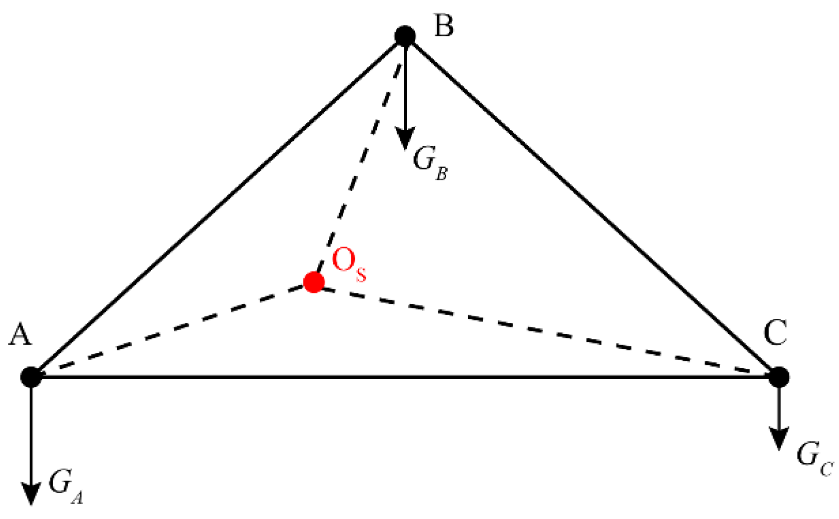
If the importance degree of a station is regarded as its ‘gravity’, the more important the station is, the more ‘gravity’ it has in the network. In this paper, following the calculation principle of the gravity center in physics, the concept of gravity center of stations’ importance in a network is proposed. An urban rail transit network is usually regarded as a planar network. If the stations with different importance are assigned to certain values and locations, the distribution of stations can be expressed in the form of scatter in the network. The equilibrium gravity point of the scatter in the planar topological network is the gravity center of the stations’ importance distribution, as shown in Figure 1. In Figure 1, $G_A$, $G_B$ and $G_C$ are the ‘gravity’ of station A, B and C, respectively, and the point ${\mathrm{O}}_{\mathrm{S}}$ is the gravity center. The calculation method of the coordinates of ${\mathrm{O}}_{\mathrm{S}}$ is shown in Equations (5)–(6):

$${\overline{x}}_1=\frac{{\displaystyle \sum _{i=1}^n{x}_i{I}_i}}{{\displaystyle \sum _{i=1}^n{I}_i}}$$

(5)

$${\overline{y}}_1=\frac{{\displaystyle \sum _{i=1}^n{y}_i{I}_i}}{{\displaystyle \sum _{i=1}^n{I}_i}}$$

(6)

where $({\overline{x}}_1,{\overline{y}}_1)$ is the coordinate pair of the gravity center of stations’ importance, $n$ is the number of stations in urban rail transit network, $(x_i,y_i)$ is the coordinate pair of station $i$.

The gravity center reflects the emphasis of rail transit development on urban spatial location. The location of the gravity center will change with the development of rail transit, and the focus area of the center reflects the importance of the urban area to a certain extent. The index will be used to calculate the matching degree between the network and the urban trips.

2.1.3. Fractal Dimension

Fractal theory originated in the late 1960s and was founded by Mandelbrot, B [21]. The theory was originally used to describe highly irregular graphics. Fractal dimension is the most important parameter of fractal theory. It is used to describe the dimension of complex irregular graphics, which is the measure of spatial scale and overall complexity of the graphics. In 1991, L. Benguigui and M. Daoud [22] inspected the railway system in the suburb of Paris and found that the railway network showed a branched fractal structure. After that, the fractal theory was gradually applied in the field of transportation.

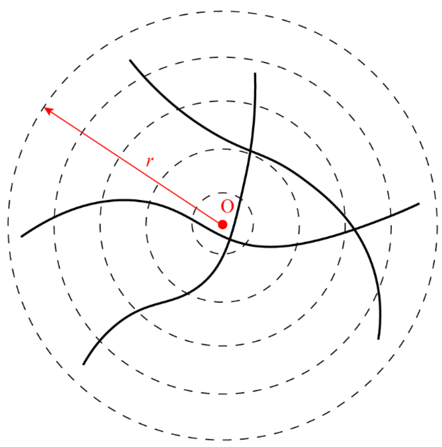
In fact, there are fractal features in a certain space–time range between the city and the transportation network systems, and their fractal geometry properties reflect the self-similar characteristics of the systems. In this paper, the city is regarded as a circular area, and the radius is centered around the urban center. Figure 2 shows the urban rail transit lines in the city with radius $r$, where the point O represents the urban center. The sum of the structural importance degrees of all stations $I(r)$ within the radius $r$ is calculated by Equation (7):

$$I(r)={\displaystyle \sum _{i=1}^{n_r}{I}_i}(r)$$

(7)

where $I_i(r)$ is the structural importance degree of station $i$ within the radius $r$, $n_r$ is the number of stations within the radius $r$.

According to the fractal theory, $I(r)$ and $r$ satisfy the following relationship:

$$I(r)\propto r^{D_S}$$

(8)

where $D_S$ is the fractal dimension of the stations’ importance distribution.

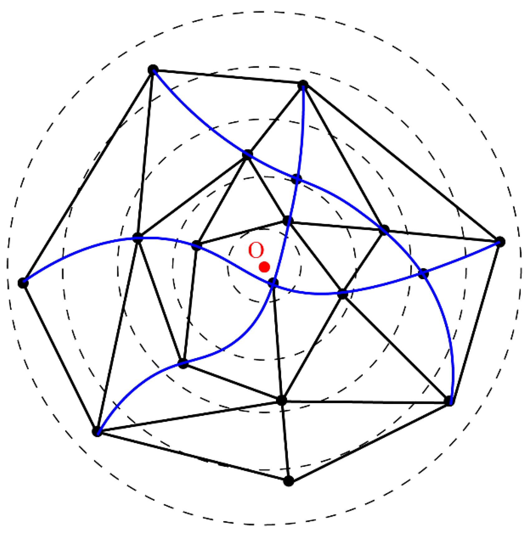
The city is divided into several circles by the radii with different lengths, and the stations with different importance are scattered in the circles. So the fractal dimensions corresponding to different radii can be obtained.

The fractal dimensions corresponding to different radii can reflect the change of rail transit supply capacity from an urban center to a peripheral area. In fact, the urban development is biased towards the central area, so the supply capacity of the central area is usually larger than that of the peripheral area. The index will be used to calculate the matching degree between the network and the urban land use.

2.2. Matching with Urban Characteristics

2.2.1. Urban Road Network

Usually, urban rail transit lines are laid along the roads, and only in special cases can be constructed through land blocks. Therefore, it is necessary to limit the roads, so as to determine the range and direction of the searchable sections when generating the network. In this way, not only the planner’s subjective and groundless decision can be avoided with mathematical model, but also reasonable route boundaries can be grasped. We refer to the topological network used to limit the search range and the search direction as the ‘basic network’.

The locations of large traffic volume and passenger flow corridors are the main factors affecting the line alignments and network structure. Among the factors, the locations with large traffic volume are the main source of production and attraction of passenger flow, including transportation hubs and centers of a district. The transportation hubs include a bus transfer hub, bus terminal, railway station and airport, etc. The centers of a district include commercial and cultural sites, large enterprises, large residential areas and tourist attractions, etc. So the basic network should be established by connecting the main locations of large traffic volume and covering the main passenger flow corridors. Before establishing the basic network, the main passenger corridors are determined by a ‘cobweb assignment’ method, and the steps are as follows:

Step 1: Generate OD (origin-destination) desire lines between traffic zones according to the predicted passenger demand.

Step 2: Eliminate the inter-zone desire lines while the desire lines between adjacent zones are retained. The network formed by the retained desire lines is called ‘virtual cobweb’.

Step 3: Passenger assignment is carried out on the ‘virtual cobweb’ with all-or-nothing method.

Step 4: Judging the main passenger flow corridors according to the scale of passenger flow accumulation.

Usually, most of the research on actual transit network designs are based on the premise that the basic network is known because of lacking effective determination method. Therefore, the determining process of the basic network proposed in this paper is as follows:

Step 1: Selection of trunk roads that meet the conditions for rail transit construction.

According to the urban traffic road network in the area requiring rail transit construction, the trunk roads along the passenger corridors and connecting the locations with large traffic volume are selected.

Step 2: Selection of other roads that can connect the locations of large traffic volume.

If the selected trunk roads cannot connect all the necessary locations of large traffic volume, other roads around the locations that meet the construction conditions and land-use requirements should be selected.

Step 3: The main locations of large traffic volume are connected along the selected roads, and the topology network formed is the basic network.

The locations with close distance and large traffic volume are merged. In this way, not only the complexity of solving the model, but also the detour distance of the generated transit lines can be reduced. Figure 3 shows the urban rail transit lines laid along the main routes in the basic network.

2.2.2. Trip Intensity

There is a certain difference for trip volumes in different traffic zones, and the volume in each zone includes the production and attraction of the trips. So, the trip intensity in each zone can be calculated by the amount of the production and attraction of the zone, as shown in Equation (9):

$$S_i=P_i+A_i$$

(9)

where $S_i$ is the trip intensity in traffic zone $i$, $P_i$ and $A_i$ are the production and attraction of trip volume in traffic zone $i$, respectively.

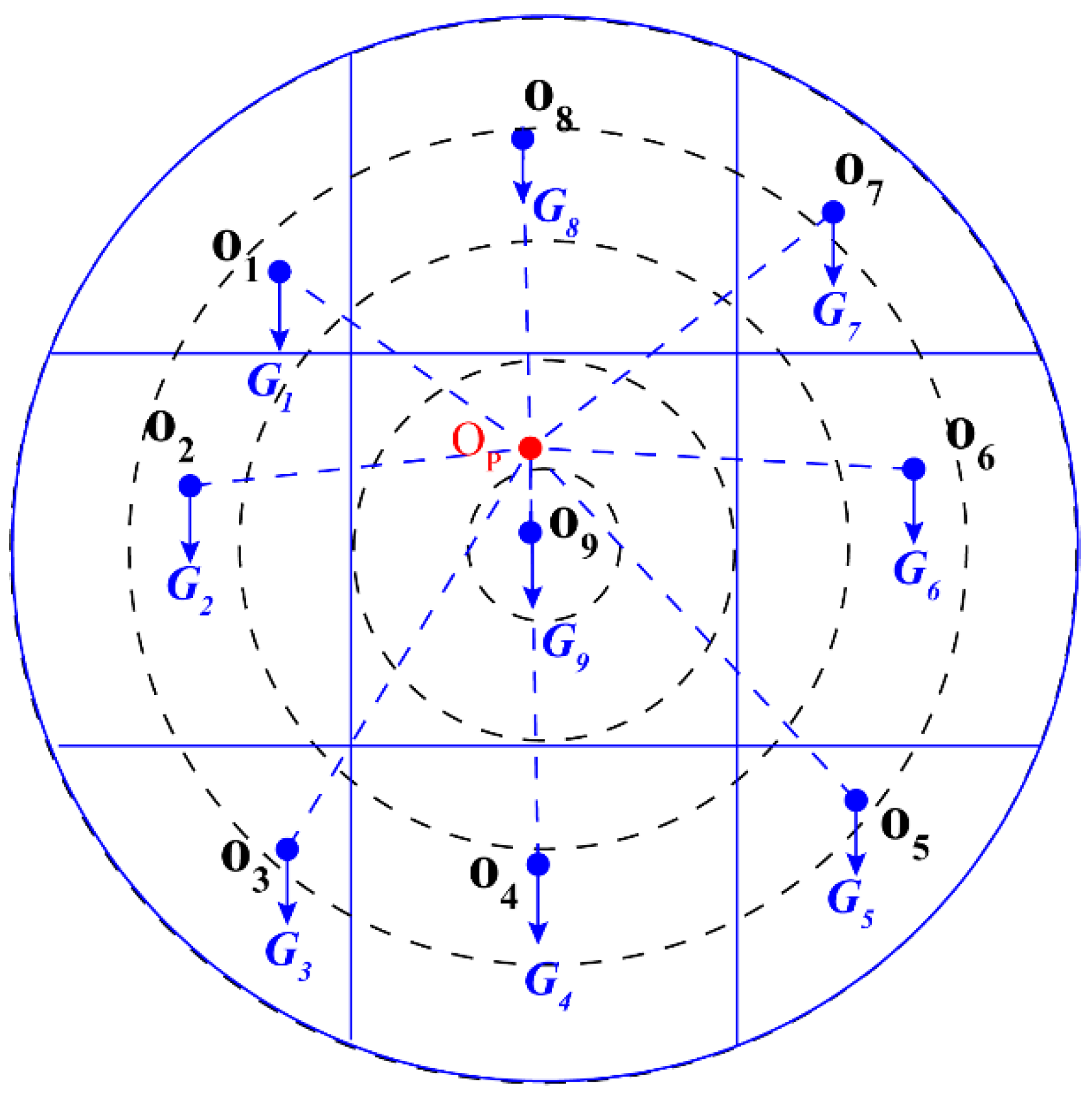
Usually, the trip intensity of each zone can be considered to be concentrated in the centroid position of the zone. So, if the centroid positions are assigned to corresponding trip-intensity values, the distribution of the trip volume can be expressed in the form of scatter in the city. Similarly, if the trip intensity of each zone is regarded as the ‘gravity’ of the zone, the equilibrium point of the ‘gravity’ is the gravity center of trip intensity, as shown in Figure 4. In Figure 4, each area represents the traffic zone, ${\mathrm{o}}_1{~\mathrm{o}}_9$ are the centroid positions of traffic zones, $G_1~G_9$ are the ‘gravity’ values, and ${\mathrm{O}}_{\mathrm{P}}$ is the gravity center of trip intensity. The coordinates of the gravity center can be calculated by Equations (10)–(11):

$${\overline{x}}_2=\frac{{\displaystyle \sum _{i=1}^m{x}_i{S}_i}}{{\displaystyle \sum _{i=1}^m{S}_i}}$$

(10)

$${\overline{y}}_2=\frac{{\displaystyle \sum _{i=1}^m{y}_i{S}_i}}{{\displaystyle \sum _{i=1}^m{S}_i}}$$

(11)

where $({\overline{x}}_2,{\overline{y}}_2)$ is the coordinate pair of the gravity center of urban trip intensity, $m$ is the number of traffic zones divided in the city, $(x_i,y_i)$ is the coordinate pair of centroid position of traffic zone $i$.

The gravity center of urban trip intensity reflects the bias in the distribution of urban trip volume. If the trip intensity in an area increases, the gravity center will develop toward the area. On the contrary, if the trip intensity decreases, the development direction of the gravity center will be reversed.

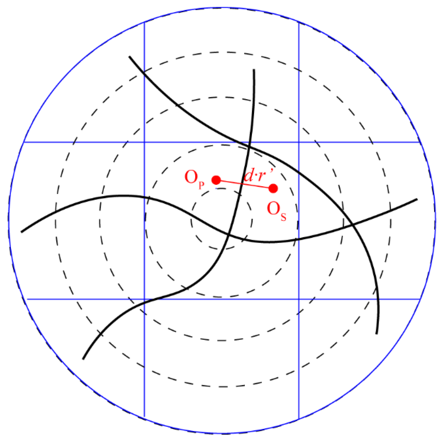
Urban rail transit is a main transportation mode for the residents in the city. The rail transit network should not only satisfy the capacity demand of passenger transport, but also match the distribution of trip volume in the city. So the importance distribution of rail transit stations should match the different trip volume in traffic zones. In this paper, the deviation value between the gravity center ${\mathrm{O}}_{\mathrm{P}}$ of urban trip intensity and the gravity center ${\mathrm{O}}_{\mathrm{S}}$ of stations’ importance distribution is used to characterize the matching degree between the network and urban trips, as shown in Figure 5. The deviation value is expressed as the ratio of Euclidean distance between ${\mathrm{O}}_{\mathrm{P}}$ and ${\mathrm{O}}_{\mathrm{S}}$ to urban radius, as shown in Equation (12).

$$d(O_P,O_S)=\frac{\sqrt{{({\overline{x}}_1-{\overline{x}}_2)}^2+{({\overline{y}}_1-{\overline{y}}_2)}^2}}{r\prime }$$

(12)

where $d$ is the deviation value of gravity centers between the stations’ importance distribution and the trip intensity, $r\prime$ is the radius calculated from the total area $A(r\prime )$ of the city, satisfying $A(r\prime )=\pi r{\prime }^2$.

Furthermore, the matching degree $m_C$ between urban rail transit network and urban trips can be calculated by Equation (13). The value of $m_C$ is between 0 and 1, and the closer the index value is to 1, the higher the matching degree between the network and urban trips.

$$m_C=\frac{1}{1+d(O_P,O_S)}$$

(13)

2.2.3. Land-Use Intensity

There is a feedback relationship between urban rail transit and land use. Land-use intensity is the root cause of passenger volume for urban rail transit while the rail transit could have a positive guiding role in the development of surrounding land use. Therefore, in the stage of network design, it is necessary to ensure the matching between the urban rail transit network and the land-use intensity [23].

Land-use intensity directly affects the accumulation of urban population, so it can be calculated by the population size within the area. Similarly, according to fractal theory, the relationship between the radius $r$ of the urban area and the land-use intensity satisfies Equation (14):

$$P(r)\propto r^{D_P}$$

(14)

where $P(·)$ is the land-use intensity calculated by the sum of resident and employed population, ${\mathrm{D}}_P$ is the fractal dimension of the land-use intensity.

Deriving $r$ on both sides of Equation (14), we can obtain Equation (15):

$$\frac{dP(r)}{dr}\propto D_p{r}^{D_P-1}$$

(15)

The area of the circle with radius $r$ is $A(r)=\pi r^2$, satisfying $dA(r)/dr=2\pi r$, so the land-use intensity per unit area $\rho (r)$ can be obtained from Equation (16):

$$\rho (r)=\frac{dP(r)}{dA(r)}\propto D_p{r}^{D_P-2}$$

(16)

As can be seen from Equation (16), when $D_p<2$, $\rho (r)\propto D_p{(1/r)}^{\left|D_P-2\right|}$, and as the statistical area expands with the increased radius $r$, $\rho (r)$ gradually decreases from the city center to the periphery of the city. When $D_p=2$, $\rho (r)$ remains unchanged. When $D_p>2$, $\rho (r)$ gradually increases from the city center to the periphery of the city. Therefore, the fractal dimension $P(r)$ reflects the changing trend of urban land-use intensity from the city center to the periphery of the city.

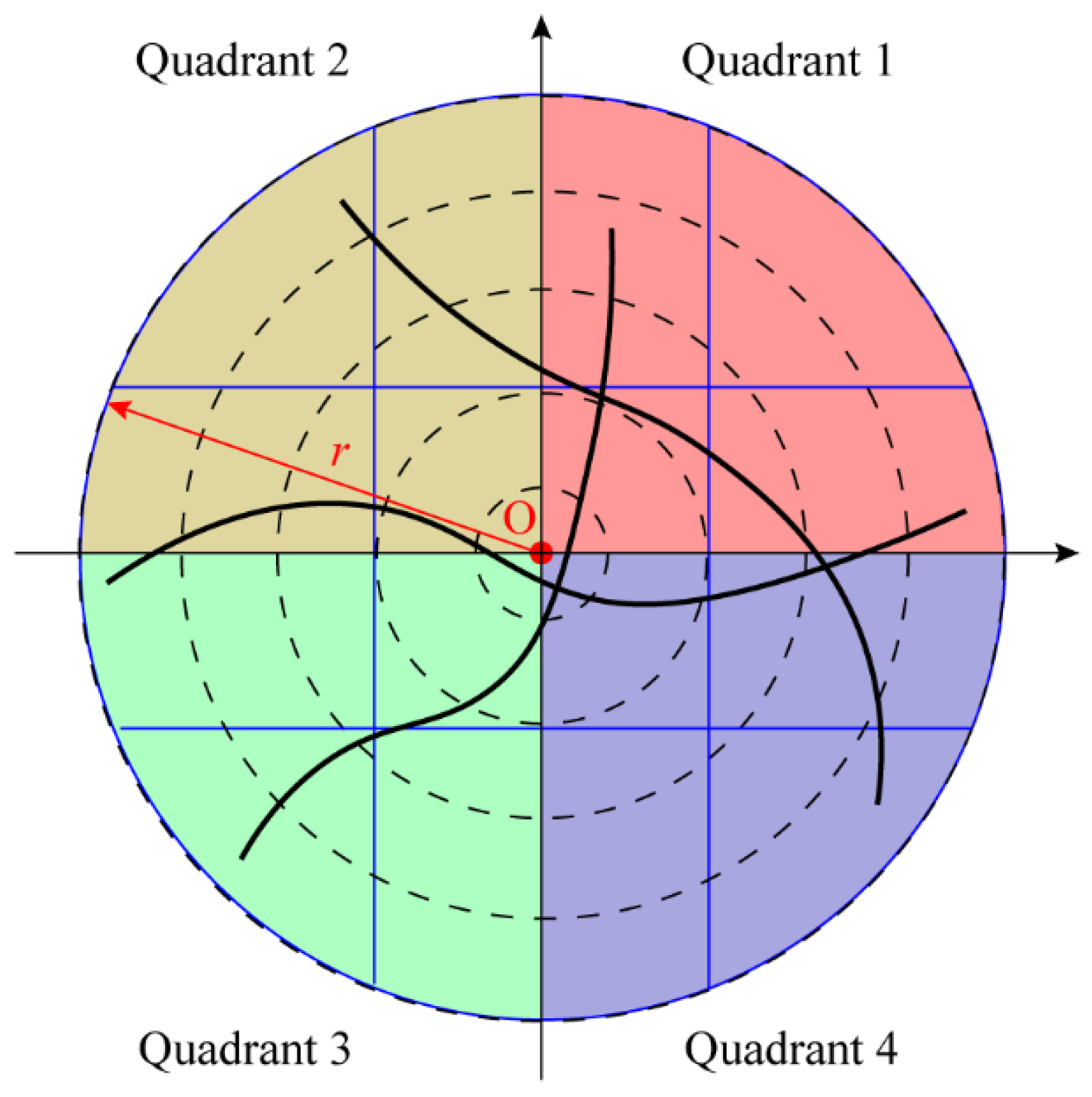
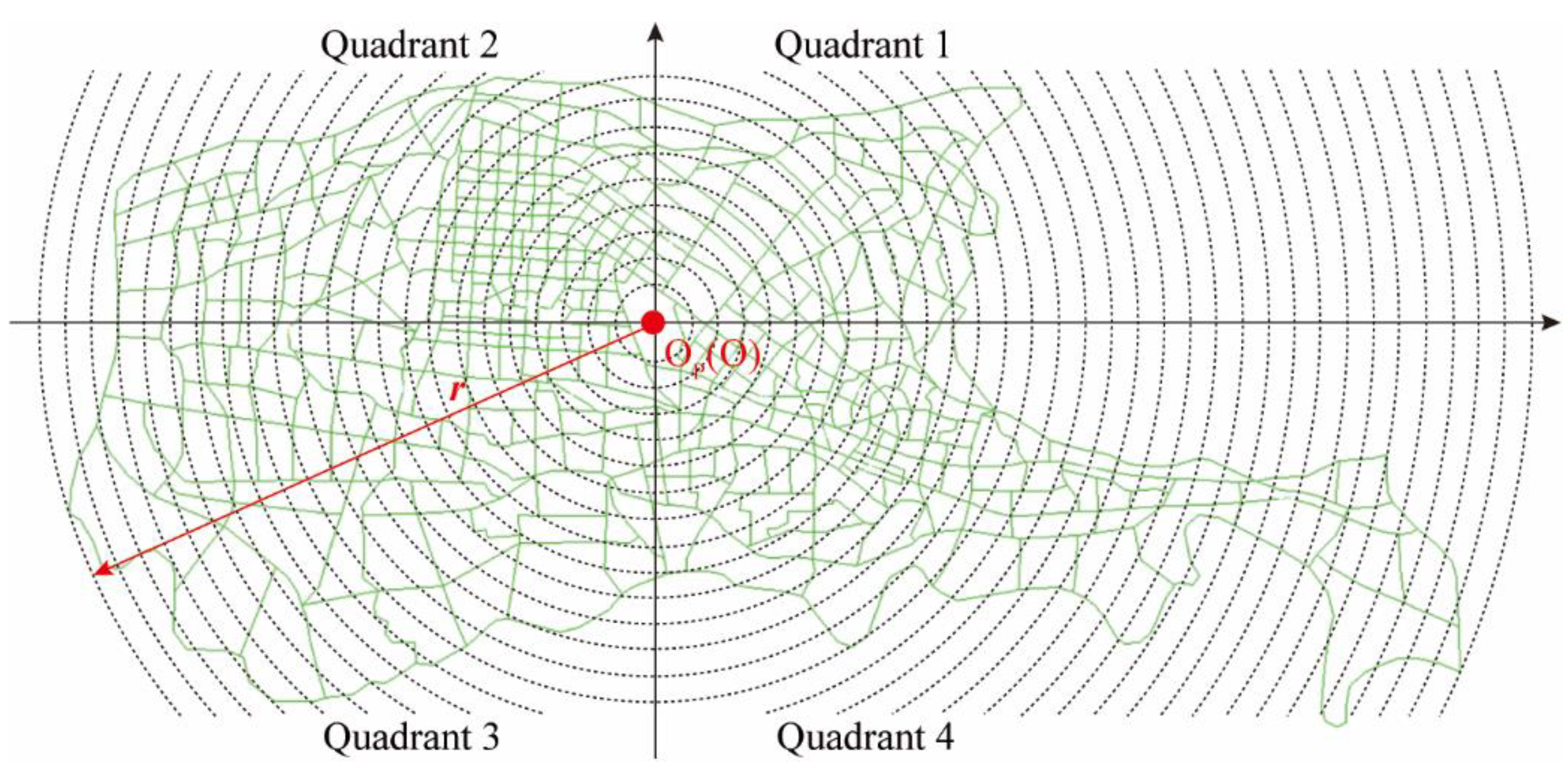
However, the city does not develop evenly in all directions. Therefore, in this paper, the city is divided into several fan-shaped areas in the radial direction. The fractal dimension of land-use intensity in each fan-shaped area should be calculated. If the city is divided into $m\prime$ areas (as seen in Figure 6, the city is divided into four fan-shaped areas using four quadrants.), the fractal dimension of land-use intensity in different areas can be expressed by the vector $[D_1,D_2,D_3,\dots ,D_{m\prime }]$, where the subscript number of the vector element represents the area number. So, the fractal dimension vector $D_S$ of stations’ importance distribution and the fractal dimension vector $D_P$ of land-use intensity can be expressed as $[D_{S1},D_{S2},D_{S3},\dots ,D_{Sm\prime }]$ and $[D_{P1},D_{P2},D_{P3},\dots ,D_{Pm\prime }]$, respectively, where ${\mathrm{D}}_{Si}$ is the fractal dimension of stations’ importance distribution in area $i$, ${\mathrm{D}}_{Pi}$ is the fractal dimension of land-use intensity in area $i$, $i=1,2,\dots m\prime$. The deviation value between $D_S$ and $D_P$ is used to describe the matching between the network and urban land use, as shown in Equation (17):

$$d(D_S,D_P)=\frac{\sqrt{{\displaystyle \sum _{i=1}^{m\prime }{(D_{Si}-D_{Pi})}^2}}}{m\prime }$$

(17)

where $d(D_S,D_P)$ is the deviation value of fractal dimensions between the stations’ importance distribution and the land-use intensity.

Therefore, the matching degree $m_F$ between the network and land use can be expressed by Equation (18). The value of $m_F$ is between 0 and 1, and the closer the index value is to 1, the higher the matching degree between the network and the land use.

$$m_F=\frac{1}{1+d(D_S,D_P)}$$

(18)

3. Model Formulation

3.1. Notations

The station and section of urban rail transit are abstracted as node $i$ in $N$ and edge $\{i,j\}$ in $E$, respectively. The topological network for urban rail transit is established, which is expressed as $G=G(N,E)$. The notations in the model are shown in

Table 1. Sets in the model.

Sets	Meaning
$L$	The set of lines of the candidate network, satisfying $l\in L$.
$E$	The set of sections of the basic network, satisfying $\{i,j\}\in E$.
$N$	The set of stations of the basic network, satisfying $i,j\in N$.
$N(i)$	The set of adjacent points of station $i$.
$W$	The set of OD pairs between the locations of large traffic volume, satisfying $w\in W$.
$N_p$	The set of effective paths between OD pairs, satisfying $p\in N_p$.

,

Table 2. Known quantities in the model.

Notations	Meaning
$d_{ij}$	The length of section $\{i,j\}$.
$g_w$	The passenger demand between OD pair $w$.
$N_{nodes\min }^l$	The minimum number of stations of line $l$ in the candidate network.
$N_{nodes\max }^l$	The maximum number of stations of line $l$ in the candidate network.
$d_{\min }^l$	The minimum length of line $l$ in the candidate network.
$d_{\max }^l$	The maximum length of line $l$ in the candidate network.
$N_l{}_{\min }$	The minimum number of lines in the candidate network.
$N_l{}_{\max }$	The maximum number of lines in the candidate network.
$C_{ij}$	The capacity of section $\{i,j\}$.
$x_i$	The abscissa of station $i$.
$y_i$	The ordinate of station $i$.
$a$	The station repeatability, satisfying $a>0$ and $a$ is an integer.
$b$	The section repeatability, satisfying $b>0$ and $b$ is an integer.
$c$	The minimum angle between adjacent sections in a line.
$m_{C\min }$	The minimum matching degree between the network and urban trips.
$m_{F\min }$	The minimum matching degree between the network and land-use intensity.

and

Table 3. Variables in the model.

Variables	Meaning
$e_{ij}$	If the candidate network has the section $\{i,j\}$, $e_{ij}=1$, 0 otherwise.
$e_{ij}^l$	If the line $l$ in the candidate network has the section $\{i,j\}$, $e_{ij}^l=1$, 0 otherwise.
$v_i$	If the candidate network has the station $i$, $v_i=1$, 0 otherwise.
$v_i^l$	If the line $l$ in the candidate network has the station $i$, $v_i^l=1$, 0 otherwise.
$f_{ij}^{wpl}$	If the OD pair $w$ passes the section $\{i,j\}$ of line $l$ along the path $p$, $f_{ij}^{wpl}=1$, 0 otherwise.
$f^{wpl{l}^{\prime }}$	If the OD pair $w$ transfers from line $l$ to line $l\prime$ along the path $p$, $f^{wpl{l}^{\prime }}=1$, 0 otherwise.
$q_{ij}$	The cross-sectional passenger volume of section $\{i,j\}$.
$P_{wp}$	The selection probability of path $p$ between OD pair $w$.

.

3.2. Objective Functions

In this paper, we focus on how to consider the characteristics of urban road network, trips and land use in the quantitative network design. So other factors involved in the model have to be simplified. The model is formulated based on the assumption that passenger demand for the urban rail transit is already known.

In this paper, the logit-based multi-path passenger flow assignment method is adopted. The utility function for path selection is expressed by passenger’s travel time which is the main influencing factor, as shown in Equation (19):

$$T_w^p=T_r^p+T_d^p+T_t^p,w\in W,p\in N_p$$

(19)

where $T_w^p$ is the travel time for OD pair $w$ along the path $p$, $T_r^p$ is the travel time in sections, $T_d^p$ is the dwell time at intermediate stations, $T_t^p$ is the transfer time.

During the trip, too many transfers will seriously affect the convenience for passengers, and thus reduce the attraction of the urban rail transit. In order to describe the influence of transfers, the transfer penalty is used for transfer time calculation, as shown in Equation (20):

$$T_t^p={\displaystyle \sum _k{T}_{tk}^p{(\lambda k+1)}^{\gamma }}$$

(20)

where $T_{tk}^p$ is the transfer time in the $k^{th}$ transfer station along the path $p$, $\lambda$ is the passenger’s transfer sensitivity, $\gamma$ is the adjustment coefficient which is usually larger than 1. The larger the $\gamma$, the greater the difference for sensitivity levels between different transfer times in the path.

The effective paths, which are defined by Equation (21), are searched for between each OD pair in the network. So the path selection probability $P_{wp}$ is calculated by Equation (22):

$$T_w^p\le (1+H)T_w^{p_{\min }}$$

(21)

where $H$ is the detour coefficient and is set to 1.5 in this paper, $T_w^{p_{\min }}$ is the travel time in the shortest path.

$$P_{wp}=\frac{\exp (-\theta T_w^p)}{{\displaystyle \sum _{p\in N_p}\exp (-\theta T_w^p)}},w\in W,p\in N_p$$

(22)

where $\theta$ is the calibration parameter.

As a kind of public transport, urban rail transit should not only achieve the purpose of profitability for the managers, but also take into account the service function to meet passengers’ demand. In this paper, the objective functions are formulated from the perspective of both managers and passengers to improve the transport efficiency of the network and the convenience for passengers.

Objective 1: Maximize the transport efficiency of the network

From the managers’ point of view, the network should transport as much passengers as possible to improve the operating income. Passenger turnover quantity refers to the product of the passenger volume and the distance transported in a certain period of time, and the unit is $p·km$. The larger the passenger turnover quantity, the higher the transport capacity of the network. Therefore, the passenger turnover quantity per unit length of the network is used to characterize the transport efficiency, which is expressed by Equation (23):

$$\max Z_1=\frac{{\displaystyle \sum _{\{i,j\}\in E}{q}_{ij}{d}_{ij}{e}_{ij}}}{{\displaystyle \sum _{\{i,j\}\in E}{d}_{ij}{e}_{ij}}}$$

(23)

Objective 2: Maximize the travel convenience for passengers

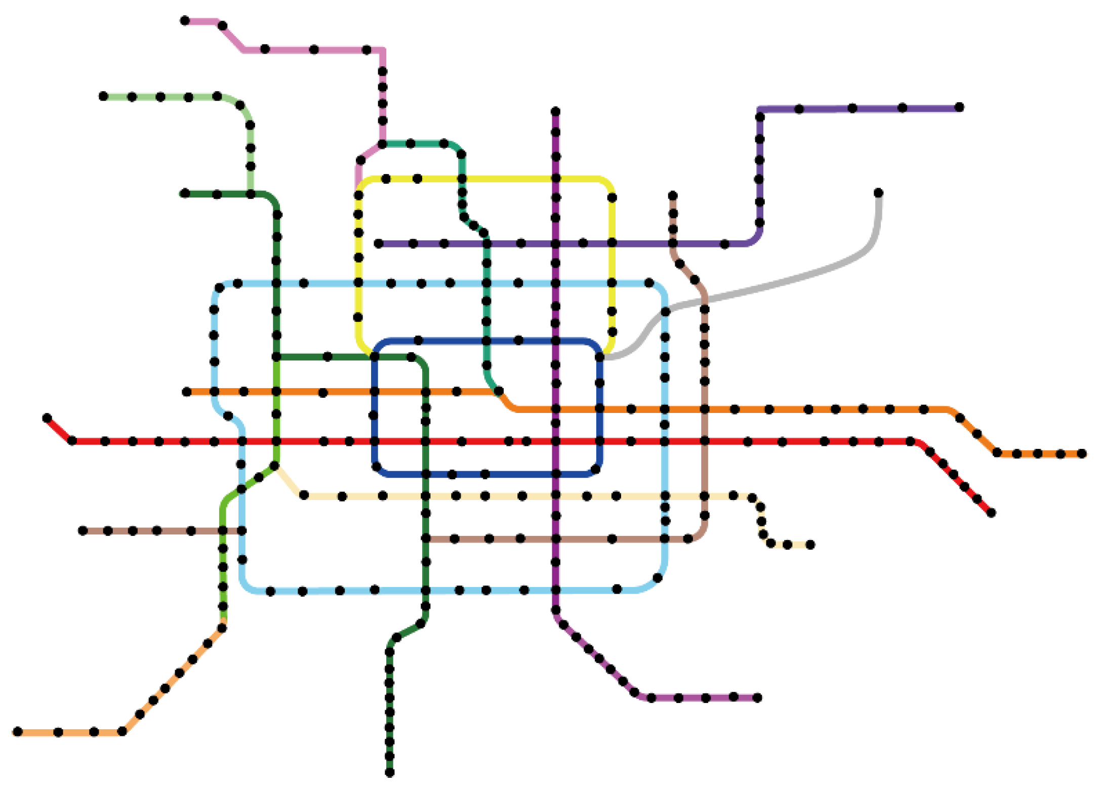
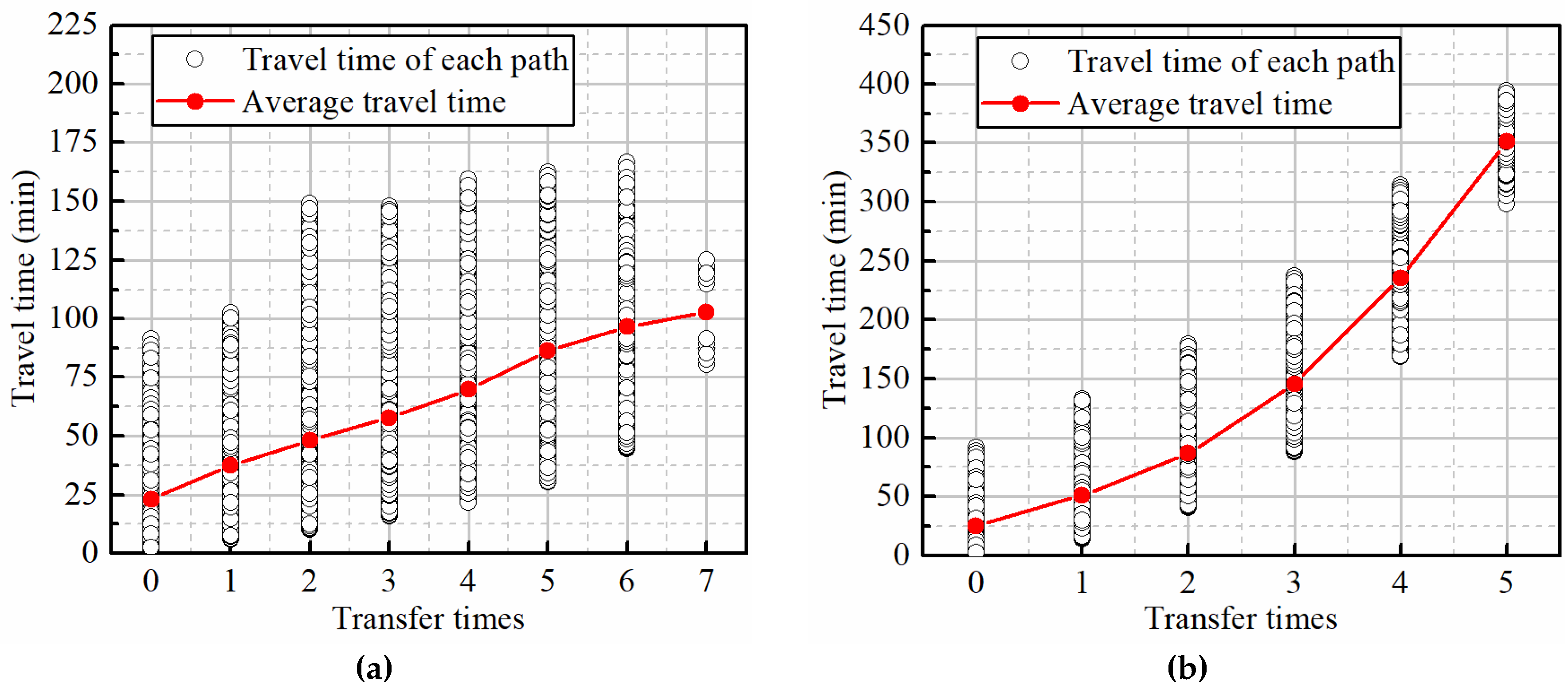
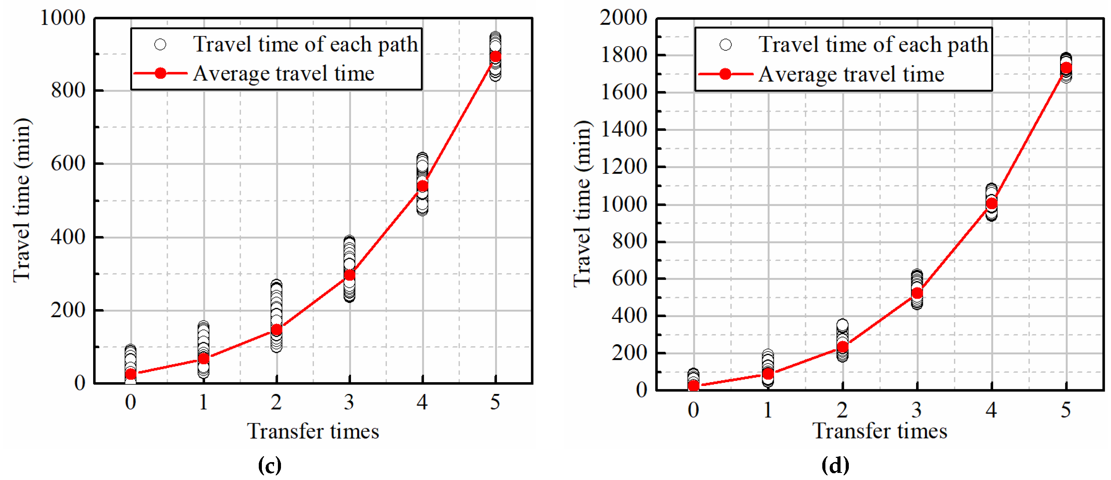
In order to explore the relationship between the transfer times and the travel time in paths, the effective paths between each OD pair in the metro network of Beijing (as shown in Figure 7) are calculated, and the results are shown in Figure 8. As can be seen, a path with more transfer times tends to have more average travel time, and the greater the transfer sensitivity, the more obvious the phenomenon. Therefore, the average travel time of all passengers can be reduced while the average transfer times in paths are reduced.

In order to improve the travel convenience for passengers, it is necessary to improve the directness of traveling for passengers. Reducing the transfer times for passengers is a very effective method to achieve this. Therefore, the average number of transfer passengers between lines is used as the second objective, which is expressed by Equation (24):

$$\min Z_2=\frac{{\displaystyle \sum _{w\in W}{\displaystyle \sum _{l,l\prime \in L,l\ne l\prime }{\displaystyle \sum _{p\in N_p}{g}_w{P}_{wp}{f}^{wpl{l}^{\prime }}}}}}{\left|L\right|(\left|L\right|-1)/2}$$

(24)

Both the two objectives have the same unit, so the problem can be easily converted into a single objective problem with weighted sum approach for the convenience of solving. The transformed objective function is shown in Equation (25):

$$\max \mathrm{Z}={\beta }_1{\mathrm{Z}}_1-{\beta }_2{\mathrm{Z}}_2$$

(25)

where ${\beta }_1+{\beta }_2=1$, satisfying $0\le {\beta }_1\le 1$, $0\le {\beta }_2\le 1$.

3.3. Constraints

Constraint 1: Network topological relationship.

$$e_{ij}^l\le v_i^l,l\in L,i\in N,\{i,j\}\in E$$

(26)

$$e_{ij}^l\le v_j^l,l\in L,j\in N,\{i,j\}\in E$$

(27)

$$e_{ij}^l=e_{ji}^l,l\in L,\{i,j\}\in E$$

(28)

$$e_{ij}\le {\displaystyle \sum _{l\in L}{e}_{ij}^l},l\in L,\{i,j\}\in E$$

(29)

$$e_{ij}^l\le e_{ij},l\in L,\{i,j\}\in E$$

(30)

$${\displaystyle \sum _{j\in N(i)}{e}_{ij}^l}\le 2,l\in L,\{i,j\}\in E$$

(31)

$$\frac{1}{2}{\displaystyle \sum _{\{i,j\}\in \mathrm{E}}{e}_{ij}^l}+1={\displaystyle \sum _{i\in N}{v}_i^l},l\in L$$

(32)

$${\displaystyle \sum _{l\in L}{v}_i^l}\le a,i\in N,\{i,j\}\in E$$

(33)

$${\displaystyle \sum _{l\in L}{e}_{ij}^l}\le b,\{i,j\}\in E$$

(34)

Equations (26) and (27) indicate that if the station $i$ or station $j$ is not on the line $l$, the section $\{i,j\}$ will not on the line $l$. Equation (28) indicates that the network is regarded as undirected graph. Equations (29) and (30) indicate that if the network has the section $\{i,j\}\in E$, multiple lines in the network are allowed to pass through the section $\{i,j\}$. Equations (31) and (32) indicate that the line $l$ has neither branches nor loops. Equation (33) indicates that there are up to $a$ lines have the station $i$ in the network. Similarly, Equation (34) indicates that there are up to $b$ lines have the section $\{i,j\}$.

Constraint 2: Passenger flow balance.

$${\displaystyle \sum _{l\in L}{\displaystyle \sum _{i:\{i,k\}\in E}{f}_{ik}^{wpl}}-}{\displaystyle \sum _{l\in L}{\displaystyle \sum _{j:\{k,j\}\in E}{f}_{kj}^{wpl}}=}\{\begin{array}{l}-1,k\in O^w\\ 1,k\in D^w\\ 0,else\end{array},w\in W,p\in N_p$$

(35)

$$f_{ij}^{wpl}+f_{ji}^{wpl}\le e_{ij}^l,l\in L,\{i,j\}\in E,w\in W,p\in N_p$$

(36)

Equation (35) indicates that for OD pair $w$, if station $k$ is the departure station $O^w$, there is only the inflow at the station; if station $k$ is the intermediate station, the inflow is equal to the outflow at the station; if station $k$ is the terminal station $D^w$, there is only outflow at the station. Equation (36) indicates that there is no backflow in the line $l$.

Constraint 3: Matching degrees between network and urban characteristics.

$$m_{C\min }\le m_C\le 1$$

(37)

$$m_{F\min }\le m_F\le 1$$

(38)

Equations (37) and (38) indicate that the matching degrees $m_C$ and $m_F$ should meet the upper and lower limits, respectively.

Constraint 4: Line alignments.

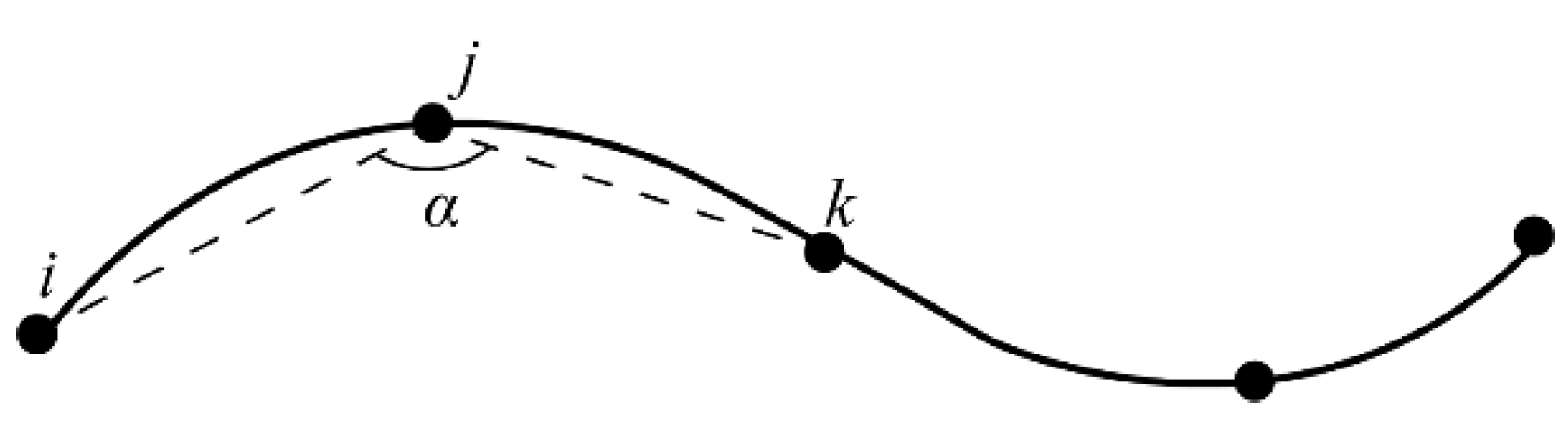
In Figure 9, $i$, $j$ and $k$ represent three adjacent stations in line $l$. $\alpha$ is the angle between the vectors $\overrightarrow{ji}$ and $\overrightarrow{jk}$. In order to ensure the line alignment goes smoothly, the angle $\alpha$ between the adjacent sections should not be too small, as seen in Equation (39).

$$c\le \alpha \le \pi$$

(39)

The cosine of the angle between the vectors $\overrightarrow{ji}$ and $\overrightarrow{jk}$ can be easily calculated by Equation (40). So Equation (39) can be expressed by Equation (41).

$$\cos \alpha =\frac{(x_i-x_j)(x_k-x_j)+(y_i-y_j)(y_k-y_j)}{\sqrt{{(x_i-x_j)}^2+{(y_i-y_j)}^2}\sqrt{{(x_k-x_j)}^2+{(y_k-y_j)}^2}}$$

(40)

where $(x_i,y_i)$, $(x_j,y_j)$ and $(x_k,y_k)$ are the coordinate pairs of station $i$, j and $k$, respectively.

$$c\le \arccos \alpha \le \pi$$

(41)

Constraint 5: Network size.

$$N_{nodes\min }^l\le {\mathrm{N}}_{nodes}^l\le N_{nodes\max }^l,l\in L$$

(42)

$$d_{\min }^l\le {\displaystyle \sum _{\{i,j\}\in E}{d}_{ij}}{e}_{ij}^l\le d_{\max }^l,l\in L$$

(43)

$$N_{l\min }\le \left|L\right|\le N_{l\max }$$

(44)

Equations (42)–(44) indicate that the number of stations in line $l$, the length of line $l$ and the number of lines in the network should meet the upper and lower limits, respectively, where ${\mathrm{N}}_{nodes}^l$ is the number of stations in the line $l$.

Constraint 6: Capacity of sections.

$${\displaystyle \sum _{w\in W}{\displaystyle \sum _{p\in N_p}{g}_w{P}_{wp}{f}_{ij}^{wpl}}}\le C_{ij},l\in L,\{i,j\}\in E$$

(45)

Equation (45) indicates that cross-sectional passenger volume of sections in each line is less than $C_{ij}$.

4. Neighborhood Search Algorithm

The problem dealt with in this paper is NP-hard. It has high structural complexity, multiple constraints and large search space, etc. So a neighborhood search algorithm [7] is developed based on a simulated annealing algorithm. A simulated annealing algorithm is a random optimization algorithm based on a Monte Carlo iterative solution strategy, and has strong robustness, global convergence and wide adaptability, which is suitable for solving the problem.

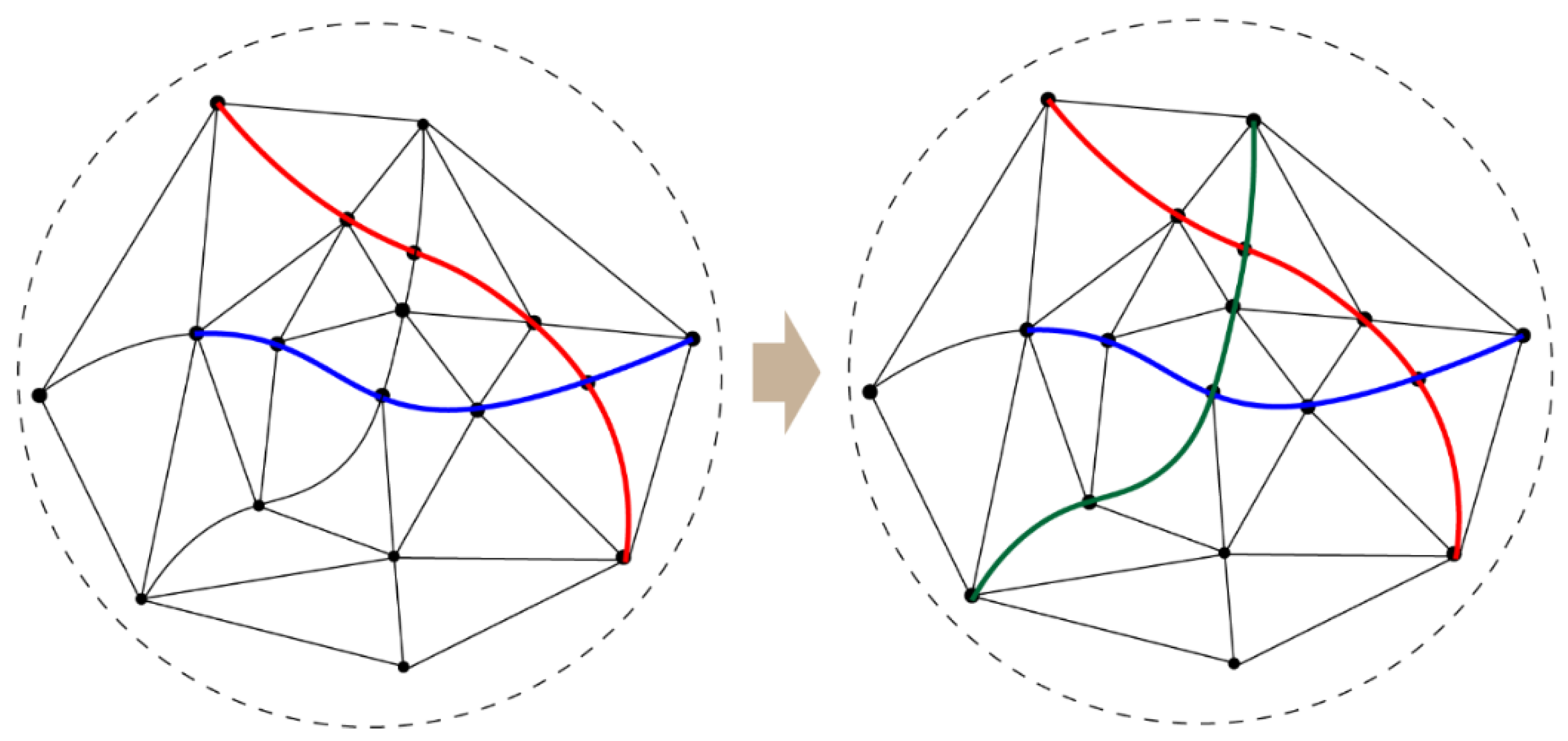
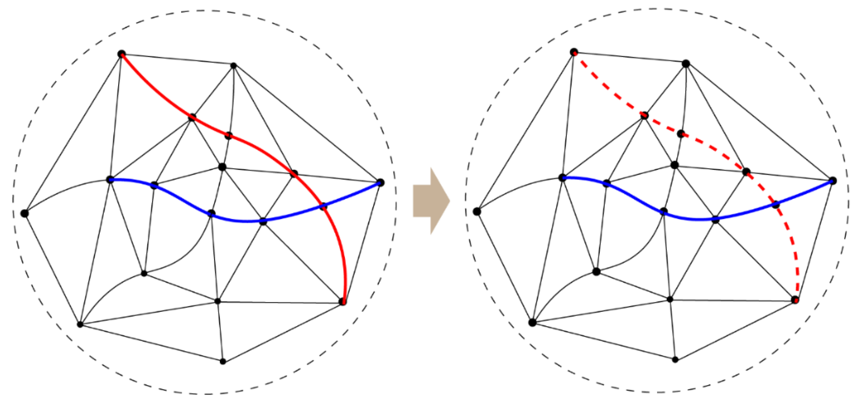
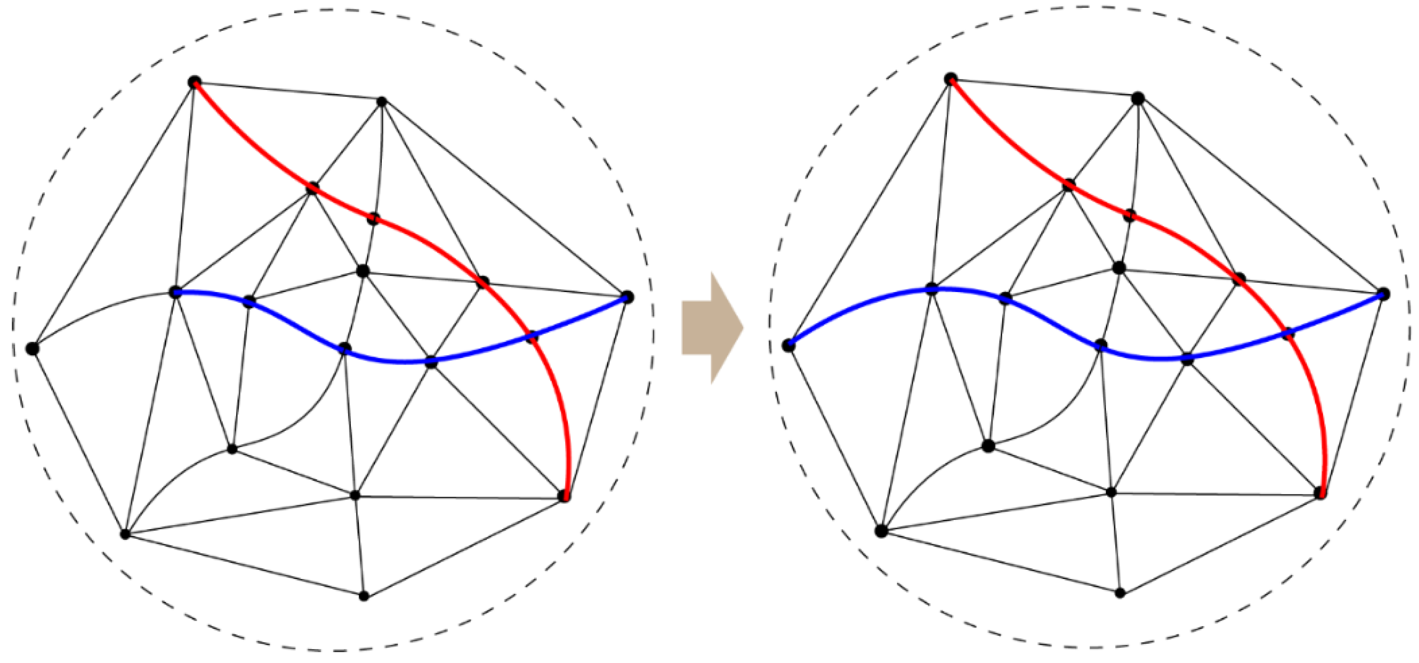
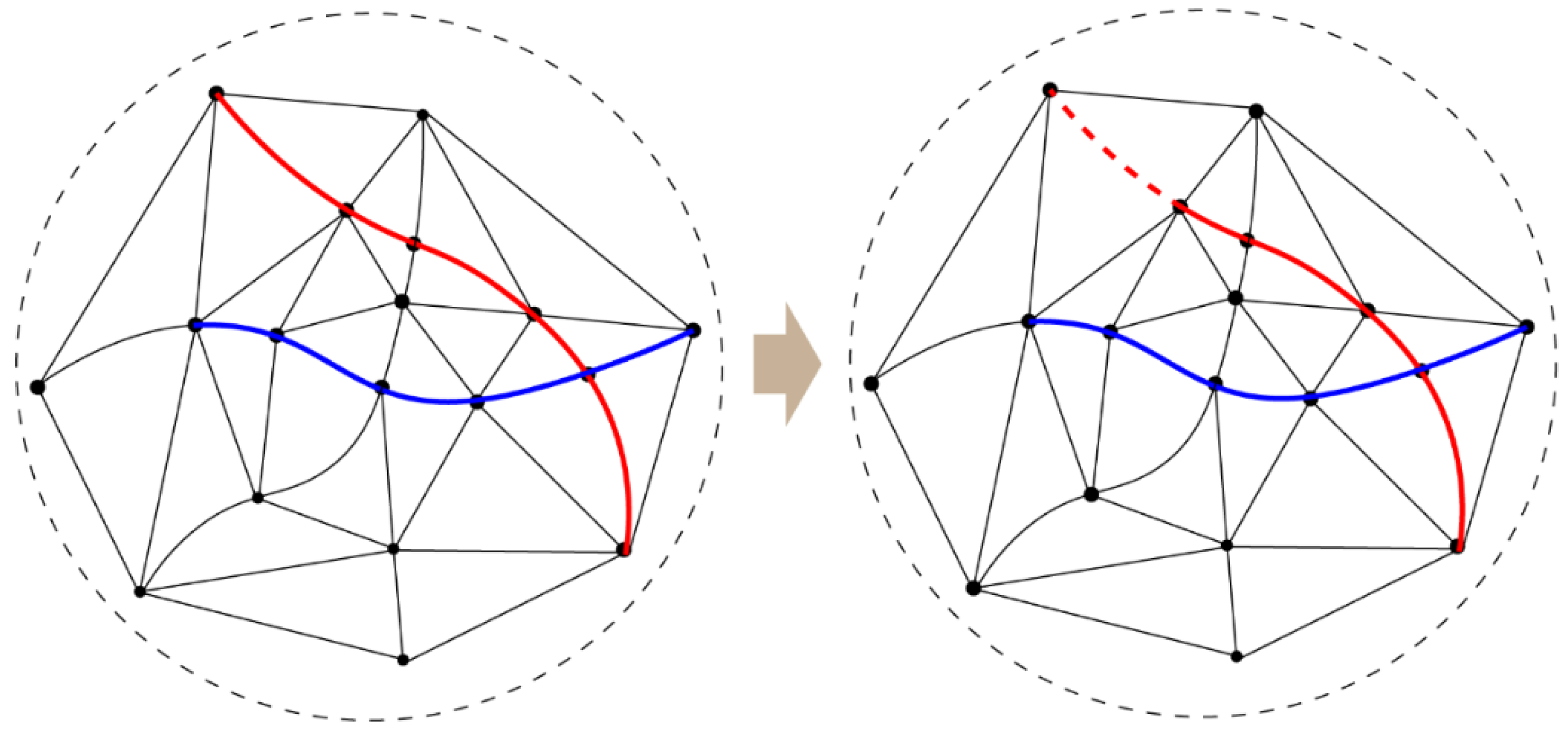
In order to obtain a variety of perturbation solutions in the iteration process, four neighborhood transform operators are designed. The functions of these operators are as follows: adding a line randomly, deleting a line randomly, adding a section in a line randomly and deleting a section in a line randomly, as shown in Figure 10, Figure 11, Figure 12 and Figure 13. Different neighborhood transform operators are executed according to a certain probability. Different types of perturbations are randomly applied to the current solution $G_{curr}$ to obtain new solution $G_{new}$. Each operator can be executed independently or simultaneously, for example, one line can be added while another line can be deleted at the same time.

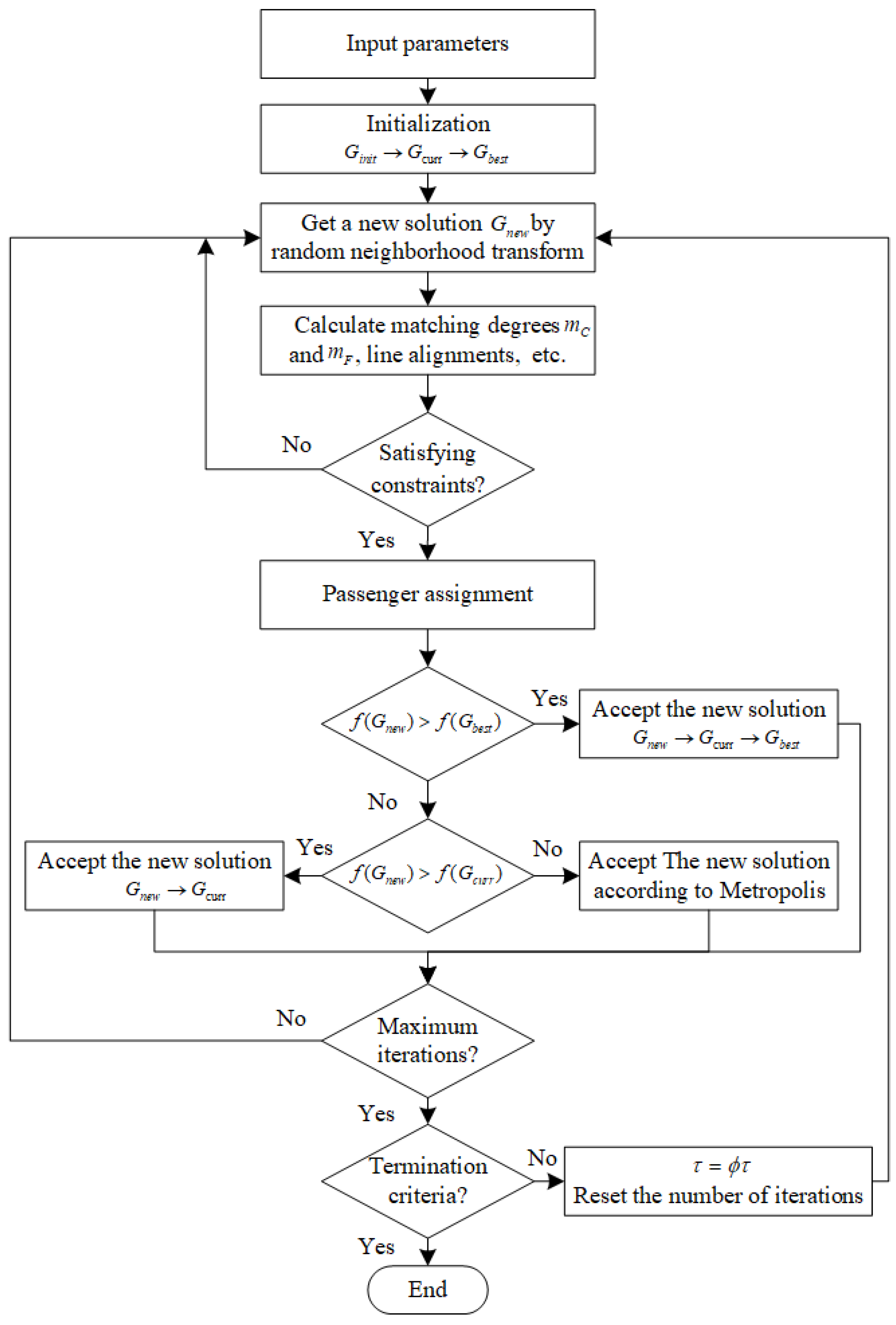
Let $f(G_{curr})$, $f(G_{new})$ and $f(G_{best})$ be the objective function values of the current solution $G_{curr}$, the new solution $G_{new}$ (perturbation solution) and the optimal solution $G_{best}$ in the existing iteration process, respectively. If $f(G_{new})>f(G_{curr})$, $G_{new}$ is accepted as the new current solution. Otherwise, $G_{new}$ is accepted according to the Metropolis criterion. Metropolis criterion is that the algorithm allows the inferior solution to be accepted with a certain probability, so that the algorithm can jump out of the trap of the local optimum. The acceptance probability in the criterion is calculated by Equation (46). As the temperature decreases, the probability of accepting an inferior solution decreases gradually.

$$p_r=e^{[f(G_{new})-f(G_{curr})]/\tau }$$

(46)

where $\tau$ is the current temperature.

The algorithm is designed with the memory function of the optimal solution $G_{best}$ in the existing iteration process, that is, to remember the ‘best so far’ state. As the iteration proceeds, the solution $G_{best}$ in the memory base is continuously updated until the algorithm converges. Therefore, the objective value will approach the global optimum gradually in the iterative process. A solution has many kinds of changes after perturbation, so even if the current solution is perturbed into the solution that has appeared in previous iterations, it will change in other directions when perturbed again, which will not have a negative impact on the results. The overall flow of the algorithm is shown in Figure 14.

5. Real-World Case Application

5.1. Basic Network

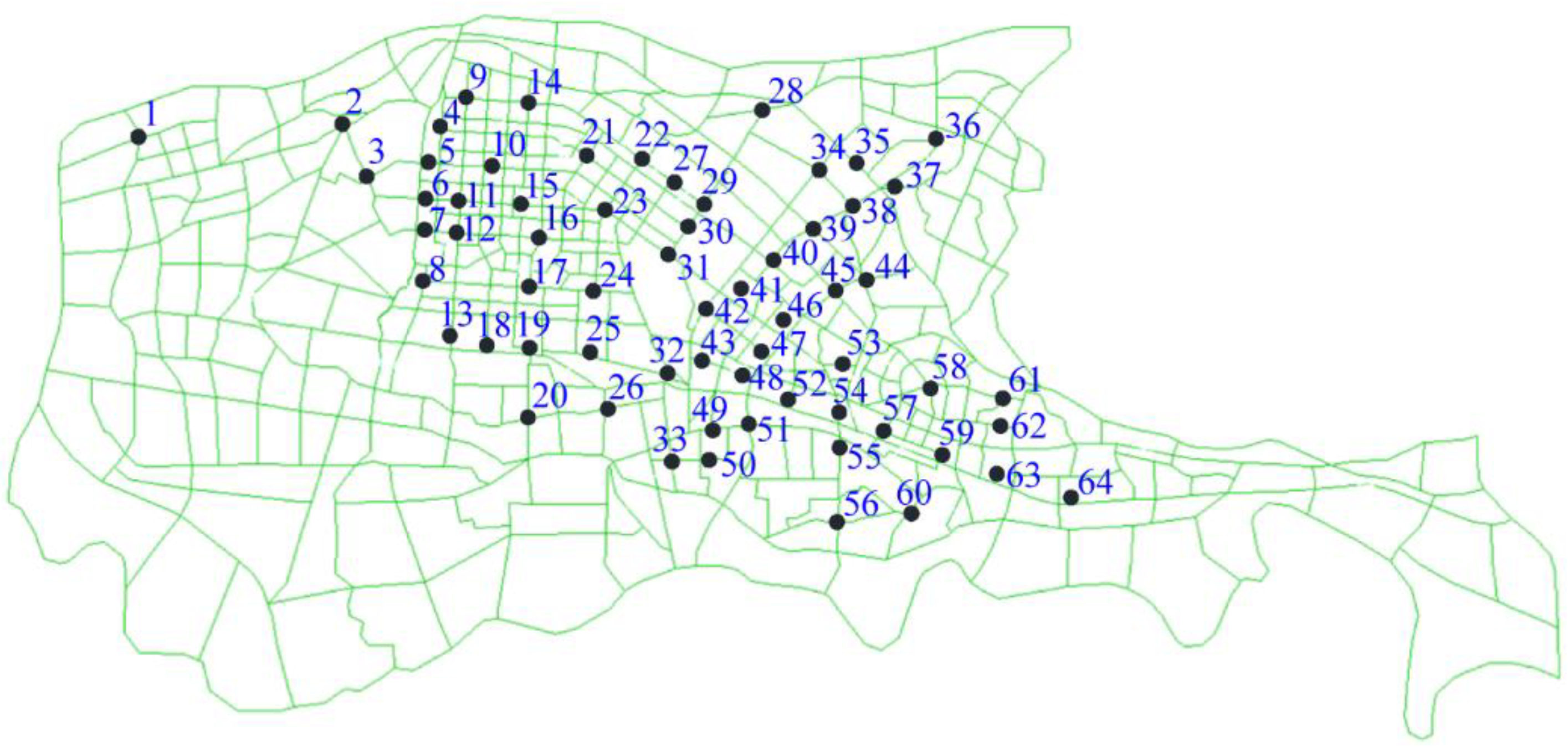
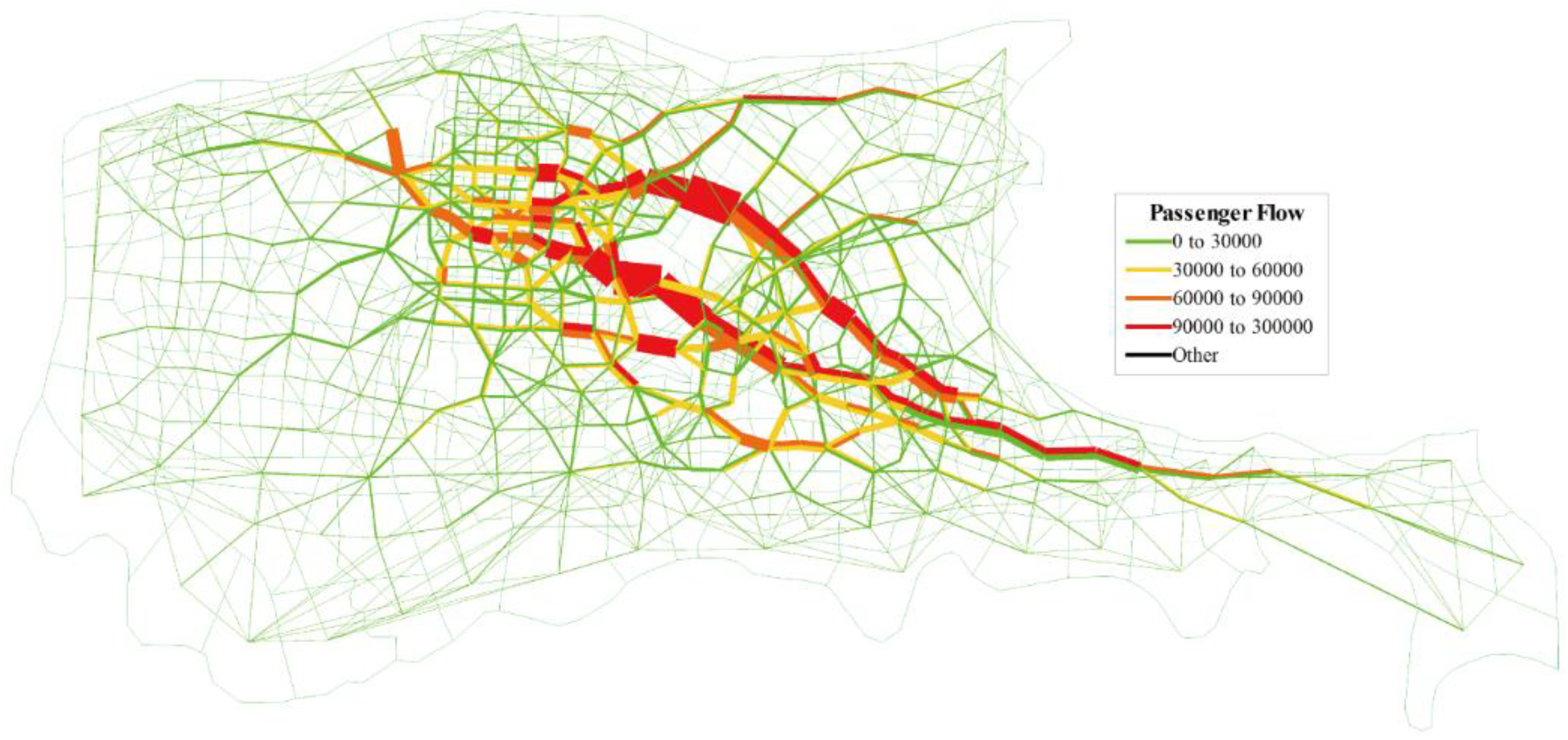
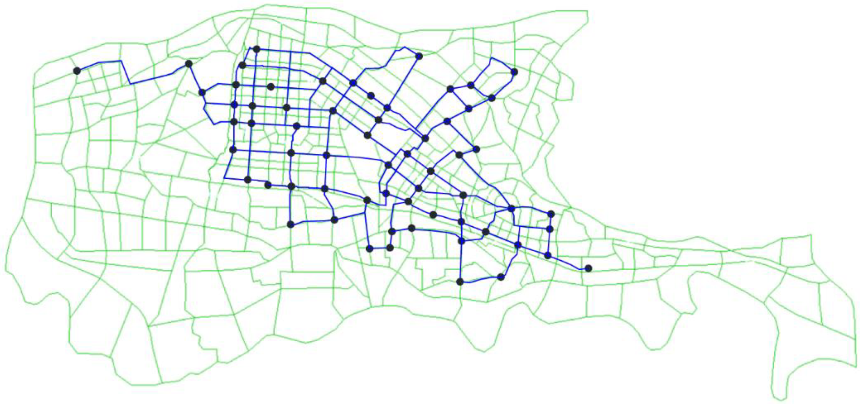
Baotou, which is a prefecture-level city in Inner Mongolia, has the total area of over 2000 square kilometers. The urban area was divided into 433 traffic zones, and 64 locations of large traffic volume were selected in the urban central area, as shown in Figure 15. The urban passenger corridors determined using the ‘cobweb assignment method’ are shown in Figure 16. As can be seen, the urban passenger corridors are mainly located in the east–west axis. According to the passenger corridors and the main axis of urban development, the basic network is formed using the method presented in Section 2.2.1, as shown in Figure 17.

5.2. Parameters

In the algorithm, the annealing rate $\varphi$ is set to 0.9, and the maximum number of iterations is set to 500. In this case, the passenger’s transfer sensitivity $\lambda$ is set to 0. The values of other parameters in the model are shown in

Table 4. Parameter values in the model.

Parameter	Value	Parameter	Value
${\beta }_1$	0.65	$N_{l\max }$	6
${\beta }_2$	0.35	$C_i{}_j$	45000
$N_{nodes\min }^l$	15	$a$	3
$N_{nodes\max }^l$	8	$b$	2
$d_{\min }^l$	15 km	$c$	$\frac{5}{12}\pi$
$d_{\max }^l$	35 km	$m_{C\min }$	0.7
$N_{l\min }$	3	$m_{F\min }$	0.65

.

5.3. Urban Characteristic Indexes

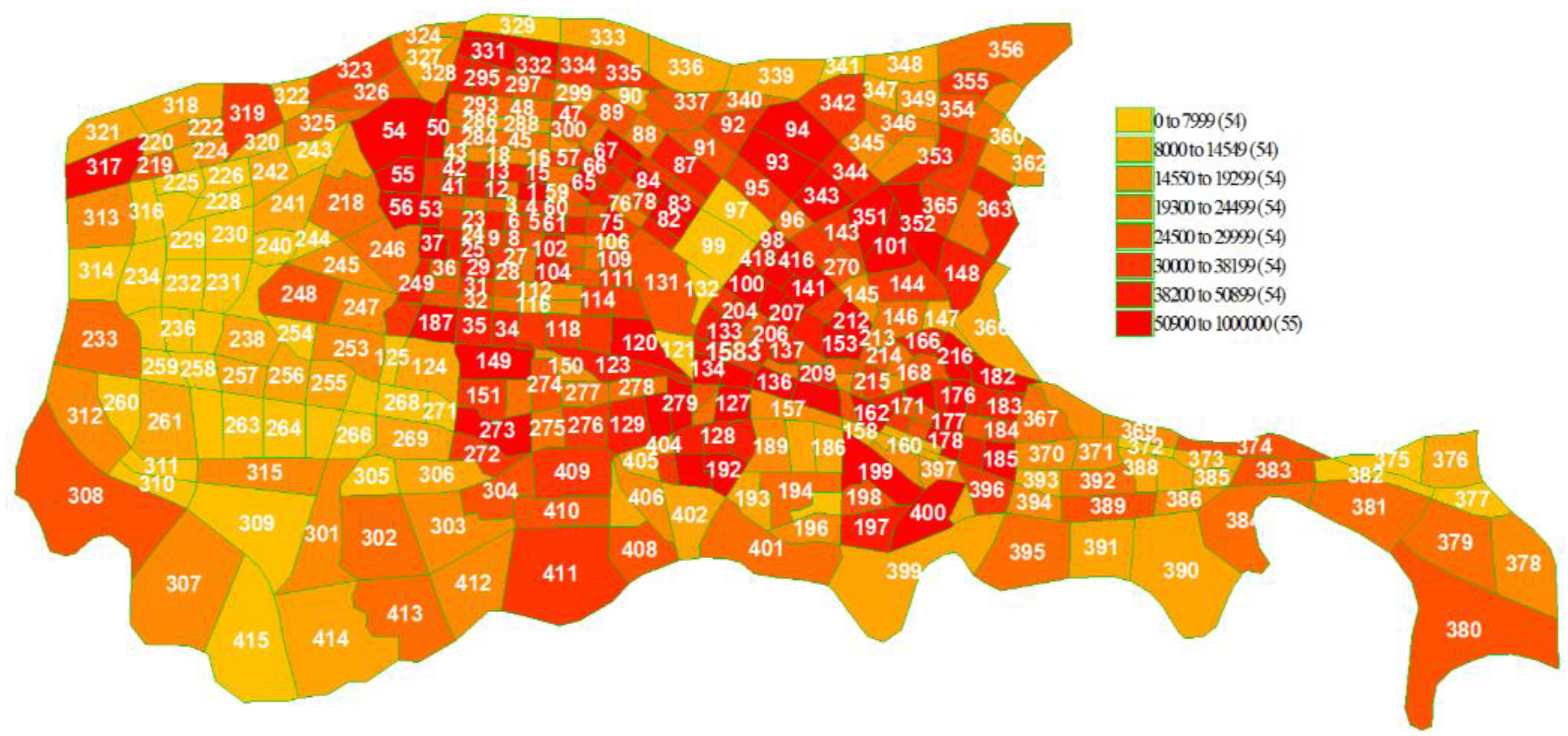
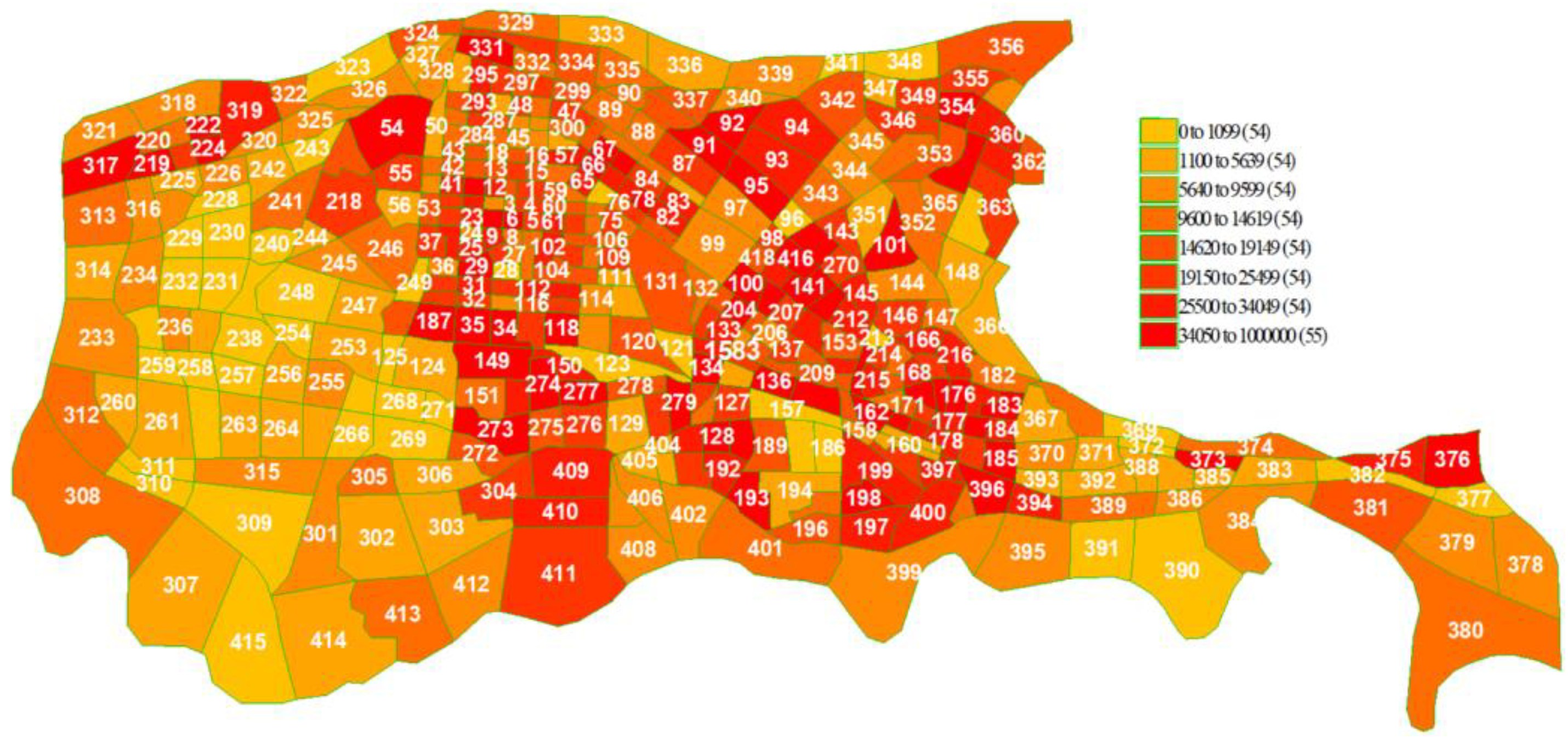
The trip intensity in the long-term planning year in the traffic zones is shown in Figure 18. According to the centroid coordinates of each traffic zone, the gravity center of urban trip intensity is calculated. The land-use intensity of the traffic zones in the long-term planning year is predicted, as shown in Figure 19. As we can see from Figure 18 and Figure 19, there is a strong correlation between the trip intensity and the land-use intensity in the traffic zones.

The city is divided into multiple circles centered at the gravity center ${\mathrm{O}}_{\mathrm{P}}$ by the radii with different lengths, and the difference in length between adjacent circles is 500 m. From Figure 19, we can see that the city does not develop evenly in all directions. Therefore, it is necessary to divide the city into different areas and calculate the fractal dimension of land-use intensity in each area separately. In this paper, the city is divided into four areas using four quadrants, as shown in Figure 20.

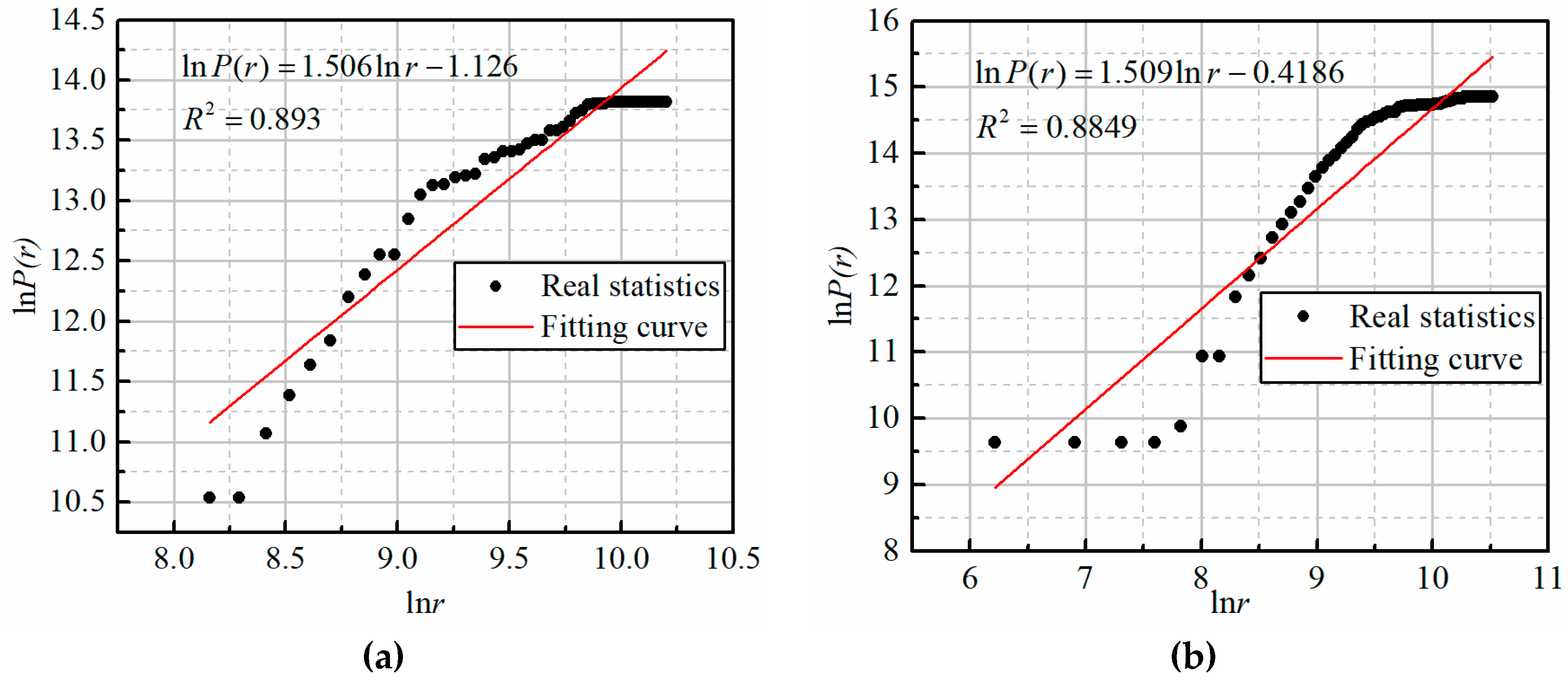
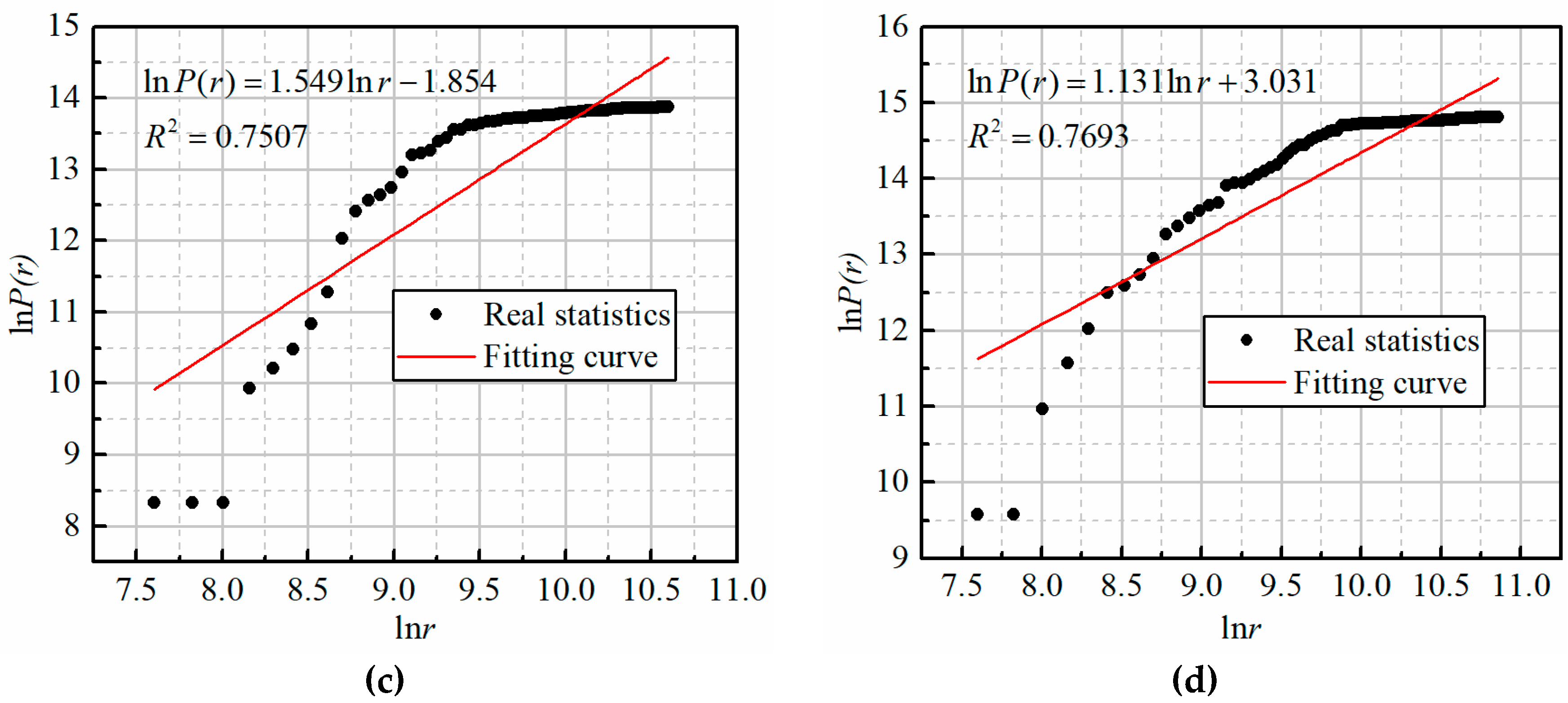
Taking logarithms on both sides of Equation (14), Equation (47) can be obtained. We can see that the fractal dimension $D_p$ can be got by linear regression.

$$\ln P(r)=D_p\ln r+a_0$$

(47)

where $a_0$ is a constant.

The double logarithmic relationships between land-use intensity and radii in the areas of four quadrants are recorded, and the fractal dimension of land-use intensity in each quadrant is obtained by regression fitting, as shown in Figure 21. As we can see from the fitting coefficients, the calculated fractal dimension vector of land-use intensity is $D_P=(1.506,1.509,1.549,1.131)$. The fractal dimensions are less than 2. So according to Equation (16), we can see that urban land-use intensity gradually decreases from the city center to the outside, and the decreasing trend of the area in the fourth quadrant is the fastest.

5.4. Results

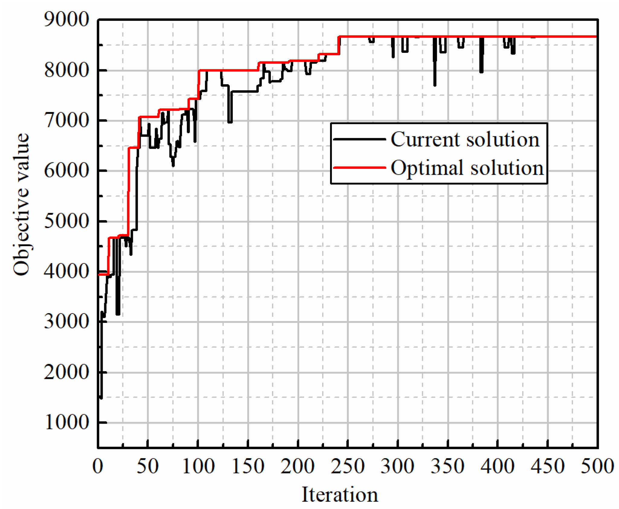
Based on the model and algorithm, the real-world case is calculated and the optimal solution in the existing iteration process (called optimal solution for short) is obtained. The optimal objective value Z is about 8664.2. The first objective value $Z_1$ is about 32,287 while the second objective value $Z_2$ is about 35,207. The iterative process of the algorithm is shown in Figure 22. As can be seen, the algorithm can converge quickly and has strong stability.

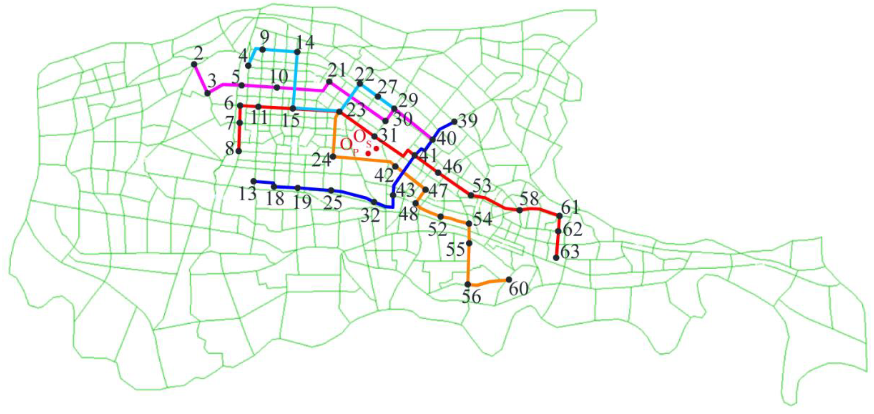
The optimal network is shown in Figure 23. The optimal network has 5 lines with a total length of 110.6 km, and the details of the lines is shown in

Table 5. Details of the lines in the optimal network.

Line	Sequence of stations in the line	Length
1	8–7–6–11–15–23–31–41–46–53–58–61–62–63	31.1 km
2	13–18–19–25–32–43–41–40–39	18.8 km
3	23–24–42–47–48–52–54–55–56–60	23.1 km
4	4–9–14–15–23–22–27–29	16.8 km
5	2–3–5–10–21–30–29–40	20.8 km

. The network presents the radial structure as a whole, and the central area is supplemented by a grid-like structure. The distance between the gravity center ${\mathrm{O}}_S$ of stations’ importance distribution and the gravity center ${\mathrm{O}}_{\mathrm{P}}$ of urban trip intensity is about 973.9 m, as shown in Figure 23. The matching degree $m_C$ between the optimal network and the urban trips is about 0.947, and the matching degree $m_F$ between the optimal network and the urban land use is about 0.893. In general, the network takes the east–west direction as the main axis, and the line alignments basically follow the routes covered by the main passenger flow corridors, which conforms to the banded development requirement of the city. The results showed that the layout of the network has a good match with the structure of the city.

6. Conclusions

In this paper, a quantitative model is developed to ensure that the generated urban rail transit network has a good match with urban road network, trips and land-use characteristics. The main contributions of the model are as follows:

• The basic network, which is determined according to the main locations of large traffic volume and main passenger flow corridors, is constructed to ensure matching between the network and the urban road network. With the basic network, the search range and the search direction of the line alignments can be bounded while generating the transit network.
• The matching index, which is calculated by the deviation value between two gravity centers of the stations’ importance distribution in the network and the traffic zones’ trip intensity, is proposed to constrain the matching degree between the network and the urban trip demand.
• Similarly, the matching index, which is calculated by the deviation value between the fractal dimensions of stations’ importance distribution and the traffic zones’ land-use intensity, is proposed to constrain the matching degree between the network and the land use.

To solve the model, a neighborhood search algorithm is developed based on the simulated annealing method. A real-size network is calculated with the model and algorithm. The generated network conforms to the development requirement of the city, which shows a good match between the network and the urban characteristics.

References

- Fielbaum, A.; Jara-Diaz, S.; Gschwender, A. A Parametric Description of Cities for the Normative Analysis of Transport Systems. Netw. Spat. Econ. 2017, 17, 343–365. [Google Scholar] [CrossRef]
- Fielbaum, A.; Jara-Diaz, S.; Gschwender, A. Optimal public transport networks for a general urban structure. Transp. Res. Part B Methodol. 2016, 94, 298–313. [Google Scholar] [CrossRef]
- Xiang, Z.; Waller, S.T.; Rey, D.; Duell, M. Integrating uncertainty considerations into multi-objective transportation network design projects accounting for environment disruption. Transp. Lett. Int. J. Transp. Res. 2019, 11, 351–361. [Google Scholar]
- Cadarso, L.; Codina, E.; Escudero, L.F.; Marín, A. Rapid transit network design: Considering recovery robustness and risk aversion measures. Transp. Res. Procedia 2017, 22, 255–264. [Google Scholar] [CrossRef]
- Canca, D.; De-Los-Santos, A.; Laporte, G.; Mesa, J.A. A general rapid network design, line planning and fleet investment integrated model. Ann. Oper. Res. 2014, 246, 127–144. [Google Scholar] [CrossRef]
- Gutiérrez-Jarpa, G.; Obreque, C.; Laporte, G.; Marianov, V. Rapid transit network design for optimal cost and origin–destination demand capture. Comput. Oper. Res. 2013, 40, 3000–3009. [Google Scholar] [CrossRef]
- Canca, D.; De-Los-Santos, A.; Laporte, G.; Mesa, J.A. An adaptive neighborhood search metaheuristic for the integrated railway rapid transit network design and line planning problem. Comput. Oper. Res. 2017, 78, 1–14. [Google Scholar] [CrossRef]
- Canca, D.; De-Los-Santos, A.; Laporte, G.; Mesa, J.A. Integrated Railway Rapid Transit Network Design and Line Planning problem with maximum profit. Transp. Res. Part E Logist. Transp. Rev. 2019, 127, 1–30. [Google Scholar] [CrossRef]
- Laporte, G.; Marin, A.; Mesa, J.A.; Perea, F. Designing robust rapid transit networks with alternative routes. J. Adv. Transp. 2011, 45, 54–65. [Google Scholar] [CrossRef] [Green Version]
- Cadarso, L.; Marín, Á. Improved rapid transit network design model: Considering transfer effects. Ann. Oper. Res. 2017, 258, 547–567. [Google Scholar] [CrossRef]
- Marín, Á.; García-Ródenas, R. Location of infrastructure in urban railway networks. Comput. Oper. Res. 2009, 36, 1461–1477. [Google Scholar] [CrossRef]
- Gallo, M.; Montella, B.; D’Acierno, L. The transit network design problem with elastic demand and internalisation of external costs: An application to rail frequency optimisation. Transp. Res. Part C Emerg. Technol. 2011, 19, 1276–1305. [Google Scholar] [CrossRef]
- López-Ramos, F.; Codina, E.; Marín, Á.; Guarnaschelli, A. Integrated approach to network design and frequency setting problem in railway rapid transit systems. Comput. Oper. Res. 2017, 80, 128–146. [Google Scholar] [CrossRef]
- Laporte, G.; Mesa, J.A. The design of rapid transit networks. In Location Science; Springer: Basel, Switzerland, 2015; pp. 581–594. [Google Scholar]
- Baum-Snow, N.; Kahn, M.E.; Voith, R. Effects of Urban Rail Transit Expansions: Evidence from Sixteen Cities, 1970–2000. Brook.-Whart. Pap. Urban Aff. 2005, 2005, 147–206. [Google Scholar] [CrossRef]
- Baum-Snow, N.; Kahn, M.E. The effects of new public projects to expand urban rail transit. J. Public Econ. 2000, 77, 241–263. [Google Scholar] [CrossRef]
- Dröes, M.I.; Rietveld, P. Rail-based public transport and urban spatial structure: The interplay between network design, congestion and urban form. Transp. Res. Part B 2015, 81, 421–439. [Google Scholar] [CrossRef]
- Laporte, G.; Mesa, J.A.; Perea, F. A game theoretic framework for the robust railway transit network design problem. Transp. Res. Part B Methodol. 2010, 44, 447–459. [Google Scholar] [CrossRef]
- Freeman, L.C. Centrality in social networks conceptual clarification. Soc. Netw. 1978, 1, 215–239. [Google Scholar] [CrossRef]
- Kourtellis, N.; Alahakoon, T.; Simha, R.; Iamnitchi, A.; Tripathi, R. Identifying high betweenness centrality nodes in large social networks. Soc. Netw. Anal. Min. 2013, 3, 899–914. [Google Scholar] [CrossRef]
- Mandelbrot, B. How long is the coast of britain? Statistical self-similarity and fractional dimension. Science 1967, 156, 636–638. [Google Scholar] [CrossRef]
- Benguigui, L.; Daoud, M. Is the suburban railway system a fractal? Geogr. Anal. 1991, 23, 362–368. [Google Scholar] [CrossRef]
- Levinson, D. Network structure and city size. PLoS ONE 2012, 7, e29721. [Google Scholar] [CrossRef] [PubMed]
Figure 1.
The gravity center of stations’ importance distribution.
Figure 2.
Urban rail transit lines in the city with radius .
Figure 3.
Urban rail transit lines laid along the main routes in the basic network.
Figure 4.
The gravity center of urban trip intensity.
Figure 5.
Deviation of the two gravity centers.
Figure 6.
The city is divided into four fan-shaped areas using four quadrants.
Figure 7.
The metro topological network in Beijing 2017 (288 stations).
Figure 8.
The relationship between the transfer times and the travel time in paths: (a) (insensitive to transfer); (b) , ; (c) , ; (d) , .
Figure 9.
The angle between adjacent sections in a line.
Figure 10.
Add a line randomly.
Figure 11.
Delete a line randomly.
Figure 12.
Add a section in a line randomly.
Figure 13.
Delete a section in a line randomly.
Figure 14.
Overall flow chart of the algorithm.
Figure 15.
Selected locations of large traffic volume in the urban central area.
Figure 16.
Urban passenger corridors in the urban central area.
Figure 17.
Basic network in the urban central area.
Figure 18.
The trip intensity in traffic zones.
Figure 19.
The land-use intensity in traffic zones.
Figure 20.
Division of urban circle layers and areas.
Figure 21.
Fractal fitting of land-use intensity in the areas within different quadrants: (a) within quadrant 1; (b) within quadrant 2; (c) within quadrant 3; (d) within quadrant 4.
Figure 22.
Process of iteration.
Figure 23.
The optimal network.