Spatial Analysis of Pottery Presence at the Former Pobedim Hillfort (an Archeological Site in Slovakia)


Abstract
:1. Introduction
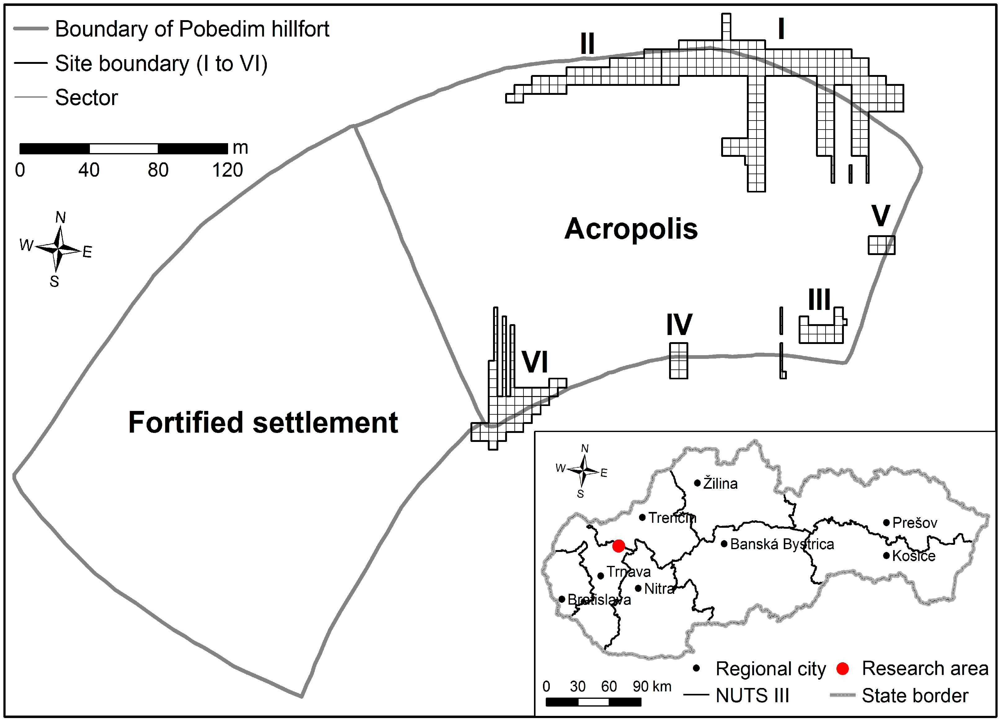
2. Research Area
3. Methods
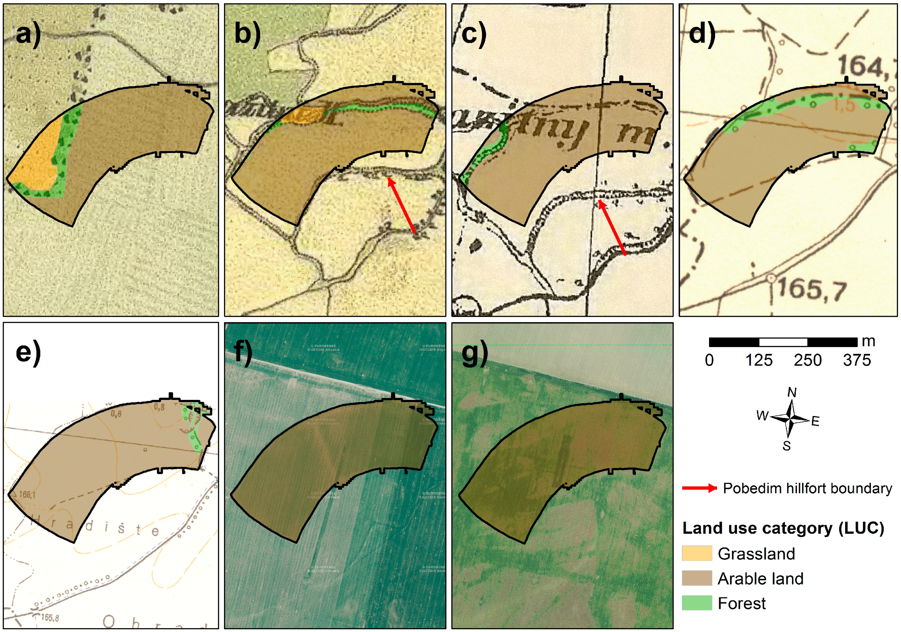
- (a)
- Map from the first military survey (years 1783–1785) at a scale 1:28,800,
- (b)
- Map from the second military survey (1845) at a scale of 1:28,800,
- (c)
- Reambulated map (1936) based on the map from the third military survey (1882) at a scale of 1:25,000,
- (d)
- Topographic map from 1956 at a scale of 1:25,000,
- (e)
- Topographic map from 1971 at a scale of 1:25,000,
- (f)
- Orthophotos from 2010 at a scale of 1:2000 and
- (g)
- Orthophotos from 2017 at a scale of 1:2000.
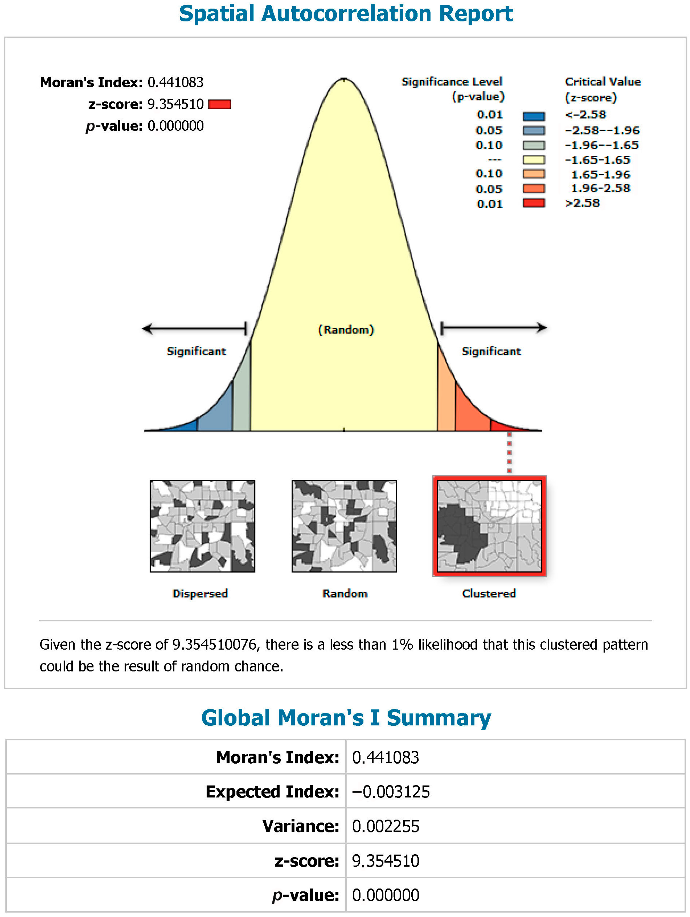
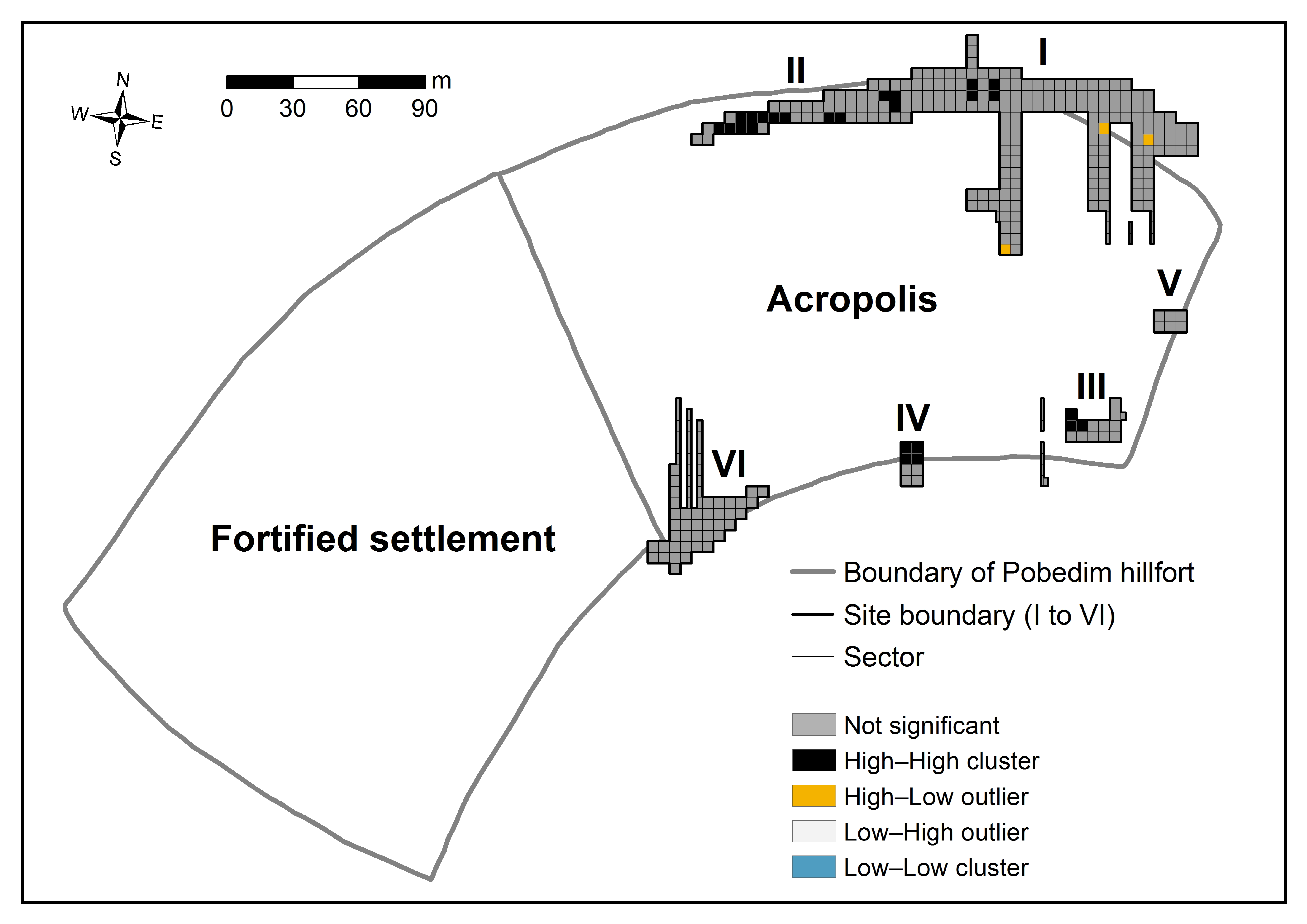
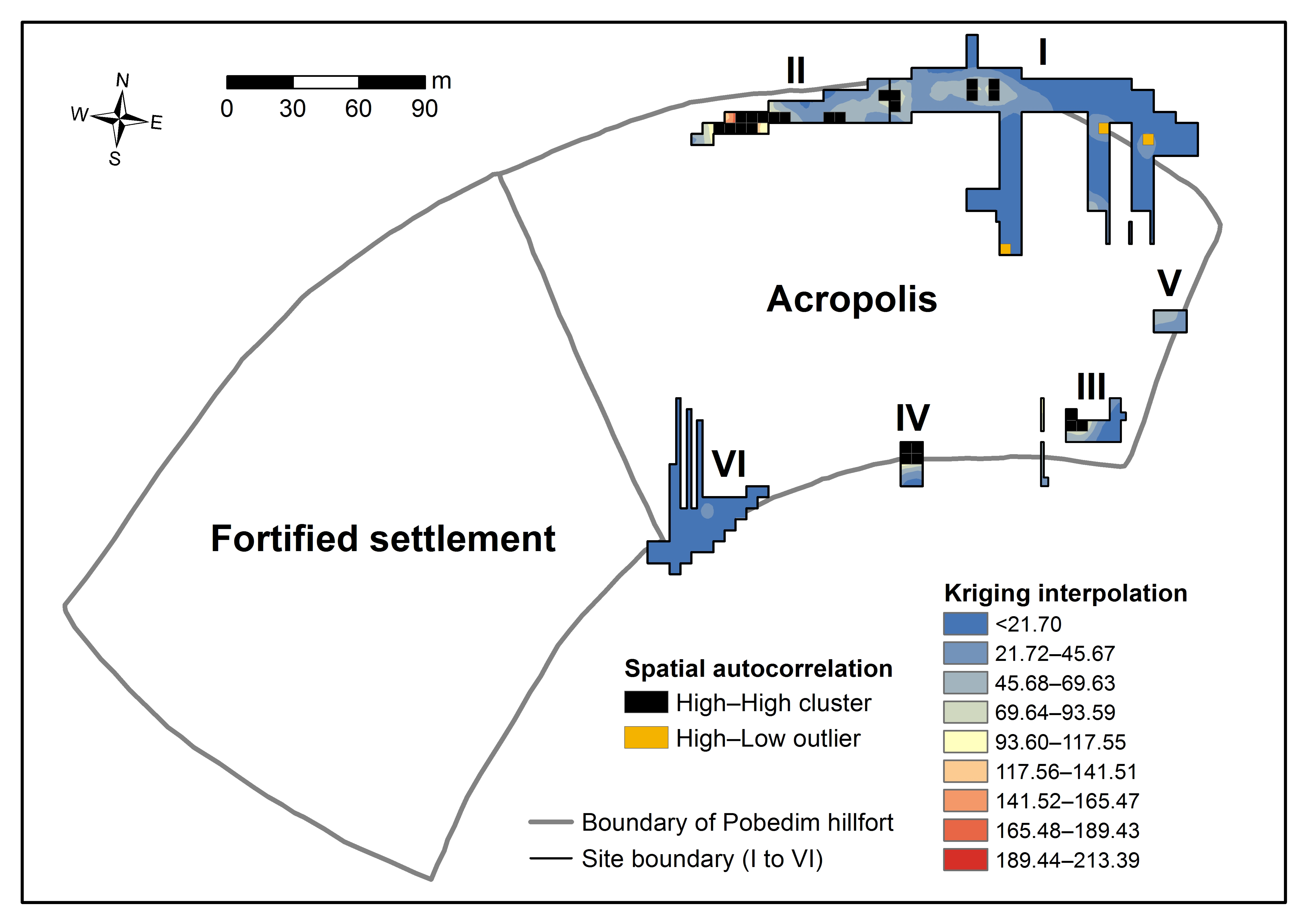
3.1. Spatial Autocorrelation
- (1)
- The LISA for each area (observation) indicates the extent of significant spatial clustering of similar values around this area.
- (2)
- The sum of LISA for all observations is proportional to the global indicator of spatial association.
- (1)
- Places with high values and similar neighbors: (high–high or H–H), known as hot spots, showing a scenario of positive spatial autocorrelation,
- (2)
- Places with low values and similar neighbors: (low–low or L–L), called cold spots, showing also a scenario of positive spatial autocorrelation,
- (3)
- Places with high values and neighbors with low values: (high–low or H–L), called potential spatial outliers, showing a negative spatial autocorrelation,
- (4)
- Places with low values and neighbors with high values: (low–high or L–H), again called spatial outliers, showing a negative spatial autocorrelation,
- (5)
- Places with no significant local spatial autocorrelation (not significant).
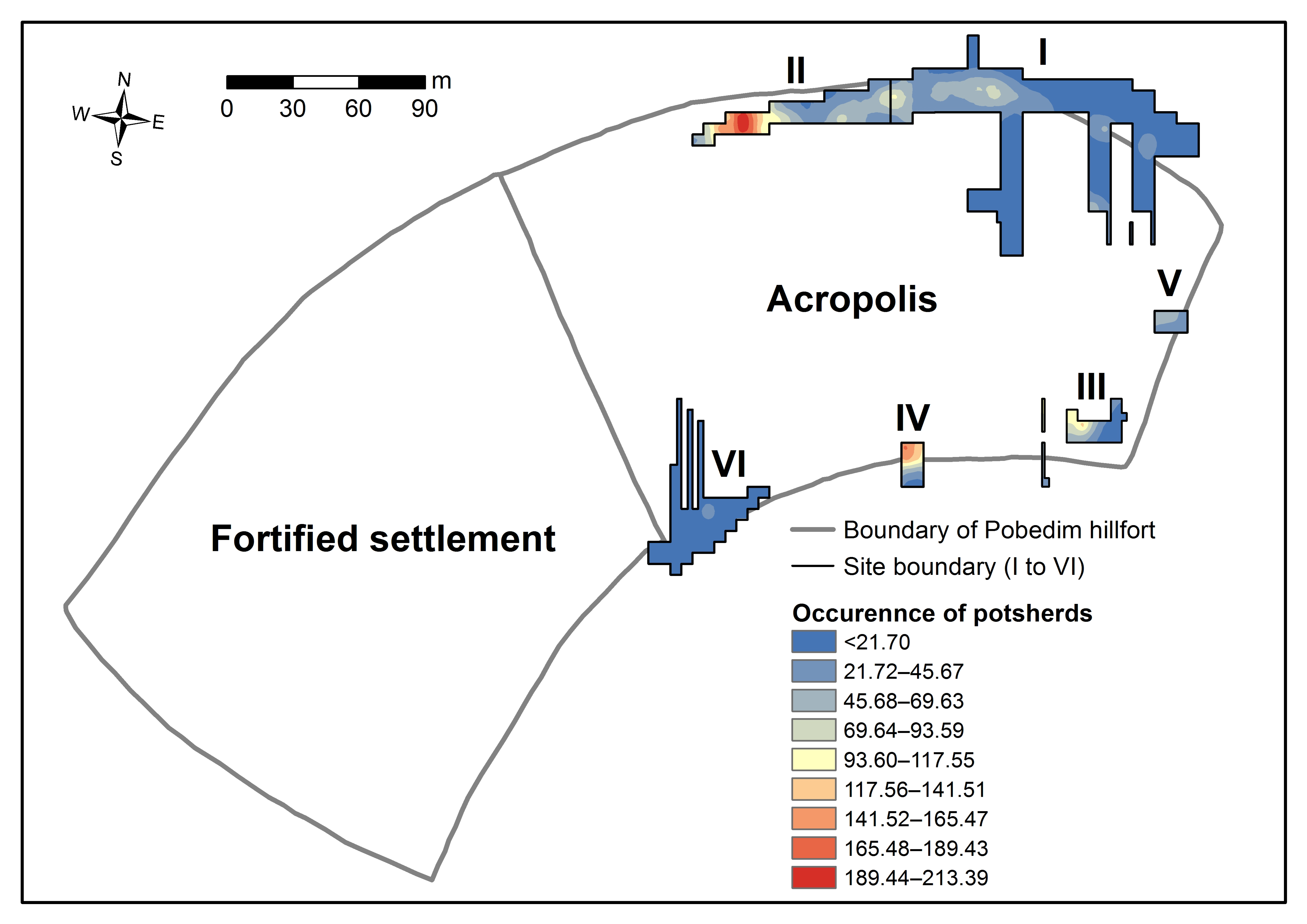
3.2. Kriging Interpolation
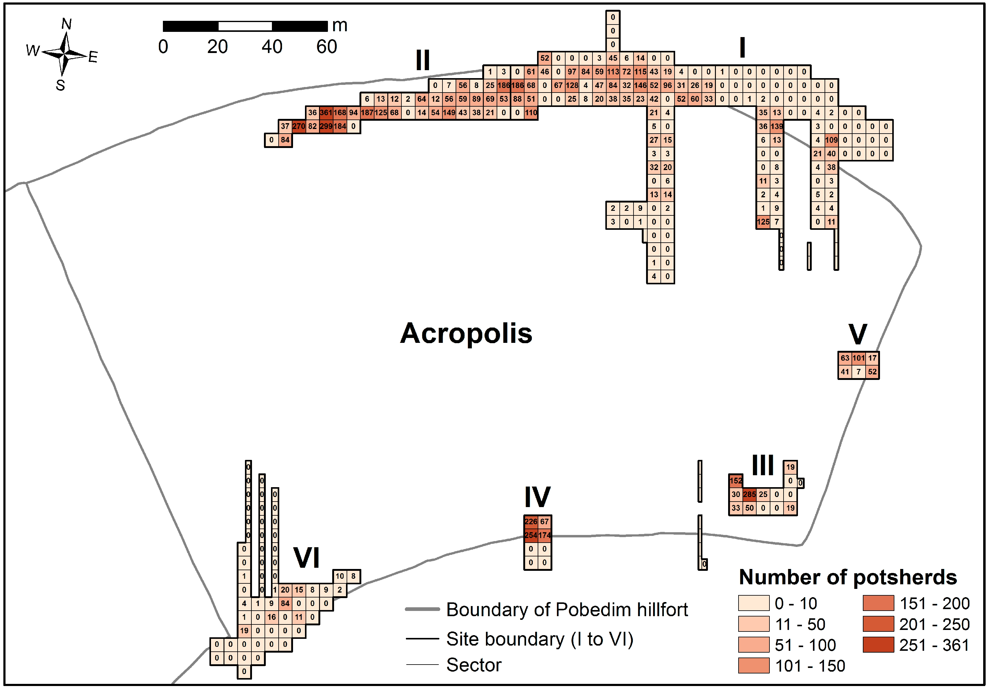
4. Results
5. Discussion
6. Conclusions
Author Contributions
Funding
Conflicts of Interest
References
- Stehlíková, B. Priestorová štatistika [Spatial Statistics]; SPU: Nitra, Slovakia, 2002. [Google Scholar]
- Tobler, W. A computer movie simulating urban growth in the Detroit region. Econ. Geogr. 1970, 46, 234–240. [Google Scholar] [CrossRef]
- Sun, X.; Luo, X.-S.; Xu, J.; Zhao, Z.; Chen, Y.; Wu, L.; Chen, Q.; Zhang, D. Spatio-temporal variations and factors of a provincial PM2.5 pollution in eastern China during 2013–2017 by geostatistics. Sci. Rep. 2019, 9, 3613. [Google Scholar] [CrossRef] [PubMed] [Green Version]
- Manjarrez-Domínguez, C.B.; Prieto-Amparán, J.A.; Valles-Aragón, M.C.; Delgado-Caballero, M.D.R.; Alarcón-Herrera, M.T.; Nevarez-Rodríguez, M.C.; Vázquez-Quintero, G.; Berzoza-Gaytan, C.A. Arsenic distribution assessment in a residential area polluted with mining residues. Int. J. Environ. Res. Public Health 2019, 16, 375. [Google Scholar] [CrossRef] [PubMed] [Green Version]
- Goovaerts, P. Geostatistics for Natural Resources Evaluation; Oxford University Press: New York, NY, USA, 1997. [Google Scholar]
- Webster, R.; Oliver, M.A. Geostatistics for Environmental Scientists, 2nd ed.; John Wiley &Sons: Chichester, UK, 2001. [Google Scholar]
- Dewar, G.; Marsh, E.J. the comings and goings of sheep and pottery in the coastal desert of Namaqualand, South Africa. J. Island Coast. Arch. 2019, 14, 17–45. [Google Scholar] [CrossRef]
- Harush, O.; Glauber, N.; Zoran, A.; Grosman, L. On quantifying and visualizing the potter’s personal style. J. Arch. Sci. 2019, 108, 104973. [Google Scholar] [CrossRef]
- VanValkenburgh, P.; Silva, L.O.G.; Repetti-Ludlow, C.; Gardner, J.; Crook, J.; Ballsun-Stanton, B. Mobilization as mediation implementing a tablet-based recording system for ceramic classification. Arch. Pract. 2018, 6, 342–356. [Google Scholar] [CrossRef]
- Pecci, A.; Dominguez-Bella, S.; Buonincontri, M.P.; Miriello, D.; de Luca, R.; di Pasquale, G.; Cottica, D.; Bernal-Casasola, D. Combining residue analysis of floors and ceramics for the study of activity areas at the Garum Shop at Pompeii. Arch. Anthrop. Sci. 2018, 10, 485–502. [Google Scholar] [CrossRef]
- Papworth, H.; Ford, A.; Welharn, K.; Thackray, D. Assessing 3D metric data of digital surface models for extracting archaeological data from archive stereo-aerial photographs. J. Arch. Sci. 2016, 72, 85–104. [Google Scholar] [CrossRef] [Green Version]
- Balla, A.; Pavlogeorgatos, G.; Tsiafakis, D.; Pavlidis, G. Efficient predictive modelling for archaeological research. Mediterr. Arch. Arch. 2014, 14, 119–129. [Google Scholar]
- Gümüş, M.G.; Durduran, S.S.; Bozdag, A.; Gümüş, K. GIS investigation of site selection of historical structures: The case of Knidos (Datça, Turkey). Mediterr. Arch. Arch. 2017, 17, 149–157. [Google Scholar]
- Balla, A.; Pavlogeorgatos, G.; Tsiafaki, D.; Pavlidis, D. Recent advances in archaeological predictive modeling for archeological research and cultural heritage management. Mediterr. Arch. Arch. 2014, 14, 143–153. [Google Scholar]
- Kaimaris, D. Ancient theaters in Greece and the contribution of geoinformatics to their macroscopic constructional features. Sci. Cult. 2018, 4, 9–25. [Google Scholar]
- Casas, L.; Tema, E. Investigating the expected archaeomagnetic dating precision in Europe: A temporal and spatial analysis based on the SCHA.DIF.3K geomagnetic field model. J. Arch. Sci. 2019, 108, 104972. [Google Scholar] [CrossRef]
- Niknami, K.A.; Amirkhiz, A.C.; Jalali, F. Spatial pattern of archaeological site distributions on the eastern shores of Lake Urmia, northwestern Iran. Archeol. Calc. 2009, 20, 261–276. [Google Scholar]
- Carrer, F. Interpreting intra-site spatial patterns in seasonal contexts: An ethnoarchaeological case study from the western alps. J. Arch. Method Theory 2017, 24, 303–327. [Google Scholar] [CrossRef] [Green Version]
- Gibbs, T. Descriptive spatial analysis of archaeological site distributions in the Kaibab National Forest, Arizona. In Proceedings of the 77th annual meeting of the Society for American Archaeology, Memphis, TN, USA, 18–22 April 2012; pp. 2–20. [Google Scholar]
- Lasaponara, R.; Masini, N. Facing the archaeological looting in Peru by using very high resolution satellite imagery and local spatial autocorrelation statistics. In Computational Science and Its Applications—ICCSA 2010; Taniar, D., Gervasi, O., Murgante, B., Pardede, E., Apduhan, B.O., Eds.; Springer: Berlin/Heidelberg, Germany, 2010; Volume 6016, pp. 254–261. [Google Scholar]
- Spurná, P. Prostorová autokorelace—všudypřítomný jev při analýze prostorových dat? [Spatial Autocorrelation—A Pervasive Phenomenon in the Analysis of Spatial Data?]. Czech Sociol. Rev. 2008, 44, 767–787. [Google Scholar]
- Bednárik, M.; Putiška, R.; Dostál, I.; Tornai, R.; Šilhán, K.; Holzer, F.; Weis, K.; Ružek, I. Multidisciplinary research of landslide at UNESCO site of Lower Hodruša mining water reservoir. Landslides 2018, 15, 1233–1251. [Google Scholar] [CrossRef]
- Weis, K.; Hronček, P. Using historic postcards and photographs for the research of historic landscape in geography and the possibilities of their digital processing. Eur. J. Geogr. 2017, 8, 77–85. [Google Scholar]
- Weis, K.; Kubinský, D. Analysis of changes in the volume of water in the Halčianske reservoir caused by erosion as a basis for watershed management. Geografie 2014, 119, 126–144. [Google Scholar]
- Kubinský, D.; Weis, K.; Fuska, J.; Lehotský, M.; Petrovič, F. Changes in retention characteristics of 9 historical artificial water reservoirs near Banská Štiavnica, Slovakia. Open Geosci. 2015, 7, 880–887. [Google Scholar]
- Ruttkay, M.; Hradištia, P. Veľkomoravské hradiská; Turčan, V., Ed.; Dajama: Bratislava, Slovakia, 2012. [Google Scholar]
- Bialeková, D. Pobedim v Praveku, Pobedim v Dobe Rímskej a v Dobe Sťahovania Národov, Pobedim v Dobe Slovanskej; SAV: Bratislava, Slovakia, 1992. [Google Scholar]
- Masný, M.; Zaušková, Ľ. Multi-temporal analysis of an agricultural landscape transformation and abandonment (Ľubietová, Central Slovakia). Open Geosci. 2015, 7, 888–896. [Google Scholar]
- Masný, M.; Weis, K.; Boltižiar, M. Case study area Ľubietová and Strelníky: Agricultural abandonment and land use changes since 1949. In Land Use/Cover Changes in Selected Regions in the World; IGU-LUCC Research Reports, Volume XIII; International Geographical Union Commission on Land Use and Land Cover Change: Asahikawa, Japan, 2018; pp. 43–51. [Google Scholar]
- Getis, A. A history of the concept of spatial autocorrelation: A geographer’s perspective. Geogr. Anal. 2008, 40, 297–309. [Google Scholar] [CrossRef]
- Gregory, D.; Johnston, R.; Pratt, G.; Watts, M.; Whatmore, S. The Dictionary of Human Geography, 5th ed.; Blackwell: Oxford, UK, 2009. [Google Scholar]
- Kusendová, D.; Solčianska, J. Testovanie priestorovej autokorelácie nezamestnanosti absolventov vysokých škôl okresov Slovenska [Testing of the spatial autocorrelation of unemployment of high schools graduates in the districts of Slovakia]. In Proceedings of the Sympózium GIS Ostrava 2007, Ostrava, Czechia, 28–31 January 2007. [Google Scholar]
- Hlásny, T. Geoštatistický koncept priestorovej závislosti pre geografické aplikácie [The geostatistical concept of spatial dependence for geographical applications]. Geogr. Časopis 2005, 57, 97–116. [Google Scholar]
- Griffith, D.A. Spatial Autocorrelation. A Primer; Association of American Geographers: Washington, DC, USA, 1987. [Google Scholar]
- Moran, P.A.P. Notes on continuous stochastic phenomena. Biometrika 1950, 37, 17–33. [Google Scholar] [CrossRef]
- Fotheringham, S.A.; Brunsdon, C.; Charlton, M. Geographically Weighted Regression—The Analysis of Spatially Varying Relationships; John Wiley & Sons: London, UK, 2002. [Google Scholar]
- Anselin, L. Local indicators of spatial association—LISA. Geogr. Anal. 1995, 27, 93–115. [Google Scholar] [CrossRef]
- Anselin, L. The Moran scatterplot as an ESDA tool to assess local instability in spatial association. In Spatial Analytical Perspectives on GIS in Environmental and Socio-Economic Sciences; Fischer, M., Ed.; Taylor and Francis: London, UK, 1996. [Google Scholar]
- Burrough, P.; McDonell, R. Principles of Geographical Information Systems; Oxford University Press: New York, NY, USA, 1998. [Google Scholar]
- Oliver, M.A. Kriging: A method of interpolation for geographical information systems. Int. J. Geogr. Inf. Syst. 1990, 4, 313–332. [Google Scholar] [CrossRef]
- Heine, G.W. A controlled study of some two-dimensional interpolation methods. COGS Comput. Contrib. 1986, 3, 60–72. [Google Scholar]
- McBratney, A.B.; Webster, R. Choosing functions for semi-variograms of soil properties and fitting them to sampling estimates. J. Soil Sci. 1986, 37, 617–639. [Google Scholar] [CrossRef]
- Kvamme, K.L. Spatial analysis and GIS: An integrated approach. In Computing the Past: Compute Applications and Quantitative Methods in Archaeology—CAA92; Andresen, J., Madsen, T., Scollar, I., Eds.; Aarhus University Press: Aarhus, Denmark, 1993. [Google Scholar]
- Zupancich, A.; Mutri, G.; Caricola, I.; Carra, M.L.; Radini, A.; Cristiani, E. The application of 3D modeling and spatial analysis in the study of groundstones used in wild plants processing. Arch. Anthrop. Sci. 2019, 11, 4801–4827. [Google Scholar] [CrossRef] [Green Version]
- Gennaro, A.; Candiano, A.; Fargione, G.; Mangiameli, M.; Mussumeci, G. Multispectral remote sensing for post-dictive analysis of archaeological remains. A case study from Bronte (Sicily). Arch. Prospect. 2019, in press. [Google Scholar] [CrossRef]
- Tache, A.V.; Sandu, I.C.A.; Popescu, O.C.; Petrisor, A.I. UAV solutions for the protection and management of cultural heritage. Case study: Halmyris archaeological site. Int. J. Conserv. Sci. 2018, 9, 795–804. [Google Scholar]
- Drap, P.; Papini, O.; Pruno, E.; Nucciotti, M.; Vannini, G. Ontology-based photogrammetry survey for medieval archaeology: Toward a 3D Geographic Information System (GIS). Geosciences 2017, 7, 93. [Google Scholar] [CrossRef] [Green Version]
- Lieskovský, J.; Kaim, D.; Balázs, P.; Boltižiar, M.; Chmiel, M.; Grabska, E.; Király, G.; Konkoly-Gyuró, E.; Kozak, J.; Antalová, K.; et al. Historical land use dataset of the Carpathian region (1819–1980). J. Maps 2018, 14, 644–651. [Google Scholar] [CrossRef] [Green Version]
- Munteanu, C.; Kuemmerle, T.; Boltižiar, M.; Lieskovský, J.; Mojses, M.; Kaim, D.; Konkoly-Gyuro, E.; Mackovčin, P.; Müller, D.; Ostapowicz, K.; et al. Nineteenth-century land-use legacies affect contemporary land abandonment in the Carpathians. Reg. Environ. Chang. 2017, 11, 2209–2222. [Google Scholar] [CrossRef]
- Zhao, K.L.; Fu, W.J.; Qiu, Q.Z.; Ye, Z.Q.; Li, Y.F.; Tunney, H.; Dou, C.Y.; Zhou, K.N.; Qian, X.B. Spatial patterns of potentially hazardous metals in paddy soils in a typical electrical waste dismantling area and their pollution characteristics. Geoderma 2019, 337, 453–462. [Google Scholar] [CrossRef]
- Miri, M.; Alahabadi, A.; Ehrampush, M.H.; Rad, A.; Lotfi, M.H.; Sheikhha, M.H.; Sakhvidi, M.J.Z. Mortality and morbidity due to exposure to ambient particulate matter. Ecotoxicol. Environ. Saf. 2018, 165, 307–313. [Google Scholar] [CrossRef]
- Dai, W.; Zhao, K.L.; Fu, W.J.; Jiang, P.K.; Li, Y.F.; Zhang, C.S.; Gielen, G.; Gong, X.; Li, Y.H.; Wang, H.L.; et al. Spatial variation of organic carbon density in topsoils of a typical subtropical forest, southeastern China. Catena 2018, 167, 181–189. [Google Scholar] [CrossRef]
- Shahid, S.U.; Iqbal, J.; Hasnain, G. Groundwater quality assessment and its correlation with gastroenteritis using GIS: A case study of Rawal Town, Rawalpindi, Pakistan. Environ. Monitor. Assess. 2014, 186, 7525–7537. [Google Scholar] [CrossRef]
- Nakoinz, O.; Knitter, D. Modelling Human Behaviour in Landscapes; Springer International Publishing: Basel, Switzerland, 2016. [Google Scholar]
- Hengl, T. A Practical Guide to Geostatistical Mapping of Environmental Variables; Office for Official Publications of the European Communities: Luxembourg, 2007. [Google Scholar]
- Olea, R.A. Geostatistics for Engineers and Earth Scientists; Kluwer Academic Publishers: New York, NY, USA, 1999. [Google Scholar]
- Wackernagel, A. Multivariate Geostatistics; Springer-Verlag: Berlin, Germany, 1995. [Google Scholar]


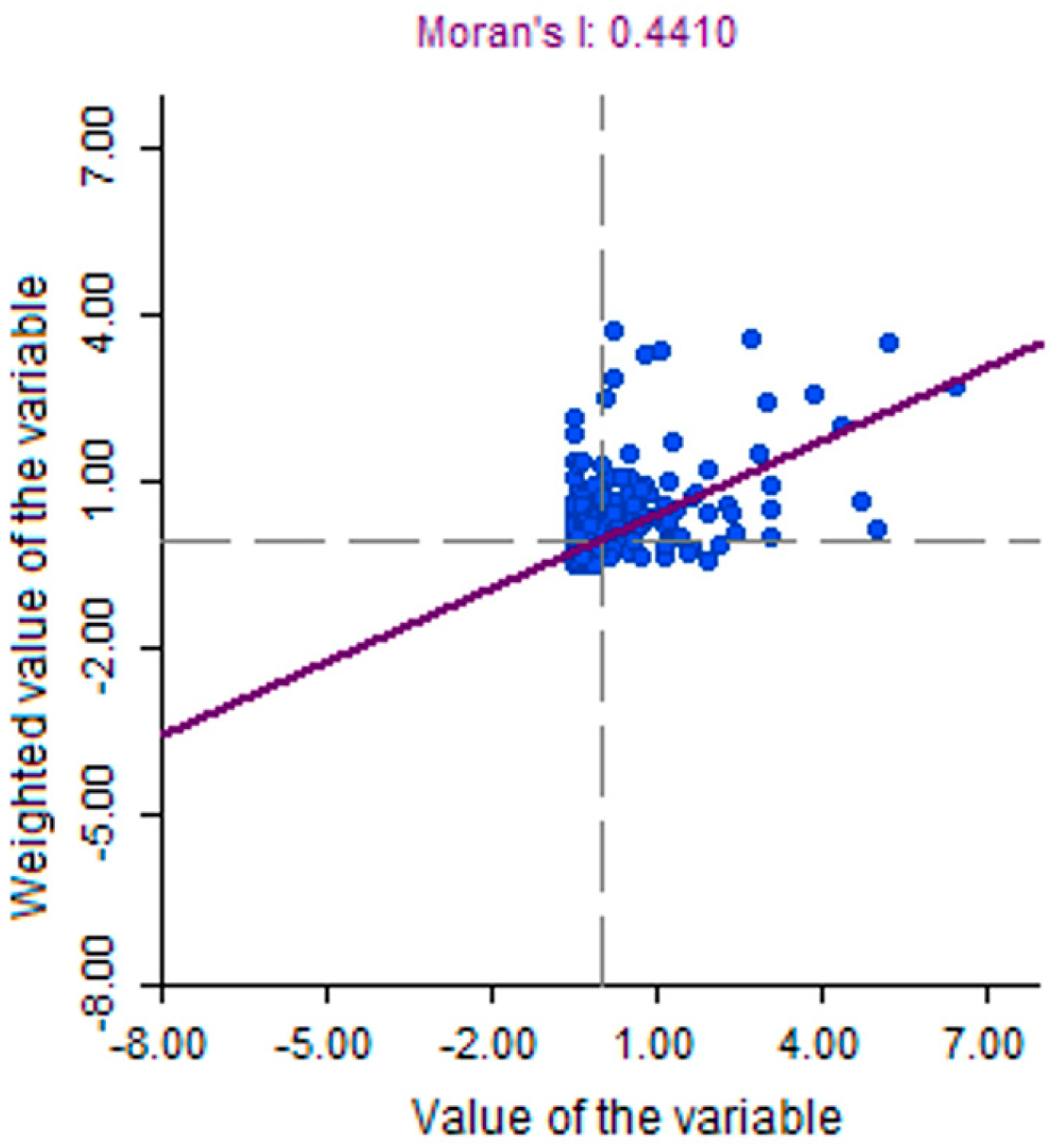
| Variable | Moran Coefficient | p-Value | z-Score Value |
|---|---|---|---|
| Potsherds (number) | 0.4410 | 0.0000 * | 9.3545 |
© 2019 by the authors. Licensee MDPI, Basel, Switzerland. This article is an open access article distributed under the terms and conditions of the Creative Commons Attribution (CC BY) license (http://creativecommons.org/licenses/by/4.0/).
Share and Cite
Vojteková, J.; Vojtek, M.; Tirpáková, A.; Vlkolinská, I. Spatial Analysis of Pottery Presence at the Former Pobedim Hillfort (an Archeological Site in Slovakia). Sustainability 2019, 11, 6873. https://0-doi-org.brum.beds.ac.uk/10.3390/su11236873
Vojteková J, Vojtek M, Tirpáková A, Vlkolinská I. Spatial Analysis of Pottery Presence at the Former Pobedim Hillfort (an Archeological Site in Slovakia). Sustainability. 2019; 11(23):6873. https://0-doi-org.brum.beds.ac.uk/10.3390/su11236873
Chicago/Turabian StyleVojteková, Jana, Matej Vojtek, Anna Tirpáková, and Ivona Vlkolinská. 2019. "Spatial Analysis of Pottery Presence at the Former Pobedim Hillfort (an Archeological Site in Slovakia)" Sustainability 11, no. 23: 6873. https://0-doi-org.brum.beds.ac.uk/10.3390/su11236873