Application of Non-Parametric Bootstrap Confidence Intervals for Evaluation of the Expected Value of the Droplet Stain Diameter Following the Spraying Process

Abstract

In the era of sustainable agriculture, the issue of proper and precise implementation of agrotechnical operations, without harmful effects on the natural environment, begins to play an important role. Statistical tools also become important, for example, when assessing the malfunction of plant cultivation equipment. The study presents a comparison of six nonparametric bootstrap methods used for construction of confidence intervals for the expected value of an average diameter of droplet stains following the spraying process. The simulation tests were carried out based on experiment with nozzle sprayer Lechler 110-03 using two spray nozzles: a new one and an old one. It was assumed that the distribution of the droplet stain size was consistent with the lognormal distribution. The paper considers the influence of the sample size, mean value and standard deviation of the droplet stain diameter on the interval range as well as on the estimated coverage probabilities of the confidence intervals. It was shown that in general these methods can be applied for this purpose. For the double bootstrap method and the studentized method, the empirical confidence levels of the constructed intervals turned out to be less distinct than the assumed level but the lengths of these intervals were greater than the lengths of intervals obtained using the other four methods.

1. Introduction

Sustainable agriculture aims to promote a sustainable farming system that relies on the rational use of natural resources, which allows reducing the negative impact of agriculture on the environment and prevents the loss of organic matter in the soil. It is part of a larger movement towards sustainable development, which suggests that natural resources are limited, recognizes the constraints of economic growth and encourages equality in resource allocation. Sustainable agricultural development has been proposed as one of the alternatives to reverse the spiral of resource degradation and poverty. The goal of sustainable agriculture is to protect natural resources [1,2]. Sustainable development is one of the principles on which the European Union (EU) policy should be based, including the EU’s common agricultural policy. The common agricultural policy is the main institutional structure and the main factor of reforms affecting the development of sustainable agriculture [3].

Spraying is the basic and the most widely used treatment in plant protection but improperly preformed or defective technical equipment may degrade the quality of agricultural raw materials and pose a threat to humans and the environment. Recently, plant protection has been severely criticized for creating environmental and human hazards. The use of pesticides, in addition to unquestionable effectiveness, has serious disadvantages. Creation of resistant biotypes, which are difficult to combat later, can be another possible threat. In addition, chemicals change crop biochemistry, pollute the environment and often destroy natural enemies who would limit the host population [4].

However, the use of herbicides, despite many controversies, is one of the basic methods of protecting plants against weeds in modern agriculture. The use of plant protection products (generally known as pesticides or agrochemicals) makes it possible to increase food production by destroying weeds and pests that attack crops. As a result, productivity per hectare increases and also reduces losses during transport and storage of food [5]. In addition, the use of pesticides gives the farmer the opportunity to intervene quickly when the crop is directly threatened by diseases and pests. This is especially important in the case of mass and sudden outbreaks of pests. Some chemicals, for example, seed mortars, have a preventive effect. In turn, granulated pesticides introduced into the soil and taken up by plant roots operate for the whole period or a significant part of the growing season [6].

The effect of herbicides depends on both the technical and technological processes that make up the spraying procedure, as well as the behaviour of the active substance on the sprayed surface of the plants and inside them. These processes include the production of spray liquid droplets (atomization), transfer from the atomizer to the plant surface, droplet retention on plants, formation of sediments on the leaf surface after evaporation of water from the spray liquid, up-taking of the active substance (absorption) and its translocation and metabolism [7].

A number of technological, technical and climatic factors influence the quality of the sprayer work. The most important of them include the type of machine, choice of nozzles, spray parameters, temperature and humidity as well as compliance with the instructions of producers of plant agents [8]. It should be noted that the nozzle wear degree has a decisive influence on spray quality. Application of excessive numbers of droplets on the protected surface causes their merging, which worsens the quality of spraying. Gravity makes droplets on the surface of plants penetrate the soil and reach groundwater [5,9]. Besides, if nozzles generate very small droplets, they are drifted away by wind or the liquid evaporates before falling on protected plants.

In spraying operations, it is important that as much of the spray liquid as possible settles on the surface of the plant. This is the basic condition for achieving high effectiveness of the procedure, as well as reducing losses that burden the environment. Liquid settlement on plants depends mainly on the development phase of the plant, crop density, dose, type of usable liquid and operation of the spraying apparatus [10]. It was stated that in the total spray liquid expenditure balance (during wheat spraying) 52.4% were losses in the air (as a result of drift and evaporation) and as a result of falling on the soil, while 47.6% sprayed liquid stopped on the plants [11]. These are significant losses that can cause environmental pollution.

A uniform distribution of the spray liquid has a significant influence on the environmental impact of agrochemicals. Uneven application means that a more larger dose of the agent is applied over a large field area than it results from actual needs. It is not only a waste but it also carries the risk of the accumulation of residues of plant protection agents in agricultural raw materials [12].

For these reasons, statistical analysis of the droplet stains after the spraying process is important for adjustment of the operating parameters of the sprayer. One of the statistical methods that can be used is the analysis of the droplet stain distribution, especially point or interval estimation of the parameters of their distribution. Naturally occurring droplets are usually irregular in shape and different in size. This resulted in the introduction of different mean droplet diameter definitions along with statistical description of the droplet size distribution (linear, surface and volume (Sauter)).

The conducted research regarding the estimation of droplet size and quantity involves the division into raindrops and droplets following the spraying process, where various types of probability distribution can be applied to describe each of the two cases presented above. As regards empirical data obtained for raindrops, the following distributions are used most frequently—exponential [13], gamma [14,15,16], Gauss [17], lognormal [18,19], Weibull [20,21] and Poisson [22]. The gamma distribution is used to describe the droplet size distribution following the spraying process [23]. Equivalently, the following distributions are also used for the same type of data—upper truncated lognormal [24,25], Rosin–Rammler and Nukiyama–Tanasawa [26] and Weibull [18,27]. The lognormal distributions with the upper truncation [15,23] are applicable for the distribution of droplet diameters because the measured droplet diameters are in a certain interval ranging from zero to a definite upper limit, which in an extreme case can be a maximum measured droplet size.

A number of parametric and non-parametric methods have been designed for interval estimation of the expected value of a random variable with a lognormal distribution. A few such procedures were described and compared in Reference [28], including the Cox method for a large sample size presented in Reference [29], a conservative method described in Reference [30] and a parametric bootstrap method [31]. Based on numerical results, it was demonstrated [28] that all these procedures, with the exception of the Cox method, are too conservative or too liberal disregarding the sample size. Therefore, the methods of construction confidence intervals presented above are not satisfactory for small sample sizes. This problem was solved in Reference [32], where the method was developed for construction of exact confidence intervals for small sample sizes using the idea of a generalized p-value and generalized confidence intervals.

The bootstrap method was designed by Bradley Efron [23,24,26,33]. The group of bootstrap methods includes parametric and non-parametric methods, including inter alia—the basic, percentile, bias-corrected, bias-corrected and accelerated, studentized and double bootstrap methods. These methods differ as regards the selection of appropriate quantiles of the distribution of the estimators from bootstrap samples. Bootstrap is a relatively new method but in the computer era it is frequently used for obtaining confidence intervals and test hypotheses in situations when the sample sizes are small, the distribution of estimators is unknown or when the fulfilment of relevant assumptions is doubtful. The statistical research carried out in Reference [27], showed that the information on the asymmetry of the probability distribution of a random variable or initial estimation of the asymmetry coefficient can be helpful while determining the sample size both in bootstrap tests and classical significance tests.

The aim of this study was to investigating the possibility of using various bootstrap methods to generate confidence intervals to assess the average droplet trace diameter, which can be characterized by an asymmetric probability distribution set close to the lognormal one. The simulations were limited to the ranges of droplet trace sizes obtained in experimental experiments using the Lechler 110-03 sprayer. The usefulness of particular methods is indicated depending on the size of the random sample and the different degree of variability of the obtained droplet trace sizes. The tests carried out are aimed at determining the methods of assessing the degree of wear of the sprayer nozzle.

2. Materials and Methods

2.1. Material

The analysis carried out in the research concerns the estimation of the mean value of droplet stain diameters following the spraying process carried out in an experimental study on a Lechler 110-03 spray nozzle type. The nominal flow rate for this type of the spray nozzle is 1.17 $\mathrm{L}·{\min }^{-1}$. The spray boom shift during spraying was 9 $\mathrm{km}·{\mathrm{h}}^{-1}$ (2.5 $\mathrm{m}·{\mathrm{s}}^{-1}$) and the pressure was 5 bar (0.5 MPa). After the droplets applied on each piece of foil dried, scans of 5 × 5 cm images were obtained. The scanner resolution during scanning was 300 dpi. The size of droplet stains and the number of droplets was calculated using the computer software Image Pro+ by Media Cybernetics. The new spray nozzle and older one were examined for comparison in a research experiment. The older nozzle was obtained as a result of laboratory wearing using Kaolin KOM water slime from SURMIN-KAOLIN. The slime was produced by adding 9.1 kg of kaolin to 150 L of water [34]. After reaching 10% wearing, the liquid outflow rate was measured at 1.29 $\mathrm{L}·{\min }^{-1}$. In Figure 1 examples of scans obtained from the spraying process using new spray nozzle (a) and older one (b) are shown.

2.2. Mathematical Background

The density function $f\left(x\right)$ of the lognormal distribution for the diameter size of the splashed droplets following the spraying process is given by:

$$f\left(x\right)=\frac{1}{x\sigma \sqrt{2\pi }}exp\left(-\frac{{(log\left(x\right)-\mu )}^2}{2{\sigma }^2}\right),$$

(1)

where:

$x\in (0,+\infty )$ – droplet diameter [$\mathsf{\mu }$m],

$\mu \in <0,+\infty )$ – expected value of variable ln(X), location parameter,

$\sigma >0$ – standard deviation, scale parameter,

$log(·)$ – natural logarithm.

$Y=log\left(X\right)\sim N(\mu ,\sigma )$.

The parameters of the lognormal distribution turn out to be the functions of both parameters $\mu$ and ${\sigma }^2$ and this dependence poses difficulties in obtaining exact and optimal tests and confidence intervals. In particular, the expected value of lognormal random variable X depends on $\mu$ and ${\sigma }^2$:

$$E\left(X\right)=E\left(exp\left(Y\right)\right)=exp\left(\mu +\frac{1}{2}{\sigma }^2\right).$$

(2)

The overlapping of droplet stains following the spraying process is an additional difficulty in using these stains to estimate the distribution of the spraying parameters. The poor accuracy in point estimation of the mean value and standard deviation has an impact on the interval estimation of these parameters. Taking into account the above difficulties, six non-parametric bootstrap methods were used to construct the confidence intervals—basic, percentile, bias-corrected, bias-corrected and accelerated, studentized and double bootstrap methods.

During the research work, the sensitivity of the lengths and coverage of intervals constructed using the discussed bootstrap methods were compared, given the changes in the sample sizes and changes in the values of standard deviation. The consistency of empirical coverages was also compared with the assumed confidence level.

Let $\mathbf{x}=(x_1,x_2,\dots ,x_n)$ denote an n-element random sample, whereas $R(x,F)$ is some statistics determined on the sample space with distribution F, $\theta$ is the unknown parameter and $\sigma$ is the standard deviation of this parameter. The bootstrap sample is an n-element realization of the variable X, ${\mathbf{x}}^{*}=(x_1^{*},x_2^{*},\dots ,x_n^{*})$ and its elements are selected at random with replacement from sample x. In order to obtain bootstrap samples, independent B-fold $\left(B\ge 1000\right)$ generation of n-element data sequences ${\mathbf{x}}^{*}=(x_1^{*},x_2^{*},\dots ,x_n^{*})$ is carried out. These data sequences are used to determine the estimator $\widehat{\theta }$ of the $\theta$ parameter. As a result, B-element sequence of estimators ${\widehat{\theta }}_j^{*}=R\left(x_j^{*}\right)$, $j=1,2,\dots ,n$ is obtained. Out of the sequence of estimators ${\widehat{\theta }}_j^{*}$, the quantiles of a fixed rank are calculated, which are then used to obtain the confidence interval for parameter $\theta =R\left(x\right)$.

In the simplest basic method (B), the $(1-\alpha )$% confidence interval for parameter $\theta$ is obtained according to the formula:

$$\left(2\widehat{\theta }-{\widehat{\theta }}_{\left(1-\frac{\alpha }{2}\right)}^{*},2\widehat{\theta }-{\widehat{\theta }}_{\left(\frac{\alpha }{2}\right)}^{*}\right),$$

(3)

where:

${\widehat{\theta }}_{\left(\alpha \right)}^{*}$ denotes ${\alpha }^{th}$ quantile from the sequence of values ${\widehat{\theta }}_j^{*}$,

$\widehat{\theta }$ denotes the estimator from the original sample $\mathbf{x}=(x_1,x_2,\dots ,x_n)$.

The percentile (P), bias-corrected (BC) and bias-corrected and accelerated (BCa) methods confidence intervals do not use estimator $\widehat{\theta }$ but are calculated exclusively based on quantiles of a relevant rank from the sequence of estimators:

$$\left({\widehat{\theta }}_{\left({\alpha }_L\right)}^{*},{\widehat{\theta }}_{\left({\alpha }_U\right)}^{*}\right),$$

(4)

where the ranks ${\alpha }_L$ and ${\alpha }_U$ of appropriate percentiles can be calculated according obtained sequence of estimators ${\widehat{\theta }}_j^{*}=R\left(x_j^{*}\right)$, $j=1,2,\dots ,n$ depending on selected method.

The bootstrap method with bias correction [35] contributes to improvement of the precision of the percentile method in the case when the median of estimator values for all bootstrap samples is not equal to the value of the estimator for the original sample. This method adds two steps after estimation of the distribution of the considered parameter for bootstrap samples:

-

calculation of the fraction k of bootstrap samples for which the estimator value of the parameter is lower than the estimator calculated on the basis of the original sample,

-

calculation of interval bounds regarding the calculated fraction of samples in order to correct the bias.

Similar to the previous method, the bias-corrected and accelerated bootstrap method (BCa) [24,35] takes into account the fact that estimators of the parameter for bootstrap samples can be biased and the impact of individual values in a sample on the value of the estimator is considered as well. When the distribution is skewed, some adjustment needs to be made and BCa method gives such a possibility.

The ranks ${\alpha }_L$ and ${\alpha }_U$ of percentiles in BCa method depend on two constants a and $z_0$ called the acceleration and bias correction coefficient. The standard error of $\widehat{\theta }$ is stabilized by coefficient a and $z_0$ measures the median bias of ${\widehat{\theta }}^{*}$. This results in faster convergence of the estimator confidence limit into its exact value than in the case of the quantile method. Thus, the probability of coverage for the BCa method is closer to the nominal probability than in the percentile method.

There are different ways to determine the value of coefficient a. One of them uses the jackknife method [24], which explores the impact of n individual elements of a sample by using n special sample size $n-1$. Each of the n new samples is obtained through deleting each time only one element from the original sample. Based on such samples, n estimators of the $\theta$ parameter are calculated.

In the studentized method, sometimes referred to as the bootstrap-t method, the appropriate statistic quantiles are used in the following form:

$$t^{*}=\frac{{\widehat{\theta }}^{*}-\widehat{\theta }}{\widehat{\sigma }\left({\widehat{\theta }}^{*}\right)},$$

(5)

where $\widehat{\sigma }\left({\widehat{\theta }}^{*}\right)$ is the estimator of the standard error of the estimator ${\widehat{\theta }}^{*}$ determined based on the bootstrap sample $x^{*}=(x_1^{*},x_2^{*},\dots ,x_n^{*})$.

The double bootstrap method is a modification of the previous method [36], where the standard error $\sigma \left({\widehat{\theta }}^{*}\right)$ of ${\widehat{\theta }}^{*}$ is estimated on bases of additional $B_1$ bootstrap samples ${\mathbf{x}}^{**}=(x_1^{**},x_2^{**},\dots ,x_n^{**})$ generated from the ${\mathbf{x}}^{*}$ sample, where ${\overline{\theta }}^{**}=\frac{1}{B_1}{\sum }_{i=1}^{B_1}{\widehat{\theta }}_i^{**}$.

This section outlines the six bootstrap methods, which were used in this study. More details and appropriate mathematical formulas of individual methods can be found in numerous studies available in the cited literature.

2.3. Computer Simulations

On the basis of the experimental tests, the ranges of the average diameters of droplet traces obtained in the spraying process using the tested nozzles were estimated. The determined ranges of means as well as standard deviations obtained for the droplet stains were used as the basis for conducting computer simulations using the six bootstrap methods described in the previous section. The simulations were carried out taking into account different sample sizes (10–600 elements). For each combination of two values of the analyzed mean and standard deviation, ten thousand samples were generated consisting of equal elements each, which were used for generating bootstrap samples. For each random sample x, the total of $B=2000$ bootstrap samples were generated, based on which the relevant percentiles were estimated. In the case of a double bootstrap, the standard deviation was estimated based on $B_1=250$ samples. For each generated sample, all six types of confidence intervals were calculated and the assumed confidence level was $\alpha =0.05$. Computer simulations were carried out using software MATLAB R2014a by employing our own code and embedded procedures on the computer with the operating system Windows 10 Professional equipped with an Intel Xeon E5-2609 2.40 GHz processor.

3. Results

The analysis took into account the mean values and standard deviation values estimated on the basis of the measurements performed with the Lechler 110-03 sprayer. The first step involved testing the consistency of the distribution of size of droplets stain diameters from the measurements with the lognormal distribution and determining its parameters.

The considered sample scans, which were previously presented on Figure 1, resulted in a highly asymmetrical distribution of droplet stain diameters. The distribution of droplet diameters obtained while spraying using a new and old nozzle are presented in

Table 1. Droplet traces size distribution in an example datasets.

Stain Class	No. Objects	% Objects	% Area	Diameter Mean	Diameter Std
New nozzle
<150 $\mathsf{\mu }$m	511	62.01	43.96	123.89	19.19
150–250 $\mathsf{\mu }$m	242	29.37	36.72	184.29	22.61
250–350 $\mathsf{\mu }$m	61	7.40	15.95	293.17	52.33
350–450 $\mathsf{\mu }$m	9	1.09	3.17	382.51	69.80
>450 $\mathsf{\mu }$m	1	0.12	0.19	471.00	0.00
Older nozzle
<150 $\mathsf{\mu }$m	323	51.43	37.49	132.34	14.37
150–250 $\mathsf{\mu }$m	204	32.48	35.71	196.42	15.69
250–350 $\mathsf{\mu }$m	80	12.74	19.09	295.28	24.28
350–450 $\mathsf{\mu }$m	12	1.91	3.69	412.07	39.19
>450 $\mathsf{\mu }$m	9	1.43	4.01	521.74	47.16

. The drops traces were divided into 5 size classes—0–150$\mathsf{\mu }$m, 150–250$\mathsf{\mu }$m, 250–350$\mathsf{\mu }$m, 350–450$\mathsf{\mu }$m and above $450\mathsf{\mu }$m. The estimates were obtained using computer software Image Pro+ by Media Cybernetics. The table includes the number of objects assigned to classes, the percentage of objects, the percentage of surface covered and the average drop values and standard deviations in each class. The data compiled in Table 1 show a strongly asymmetrical distribution.

In addition, to determine the approximate parameters of the droplet size distribution, a division into a larger number of size classes was made (Figure 2). For both nozzles (new and old), using the MatLab function fitnlm, parameters of log-normal distribution were determined, which are best fitted to the obtained histograms for selected droplet size classes. For the new nozzle, the average is ${\mu }_x=160.3\mathsf{\mu }$m and the standard deviation ${\sigma }_x=65.8\mathsf{\mu }$m, while for the older nozzle the average is ${\mu }_x=186.7\mathsf{\mu }$m and the standard deviation ${\sigma }_x=81.2\mathsf{\mu }$m.

Due to the overlapping of droplet stains following the spraying process and the difficulties in construction of the confidence intervals for the expected value of the lognormal distribution, we chose the bootstrap methods [24]. As already mentioned, the confidence intervals, constructed using the discussed bootstrap methods were compared in terms of the sensitivity of their lengths and probabilities of the expected value coverage to changes in sample sizes and in values of standard deviation. The consistency of empirical coverage probabilities with the assumed confidence level was also compared.

The analysis took into account the mean values and standard deviation values estimated based on the measurements performed with the Lechler 110-03 sprayer. In order to generate samples from the lognormal distribution for the population mean, the range from $90\mathsf{\mu }$m to $210\mathsf{\mu }$m was taken with a step of ten units, whereas for the standard deviation the range was from $30\mathsf{\mu }$m to $180\mathsf{\mu }$m with a step of ten units. For each combination of two values of the analyzed mean and standard deviation, ten thousand samples were generated consisting of thirty elements each, which were random samples used for generating bootstrap samples. For each random sample x, the total of $B=2000$ bootstrap samples were generated, based on which the relevant percentiles were estimated. In the case of a double bootstrap, the standard deviation was estimated based on $B_1=250$ samples. The values of B and $B_1$ were determined according to Reference [36]. For each generated sample, all six types of confidence intervals were calculated and the assumed confidence level was $\alpha =0.05$.

The largest differences between the results obtained by different methods occurred for small samples. Figure 3 presents numerical results of the coverage of the calculated confidence intervals for the assumed 95% confidence levels using the six bootstrap methods with division to the selected lengths of the mean value and standard deviation value $({\mu }_x,{\sigma }_x)$ of variable X. In a majority of cases, all the considered methods give the coverage probabilities lower than the assumed level of 95% for sample sizes of 30. The confidence intervals constructed with the studentized and double bootstrap methods give the coverage probabilities not greater than 94% for each considered value of the mean; noteworthy, the variation of the feature may be high and, in a particular case, the variation coefficient may even be equal to 80%. The other four methods allow obtaining coverage probabilities not greater than 93%; however, only for the variation coefficient not higher than 34% (Figure 3).

In order to study the impact of the sample size on the lengths of confidence intervals for the examined bootstrap methods, the sample sizes considered in the simulations were 10, 20, 30, 50, 80, 100, 150, 200, 400 and 600. Since the interval lengths for larger sample sizes overlap, the figure presents only the lengths for the smaller sample sizes (up to 100 elements). The samples were generated from a population for which the mean value was 160 $\mathsf{\mu }$m and the standard deviation ranged from 40 to 120 $\mathsf{\mu }$m. For each of the sizes, five thousand samples were generated and the length of the confidence interval calculated with the six studied methods was estimated based on each sample. The lengths of the intervals obtained were averaged for each method separately. From the graph presented in Figure 4 (for the standard deviation of 80 $\mathsf{\mu }$m, close to the sample obtained from the experiment), it is evident that the intervals for the studentized and double bootstrap methods are wider, compared with the basic, percentile, bias correction and accelerated methods. Concurrently, it can be noted that the lengths of the confidence intervals for the four methods mentioned above are fairly equal (Figure 4).

The four methods—namely, basic, percentile, bias correction and accelerated methods—give intervals characterized by similar length but different from the results obtained using the studentized and double bootstrap methods, which are mutually comparable (Hall, 1992). Hence, the graph shows the comparison of the lengths of the confidence intervals only for two methods—the percentile and double bootstrap methods (Figure 4). For small sample sizes and large standard deviation, the lengths of the intervals obtained using the double bootstrap method are even approximately 3 times longer than those obtained using the percentile method. For larger sample sizes, these differences are less visible.

In the study of the influence of the sample size on the coverage probabilities of confidence intervals, obtained in particular for the smaller sample sizes, the follwing sample sizes were included in the simulation—10, 20, 30, 50, 80, 100, 150, 200, 400 and 600 (Figure 5). For each sample size, five thousand samples were generated from the same population as previously (mean value $160\mathsf{\mu }$m and standard deviation from 40 to $120\mathsf{\mu }$m) and the percentage of covering of the assumed value of 160 was checked.

The intervals obtained using the analyzed methods give a similar covering of the true value of the population mean only for samples with a size of at least 100–200 elements. For smaller sample sizes, we obtained a clear division of the discussed methods into three groups. Given the interval lenghts discussed above, the covering is closest to the assumed confidence level for the studentized and double bootstrap intervals, followed by the bias correction, percentile, accelerated and basic methods. According to the considered criterion, the worst covering is provided by the basic method (Figure 6).

The graph presented in Figure 7 and

Table 2. Coverage probabilities of the expected value by confidence intervals constructed using nonparametric bootstrap methods depending the sample size and different values of standard deviation, ${\mu }_x=160\mathsf{\mu }$m.

Sample Size	Standard Deviation	B	P	BC	BCa	S	D
10	40	0.897	0.897	0.895	0.895	0.947	0.946
	80	0.843	0.859	0.861	0.865	0.932	0.932
	120	0.789	0.821	0.828	0.847	0.921	0.922
20	40	0.918	0.919	0.919	0.917	0.946	0.948
	80	0.881	0.895	0.899	0.901	0.937	0.938
	120	0.838	0.864	0.870	0.882	0.924	0.924
30	40	0.928	0.932	0.933	0.934	0.950	0.949
	80	0.898	0.911	0.913	0.917	0.941	0.942
	120	0.869	0.892	0.897	0.905	0.934	0.934
50	40	0.935	0.935	0.936	0.939	0.947	0.947
	80	0.919	0.925	0.926	0.928	0.943	0.944
	120	0.883	0.902	0.907	0.914	0.932	0.933
80	40	0.944	0.945	0.946	0.946	0.950	0.952
	80	0.925	0.934	0.935	0.931	0.942	0.944
	120	0.895	0.907	0.908	0.910	0.926	0.925
100	40	0.943	0.940	0.941	0.941	0.944	0.945
	80	0.930	0.938	0.937	0.935	0.944	0.944
	120	0.905	0.917	0.919	0.920	0.934	0.936
150	40	0.948	0.949	0.948	0.948	0.952	0.953
	80	0.931	0.937	0.937	0.937	0.942	0.943
	120	0.921	0.930	0.932	0.932	0.942	0.943
200	40	0.941	0.941	0.940	0.941	0.945	0.946
	80	0.943	0.946	0.947	0.946	0.950	0.951
	120	0.928	0.939	0.941	0.939	0.948	0.949
400	40	0.947	0.946	0.946	0.945	0.947	0.947
	80	0.942	0.946	0.946	0.946	0.946	0.948
	120	0.936	0.940	0.939	0.941	0.944	0.946
600	40	0.949	0.951	0.949	0.949	0.952	0.952
	80	0.946	0.946	0.946	0.946	0.948	0.949
	120	0.940	0.942	0.941	0.939	0.942	0.944

show the influence of the standard deviation on the coverage of confidence intervals. As in the case of the comparison of the interval lengths, the graph shows a comparison of only the percentile method and the double bootstrap method (Figure 7, Table 2). The difference between the coverages of the intervals obtained using these methods are visible mainly for small sample sizes.

4. Discussion

Agricultural ecosystems have been designed to provide food, fibre and fuel. Ecosystem services such as nutrient recirculation, pollination and water flow are often referred to as endangered resources in modern societies. Agricultural systems can therefore be seen as heterogeneous but nested socio-ecological systems requiring an institutional environment [3].

Man-made climate change has created major challenges to achieve sustainable agriculture by depleting ecological and natural resources. Existing climate change has an impact on water resources. Some countries are already experiencing severe water scarcity or are reaching their limits [37]. The most promising strategy for achieving sustainable development is to replace hazardous agrochemicals with environmentally friendly preparations from symbiotic microorganisms that could provide protection against biotic and abiotic substances [38].

The main conflict in the pursuit of sustainable development is between economic maximization of growth and environmental protection [39]. On a global scale, agriculture is one of the main sources of degradation of ecosystem services. Also in Europe, most of today’s agriculture has a severe negative impact on ecosystems, for example contributing to global carbon cycle disorders, loss of biodiversity and increasing eutrophication. The transition to more sustainable agriculture is necessary to avoid further degradation of ecosystems [3]. The presented assessments of various authors regarding the impact of pesticide use on the natural environment, agricultural production and human health indicate that an important element is proper plant protection technique and compliance with spraying parameters. These parameters can have a significant impact on the quality of the plant protection treatment and the state of the environment.

To reduce the harmful effects of plant protection agents on the environment, we should aim to reduce herbicide doses. In Reference [40], authors based on their own research, say that the dose can be reduced from 12.5% to 50%. In their view, this does not significantly reduce crop yield, while maintaining the required herbicidal effectiveness. The use of herbicides in reduced doses brings the best results in spring cereals, because weeds in these crops are in the early stages of development and thus are easier to eliminate. Very good results can be obtained in plantations with low weed intensity and in the case of controlling species sensitive to a given herbicide. The weaker effect of reduced doses is obtained in winter cereals and especially barley. This fact is caused by the fact that weeds are more advanced in development. Producers of plant protection products are also trying to reduce the content of the active substance, contributing to the reduction of production costs and demonstrating their concern for the state of the environment [8].

Another way to protect the environment is to reduce the number of treatments through the combined use of agrochemicals. Appropriate mixtures of plant protection products give the possibility of wider protection of cereals and affect the increase of yields. The effectiveness of mixtures often does not differ from the effectiveness of preparations used separately and in some cases is even greater. It should be remembered that only well-tested and tested combinations of preparations can be used together [41].

It was therefore considered that it would be more reasonable to systematically implement an integrated model for controlling harmful organisms than to use only chemical methods. The idea of sustainable development combines economic growth with environmental protection and the global balance of ecosystems. According to this concept, the increase in agricultural production can only occur through the increase of resource productivity and thus the introduction of technologies that simultaneously protect resources and maintain their high quality for future generations. The need to develop environmentally friendly agriculture is increasingly accepted in Poland. An important element of it is the change of some agrotechnical methods due to the need to protect ground and surface waters. Restricting the use of chemicals is justified because they cause a number of negative effects [42]—they contribute to the emergence of pesticide-resistant breeds of pests, diseases and weeds, destroy beneficial organisms by reducing their numbers and can even lead to their complete elimination from ecosystems, reduce the value of the environment by contaminating soil, surface and groundwater, lead to a decrease in the nutritional value of plant and animal products as a result of persistence of their residues or metabolites, negatively affect human health.

Ensuring the quality of spraying is a key process in plant protection, which is to ensure high yields while minimizing the adverse impact on the environment [43]. Proper spraying of field crops is influenced by many factors that can be grouped into three categories—1. Equipment and techniques used; 2. Spray quality. 3. Operator skills [44]. All leading atomizer manufacturers offer “low-drift” nozzles that produce droplets less prone to drift [44]. Currently produced atomizers and in particular Venturi nozzles, are designed to produce larger diameter droplets. These designs were created because droplets with a smaller diameter (<$200\mathsf{\mu }$m) are more likely to drift [45]. The quality of the plant protection treatment is influenced by the height of the boom position above the sprayed surface [45].

One of the methods used for improvement of the properties of liquids used for plant protection is usage of adjuvants. They improve spraying efficiency by equalizing droplet size and reducing wind drift. They reduce the level of the surface tension of liquid, so they enable coverage more surface of the leaf blade and at the same time they increase absorbing properties of plants. An additional benefit of adjuvants is availability of combining various types of plant protection agents and their use during one treatment [46].

According to Directive 2009/128/EC of the European Parliament establishing a framework for the sustainable use of pesticides, ways to reduce the impact of pesticides on the environment are determined and thus also maintaining the safety of field crops. Particularly great importance is attached to the precise use of pesticides on protected plants. An important issue is the application of the pesticide in such a way that it is effective in use and at the same time safe for the environment. The safety of pesticide use in agriculture depends on the techniques used. At present, great importance is attached to eliminating drift of liquid used during plant protection treatment. The quality of the plant protection treatment depends, among others on atomizer type, working pressure and working speed. The type of atomizer used and the operating pressure determine the droplet size produced by the atomizer. Sprayers wear out during operation and the parameters of their work change. These changes are expressed by the increase in the flow rate of the liquid as well as the spectrum of droplets produced (VMD) [46].

The research topics discussed in the papers make it important to determine the most precise determination of the distribution of droplets generated by sprayers. Because the statistical probability distribution for droplet trace diameters is not fully specified, as presented in the introduction, computer methods become helpful when analysing these problems. Their example are the bootstrap methods, which allows, for example, to generate confidence intervals for a specific parameter or statistics. As the simulation studies show, they do not always give the right results. Results are influenced by among others size of the random sample or too large variability of the examined feature. However, simulation studies have shown that under certain conditions, these methods give reliable results and allow the study properties of variables with asymmetrical statistical distributions, which is confirmed by Reference [27].

Despite some advantages, bootstrap confidence intervals may be heavily distorted and therefore may be misleading. This problem is especially noticeable for simple bootstrap methods and small samples. This is confirmed by the results of other authors who also received inaccurate estimates of confidence intervals in their studies [47]. In addition, bootstrap methods are time consuming, and not always more complex methods give better results, and significantly increase the cost of calculations [48]. Despite these drawbacks, bootstrap methods are a powerful tool for creating confidence intervals. They do not need sophisticated mathematical models and are often used in the absence of information about statistical distributions of the studied features. In addition, for samples of over 200 elements, all examined bootstrap methods give similar results, so in such cases the percentile method seems sufficient. It is the least time-consuming than other more advanced bootstrap methods. For smaller samples studentized and double bootstrap gives more proper estimates.

The applied method of assessing the size of sprayed droplets obtained from sprayers by means of measuring the size of traces left on the surface is burdened with a certain error. Some drops fall in the same place or close to each other, as a result of which some traces are enlarged compared to real ones. For larger drops, the most commonly left traces do not have a circular shape, which causes additional inaccuracies in the estimation of the size of traces left by the computer image analysis program. However, this method, apart from determining the droplet size distribution, also allows the surface coverage of falling drops to be assessed.

In future research, the authors intend to focus on further analysis of spray droplet distribution using more accurate droplet size measurement methods (using in-flight laser measurement). Additionally, the use of the bootstrap method to estimate other parameters of the droplet size distribution obtained from the sprayer will allow for a more precise assessment of sprayer nozzle wear and unevenness of the generated droplets.

5. Conclusions

The comparison of the empirical probabilities of coverage of the expected value by the examined six bootstrap confidence intervals used for estimation of the mean droplet stain diameter following the spraying process performed with the Lechler 110-03 sprayer nozzle leads to the following conclusions:

-

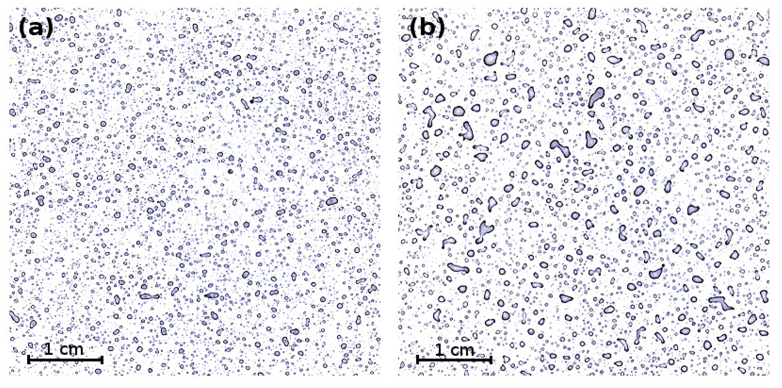
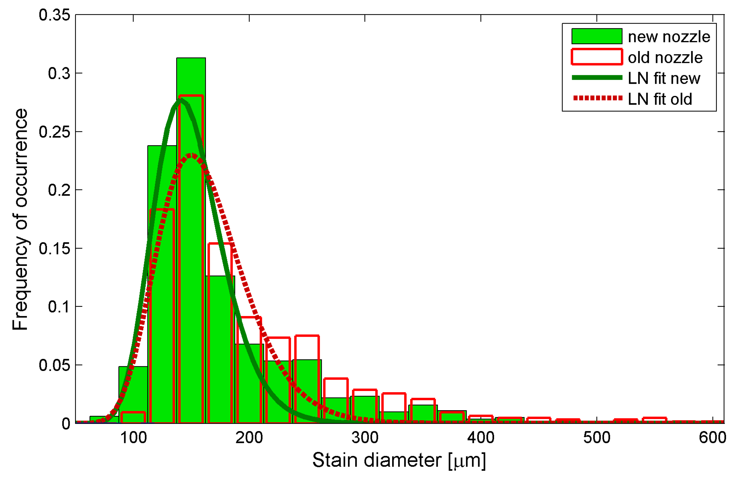
The size distribution of traces of droplets obtained from sprayers is asymmetrical, similar to the log-normal distribution.

-

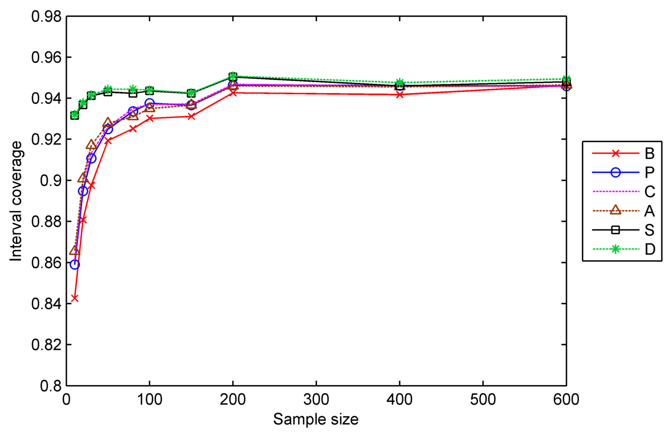
The six bootstrap methods compared give confidence intervals that in general do not hold the assumed confidence level especially for small samples.

-

The bootstrap methods are generally useful for constructing confidence intervals for the expected value of droplet diameter but not all methods always give confidence intervals that in general hold the assumed confidence level.

-

The simulation studies conducted here can be used in practice with the interval estimation of the expected value of droplet stain diameters. An adequate method should be selected depending on the sample size, in particular in the case of smaller sizes (below 100) and depending on the variability of data.

-

The studentized and double bootstrap methods allow obtaining less distinct coverage than the assumed confidence level, compared with the other four methods.

-

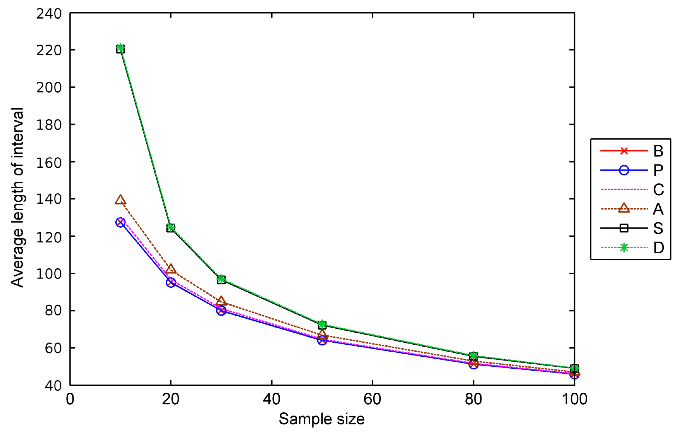
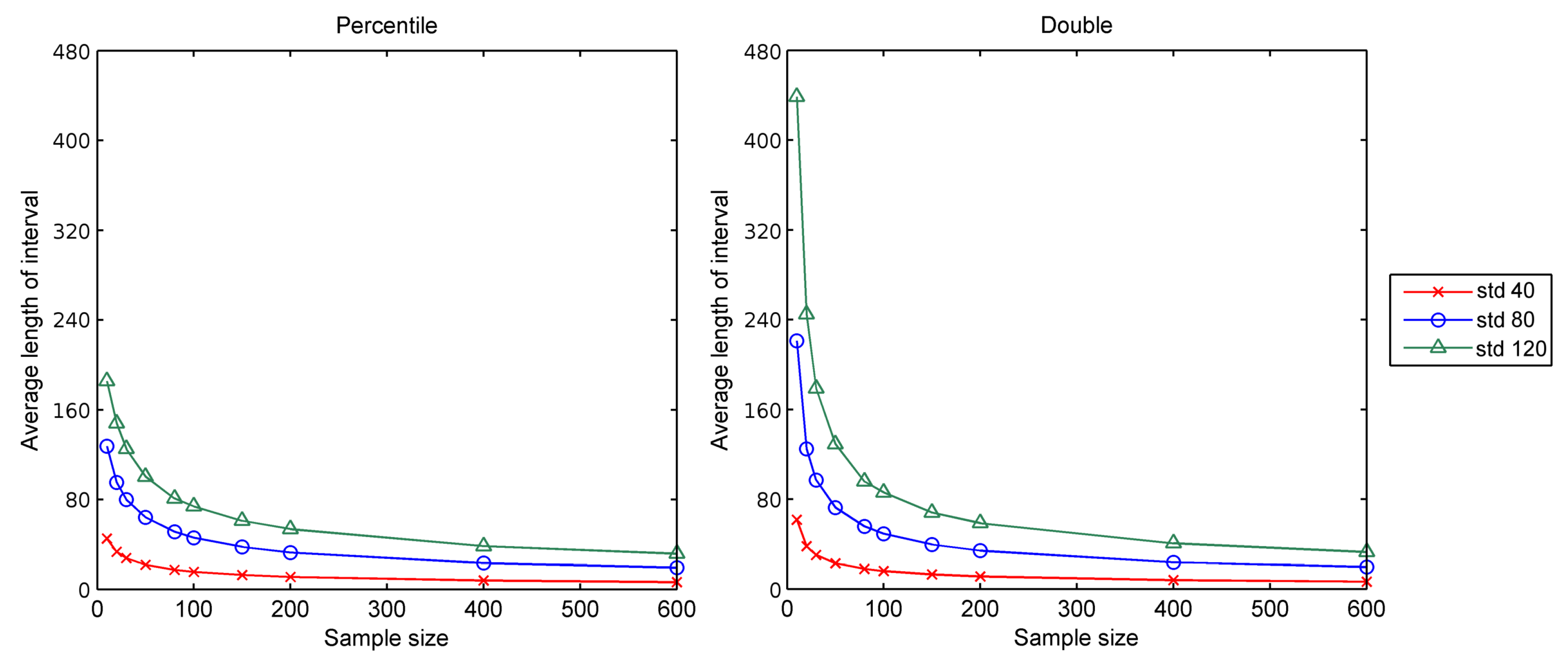
For small sample sizes, the lengths of the confidence intervals obtained using the studentized and double bootstrap methods are similar, greater than the intervals from the other four methods.

-

Although the confidence intervals obtained by the studentized and double bootstrap methods maintain the assumed coverage level, however, for small samples the estimated confidence intervals are too wide, which makes it impossible to use them in practice. It is recommended to use samples with at least 100-200 elements for usefull confidence intervals.

-

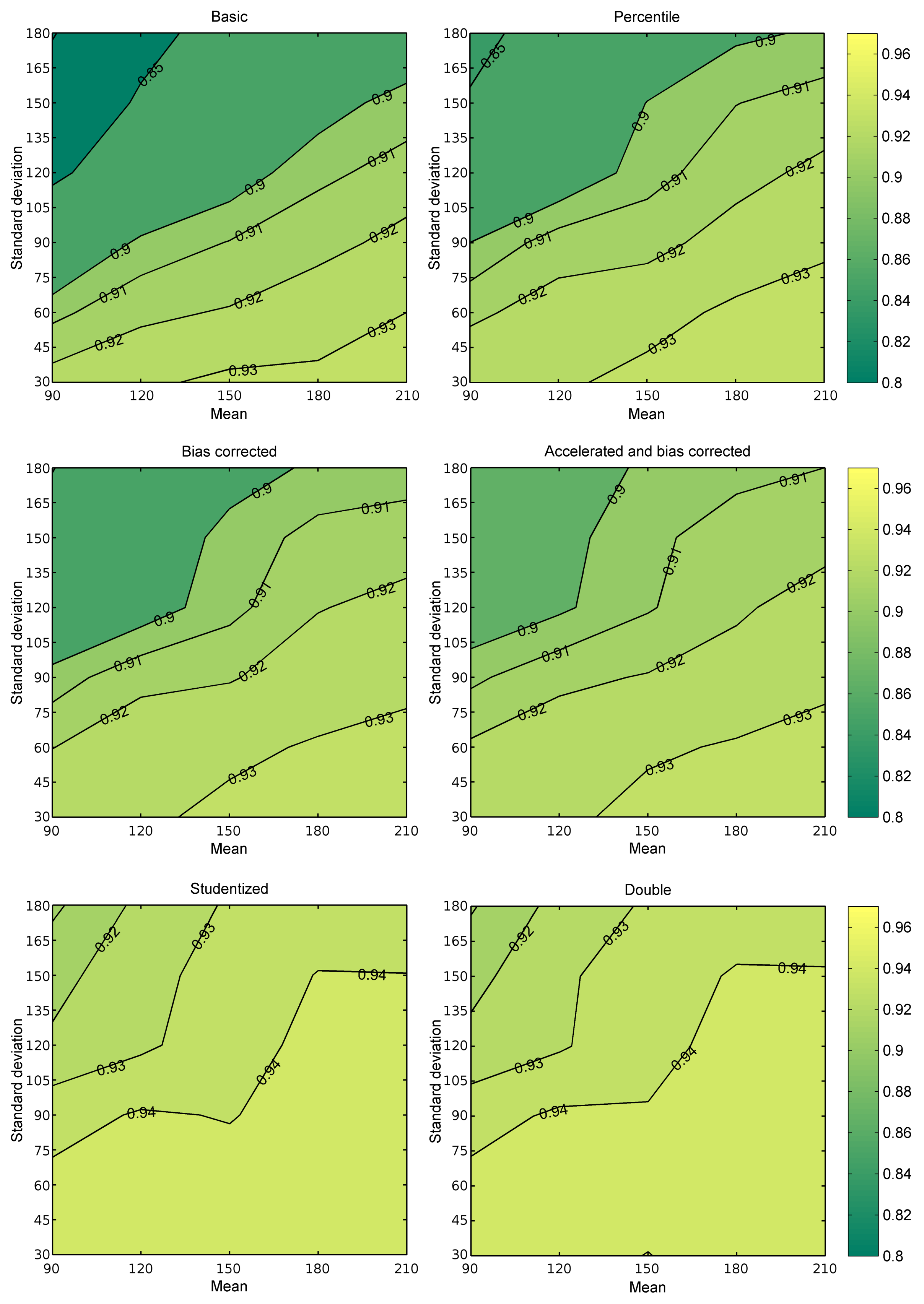
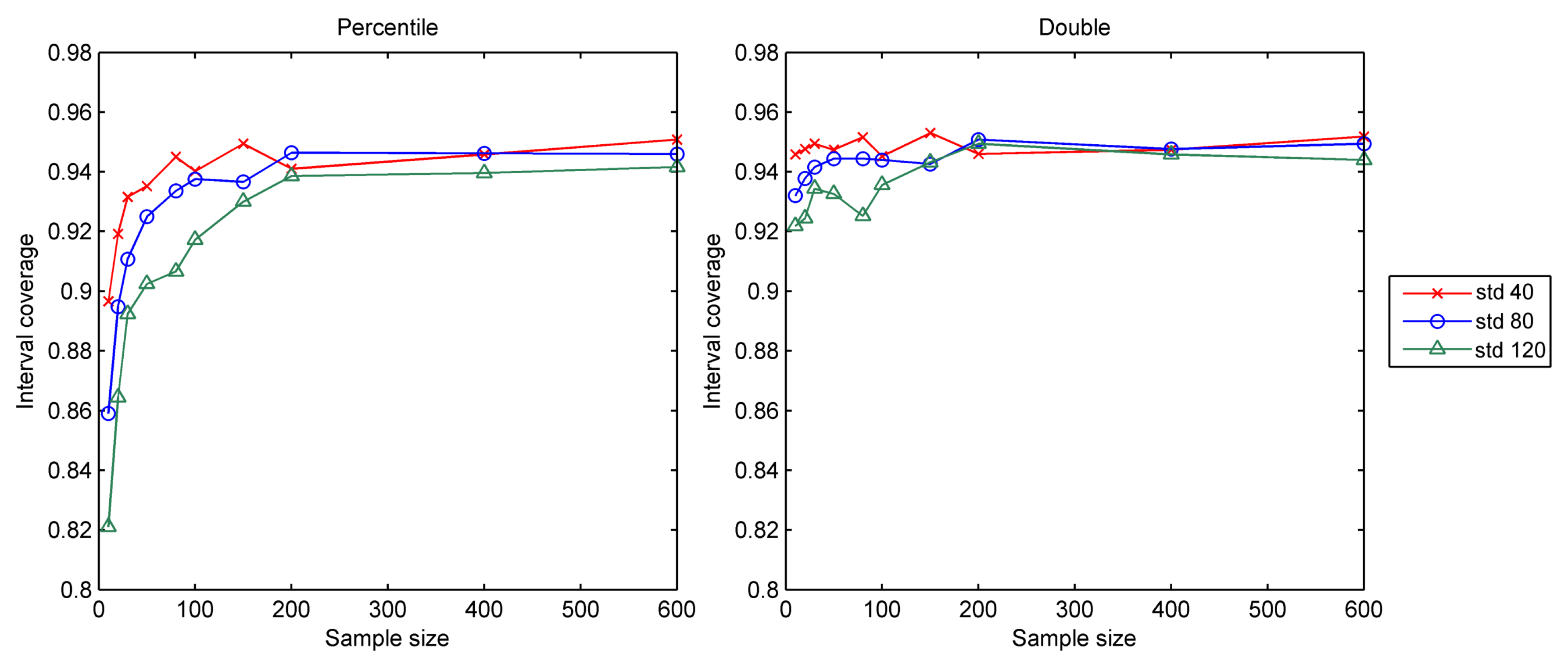
The coverage of intervals obtained using the studentized and double bootstrap methods is less sensitive to the variability of the feature, compared with the basic and percentile methods. For small sample sizes, a confidence level of 93% or more can be obtained if the coefficient of variation does not exceed certain values. For example, if the sample size is ca. 30 elements, the standard deviation of the sample cannot be higher than 22%–33%, 25%–36%, 25%–34%, 23%–33%, 109%–123% and 110%–123% of the sample mean for the basic, percentile, bias-corrected, bias-corrected and accelerated, studentized and double bootstrap methods, respectively.

-

Determining the confidence interval for the expected value of droplet size using bootstrap methods requires knowledge of the exact diameters of individual traces, that is, using image analysis or another measurement method, such as laser droplet size measurement. However, the method presented in this work allows the analysis of surface coverage.

References

1. Cheng, X.; Shuai, C.; Liu, J.; Wang, J.; Liu, Y.; Li, W.; Shuai, J. Modelling environment and poverty factors for sustainable agriculture in the Three Gorges Reservoir of China. Land Degrad. Dev. 2018, 29, 3940–3953. [Google Scholar] [CrossRef]
2. Kiełbasa, B.; Pietrzak, S.; Ulén, B.; Drangert, J.O.; Tonderski, K. Sustainable agriculture: The study on farmers’ perception and practices regarding nutrient management and limiting losses. J. Water Land Dev. 2018, 36, 67–75. [Google Scholar] [CrossRef] [Green Version]
3. Öhlund, E.; Zurek, K.; Hammer, M. Towards sustainable agriculture? The EU framework and local adaptation in Sweden and Poland. Environ. Policy Gov. 2015, 25, 270–287. [Google Scholar] [CrossRef]
4. Piesik, D. Biologiczna walka z chwastami na przykładzie Rumex confertus Willd. Postępy Nauk Rolniczych 2001, 3, 85–98. [Google Scholar]
5. Biziuk, M.; Hupka, J.; Warendecki, W.; Zygmunt, B.; Siłwoiecki, A.; Zelechowska, A.; Dąbrowski, Ł.; Wiergowski, M.; Zaleska, A.; Tyszkiewicz, H. Pestycydy: Występowanie, Oznaczanie i Unieszkodliwianie; Wydawnictwo Naukowo-Techniczne: Warszawa, Poland, 2001. [Google Scholar]
6. Lipa, J.J. Zwalczanie szkodników, chwastów i patogenów. Zesz. Probl. Postęp. Nauk Rol., Rol. Ekol. 1987, 324, 131–155. [Google Scholar]
7. Miłkowski, P.; Woźnica, Z. Zachowanie się kropel opryskowych na powierzchni roślin a skuteczność chwastobójcza Glifosatu. Pr. Kom. Nauk Roln. Kom. Nauk Lesn., Poznan. Tow. Przyj. Nauk 2001, 91, 77–85. [Google Scholar]
8. Sawa, J.; Huyghebaert, B.; Koszel, M. Parametry pracy opryskiwaczy a jakość oprysku. In Proceedings of the 4th Conference: “Racjonalna Technika Ochrony Roślin”, Skierniewice, Poland, 15–16 October 2003; pp. 84–89. [Google Scholar]
9. Miczulski, B. Podstawy Praktycznej Ochrony Roślin; Wydawnictwo Akademii Rolniczej w Lublinie: Lublin, Poland, 1991. [Google Scholar]
10. Rogalski, L.; Konopka, W. Wybrane charakterystyki opryskiwania pszenicy w zależności od wartości dawki cieczy użytkowej. Zesz. Probl. Postęp. Nauk Rol. 2002, 486, 367–373. Available online: http://agro.icm.edu.pl/ agro/element/bwmeta1.element.agro-c9aa0840-51cb-4418-a22e-1e912970f2f1/c/367-373.pdf (accessed on 25 October 2019).
11. Rogalski, L.; Konopka, W. Bilansowanie rozchodu masy oprysku w łanie pszenicy w zależności od rodzaju cieczy użytkowej. Zesz. Probl. Postęp. Nauk Rol. 2002, 486, 375–380. [Google Scholar]
12. Nilars, T.; Taylor, B.; Kappel, D. Wpływ rozpylaczy na jakość i bezpieczeństwo opryskiwania. In Proceedings of the 3rd Conference: “Racjonalna Technika Ochrony Roślin”, Skierniewice, Poland, 16–17 October 2002; pp. 121–134. [Google Scholar]
13. Marshall, J.S.; Palmer, W.M.K. The distribution of raindrops with size. J. Meteorol. 1948, 5, 165–166. [Google Scholar] [CrossRef]
14. Kozu, T.; Nakamura, K. Rainfall parameter estimation from dual-radar measurements combining reflectivity profiles and path-integrated attenuation. J. Atmos. Ocean. Technol. 1991, 8, 259–270. [Google Scholar] [CrossRef] [Green Version]
15. Su, C.L.; Chu, Y.H. Analysis of terminal velocity and VHF backscatter of precipitation particles using Chung-Li VHF radar combined with ground-based disdrometer. Terr. Atmos. Ocean. Sci. 2007, 18, 97–116. [Google Scholar] [CrossRef] [Green Version]
16. Ulbrich, C.W. Natural variations in the analytical form of the raindrop size distribution. J. Appl. Meteorol. 1983, 22, 1764–1775. [Google Scholar] [CrossRef] [Green Version]
17. Maguire, W.B.; Avery, S.K. Retrieval of raindrop size distribution using two Doppler wind profilers: Model sensitivity testing. J. Appl. Meteorol. Climatol. 1994, 33, 1623–1635. [Google Scholar] [CrossRef] [Green Version]
18. Feingold, G.; Levin, Z. Application of the lognormal raindrop distribution to differential reflectivity radar measurement (ZDR). J. Atmos. Ocean. Technol. 1987, 4, 377–382. [Google Scholar] [CrossRef] [Green Version]
19. Meneghini, R.; Rincon, R.; Liao, L. On the use of the lognormal particle size distribution to characterize global rain. In Proceedings of the International Geoscience and Remote Sensing Symposium, Toulouse, France, 21–25 July 2003; pp. 1707–1709. [Google Scholar] [CrossRef] [Green Version]
20. Kuna-Broniowski, M.; Kuna-Broniowska, I. The use of comparators for automatic classification of the splashed rain drops. Electron. J. Pol. Agric. Univ. Agric. Eng. 2001, 4, #08. Available online: http: //www.ejpau.media.pl/volume4/issue2/engineering/art-08.html (accessed on 25 October 2019).
21. Wilks, D.S. Rainfall intensity, the Weibull distribution, and estimation of daily surface runoff. J. Appl. Meteorol. 1989, 28, 52–58. [Google Scholar] [CrossRef] [Green Version]
22. Joss, J.; Waldvogel, A. Raindrop size distribution and sampling size errors. J. Atmos. Sci. 1969, 26, 566–569. [Google Scholar] [CrossRef] [Green Version]
23. Efron, B.; Tibshirani, R.J. Statistical data analysis in the computer age. Science 1991, 253, 390–395. [Google Scholar] [CrossRef] [Green Version]
24. Efron, B.; Tibshirani, R.J. An introduction to the Bootstrap; Chapman & Hall: New York, NY, USA, 1993. [Google Scholar] [CrossRef]
25. Kamińska, J.; Machowczyk, A.; Szewrański, S. The variation of drop size gamma distribution parameters for different natural rainfall intensity, Wydawnictwo ITP. Woda-Środ.-Obsz. Wiej. 2010, 10, 95–102. Available online: http://yadda.icm.edu.pl/baztech/element/bwmeta1.element.baztech-article-BATC-0005-0103 (accessed on 25 October 2019).
26. Hall, P. The Bootstrap and Edgeworth Expansion; Springer: New York, NY, USA, 1992. [Google Scholar] [CrossRef]
27. Pekasiewicz, D. Bootstrapowa weryfikacja hipotez o wartości oczekiwanej populacji o rozkładzie asymetrycznym. Acta Univ. Lodz. Folia Oeconomica 2012, 271, 151–159. Available online: http://cejsh. icm.edu.pl/cejsh/element/bwmeta1.element.hdl_11089_1928/c/Pekasiewicz_151-159.pdf (accessed on 25 October 2019).
28. Zhou, X.; Gao, S. Confidence intervals for the log-normal mean. Stat. Med. 1997, 16, 783–790. [Google Scholar] [CrossRef]
29. Land, C.E. An evaluation of approximate confidence interval estimation methods for lognormal means. Technometrics 1972, 14, 145–158. [Google Scholar] [CrossRef]
30. Angus, J.E. Inferences on the lognormal mean for complete samples. Commun. Stat. Simul. Comput. 1988, 17, 1307–1331. [Google Scholar] [CrossRef]
31. Angus, J.E. Bootstrap one-sided confidence intervals for the lognormal mean. Statistician 1994, 43, 395–401. [Google Scholar] [CrossRef]
32. Krishnamoorthy, K.; Mathew, T.P. Inferences on the means of lognormal distributions using generalized p-values and generalized confidence intervals. J. Stat. Plan. Inference 2003, 115, 103–121. [Google Scholar] [CrossRef]
33. Efron, B. The Jackknife, the Bootstrap, and Other Resampling Plans; Society for Industrial and Applied Mathematics: Philadelphia, PA, USA, 1982. [Google Scholar] [CrossRef]
34. Ozkan, H.E.; Reichard, D.L.; Ackerman, K.D. Effect of orifice wear on spray patterns from fan nozzles. Trans. ASAE 1992, 35, 1091–1096. [Google Scholar] [CrossRef]
35. Efron, B. Better Bootstrap Confidence Intervals. J. Am. Stat. Assoc. 1987, 82, 171–185. [Google Scholar] [CrossRef]
36. McCullough, B.D.; Vinod, H.D. Implementing the Double Bootstrap. Comput. Econ. 1998, 12, 79–95. [Google Scholar] [CrossRef]
37. Maleksaeidi, H.; Karami, E. Social-ecological resilience and sustainable agriculture under water scaricity. Agroecol. Sustain. Food Syst. 2013, 37, 262–290. [Google Scholar] [CrossRef]
38. Tikhonovich, I.A.; Provorov, N.A. Microbiology Is a basis of sustainable agriculture: An opinion. Ann. Appl. Biol. 2011, 159, 155–168. [Google Scholar] [CrossRef]
39. McNeill, D. The contested discourse of sustainable agriculture. Glob. Policy 2019, 10 (Suppl. 1). [Google Scholar] [CrossRef] [Green Version]
40. Domardzki, K.; Rola, H. Efektywność stosowania niższych dawek herbicydów w zbożach. Pamiętnik Puławski Materiały Konferencji 2000, 120, 53–63. [Google Scholar]
41. Głazek, M.; Mrówczyński, M. Łączne stosowanie agrochemikaliów w nowoczesnej technologii produkcji zbóż. Pamiętnik Puławski Materiały Konferencji 1999, 114, 119–126. [Google Scholar]
42. Szymańska, E. Zużycie chemicznych środków ochrony roślin i możliwości jego ograniczenia w zrównoważonym systemie produkcji zbóż. Pamiętnik Puławski Materiały Konferencji 2000, 120, 439–444. [Google Scholar]
43. De Cock, N.; Massinon, M.; Salah, S.O.T.; Lebeau, F. Investigation on optimal spray properties for ground based agricultural applications using deposition and retention models. Biosyst. Eng. 2017, 162, 99–111. [Google Scholar] [CrossRef] [Green Version]
44. Arvidsson, T.; Bergström, L.; Kreuger, J. Spray drift as influenced by meteorological and technical factors. Pest. Manag. Sci 2011, 67, 586–598. [Google Scholar] [CrossRef]
45. Butts, T.R.; Luck, J.D.; Fritz, B.K.; Hofmann, W.C.; Kruger, G.R. Evaluation of spray pattern uniformity using three unique analyses as impacted by nozzle, pressure, and pulse-width modulation duty cycle. Pest. Manag. Sci. 2019, 75, 1875–1886. [Google Scholar] [CrossRef] [Green Version]
46. Parafiniuk, S.; Milanowski, M.; Subr, A.K. The influence of the water quality of the droplet spectrum produced by agricultural nozzles. Agric. Agric. Sci. Procedia 2015, 7, 203–208. [Google Scholar] [CrossRef]
47. Benkwitz, A.; Lütkepohl, H.; Wolters, J. Comparison of bootstrap confidence intervals for impulse responses of German monetary systems. Macroecon. Dyn. 2001, 5, 81–100. Available online: https://www.researchgate.net/publication/23775280_Comparison_of_Bootstrap_Confidence_ Intervals_for_Impulse_Responses_of_German_Monetary_Systems (accessed on 4 December 2019). [CrossRef] [Green Version]
48. Trichakis, I.; Nikolos, I.; Karatzas, G.P. Comparison of bootstrap confidence intervals for an ANN model of a karstic aquifer response. Hydrol. Process. 2011, 25, 2827–2836. [Google Scholar] [CrossRef]
Figure 1. Example scans of droplet stains from: (a) new spray nozzle (b) spray nozzle in longer use.
Sustainability 11 07037 g001
Figure 2. Histograms of the droplet stain diameters from the experiment and fitted lognormal distribution for new and older nozzles.
Sustainability 11 07037 g002
Figure 3. Coverage probabilities of the mean value by confidence intervals constructed by the six types of bootstrap methods ( n = 30 ).
Sustainability 11 07037 g003
Figure 4. Changes in the length of confidence intervals constructed using nonparametric bootstrap methods depending on the sample size; μ x = 160 μ m, σ x = 65 μ m (B—basic, P—percentile, C—bias corrected, A—accelerated, S—studentized, D—double bootstrap).
Sustainability 11 07037 g004
Figure 5. Changes in the lengths of confidence intervals constructed using nonparametric bootstrap methods (percentile and double bootstrap) depending on the sample size and different values of standard deviation; μ x = 160 μ m.
Sustainability 11 07037 g005
Figure 6. Changes in the empirical confidence level of intervals obtained using the nonparametric bootstrap methods depending on the sample size; μ x = 160 μ m, σ x = 65 μ m (B—basic, P—percentile, C—bias corrected, A—accelerated, S—studentized, D—double bootstrap).
Sustainability 11 07037 g006
Figure 7. Changes in the empirical confidence level of intervals constructed using nonparametric bootstrap methods (percentile and double bootstrap) depending on the sample size and different values of standard deviation; μ x = 160 μ m.
Sustainability 11 07037 g007